Optimization by Decoded Quantum Interferometry

We introduce Decoded Quantum Interferometry (DQI), a quantum algorithm for reducing classical optimization problems to classical decoding problems by exploiting structure in the Fourier spectrum of the objective function. DQI reduces sparse max-XORSAT to decoding LDPC codes, which can be achieved using powerful classical algorithms such as Belief Propagation (BP). As an initial benchmark, we compare DQI using belief propagation decoding against classical optimization via simulated annealing. In this setting we present evidence that, for a certain family of max-XORSAT instances, DQI with BP decoding achieves a better approximation ratio on average than simulated annealing, although not better than specialized classical algorithms tailored to those instances. We also analyze a combinatorial optimization problem corresponding to finding polynomials that intersect the maximum number of points. There, DQI efficiently achieves a better approximation ratio than any polynomial-time classical algorithm known to us, thus realizing an apparent exponential quantum speedup. Finally, we show that the problem defined by Yamakawa and Zhandry in order to prove an exponential separation between quantum and classical query complexity is a special case of the optimization problem efficiently solved by DQI.

1 Introduction

Here we address the longstanding open question of whether there exist any optimization problems for which quantum computers can offer exponential speedup. Combinatorial optimization problems have the right characteristics to make them attractive targets for quantum computation, in that they have widespread industrial and scientific applications and the bottleneck for solving them is computational power rather than input/output bandwidth or data quality. More precisely, for many combinatorial optimization problems, the best known algorithms use a number of computational steps that scales exponentially in the number of bits needed to describe the problem instance.

Many combinatorial optimization problems are NP-hard. Therefore, under standard complexity-theoretic assumptions, one does not expect to find polynomial time classical or quantum algorithms that can obtain exactly optimal solutions for worst-case instances. Furthermore, for some combinatorial optimization problems, inapproximability results are known which imply that certain approximations to the optima can also not be found classically or quantumly in polynomial time unless certain widely-believed complexity-theoretic assumptions are false [1]. Nevertheless, there remain many ensembles of combinatorial optimization problems for which the approximations achieved by polynomial-time classical algorithms fall short of complexity-theoretic limits. These gaps present a potential opportunity for quantum computers, namely achieving in polynomial time an approximation that requires exponential time to achieve using known classical algorithms.

These characteristics have drawn substantial attention to quantum algorithms for combinatorial optimization over the last three decades. Two of the main lines of attack on this problem are adiabatic optimization [2] and the Quantum Approximate Optimization Algorithm (QAOA) [3]. These both use Hamiltonians as the point of connection between optimization problems and quantum mechanics. Although fruitful and promising [4, 5, 6, 7, 8], these approaches so far have not yielded a definitive answer to whether quantum computers can achieve exponential speedup for optimization.

Here, we propose a new line of attack on this question, which uses interference patterns, rather than Hamiltonians, as the key quantum principle behind the algorithm. We call this algorithm Decoded Quantum Interferometry (DQI). DQI uses a Quantum Fourier Transform to arrange that amplitudes interfere constructively on symbol strings for which the objective value is large, thereby enhancing the probability of obtaining good solutions upon measurement. Whereas Hamiltonian-based approaches are often regarded as exploiting the local structure of the optimization landscape (e.g. tunneling across barriers [9]), our approach instead exploits sparsity that is routinely present in the Fourier spectrum of the objective functions for combinatorial optimization problems and can also exploit more elaborate structure in the spectrum if present.

Before presenting evidence that DQI can obtain better results than known classical algorithms, we quickly illustrate the essence of the DQI algorithm using max-XORSAT as an example of an optimization problem to which it can be applied. Given $B\in\mathbb{F}_{2}^{m\times n}$ and $\mathbf{v}\in\mathbb{F}_{2}^{m}$ with $m>n$, the max-XORSAT problem is to find $\mathbf{x}\in\mathbb{F}_{2}^{n}$ satisfying as many as possible among the $m$ linear mod-2 equations $B\mathbf{x}=\mathbf{v}$. The objective function $f:\mathbb{F}_{2}^{n}\to\mathbb{Z}$ can be taken as the number of equations satisfied minus the number of equations unsatisfied. This can be expressed as

$$f(\mathbf{x})=\sum_{i=1}^{m}(-1)^{v_{i}+\mathbf{b}_{i}\cdot\mathbf{x}},$$ (1)

where $\mathbf{b}_{i}$ is the $i^{\textrm{th}}$ row of $B$. From this expression one can see that the Hadamard transform of $f$ is extremely sparse: it has $m$ nonzero amplitudes, which are on the strings $\mathbf{b}_{1},\ldots,\mathbf{b}_{m}$. The state $\sum_{\mathbf{x}\in\mathbb{F}_{2}^{n}}f(\mathbf{x})\ket{\mathbf{x}}$ is thus easy to prepare. Simply prepare the superposition $\sum_{i=1}^{m}(-1)^{v_{i}}\ket{\mathbf{b}_{i}}$ and apply the quantum Hadamard transform. (Here, for simplicity, we have omitted normalization factors.) Measuring the state $\sum_{\mathbf{x}\in\mathbb{F}_{2}^{n}}f(\mathbf{x})\ket{\mathbf{x}}$ in the computational basis yields a biased sample, where a string $\mathbf{x}$ is obtained with probability proportional to $f(\mathbf{x})^{2}$, which slightly enhances the likelihood of obtaining strings of large objective value relative to uniformly random sampling.

To obtain stronger enhancement, DQI prepares states of the form

$$\ket{P(f)}=\sum_{\mathbf{x}\in\mathbb{F}_{2}^{n}}P(f(\mathbf{x}))\ket{\mathbf{x}},$$ (2)

where $P$ is an appropriately normalized degree-$\ell$ polynomial. As we show in §5, the Hadamard transform of such a state always takes the form

$$\sum_{k=0}^{\ell}\frac{w_{k}}{\sqrt{\binom{m}{k}}}\sum_{\begin{subarray}{c}\mathbf{y}\in\mathbb{F}_{2}^{m}\\ |\mathbf{y}|=k\end{subarray}}(-1)^{\mathbf{v}\cdot\mathbf{y}}\ket{B^{T}\mathbf{y}},$$ (3)

where $w_{0},\ldots,w_{\ell}$ are coefficients that can be efficiently calculated from the coefficients in $P$ and $|\cdot|$ denotes the Hamming weight, i.e. $\ell_{0}$-norm. The DQI algorithm prepares $\ket{P(f)}$ in three steps. The first step is to prepare the state

$$\sum_{k=0}^{\ell}\frac{w_{k}}{\sqrt{\binom{m}{k}}}\ket{k}\sum_{\begin{subarray}{c}\mathbf{y}\in\mathbb{F}_{2}^{m}\\ |\mathbf{y}|=k\end{subarray}}(-1)^{\mathbf{v}\cdot\mathbf{y}}\ket{\mathbf{y}}\ket{B^{T}\mathbf{y}}.$$ (4)

This is relatively straightforward and can be done in $O(m^{2})$ quantum gates, as discussed in §5. The second step is to uncompute $\ket{k}\ket{\mathbf{y}}$ from the first two registers. The third step is to apply a Hadamard transform to the remaining third register, yielding $\ket{P(f)}$.

The second step, of uncomputation, is not straightforward because $B$ is a nonsquare matrix and thus inferring $\mathbf{y}$ from $B^{T}\mathbf{y}$ is an underdetermined linear algebra problem. However, we also know that $|\mathbf{y}|=k\leq\ell$. We show that the problem of solving this underdetermined linear system with a Hamming weight constraint is equivalent to decoding the classical error correcting code $C^{\perp}=\{\mathbf{d}\in\mathbb{F}_{2}^{m}:B^{T}\mathbf{d}=\mathbf{0}\}$ with up to $\ell$ errors.

Given a string in $\mathbb{F}_{2}^{m}$, the decoding problem is to find its nearest codeword in $C^{\perp}$, as measured by Hamming distance. In general decoding is an NP-hard problem [10]. But it becomes easier if one is promised that the number of errors (i.e. the Hamming distance to the nearest codeword) is not too large. When $B$ is very sparse or has certain kinds of algebraic structure, the decoding problem can be solved by polynomial-time classical algorithms even when $\ell$ is large (e.g. linear in $m$). By solving this decoding problem using a reversible implementation of such a classical decoder one uncomputes the initial two registers. Thus, if the decoding algorithm runs in time $T$ then the total runtime of the quantum algorithm to prepare $\ket{P(f)}$ is $\mathcal{O}(T+m^{2})$.

Approximate solutions to the optimization problem are obtained by measuring $\ket{P(f)}$ in the computational basis. The higher the degree of the polynomial in $\ket{P(f)}$, the greater one can bias the measured bit strings toward solutions with large objective value. However, this requires solving a harder decoding problem, as the number of errors is equal to the degree of $P$. In the next section, we summarize how, by making optimal choice of $P$ and judicious choice of decoder, DQI can be a powerful optimizer for some classes of problems.

2 Summary of Results

Our main results, beyond the introduction of the DQI algorithm, are the following.

• We analyze DQI and characterize the expected number of constraints that will be satisfied, given some conditions on the corresponding code. We describe these results in detail in §6.

• We present two examples of optimization problems where DQI is effective. The first example, which we call Optimal Polynomial Intersection (OPI), is an algebraically structured optimization problem, which includes as special cases some hard polynomial-approximation problems that have been previously studied mainly in the contexts of error correction and cryptanalysis. For OPI, we provide evidence that DQI outperforms all known classical algorithms. We discuss OPI in Section 2.2. Our second example is sparse instances of max-XORSAT. This is a much less structured problem, which may be closer to generic industrial optimization problems. For sparse max-XORSAT, we provide evidence that DQI, using a belief propagation decoder, outperforms simulated annealing, although classical algorithms tailored to this instance can still out-perform DQI. We discuss sparse max-XORSAT further in section 2.3.

Before we get into the results, we formalize the general optimization problem that we apply DQI to, which we call max-LINSAT and define as follows.

Definition 2.1.

Let $\mathbb{F}$ be a finite field. For $i=1,\ldots,m$, let $f_{i}:\mathbb{F}\to\{+1,-1\}$ be arbitrary functions. Given a matrix $B\in\mathbb{F}^{m\times n}$ the max-LINSAT problem is to find $\mathbf{x}\in\mathbb{F}^{n}$ maximizing the objective $f(\mathbf{x})=\sum_{i=1}^{m}f_{i}(\sum_{j=1}^{n}B_{ij}x_{j})$.

In this manuscript, we will assume $m=\mathrm{poly}(n)$, and except where noted otherwise, we will take $\mathbb{F}=\mathbb{F}_{p}$ where $p$ is a prime number whose magnitude is polynomial in $n$. Therefore, $f_{1},\ldots,f_{m}$ can be specified explicitly by their truth tables. We take $f_{i}=+1$ to mean constraint $i$ is satisfied and $f_{i}=-1$ to mean constraint $i$ is unsatisfied. Thus, the objective value $f(\mathbf{x})$ is the number of satisfied constraints minus the number of unsatisfied constraints. Specializing max-LINSAT to $\mathbb{F}_{2}$ yields max-XORSAT. If we additionally promise that each row of the matrix $B$ contains at most $k$ nonzero entries then the resulting problem is max-$k$-XORSAT. The special case of max-$k$-XORSAT with $k=2$ is called MAXCUT. As noted in Section 1, these problems are NP-hard; indeed, even the special case of MAXCUT is NP-hard [11]. Thus, we do not expect either classical or quantum algorithms to find exact solutions in polynomial time. Instead, we focus on finding approximate optima, with the goal of finding better approximations with DQI than can be found with polynomial-time classical algorithms.

2.1 Optimal expected number of satisfied constraints

As we quickly illustrated in Section 1 with the special case of max-XORSAT, DQI reduces the problem of approximating max-LINSAT to the problem of decoding the linear code $C^{\perp}$ over $\mathbb{F}_{p}$ whose parity check matrix is $B^{T}$. That is,

$$C^{\perp}=\{\mathbf{d}\in\mathbb{F}_{p}^{m}:B^{T}\mathbf{d}=\mathbf{0}\}.$$ (5)

This decoding problem is to be solved in superposition, such as by a reversible implementation of any efficient classical decoding algorithm. If $C^{\perp}$ can be efficiently decoded out to $\ell$ errors then, given any appropriately normalized degree-$\ell$ polynomial $P$, DQI can efficiently produce the state

$$\ket{P(f)}=\sum_{\mathbf{x}\in\mathbb{F}_{p}^{n}}P(f(\mathbf{x}))\ket{\mathbf{x}}.$$ (6)

Upon measuring in the computational basis one obtains a given string $\mathbf{x}$ with probability proportional to $P(f(\mathbf{x}))^{2}$. One can choose $P$ to bias this distribution toward strings of large objective value. Larger $\ell$ allows this bias to be stronger, but requires the solution of a harder decoding problem.

More quantitatively, in section 6, we prove the following theorem.

Theorem 2.1.

Given a prime $p$ and $B\in\mathbb{F}_{p}^{m\times n}$, let $f(\mathbf{x})=\sum_{i=1}^{m}f_{i}(\sum_{j=1}^{n}B_{ij}x_{j})$ be a max-LINSAT objective function. Suppose $|f_{i}^{-1}(+1)|=r$ for all $i=1,\ldots,m$ and some $r\in\{1,\dots,p-1\}$. Given a degree-$\ell$ polynomial $P$, let $\langle s\rangle$ be the expected number of satisfied constraints for the symbol string obtained upon measuring the corresponding DQI state $\ket{P(f)}$ in the computational basis. Suppose $2\ell+1<d^{\perp}$ where $d^{\perp}$ is the minimum distance of the code $C^{\perp}=\{\mathbf{d}\in\mathbb{F}_{p}^{m}:B^{T}\mathbf{d}=\mathbf{0}\}$, i.e. the minimum Hamming weight of any nonzero codeword in $C^{\perp}$. In the limit $m\to\infty$, with $\ell/m$ fixed, the optimal choice of degree-$\ell$ polynomial $P$ to maximize $\langle s\rangle$ yields

$$\frac{\langle s\rangle}{m}=\left(\sqrt{\frac{\ell}{m}\left(1-\frac{r}{p}\right)}+\sqrt{\frac{r}{p}\left(1-\frac{\ell}{m}\right)}\right)^{2}$$ (7)

if $\frac{r}{p}\leq 1-\frac{\ell}{m}$ and $\frac{\langle s\rangle}{m}=1$ otherwise.

A plot of (7) for $r/p=1/2$ is given in figure 2.

Theorem 2.1 assumes that $2\ell+1<d^{\perp}$, which is the same as requiring that $C^{\perp}$ can be in principle decoded from up to $\ell$ worst-case errors. Further, if we assume that this decoding can be done efficiently, then the DQI algorithm is also efficient. In our analysis, we show how to relax these assumptions, under other plausible assumptions about the code $C^{\perp}$. In particular, in Theorem 7.1 we prove an analog of theorem 2.1 when $2\ell+1>d^{\perp}$; and in Theorem 8.1 we show that even if there is no efficient decoding algorithm for $\ell$ worst-case errors, an efficient algorithm that succeeds with high probability over random errors can be used in the DQI algorithm to efficiently attain (7) with high probability.

Via theorem 2.1, any result on decoding a class of linear codes, whether rigorous or empirical, implies a corresponding result regarding the performance of DQI for solving a class of combinatorial optimization problems which are dual to these codes. This enables two new lines of attack on the question of quantum advantage for optimization. First, rigorous results on efficient decoding imply as corollaries approximation guarantees for DQI applied to combinatorial optimization problems. Second, this theorem allows incremental experiment-driven development of quantum optimization heuristics, even though quantum hardware is not yet mature enough to run DQI. One can generate instances of an optimization problem, test the empirical performance of a classical decoding algorithm by running it on the corresponding codes, and infer the approximation achieved by DQI via (7). This approximation can then be compared against the empirical performance of classical optimization heuristics run on the same instances. This feedback can be used to drive improvements in decoding algorithms, with the goal of beating the classical optimization heuristics with DQI. Such computational experiments can easily be run on max-LINSAT instances with thousands or even millions of variables.

DQI reduces the problem of satisfying a large number of linear constraints to a problem of correcting a large number of errors in a linear code. Decoding linear codes is also an NP-hard problem in general [10]. So, one must ask whether this reduction is ever advantageous. We next present evidence that it can be. All of the problem instances that we describe and all code used in our computer experiments are available at https://zenodo.org/records/13327871.

2.2 Optimal Polynomial Intersection

The example problem which provides our clearest demonstration of the power of DQI is as follows.

Definition 2.2.

Given integers $n<p$ with $p$ prime, an instance of the Optimal Polynomial Intersection (OPI) problem is as follows. Let $F_{1},\ldots,F_{p-1}$ be subsets of the finite field $\mathbb{F}_{p}$. Find the degree $n-1$ polynomial in $Q\in\mathbb{F}_{p}[y]$ that maximizes $f_{\text{OPI}}(Q)=|\{y\in\{1,\ldots,p-1\}:Q(y)\in F_{y}\}|$, i.e. intersects as many of these subsets as possible.

We note that OPI and special cases of it have been studied in several domains. As we discuss more in §9, OPI is related to the list-recovery problem in the coding theory literature, and to the noisy polynomial reconstruction/interpolation in the cryptography literature [12, 13]; however, as discussed more in §9, the classical algorithms from these literatures do not seem to apply in the parameter regime we consider here. We further note that OPI can be viewed as a generalization of the polynomial approximation problem, studied in [14, 15, 16], in which each set $F_{i}$ is a contiguous range of values in $\mathbb{F}_{p}$. Finally, we note that OPI is related to the problem studied by Yamakawa and Zhandry in [17], again in a very different parameter regime. We discuss this connection more at the end of this section and in Section 3.

Below, we explain how to apply DQI to OPI, and set up a parameter regime for OPI where DQI seems to outperform all classical algorithms known to us. We first observe that OPI is equivalent to a special case of max-LINSAT. Let $q_{0},\ldots,q_{n-1}\in\mathbb{F}_{p}$ be the coefficients in $Q$:

$$Q(y)=\sum_{j=0}^{n-1}q_{j}\,y^{j}.$$ (8)

Recall that a primitive element of a finite field is an element such that taking successive powers of it yields all nonzero elements of the field. Every finite field contains one or more primitive elements. Thus, we can choose $\gamma$ to be any primitive element of $\mathbb{F}_{p}$ and re-express the OPI objective function as

$$f_{\text{OPI}}(Q)=|\{i\in\{0,1,\ldots,p-2\}:Q(\gamma^{i})\in F_{\gamma^{i}}\}|.$$ (9)

Next, let

$$f_{i}(x)=\left\{\begin{array}[]{ll}+1&\textrm{if $x\in F_{\gamma^{i}}$}\\ -1&\textrm{otherwise}\end{array}\right.$$ (10)

for $i=0,\ldots,p-2$ and define the matrix $B$ by

$$B_{ij}=\gamma^{i\times j}\quad i=0,\ldots,p-2\quad\quad j=0,\ldots,n-1.$$ (11)

Then the max-LINSAT cost function is $f(\mathbf{q})=\sum_{i=0}^{p-2}f_{i}(\mathbf{b}_{i}\cdot\mathbf{q})$ where $\mathbf{q}=(q_{0},\ldots,q_{n-1})^{T}\in\mathbb{F}_{p}^{n}$. But $\mathbf{b}_{i}\cdot\mathbf{q}=Q(\gamma^{i})$, so $f(\mathbf{q})=2\cdot f_{\text{OPI}}(Q)-(p-1)$ which means that the max-LINSAT cost function $f$ and the OPI cost function $f_{\text{OPI}}$ are equivalent. Thus we have re-expressed our OPI instance as an equivalent instance of max-LINSAT with $m=p-1$ constraints.

We will apply DQI to the case where

$$|f_{i}^{-1}(+1)|=\lfloor p/2\rfloor\quad\forall i=0,\ldots,p-2.$$ (12)

By (12), in the limit of large $p$ we have $|f_{i}^{-1}(+1)|/p\to 1/2$ and $|f_{i}^{-1}(-1)|/p\to 1/2$ for all $i$. We call functions with this property “balanced.”

Figure 1: A stylized example of the Optimal Polynomial Intersection (OPI) problem. For $i\in\mathbb{F}_{p}$, the orange set above the point $i$ represents $F_{i}$. Both of the polynomials $Q_{1}(x)$ and $Q_{2}(x)$ represent solutions that have a large objective value, as they each agree with all but one set $F_{i}$.

When $B$ has the form (11), then $C^{\perp}=\{\mathbf{d}\in\mathbb{F}_{p}^{m}:B^{T}\mathbf{d}=0\}$ is a Reed-Solomon code with alphabet $\mathbb{F}_{p}$, length $m$, dimension $m-n$, and distance $n+1$. Note that our definitions of $m$ and $n$ are inherited from the parameters of the max-LINSAT instances that we start with and are therefore unfortunately in conflict with the meaning usually assigned to these symbols in a coding theory context.

Maximum likelihood decoding for Reed-Solomon codes can be solved in polynomial time out to half the distance of the code, e.g. using the Berlekamp-Welch algorithm [18]. Consequently, in DQI we can take $\ell=\lfloor\frac{n+1}{2}\rfloor$. For the balanced case $r\to p/2$, (7) simplifies to

$$\frac{\langle s\rangle}{m}=\frac{1}{2}+\sqrt{\frac{\ell}{m}\left(1-\frac{\ell}{m}\right)}$$ (13)

As a concrete example, set $n\simeq m/10$. In this case DQI yields solutions where the fraction of constraints satisfied is $1/2+\sqrt{19}/20\simeq 0.7179$. As discussed in §9, and summarized in table 1, this satisfaction fraction exceeds the fraction achieved by any of the classical polynomial-time algorithms that we consider.

Therefore, these Optimal Polynomial Intersection instances demonstrate the power of DQI. Assuming no polynomial-time classical algorithm for this problem is found that can match this fraction of satisfied constraints, this constitutes an example of an exponential quantum speedup. It is noteworthy that our quantum algorithm is not based on a reduction to an Abelian Hidden Subgroup or Hidden Shift problem. The margin of victory for the approximation fraction (0.7179 vs. 0.55) is also satisfyingly large. Nevertheless, it is also of great interest to investigate whether exponential quantum speedup can be obtained for more generic constraint satisfaction problems, with less underlying structure, as we do in the next section.

Before moving on to unstructured optimization problems, we consider whether the algorithm of Yamakawa and Zhandry [17] may be applied to our OPI problem. As discussed in §9.4, the parameters of our OPI problem are such that solutions satisfying all constraints are statistically likely to exist but these exact optima seem to be computationally intractable to find using known classical algorithms. The quantum algorithm of Yamakawa and Zhandry, when it can be used, produces a solution satisfying all constraints. However, the quantum algorithm of Yamakawa and Zhandry has high requirements on the decodability of $C^{\perp}$. Specifically, for the “balanced case” in which $|f_{i}(+1)|\simeq|f_{i}(-1)|$ for all $i$, the requirement is that $C^{\perp}$ can be decoded out to error rate $1/2$. For our OPI example it is not known how to decode $C^{\perp}$ beyond error rate $1/20$, so the quantum algorithm of Yamakawa and Zhandry is not applicable.

2.3 Random Sparse max-XORSAT

In this section, we consider average-case instances from certain families of bounded degree max-$k$-XORSAT. In a max-$k$-XORSAT instance with degree bounded by $D$, each constraint contains at most $k$ variables and each variable is contained in at most $D$ constraints. In other words, the matrix $B\in\mathbb{F}_{2}^{m\times n}$ defining the instance has at most $k$ nonzero entries in any row and at most $D$ nonzero entries in any column. DQI reduces this to decoding the code $C^{\perp}$ whose parity check matrix is $B^{T}$. Codes with sparse parity check matrices are known as Low Density Parity Check (LDPC) codes. Randomly sampled LDPC codes are known to be correctable from a near-optimal number of random errors (asymptotically as $m$ grows) [19]. Consequently, in the limit of large $m$ they can in principle be decoded up to a number of random errors that nearly saturates the information theoretic limit dictated by the rate of the code. When $k$ and $D$ are very small, information-theoretically optimal decoding for random errors can be closely approached by polynomial-time decoders such as belief propagation [20, 21]. This makes sparse max-XORSAT a promising target for DQI.

In this section we focus on benchmarking DQI with standard belief propagation decoding (DQI+BP) against simulated annealing on max-$k$-XORSAT instances. We choose simulated annealing as our primary classical point of comparison because it is often very effective in practice on sparse constraint satisfaction problems and also because it serves as a representative example of local search heuristics. Local search heuristics are widely used in practice and include greedy algorithms, parallel tempering, TABU search, and many quantum-inspired optimization methods. As discussed in §9.1 these should all be expected to have similar scaling behavior with $D$ on average-case max-$k$-XORSAT with bounded degree. Because of simulated annealing’s simplicity, representativeness, and strong performance on average-case constraint satisfaction problems, beating simulated annealing on some class of instances is a good first test for any new classical or quantum optimization heuristic.

It is well-known that max-XORSAT instances become harder to approximate as the degree of the variables is increased [22, 23]. Via DQI, a max-XORSAT instance of degree $D$ is reduced to a problem of decoding random errors for a code in which each parity check contains at most $D$ variables. As $D$ increases, with $m/n$ held fixed, the distance of the code and hence its performance under information-theoretically optimal decoding are not degraded at all. Thus, as $D$ grows, the fraction of constraints satisfied by DQI with information-theoretically optimal decoding would not degrade. In contrast, classical optimization algorithms based on local search yield satisfaction fractions converging toward $1/2$ in the limit $D\to\infty$ which is no better than random guessing. Thus as $D$ grows with $k/D$ fixed, DQI with information-theoretically optimal decoding will eventually surpass all classical local search heuristics. However, for most ensembles of codes, the number of errors correctable by standard polynomial-time decoders such as belief propagation falls increasingly short of information-theoretic limits as the degree $D$ of the parity checks increases. Thus increasing $D$ generically makes the problem harder both for DQI+BP and for classical optimization heuristics.

Despite this challenge, we are able to find some unstructured families of sparse max-XORSAT instances for which DQI with standard belief propagation decoding finds solutions satisfying a larger fraction of constraints than we are able to find using simulated annealing. We do so by tuning the degree distribution of the instances. For example, in §10, we generate an example max-XORSAT instance from our specified degree distribution, which has $31,216$ variables and $50,000$ constraints, where each constraint contains an average of 53.9731 variables and each variable is contained in an average of 86.451 constraints. We find that DQI, using belief propagation decoding, can find solutions in which the fraction of constraints satisfied is $0.835$, whereas by simulated annealing we are unable to satisfy more than $0.815$.

Furthermore, as shown in table 1, DQI+BP also achieves higher satisfaction fraction than we are able to obtain using any of the general-purpose classical optimization algorithms that we tried. However, unlike our OPI example, we do not put this forth as a potential example of exponential quantum advantage. Rather, we are able to construct a tailored classical algorithm specialized to these instances which finds solutions where the fraction of constraints satisfied is $0.88$, thereby slightly beating DQI+BP.

Optimal Polynomial Intersection Algorithm SAT Fraction DQI + Berlekamp-Welch 0.7179 Truncation Heuristic $0.55+o(1)$ Local Search (e.g. SA) $0.5+o(1)$ Algebraic attacks? None found Random Sparse max-XORSAT Algorithm SAT Fraction Tailored Heuristic 0.880 DQI + Belief Propagation 0.835 Truncation Heuristic 0.812 Simulated Annealing 0.815 Greedy Algorithm 0.666 AdvRand 0.554

Table 1: Here, we compare the fraction of constraints achieved efficiently using DQI against applicable classical algorithms for two optimization problems. On the left, we compare DQI, using the Berlekamp-Welch decoder, against the asymptotic behavior classical algorithms for the OPI problem that we define above. We consider the limit where the number of variables goes to infinity and the number of constraints is ten times the number of variables. On the right, we compare DQI, using standard belief propagation as the decoder, against classical algorithms for a randomly-generated sparse instance with irregular degree-distribution specified in §10. We consider an example instance with $31,216$ variables and $50,000$ constraints. The classical algorithms above as well as the classical algebraic attacks on OPI that we considered are defined and discussed in §9.

3 Relation to Prior Work

DQI is related to a family of quantum reductions that originate with the work of Aharonov, Ta-Shma, and Regev in the early 2000s [24, 25]. In this body of work the core idea is to use the convolution theorem to obtain reductions between nearest lattice vector problems and shortest lattice vector problems. The two members of this family of quantum reductions that bear closest relation to DQI are the recent breakthrough of Yamakawa and Zhandry [17] proving an exponential separation between quantum query complexity and classical query complexity for a problem defined using a random oracle, and the reduction by Debris-Alazard, Remaud, and Tillich [26] of an approximate shortest codeword problem to a bounded distance decoding problem. We discuss each of these in turn.

In [17], Yamakawa and Zhandry define an oracle problem that they prove can be solved using polynomially many quantum queries but requires exponentially many classical queries. Their problem is essentially equivalent to max-LINSAT over an exponentially large finite field $\mathbb{F}_{2^{t}}$, where the functions $f_{1},\ldots,f_{m}$ are defined by random oracles. In §11 we recount the exact definition of the Yamakawa-Zhandry problem and show how DQI can be extended to the Yamakawa-Zhandry problem. In the problem defined by Yamakawa and Zhandry, the truth tables for the constraints are defined by random oracles, and therefore, in the language of theorem 2.1, $r/p=1/2$. Furthermore, the Yamakawa-Zhandry instance is designed such that $C^{\perp}$ can be decoded with exponentially small failure probability if half of the symbols are corrupted by errors. Thus, in the language of 2.1, we can take $\ell/m=1/2$. In this case, if we extrapolate (7) to the Yamakawa-Zhandry regime, one obtains $\langle s\rangle/m=1$, indicating that DQI should find a solution satisfying all constraints. (Extrapolation is required because the Yamakawa-Zhandry example does not satisfy $d^{\perp}<2\ell+1$, although it does satisfy a similar requirement that the decoding problem is solvable almost always with $\ell$ random errors. Confidence in this extrapolation is bolstered by the arguments in §7.) Note that the quantum algorithm given by Yamakawa and Zhandry for finding a solution satisfying all constraints is different than DQI, although similar in spirit.

An important difference between our OPI results and the exponential quantum query complexity speedup of Yamakawa and Zhandry is that the latter depends on $\mathbb{F}_{q}$ being an exponentially large finite field. This allows Yamakawa and Zhandry to obtain an information theoretic exponential classical query-complexity lower bound, thus making their separation rigorous. In contrast, our apparent exponential speedup for OPI uses a finite field of polynomial size, in which case the truth tables are polynomial size and known explicitly. This regime is more relevant to real-world optimization problems. The price we pay is that the classical query complexity in this regime is necessarily polynomial. This means that the information-theoretic argument of [17] establishing an exponential improvement in query complexity does not apply in our setting. Instead, we argue heuristically for an exponential quantum speedup, by comparing to known classical algorithms.

Aside from Yamakawa-Zhandry, other prior work that we are aware of which bears some relation to DQI is a quantum reduction from the approximate shortest codeword problem on a code $C$ to the bounded distance decoding problem on its dual $C^{\perp}$, which is due to Debris-Alazard, Remaud, and Tillich [26]. The approximate nearest codeword problem is closely related to max-XORSAT: the max-XORSAT problem is to find the codeword in $C=\{B\mathbf{x}\,|\,\mathbf{x}\in\mathbb{F}_{2}^{n}\}$ that has smallest Hamming distance from a given bit string $\mathbf{v}$, whereas the shortest codeword problem is to find the codeword in $C\setminus\{\mathbf{0}\}$ with smallest Hamming weight. Roughly speaking, then, the shortest codeword problem is the special case of max-XORSAT where $\mathbf{v}=\mathbf{0}$ except that the trivial solution $\mathbf{0}$ is excluded. Although conceptualized quite differently, the reduction of [26] is similar to the $p=2$ special case of DQI in that it is achieved via a quantum Hadamard transform.

Another interesting connection between DQI and prior work appears in the context of planted inference problems, such as planted $k$XOR, where the task is to recover a secret good assignment planted in an otherwise random $k$XOR instance. It has been recently shown that quantum algorithms can achieve polynomial speedups for planted $k$XOR by efficiently constructing a guiding state that has improved overlap with the planted solution [27]. Curiously, the $\ell$-th order guiding state studied in [27] seems related to the $\ell$-th order DQI state presented here. The key conceptual difference is that, to obtain an assignment that satisfies a large number of constraints, the DQI state in this work is measured in the computational basis, whereas the guiding state in [27] is measured in the eigenbasis of the so-called Kikuchi matrix, and subsequently rounded. It is interesting that for the large values of $\ell$ studied in this work, the (Fourier-transformed) Kikuchi matrix asymptotically approaches a diagonal matrix such that its eigenbasis is close to the computational basis.

Lastly, we would like to highlight [28] in which Chailloux and Tillich introduce a method for decoding superpositions of errors, which can be adapted for the uncomputation step needed in DQI. In this manuscript, for the decoding step of DQI, we use classical decoding algorithms implemented as reversible circuits. However, the quantum state we apply these to consists of a quantum superposition over the possible error strings. When we run a classical decoder in superposition, it treats the different syndromes as if they come from a classical probability distribution. This raises the question: is it possible to exploit the coherence of the superposition over errors? A variant of this question was studied in [28], which they call the quantum decoding problem. They give an algorithm to solve the quantum decoding problem based on a technique called unambiguous state discrimination (USD). Roughly speaking, USD is a coherent quantum rotation which allows us to convert bit-flip error into erasure error. If the resulting erasure error rate is small enough, we can decode perfectly using Gaussian elimination. Interestingly, this is efficient regardless of the sparsity of the code. It is indeed possible to use USD for decoding in DQI. However, we curiously find that the resulting performance of this combination of quantum algorithms on instances of max-LINSAT with uniformly random dense $B$ exactly matches that of the classical truncation heuristic.

4 Discussion

Let us now take stock of what our OPI and max-XORSAT examples tell us about the prospect of achieving exponential speedup on industrially relevant optimization problems using DQI. In real-world optimization problems the truth tables of the constraints are typically known explicitly. This is reflected in standard toy models of real-world optimization such as max-$k$-XORSAT whose variables are over polynomial-size alphabets. The exponential separation of Yamakawa and Zhandry is not informative about this regime as it crucially relies on the fact that exponentially many classical queries would be needed to attain sufficient knowledge of the truth table of the random oracle to solve their problem. Our Optimal Polynomial Intersection example over $\mathbb{F}_{p}$ with polynomial $p$ does provide such evidence, assuming no polynomial time classical attack on this problem is found. Thus it eliminates the requirement of exponentially large alphabet but still relies on algebraic structure.

Using randomly generated instances of max-$k$-XORSAT, we consider the scenario of greatest interest for industrial optimization problems, in which the problem instances neither have exponentially large truth tables nor algebraic structure. We find that in some regime, DQI with belief propagation decoding is able to achieve an approximation to the optimum that we are unable to reach using simulated annealing or any of the other general-purpose classical optimization heuristics that we tried. However, we do not outperform all polynomial-time classical algorithms because we are able to devise an algorithm tailor to those instances that performs better than DQI.

A key direction for future research on DQI is finding additional classes of problems, particularly algebraically unstructured ones, for which DQI achieves a better approximation than any polynomial-time classical algorithm. It is worth noting that any putative example will need to be tested against a wide array of classical algorithms beyond the four considered here (simulated annealing, greedy search, truncation heuristic, and AdvRand). Many of the potentially applicable techniques appear in the literature under headings other than max-XORSAT, such as Ising models, QUBO, PUBO, $p$-spin models, max-SAT, max-CUT, graph coloring, and max-E3-LIN2. Applicable methods include continuous variable relaxations to linear or semidefinite programming problems [29], local methods [30, 31], message passing algorithms [32], LDGM decoders [33], as well as methods related to integer programming and constraint programming [34, 35]. Beyond comparisons to other classical algorithms, it would also be interesting to find a problem that DQI can efficiently solve that is provably hard classically, under standard cryptographic assumptions.

A large space remains to be explored regarding different families of optimization problems, different decoders, and different classical optimization algorithms to compete against. In particular, we believe it will be interesting to study the performance of DQI on algebraically unstructured max-XORSAT where the decoding is done by linear program decoders instead of belief propagation, as linear program decoders can in some cases tolerate higher error rates than belief propagation when in the regime of denser parity check matrices [36, 37, 38, 39, 40, 41, 42], which correspond to harder optimization problems.

Lastly, we note that, in the absence of decoding failures, the probability of obtaining a given bit string using DQI is determined solely by that bit string’s objective value. Most other optimization heuristics, such as simulated annealing, lack this guarantee of fair sampling. As shown in [43], uniform sampling from a set of strings with a given property is a powerful primitive closely linked to approximate counting of strings with that property. In general the approximate counting problem is a more difficult computational problem than the search problem of simply finding an example string with that property. This suggests a direction for future research, namely exploring the power of DQI for approximate counting problems.

5 Decoded Quantum Interferometry

Here we describe Decoded Quantum Interferometry. We start with DQI for max-XORSAT, which is the special case of max-LINSAT with $\mathbb{F}=\mathbb{F}_{2}$. Then we describe DQI with $\mathbb{F}=\mathbb{F}_{p}$ for any prime $p$. In each case, our explanation consists of a discussion of the quantum state we intend to create followed by a description of the quantum algorithm used to create it. The generalization of DQI to extension fields is given in §11.

In this section, we assume throughout that $2\ell+1<d^{\perp}$. In some cases we find that it is possible to decode more than $d^{\perp}/2$ errors with high probability, in which case we can use $\ell$ exceeding this bound. This contributes some technical complications to the description and analysis of the DQI algorithm, which we defer to §7.

5.1 DQI for max-XORSAT

5.1.1 DQI Quantum State for max-XORSAT

Given an objective of the form $f=f_{1}+\ldots+f_{m}$ and a degree-$\ell$ univariate polynomial

$$P(f)=\sum_{k=0}^{\ell}\alpha_{k}f^{k},$$ (14)

we can regard $P(f)$ as a degree-$\ell$ multivariate polynomial in $f_{1},\ldots,f_{m}$. Since $f_{1},\ldots,f_{m}$ are $\pm 1$-valued we have $f_{i}^{2}=1$ for all $i$. Consequently, we can express $P(f)$ as

$$P(f)=\sum_{k=0}^{\ell}u_{k}P^{(k)}(f_{1},\ldots,f_{m}),$$ (15)

where $P^{(k)}(f_{1},\ldots,f_{m})$ is the degree-$k$ elementary symmetric polynomial, i.e. the unweighted sum of all $\binom{m}{k}$ products of $k$ distinct factors from $f_{1},\ldots,f_{m}$.

For simplicity, we will henceforth always assume that the overall normalization of $P$ has been chosen so that the state $\ket{P(f)}=\sum_{\mathbf{x}\in\mathbb{F}_{2}^{n}}P(f(\mathbf{x}))\ket{\mathbf{x}}$ has unit norm. In analogy with equation (15), we will write the DQI state $\ket{P(f)}$ as a linear combination of $\ket{P^{(0)}},\ldots,\ket{P^{(\ell)}}$, where

$$\ket{P^{(k)}}:=\frac{1}{\sqrt{2^{n}\binom{m}{k}}}\sum_{\mathbf{x}\in\mathbb{F}_{2}^{n}}P^{(k)}(f_{1}(\mathbf{b}_{1}\cdot\mathbf{x}),\ldots,f_{m}(\mathbf{b}_{m}\cdot\mathbf{x}))\ket{\mathbf{x}}.$$ (16)

From definition 2.1 and equation (1), we have $f_{i}(\mathbf{b}_{i}\cdot\mathbf{x})=(-1)^{v_{i}}(-1)^{\mathbf{b}_{i}\cdot\mathbf{x}}$, so

$$P^{(k)}(f_{1},\ldots,f_{m}) = \sum_{\begin{subarray}{c}i_{1},\ldots,i_{k}\\ \mathrm{distinct}\end{subarray}}f_{i_{1}}\times\ldots\times f_{i_{k}}$$ (17)

$$= \sum_{\begin{subarray}{c}i_{1},\ldots,i_{k}\\ \mathrm{distinct}\end{subarray}}(-1)^{v_{i_{1}}+\ldots+v_{i_{k}}}(-1)^{(\mathbf{b}_{i_{1}}+\ldots+\mathbf{b}_{i_{k}})\cdot\mathbf{x}}$$ (18)

$$= \sum_{\begin{subarray}{c}\mathbf{y}\in\mathbb{F}_{2}^{m}\\ |\mathbf{y}|=k\end{subarray}}(-1)^{\mathbf{v}\cdot\mathbf{y}}(-1)^{(B^{T}\mathbf{y})\cdot\mathbf{x}},$$ (19)

where $|\mathbf{y}|$ indicates the Hamming weight of $\mathbf{y}$. From this we see that the Hadamard transform of $\ket{P^{(k)}}$ is

$$\ket{\widetilde{P}^{(k)}}:=H^{\otimes n}\ket{P^{(k)}}=\frac{1}{\sqrt{\binom{m}{k}}}\sum_{\begin{subarray}{c}\mathbf{y}\in\mathbb{F}_{2}^{m}\\ |\mathbf{y}|=k\end{subarray}}(-1)^{\mathbf{v}\cdot\mathbf{y}}\ket{B^{T}\mathbf{y}}.$$ (20)

If $|\mathbf{y}|<d^{\perp}/2$, then $B^{T}\mathbf{y}$ are all distinct. Therefore, $\ket{\widetilde{P}^{(0)}},\ldots,\ket{\widetilde{P}^{(\ell)}}$ form an orthonormal set provided $\ell<d^{\perp}/2$, and so do $\ket{P^{(0)}},\ldots,\ket{P^{(\ell)}}$. In this case, the DQI state $\ket{P(f)}=\sum_{\mathbf{x}\in\mathbb{F}_{2}^{n}}P(f(\mathbf{x}))\ket{\mathbf{x}}$ can be expressed as

$$\ket{P(f)}=\sum_{k=0}^{\ell}w_{k}\ket{P^{(k)}},$$ (21)

where

$$w_{k}=u_{k}\sqrt{2^{n}\binom{m}{k}},$$ (22)

and $\langle P(f)|P(f)\rangle=\|\mathbf{w}\|^{2}$ where $\mathbf{w}:=(w_{0},\ldots,w_{\ell})^{T}$.

5.1.2 DQI Algorithm for max-XORSAT

With these facts in hand, we now present the DQI algorithm for max-XORSAT. The algorithm utilizes three quantum registers: a weight register comprising $\lceil\log_{2}\ell\rceil$ qubits, an error register with $m$ qubits, and a syndrome register with $n$ qubits.

As the first step in DQI we initialize the weight register in the state

$$\sum_{k=0}^{\ell}w_{k}\ket{k}.$$ (23)

The choice of $\mathbf{w}\in\mathbb{R}^{\ell+1}$ that maximizes the expected number of satisfied constraints can be obtained by solving for the principal eigenvector of an $(\ell+1)\times(\ell+1)$ matrix, as described in §6. Given $\mathbf{w}$, this state preparation can be done efficiently because it is a state of only $\lceil\log_{2}\ell\rceil$ qubits. One way to do this is to use the method from [44] that prepares an arbitrary superposition over $\ell$ computational basis states using $\widetilde{O}(\ell)$ quantum gates.

Next, conditioned on the value $k$ in the weight register, we prepare the error register into the uniform superposition over all bit strings of Hamming weight $k$

$$\to\sum_{k=0}^{\ell}w_{k}\ket{k}\frac{1}{\sqrt{\binom{m}{k}}}\sum_{\begin{subarray}{c}\mathbf{y}\in\mathbb{F}_{2}^{m}\\ |\mathbf{y}|=k\end{subarray}}\ket{\mathbf{y}}.$$ (24)

Efficient methods for preparing such superpositions using $O(\ell m)$ quantum gates have been devised due to applications in physics, where they are known as Dicke states [45, 46]. Next, we apply the phases $(-1)^{\mathbf{v}\cdot\mathbf{y}}$ by performing a Pauli-$Z_{i}$ on each qubit for which $v_{i}=1$, at the cost of $O(m)$ quantum gates

$$\to\sum_{k=0}^{\ell}w_{k}\ket{k}\frac{1}{\sqrt{\binom{m}{k}}}\sum_{|\mathbf{y}|=k}(-1)^{\mathbf{v}\cdot\mathbf{y}}\ket{\mathbf{y}}.$$ (25)

Then, we reversibly compute $B^{T}\mathbf{y}$ into the syndrome register by standard matrix-vector multiplication over $\mathbb{F}_{2}$ at the cost $O(mn)$ quantum gates

$$\to\sum_{k=0}^{\ell}w_{k}\ket{k}\frac{1}{\sqrt{\binom{m}{k}}}\sum_{|\mathbf{y}|=k}(-1)^{\mathbf{v}\cdot\mathbf{y}}\ket{\mathbf{y}}\ket{B^{T}\mathbf{y}}.$$ (26)

From this, to obtain $\ket{\widetilde{P}^{(k)}}$ we need to use the content $\mathbf{s}=B^{T}\mathbf{y}$ of the syndrome register to reversibly uncompute the contents $k,\mathbf{y}$ of the weight and error registers, in superposition. This is the hardest part. We next discuss how to compute $\mathbf{y}$ from $\mathbf{s}$. By solving this problem we also solve the problem of computing $k$ since $k$ is merely the Hamming weight of $\mathbf{y}$.

Recall that $B\in\mathbb{F}_{2}^{m\times n}$ with $m>n$. Let $\mathbf{s}\in\mathbb{F}_{2}^{n}$ be the content of the syndrome register. Given $\mathbf{s}$ it is easy to find a solution $\mathbf{y}_{0}$ to $\mathbf{s}=B^{T}\mathbf{y}_{0}$, for example by using Gaussian elimination. However, the linear system is underdetermined so in general $\mathbf{y}_{0}$ will not equal $\mathbf{y}$. Rather, $\mathbf{y}$ and $\mathbf{y}_{0}$ will differ by an element of the kernel of $B^{T}$, which we will call $\mathbf{c}$. Thus we have

$$\mathbf{y}_{0} = \mathbf{y}+\mathbf{c}$$ (27)

$$B^{T}\mathbf{c} = 0$$ (28)

$$|\mathbf{y}| = k.$$ (29)

Solving for $\mathbf{y}$ is a classic bounded distance decoding problem where $\mathbf{c}$ is an unknown codeword in $C^{\perp}=\{\mathbf{d}\in\mathbb{F}_{2}^{m}:B^{T}\mathbf{d}=0\}$, $\mathbf{y}_{0}$ is the known corrupted codeword, and $\mathbf{y}$ is the unknown error string, which is promised to have Hamming weight $k$. This has a unique solution provided $k$ is less than half the minimum distance of $C^{\perp}$. When this solution can be found efficiently, we can efficiently uncompute the content of the weight and error registers, which can then be discarded. This leaves

$$\to\sum_{k=0}^{\ell}w_{k}\frac{1}{\sqrt{\binom{m}{k}}}\sum_{|\mathbf{y}|=k}(-1)^{\mathbf{v}\cdot\mathbf{y}}\ket{B^{T}\mathbf{y}}$$ (30)

in the syndrome register which we recognize as

$$=\sum_{k=0}^{\ell}w_{k}\ket{\widetilde{P}^{(k)}}.$$ (31)

By taking the Hadamard transform we then obtain

$$\to\sum_{k=0}^{\ell}w_{k}\ket{P^{(k)}}$$ (32)

which is the desired DQI state $\ket{P(f)}$.

5.2 DQI for General max-LINSAT

5.2.1 DQI Quantum State for General max-LINSAT

Recall that max-LINSAT objective takes the form $f(\mathbf{x})=\sum_{i=1}^{m}f_{i}(\mathbf{b}_{i}\cdot\mathbf{x})$ with $f_{i}:\mathbb{F}_{p}\to\{+1,-1\}$. In order to keep the presentation as simple as possible, we restrict attention to the situation where the preimages $F_{i}:=f_{i}^{-1}(+1)$ for $i=1,\ldots,m$ have the same cardinality $r:=|F_{i}|\in\{1,\ldots,p-1\}$. We will find it convenient to work in terms of $g_{i}$ which we define as $f_{i}$ shifted and rescaled so that its Fourier transform

$$\tilde{g}_{i}(y)=\frac{1}{\sqrt{p}}\sum_{x\in\mathbb{F}_{p}}\omega_{p}^{yx}g_{i}(x)$$ (33)

vanishes at $y=0$ and is normalized, i.e. $\sum_{x\in\mathbb{F}_{p}}|g_{i}(x)|^{2}=\sum_{y\in\mathbb{F}_{p}}|\tilde{g}_{i}(y)|^{2}=1$. (Here and throughout, $\omega_{p}=e^{i2\pi/p}$.) In other words, rather than using $f_{i}$ directly, we will use

$$g_{i}(x):=\frac{f_{i}(x)-\overline{f}}{\varphi}$$ (34)

where $\overline{f}:=\frac{1}{p}\sum_{x\in\mathbb{F}_{p}}f_{i}(x)$ and $\varphi:=\left(\sum_{y\in\mathbb{F}_{p}}|f_{i}(y)-\overline{f}|^{2}\right)^{1/2}$. By (34), the sums

$$f(\mathbf{x}) = f_{1}(\mathbf{b}_{1}\cdot\mathbf{x})+\ldots+f_{m}(\mathbf{b}_{m}\cdot\mathbf{x})$$ (35)

$$g(\mathbf{x}) = g_{1}(\mathbf{b}_{1}\cdot\mathbf{x})+\ldots+g_{m}(\mathbf{b}_{m}\cdot\mathbf{x})$$ (36)

are related according to

$$f(\mathbf{x})=g(\mathbf{x})\varphi+m\overline{f}.$$ (37)

We transform the polynomial $P(f(\mathbf{x}))$ into an equivalent polynomial $Q(g(\mathbf{x}))$ of the same degree by substituting in this relation and absorbing the relevant powers of $\varphi$ and $m\overline{f}$ into the coefficients. That is, $Q(g(\mathbf{x}))=P(f(\mathbf{x}))$. As shown in appendix A, $Q(g(\mathbf{x}))$ can always be expressed as a linear combination of elementary symmetric polynomials. That is,

$$Q(g(\mathbf{x})):=\sum_{k=0}^{\ell}u_{k}P^{(k)}(g_{1}(\mathbf{b}_{1}\cdot\mathbf{x}),\dots,g_{m}(\mathbf{b}_{m}\cdot\mathbf{x})).$$ (38)

As in the case of DQI for max-XORSAT above, we write the DQI state

$$\ket{P(f)}=\sum_{\mathbf{x}\in\mathbb{F}_{p}^{n}}P(f(\mathbf{x}))\ket{\mathbf{x}}=\sum_{\mathbf{x}\in\mathbb{F}_{p}^{n}}Q(g(\mathbf{x}))\ket{\mathbf{x}}=\ket{Q(g)}$$ (39)

as a linear combination of $\ket{P^{(0)}},\ldots,\ket{P^{(\ell)}}$ defined as

$$\ket{P^{(k)}}:=\frac{1}{\sqrt{p^{n-k}\binom{m}{k}}}\sum_{\mathbf{x}\in\mathbb{F}_{p}^{n}}P^{(k)}(g_{1}(\mathbf{b}_{1}\cdot\mathbf{x}),\ldots,g_{m}(\mathbf{b}_{m}\cdot\mathbf{x}))\ket{\mathbf{x}}.$$ (40)

By definition,

$$P^{(k)}(g_{1}(\mathbf{b}_{1}\cdot\mathbf{x}),\ldots,g_{m}(\mathbf{b}_{m}\cdot\mathbf{x}))=\sum_{\begin{subarray}{c}i_{1},\ldots,i_{k}\\ \mathrm{distinct}\end{subarray}}\prod_{i\in\{i_{1},\ldots,i_{k}\}}g_{i}(\mathbf{b}_{i}\cdot\mathbf{x}).$$ (41)

Substituting (33) into (41) yields

$$P^{(k)}(g_{1}(\mathbf{b}_{1}\cdot\mathbf{x}),\ldots,g_{m}(\mathbf{b}_{m}\cdot\mathbf{x})) = \sum_{\begin{subarray}{c}i_{1},\ldots,i_{k}\\ \mathrm{distinct}\end{subarray}}\prod_{i\in\{i_{1},\ldots,i_{k}\}}\left(\frac{1}{\sqrt{p}}\sum_{y_{i}\in\mathbb{F}_{p}}\omega_{p}^{-y_{i}\mathbf{b}_{i}\cdot\mathbf{x}}\ \tilde{g}_{i}(y_{i})\right)$$ (42)

$$= \sum_{\begin{subarray}{c}\mathbf{y}\in\mathbb{F}_{p}^{m}\\ |\mathbf{y}|=k\end{subarray}}\frac{1}{\sqrt{p^{k}}}\ \omega_{p}^{-(B^{T}\mathbf{y})\cdot\mathbf{x}}\ \prod_{\begin{subarray}{c}i=1\\ y_{i}\neq 0\end{subarray}}^{m}\tilde{g}_{i}(y_{i}).$$ (43)

From this we see that the Quantum Fourier Transform of $\ket{P^{(k)}}$ is

$$|\widetilde{P}^{(k)}\rangle:=F^{\otimes n}|P^{(k)}\rangle=\frac{1}{\sqrt{\binom{m}{k}}}\sum_{\begin{subarray}{c}\mathbf{y}\in\mathbb{F}_{p}^{m}\\ |\mathbf{y}|=k\end{subarray}}\left(\prod_{\begin{subarray}{c}i=1\\ y_{i}\neq 0\end{subarray}}^{m}\tilde{g}_{i}(y_{i})\right)|B^{T}\mathbf{y}\rangle$$ (44)

where $F_{ij}=\omega_{p}^{ij}/\sqrt{p}$ with $i,j=0,\dots,p-1$. As in the case of max-XORSAT earlier, if $|\mathbf{y}|<d^{\perp}/2$, then $B^{T}\mathbf{y}$ are all distinct. Therefore, if $\ell<d^{\perp}/2$ then $\ket{\widetilde{P}^{(0)}},\ldots,\ket{\widetilde{P}^{(\ell)}}$ form an orthonormal set and so do $\ket{P^{(0)}},\ldots,\ket{P^{(\ell)}}$. Thus, the DQI state $\ket{P(f)}=\sum_{\mathbf{x}\in\mathbb{F}_{p}^{n}}P(f(\mathbf{x}))\ket{\mathbf{x}}$ can be expressed as

$$\ket{P(f)}=\sum_{k=0}^{\ell}w_{k}\ket{P^{(k)}}$$ (45)

where

$$w_{k}=u_{k}\sqrt{p^{n-k}\binom{m}{k}},$$ (46)

and $\langle P(f)|P(f)\rangle=\|\mathbf{w}\|^{2}$.

5.2.2 DQI Algorithm for General max-LINSAT

DQI for general max-LINSAT employs four quantum registers: a weight register comprising $\lceil\log_{2}\ell\rceil$ qubits, a mask register with $m$ qubits, an error register with $m\lceil\log_{2}p\rceil$ qubits, and a syndrome register with $n\lceil\log_{2}p\rceil$ qubits. We will consider the error and syndrome registers as consisting of $m$ and $n$ subregisters, respectively, where each subregister consists of $\lceil\log_{2}p\rceil$ qubits.

The task of DQI is to produce the state $\ket{Q(g)}$, which by construction is equal to $\ket{P(f)}$. We proceed as follows. First, as in the $p=2$ case, we initialize the weight register in the normalized state

$$\sum_{k=0}^{\ell}w_{k}\ket{k}.$$ (47)

Next, conditioned on the value $k$ in the weight register, we prepare the mask register in the corresponding Dicke state

$$\to\sum_{k=0}^{\ell}w_{k}\ket{k}\frac{1}{\sqrt{\binom{m}{k}}}\sum_{\begin{subarray}{c}\bm{\mu}\in\{0,1\}^{m}\\ |\bm{\mu}|=k\end{subarray}}\ket{\mathbf{\bm{\mu}}}.$$ (48)

Then, we entangle the error register with the mask register. Let $G_{i}$ denote a unitary acting on $\lceil\log_{2}p\rceil$ qubits that sends $\ket{0}$ to

$$\sum_{c_{i}\in\mathbb{F}_{p}}\tilde{g}_{i}(c_{i})\ket{c_{i}},$$ (49)

This may be realized, e.g. using the techniques from [44]. We apply $G_{i}$ to the $i^{\textrm{th}}$ subregister of the error register conditional on the $i^{\textrm{th}}$ qubit in the mask register, which yields

$$\to\sum_{k=0}^{\ell}w_{k}\ket{k}\frac{1}{\sqrt{\binom{m}{k}}}\sum_{|\bm{\mu}|=k}\ket{\bm{\mu}}\prod_{i=1}^{m}G_{i}^{\mu_{i}}\ket{0}^{\otimes m}$$ (50)

$$=\sum_{k=0}^{\ell}w_{k}\ket{k}\frac{1}{\sqrt{\binom{m}{k}}}\sum_{|\bm{\mu}|=k}\ket{\bm{\mu}}\sum_{\mathbf{c}\in\mathbb{F}_{p}^{k}}\tilde{g}_{\mu(1)}(c_{1})\ldots\tilde{g}_{\mu(k)}(c_{k})\ket{\mathbf{c}\hookrightarrow\bm{\mu}}$$ (51)

where $\mu_{i}$ denotes the $i^{\textrm{th}}$ entry of $\bm{\mu}$, $\mu(j)$ denotes the index of the $j^{\textrm{th}}$ nonzero entry of $\bm{\mu}$, and $\mathbf{c}\hookrightarrow\bm{\mu}$ denotes the string in $\mathbb{F}_{p}^{m}$ obtained by substituting the $j^{\textrm{th}}$ entry of $\mathbf{c}$ for the $j^{\textrm{th}}$ nonzero entry in $\bm{\mu}$ and leaving the other entries as zero. (For example $123\hookrightarrow 01011=01023$.)

Next, we reversibly compute $B^{T}(\mathbf{c}\hookrightarrow\bm{\mu})$, into the syndrome register, obtaining the state

$$\to\sum_{k=0}^{\ell}w_{k}\ket{k}\frac{1}{\sqrt{\binom{m}{k}}}\sum_{|\bm{\mu}|=k}\ket{\bm{\mu}}\sum_{\mathbf{c}\in\mathbb{F}_{p}^{k}}\tilde{g}_{\mu(1)}(c_{1})\ldots\tilde{g}_{\mu(k)}(c_{k})\ket{\mathbf{c}\hookrightarrow\bm{\mu}}\ket{B^{T}(\mathbf{c}\hookrightarrow\bm{\mu})}.$$ (52)

By reparametrizing from $f_{1},\ldots,f_{m}$ to $g_{1},\ldots,g_{m}$ we ensured $\tilde{g}_{i}(0)=0$ for all $i$, so in this superposition none of $c_{1},\ldots,c_{k}$ are ever zero. Therefore, the values of $\mathbf{y}=\mathbf{c}\hookrightarrow\bm{\mu}$ appearing in the superposition are exactly

$$\{\mathbf{y}\in\mathbb{F}_{p}^{m}:|\mathbf{y}|=k\}.$$ (53)

The content of the syndrome register is then $B^{T}\mathbf{y}$, and the task of finding $\mathbf{y}$ from $B^{T}\mathbf{y}$ is the bounded distance decoding problem on $C^{\perp}=\{\mathbf{y}\in\mathbb{F}_{p}^{m}:B^{T}\mathbf{y}=\mathbf{0}\}$. The condition that none of the entries of $\mathbf{c}$ are zero ensures that $\mathbf{c}$ and $\bm{\mu}$ are uniquely determined by $\mathbf{c}\hookrightarrow\bm{\mu}$. Moreover, this decomposition is easy to compute. Thus uncomputing the content of the weight, mask, and error registers can be done efficiently whenever the bounded distance decoding problem on $C^{\perp}$ can be solved efficiently out to distance $\ell$.

Uncomputing disentangles the syndrome register from the other registers leaving it in the state

$$\to\sum_{k=0}^{\ell}w_{k}\frac{1}{\sqrt{\binom{m}{k}}}\sum_{|\bm{\mu}|=k}\sum_{\mathbf{c}\in\mathbb{F}_{p}^{k}}\tilde{g}_{\mu(1)}(c_{1})\ldots\tilde{g}_{\mu(k)}(c_{k})\ket{B^{T}(\mathbf{c}\hookrightarrow\bm{\mu})}.$$ (54)

Using the condition $\tilde{g}_{i}(0)=0$, we can rewrite this as

$$=\sum_{k=0}^{\ell}w_{k}\frac{1}{\sqrt{\binom{m}{k}}}\sum_{\begin{subarray}{c}\mathbf{y}\in\mathbb{F}_{p}^{m}\\ |\mathbf{y}|=k\end{subarray}}\left(\prod_{\begin{subarray}{c}i=1\\ y_{i}\neq 0\end{subarray}}^{m}\tilde{g}_{i}(y_{i})\right)\ket{B^{T}\mathbf{y}}.$$ (55)

Comparing (55) with (44) shows that this is equal to

$$=\sum_{k=0}^{\ell}w_{k}\ket{\widetilde{P}^{(k)}}.$$ (56)

Thus, by applying the Quantum Fourier Transform on $\mathbb{F}_{p}^{n}$ to the syndrome register we obtain

$$\to\sum_{k=0}^{\ell}w_{k}\ket{P^{(k)}}.$$ (57)

By the definition of $w_{k}$ this is $\ket{Q(g)}$, which equals $\ket{P(f)}$.

6 Optimal Asymptotic Expected Fraction of Satisfied Constraints

In this section we prove theorem 2.1. Before doing so, we make two remarks. First, we note that the condition $2\ell+1<d^{\perp}$ is equivalent to saying that $\ell$ must be less than half the distance of the code, which is the same condition needed to guarantee that the decoding problem used in the uncomputation step of DQI has a unique solution. This condition is met by our OPI example. It is not met in our irregular max-XORSAT example. In section 7 we show that (7) remains a good approximation even beyond this limit. Second, we note that lemma 6.2 gives an exact expression for the expected number of constraints satisfied by DQI at any finite size and for any choice of polynomial $P$, in terms of a $(\ell+1)\times(\ell+1)$ quadratic form. By numerically evaluating optimum of this quadratic form we find that the finite size behavior converges fairly rapidly to the asymptotic behavior of theorem 2.1, as illustrated in figure 2.

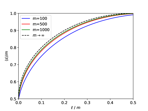
Figure 2: Here we plot the expected fraction $\langle s\rangle/m$ of satisfied constraints, as dictated by lemma 6.2, upon measuring $\ket{P(f)}$ when $P$ is the optimal degree-$\ell$ polynomial. We show the balanced case where $|f_{i}^{-1}(+1)|\simeq p/2$ for all $i$. Accordingly, the dashed black line corresponds to the asymptotic formula (7) with $r/p=1/2$.

6.1 Preliminaries

Recall from §5.2 that the quantum state $|\widetilde{P}(f)\rangle=F^{\otimes n}|P(f)\rangle$ obtained by applying the Quantum Fourier Transform to a DQI state $|P(f)\rangle=\sum_{\mathbf{x}\in\mathbb{F}_{p}^{n}}P(f(\mathbf{x}))|\mathbf{x}\rangle$ is

$$\ket{\widetilde{P}(f)}=\sum_{k=0}^{\ell}\frac{w_{k}}{\sqrt{\binom{m}{k}}}\sum_{\begin{subarray}{c}\mathbf{y}\in\mathbb{F}_{p}^{m}\\ |\mathbf{y}|=k\end{subarray}}\left(\prod_{\begin{subarray}{c}i=1\\ y_{i}\neq 0\end{subarray}}^{m}\tilde{g}_{i}(y_{i})\right)\ket{B^{T}\mathbf{y}}$$ (58)

This can can be written more succinctly as

$$|\widetilde{P}(f)\rangle =\sum_{k=0}^{\ell}\frac{w_{k}}{\sqrt{{m\choose k}}}\sum_{\begin{subarray}{c}\mathbf{y}\in\mathbb{F}_{p}^{m}\\ |\mathbf{y}|=k\end{subarray}}\tilde{g}(\mathbf{y})\ket{B^{T}\mathbf{y}}.$$ (59)

by defining for any $\mathbf{y}\in\mathbb{F}_{p}^{m}$

$$\tilde{g}(\mathbf{y})=\prod_{\begin{subarray}{c}i=1\\ y_{i}\neq 0\end{subarray}}^{m}\tilde{g}_{i}(y_{i}).$$ (60)

Next, we note that

$$\sum_{\begin{subarray}{c}\mathbf{y}\in\mathbb{F}_{p}^{m}\\ |\mathbf{y}|=k\end{subarray}}|\tilde{g}(\mathbf{y})|^{2} =\sum_{\begin{subarray}{c}i_{1},\dots,i_{k}\in\{1,\dots,m\}\\ \text{distinct}\end{subarray}}\left(\sum_{y_{1}\in\mathbb{F}_{p}}|\tilde{g}_{i_{1}}(y_{1})|^{2}\right)\dots\left(\sum_{y_{k}\in\mathbb{F}_{p}}|\tilde{g}_{i_{k}}(y_{k})|^{2}\right)={m\choose k}$$ (61)

where we used the fact that $\tilde{g}_{i}(0)=0$ for all $i$. Lastly, we formally restate the following fact, which we derived in §5.2.

Lemma 6.1.

Let $d^{\perp}$ denote the minimum distance of the code $C^{\perp}=\{\mathbf{d}\in\mathbb{F}_{p}^{m}:B^{T}\mathbf{d}=\mathbf{0}\}$. If $2\ell<d^{\perp}$, then $\langle\widetilde{P}(f)|\widetilde{P}(f)\rangle=\|\mathbf{w}\|^{2}$.

The proof of theorem 2.1 consists of two parts. In the next subsection, we express the expected fraction $\langle s^{(m,\ell)}\rangle/m$ of satisfied constraints as a quadratic form involving a certain tridiagonal matrix. Then, we derive a closed-form asymptotic formula for the maximum eigenvalue of the matrix. We end section 6 by combining the two parts into a proof of theorem 2.1.

6.2 Expected Number of Satisfied Constraints

Lemma 6.2.

Let $f(\mathbf{x})=\sum_{i=1}^{m}f_{i}\left(\sum_{j=1}^{n}B_{ij}x_{j}\right)$ be a max-LINSAT objective function with matrix $B\in\mathbb{F}_{p}^{m\times n}$ for a prime $p$ and positive integers $m$ and $n$ such that $m>n$. Suppose that $|f_{i}^{-1}(+1)|=r$ for some $r\in\{1,\dots,p-1\}$. Let $P$ be a degree-$\ell$ polynomial normalized so that $\langle P(f)|P(f)\rangle=1$ with $P(f)=\sum_{k=0}^{\ell}w_{k}P^{(k)}(f_{1},\ldots,f_{m})/\sqrt{p^{n-k}{m\choose k}}$ its decomposition as a linear combination of elementary symmetric polynomials. Let $\langle s^{(m,\ell)}\rangle$ be the expected number of satisfied constraints for the symbol string obtained upon measuring the DQI state $\ket{P(f)}$ in the computational basis. If $2\ell+1<d^{\perp}$ where $d^{\perp}$ is the minimum distance of the code $C^{\perp}=\{\mathbf{d}\in\mathbb{F}_{p}^{m}:B^{T}\mathbf{d}=\mathbf{0}\}$, then

$$\langle s^{(m,\ell)}\rangle=\frac{mr}{p}+\frac{\sqrt{r(p-r)}}{p}\mathbf{w}^{\dagger}A^{(m,\ell,d)}\mathbf{w}$$ (62)

where $\mathbf{w}=(w_{0},\ldots,w_{\ell})^{T}$ and $A^{(m,\ell,d)}$ is the $(\ell+1)\times(\ell+1)$ symmetric tridiagonal matrix

$$A^{(m,\ell,d)}=\begin{bmatrix}0&a_{1}&\\ a_{1}&d&a_{2}&\\ &a_{2}&2d&\ddots&\\ &&\ddots&&a_{\ell}\\ &&&a_{\ell}&\ell d\end{bmatrix}$$ (63)

with $a_{k}=\sqrt{k(m-k+1)}$ and $d=\frac{p-2r}{\sqrt{r(p-r)}}$.

Proof.

The number of constraints satisfied by $\mathbf{x}\in\mathbb{F}_{p}^{n}$ is

$$s(\mathbf{x})=\sum_{i=1}^{m}\mathbb{1}_{F_{i}}(\mathbf{b}_{i}\cdot\mathbf{x})$$ (64)

where

$$\mathbb{1}_{A}(x)=\begin{cases}1&\text{if}\quad x\in A\\ 0&\text{otherwise}\end{cases}$$ (65)

is the indicator function of the set $A$. For any $v,x\in\mathbb{F}_{p}$, we can write

$$\mathbb{1}_{\{v\}}(x)=\frac{1}{p}\sum_{a\in\mathbb{F}_{p}}\omega_{p}^{a(x-v)}$$ (66)

so

$$\mathbb{1}_{F_{i}}(x)=\sum_{v\in F_{i}}\mathbb{1}_{\{v\}}(x)=\frac{1}{p}\sum_{v\in F_{i}}\sum_{a\in\mathbb{F}_{p}}\omega_{p}^{a(x-v)}.$$ (67)

Substituting into (64), we have

$$s(\mathbf{x})=\frac{1}{p}\sum_{i=1}^{m}\sum_{v\in F_{i}}\sum_{a\in\mathbb{F}_{p}}\omega_{p}^{a(\mathbf{b}_{i}\cdot\mathbf{x}-v)}.$$ (68)

The expected number of constraints satisfied by a symbol string sampled from the output distribution of a DQI state $|P(f)\rangle$ is

$$\langle s^{(m,\ell)}\rangle=\langle P(f)|S_{f}|P(f)\rangle$$ (69)

where $S_{f}=\sum_{\mathbf{x}\in\mathbb{F}_{p}^{n}}s(\mathbf{x})|\mathbf{x}\rangle\langle\mathbf{x}|$. We can express the observable $S_{f}$ in terms of the clock operator $Z=\sum_{b\in\mathbb{F}_{p}}\omega_{p}^{b}|b\rangle\langle b|$ on $\mathbb{C}^{p}$ as

$$S_{f} =\sum_{\mathbf{x}\in\mathbb{F}_{p}^{n}}s(\mathbf{x})|\mathbf{x}\rangle\langle\mathbf{x}|$$ (70)

$$=\frac{1}{p}\sum_{i=1}^{m}\sum_{v\in F_{i}}\sum_{a\in\mathbb{F}_{p}}\sum_{\mathbf{x}\in\mathbb{F}_{p}^{n}}\omega_{p}^{a(\mathbf{b}_{i}\cdot\mathbf{x}-v)}|\mathbf{x}\rangle\langle\mathbf{x}|$$ (71)

$$=\frac{1}{p}\sum_{i=1}^{m}\sum_{v\in F_{i}}\sum_{a\in\mathbb{F}_{p}}\omega_{p}^{-av}\prod_{j=1}^{n}\sum_{x_{j}\in\mathbb{F}_{p}}\omega_{p}^{aB_{ij}x_{j}}|x_{j}\rangle\langle x_{j}|$$ (72)

$$=\frac{1}{p}\sum_{i=1}^{m}\sum_{v\in F_{i}}\sum_{a\in\mathbb{F}_{p}}\omega_{p}^{-av}\prod_{j=1}^{n}Z^{aB_{ij}}.$$ (73)

Next, we apply the Fourier transform $F_{ij}=\omega_{p}^{ij}/\sqrt{p}$ with $i,j=0,\dots,p-1$ to write $\langle s^{(m,\ell)}\rangle$ in terms of the shift operator $X=\sum_{b\in\mathbb{F}_{p}}|b+1\rangle\langle b|$ on $\mathbb{C}^{p}$ as

$$\langle s^{(m,\ell)}\rangle =\frac{1}{p}\sum_{i=1}^{m}\sum_{v\in F_{i}}\sum_{a\in\mathbb{F}_{p}}\omega_{p}^{-av}\langle P(f)|\prod_{j=1}^{n}Z_{j}^{aB_{ij}}|P(f)\rangle$$ (74)

$$=\frac{1}{p}\sum_{i=1}^{m}\sum_{v\in F_{i}}\sum_{a\in\mathbb{F}_{p}}\omega_{p}^{-av}\langle\widetilde{P}(f)|\prod_{j=1}^{n}X_{j}^{-aB_{ij}}|\widetilde{P}(f)\rangle.$$ (75)

where we used $FZF^{\dagger}=X^{-1}$ and $|\widetilde{P}(f)\rangle=F^{\otimes n}|P(f)\rangle$.

Substituting (59) into (75), we get

$$\langle s^{(m,\ell)}\rangle =\frac{1}{p}\sum_{k_{1},k_{2}=0}^{\ell}\frac{w_{k_{1}}^{*}w^{\phantom{*}}_{k_{2}}}{\sqrt{{m\choose k_{1}}{m\choose k_{2}}}}\sum_{\begin{subarray}{c}\mathbf{y}_{1},\mathbf{y}_{2}\in\mathbb{F}_{p}^{m}\\ |\mathbf{y}_{1}|=k_{1}\\ |\mathbf{y}_{2}|=k_{2}\end{subarray}}\tilde{g}^{*}(\mathbf{y}_{1})\tilde{g}(\mathbf{y}_{2})\sum_{i=1}^{m}\sum_{v\in F_{i}}\sum_{a\in\mathbb{F}_{p}}\omega_{p}^{-av}\langle B^{T}\mathbf{y}_{1}|\prod_{j=1}^{n}X_{j}^{-aB_{ij}}|B^{T}\mathbf{y}_{2}\rangle$$ (76)

Let $\mathbf{e}_{1},\dots,\mathbf{e}_{m}\in\mathbb{F}_{p}^{m}$ denote the standard basis of one-hot vectors. Then

$$\prod_{j=1}^{n}X_{j}^{-aB_{ij}}|B^{T}\mathbf{y}_{2}\rangle=|B^{T}\mathbf{y}_{2}-a\mathbf{b}_{i}^{T}\rangle=|B^{T}(\mathbf{y}_{2}-a\mathbf{e}_{i})\rangle$$ (77)

so

$$\langle s^{(m,\ell)}\rangle =\frac{1}{p}\sum_{k_{1},k_{2}=0}^{\ell}\frac{w^{*}_{k_{1}}w^{\phantom{*}}_{k_{2}}}{\sqrt{{m\choose k_{1}}{m\choose k_{2}}}}\sum_{\begin{subarray}{c}\mathbf{y}_{1},\mathbf{y}_{2}\in\mathbb{F}_{p}^{m}\\ |\mathbf{y}_{1}|=k_{1}\\ |\mathbf{y}_{2}|=k_{2}\end{subarray}}\tilde{g}^{*}(\mathbf{y}_{1})\tilde{g}(\mathbf{y}_{2})\sum_{i=1}^{m}\sum_{v\in F_{i}}\sum_{a\in\mathbb{F}_{p}}\omega_{p}^{-av}\langle B^{T}\mathbf{y}_{1}|B^{T}(\mathbf{y}_{2}-a\mathbf{e}_{i})\rangle.$$ (78)

But $|B^{T}\mathbf{y}_{1}\rangle$ and $|B^{T}(\mathbf{y}_{2}-a\mathbf{e}_{i})\rangle$ are computational basis states, so

$$\langle B^{T}\mathbf{y}_{1}|B^{T}(\mathbf{y}_{2}-a\mathbf{e}_{i})\rangle=\begin{cases}1&\text{if}\quad B^{T}\mathbf{y}_{1}=B^{T}(\mathbf{y}_{2}-a\mathbf{e}_{i})\\ 0&\text{otherwise}.\end{cases}$$ (79)

Moreover,

$$B^{T}\mathbf{y}_{1}=B^{T}(\mathbf{y}_{2}-a\mathbf{e}_{i})\iff\mathbf{y}_{1}-\mathbf{y}_{2}+a\mathbf{e}_{i}\in C^{\perp}\iff\mathbf{y}_{1}=\mathbf{y}_{2}-a\mathbf{e}_{i}$$ (80)

where we used the assumption that the smallest Hamming weight of a non-zero symbol string in $C^{\perp}$ is $d^{\perp}>2\ell+1\geq k_{1}+k_{2}+1$.

There are three possibilities to consider: $|\mathbf{y}_{1}|=|\mathbf{y}_{2}|-1$, $|\mathbf{y}_{2}|=|\mathbf{y}_{1}|-1$, and $|\mathbf{y}_{1}|=|\mathbf{y}_{2}|$. We further break up the last case into $\mathbf{y}_{1}\neq\mathbf{y}_{2}$ and $\mathbf{y}_{1}=\mathbf{y}_{2}$. Before simplifying (78), we examine the values of $i\in\{1,\dots,m\}$ and $a\in\mathbb{F}_{p}$ for which $\langle B^{T}\mathbf{y}_{1}|B^{T}(\mathbf{y}_{2}-a\mathbf{e}_{i})\rangle=1$ in each of the four cases. We also compute the value of the product $\tilde{g}^{*}(\mathbf{y}_{1})\tilde{g}(\mathbf{y}_{2})$.

Consider first the case $|\mathbf{y}_{1}|=|\mathbf{y}_{2}|-1$. Here, $a\neq 0$ and $i\in\{1,\dots,m\}$ is the position which is zero in $\mathbf{y}:=\mathbf{y}_{1}$ and $a$ in $\mathbf{y}_{2}$. Therefore, by definition (60)

$$\tilde{g}^{*}(\mathbf{y}_{1})\tilde{g}(\mathbf{y}_{2})=|\tilde{g}(\mathbf{y})|^{2}\tilde{g}_{i}(a).$$ (81)

Next, suppose $|\mathbf{y}_{2}|=|\mathbf{y}_{1}|-1$. Then $a\neq 0$ and $i\in\{1,\dots,m\}$ is the position which is zero in $\mathbf{y}:=\mathbf{y}_{2}$ and $-a$ in $\mathbf{y}_{1}$. Thus,

$$\tilde{g}^{*}(\mathbf{y}_{1})\tilde{g}(\mathbf{y}_{2})=|\tilde{g}(\mathbf{y}_{2})|^{2}\tilde{g}_{i}^{*}(-a)=|\tilde{g}(\mathbf{y})|^{2}\tilde{g}_{i}(a).$$ (82)

Consider next the case $|\mathbf{y}_{1}|=|\mathbf{y}_{2}|$ and $\mathbf{y}_{1}\neq\mathbf{y}_{2}$. Here, $a\neq 0$ and $i\in\{1,\dots,m\}$ is the position which is $z-a$ in $\mathbf{y}_{1}$ and $z$ in $\mathbf{y}_{2}$ for some $z\in\mathbb{F}_{p}\setminus\{0,a\}$. Let $\mathbf{y}\in\mathbb{F}_{p}^{m}$ denote the vector which is zero at position $i$ and agrees with $\mathbf{y}_{1}$, and hence with $\mathbf{y}_{2}$, on all other positions. Then

$$\tilde{g}^{*}(\mathbf{y}_{1})\tilde{g}(\mathbf{y}_{2})=|\tilde{g}(\mathbf{y})|^{2}\tilde{g}_{i}^{*}(z-a)\tilde{g}_{i}(z)=|\tilde{g}(\mathbf{y})|^{2}\tilde{g}_{i}(a-z)\tilde{g}_{i}(z).$$ (83)

Finally, when $\mathbf{y}:=\mathbf{y}_{1}=\mathbf{y}_{2}$, we have

$$\tilde{g}^{*}(\mathbf{y}_{1})\tilde{g}(\mathbf{y}_{2})=|\tilde{g}(\mathbf{y})|^{2}.$$ (84)

In this case, $a=0$ and $i\in\{1,\dots,m\}$.

Putting it all together we can rewrite (78) as

$$\langle s^{(m,\ell)}\rangle =\frac{1}{p}\sum_{k=0}^{\ell-1}\frac{w_{k}^{*}w^{\phantom{*}}_{k+1}}{\sqrt{{m\choose k}{m\choose k+1}}}\sum_{\begin{subarray}{c}\mathbf{y}\in\mathbb{F}_{p}^{m}\\ |\mathbf{y}|=k\end{subarray}}|\tilde{g}(\mathbf{y})|^{2}\sum_{\begin{subarray}{c}i=1\\ y_{i}=0\end{subarray}}^{m}\sum_{v\in F_{i}}\sum_{a\in\mathbb{F}_{p}^{*}}\omega_{p}^{-av}\tilde{g}_{i}(a)$$ (85)

$$+\frac{1}{p}\sum_{k=0}^{\ell-1}\frac{w_{k+1}^{*}w^{\phantom{*}}_{k}}{\sqrt{{m\choose k+1}{m\choose k}}}\sum_{\begin{subarray}{c}\mathbf{y}\in\mathbb{F}_{p}^{m}\\ |\mathbf{y}|=k\end{subarray}}|\tilde{g}(\mathbf{y})|^{2}\sum_{\begin{subarray}{c}i=1\\ y_{i}=0\end{subarray}}^{m}\sum_{v\in F_{i}}\sum_{a\in\mathbb{F}_{p}^{*}}\omega_{p}^{-av}\tilde{g}_{i}(a)$$ (86)

$$+\frac{1}{p}\sum_{k=1}^{\ell}\frac{|w_{k}|^{2}}{{m\choose k}}\sum_{\begin{subarray}{c}\mathbf{y}\in\mathbb{F}_{p}^{m}\\ |\mathbf{y}|=k-1\end{subarray}}|\tilde{g}(\mathbf{y})|^{2}\sum_{\begin{subarray}{c}i=1\\ y_{i}=0\end{subarray}}^{m}\sum_{v\in F_{i}}\sum_{a\in\mathbb{F}_{p}^{*}}\sum_{z\in\mathbb{F}_{p}\setminus\{0,a\}}\omega_{p}^{-av}\tilde{g}_{i}(a-z)\tilde{g}_{i}(z)$$ (87)

$$+\frac{1}{p}\sum_{k=0}^{\ell}\frac{|w_{k}|^{2}}{{m\choose k}}\sum_{\begin{subarray}{c}\mathbf{y}\in\mathbb{F}_{p}^{m}\\ |\mathbf{y}|=k\end{subarray}}|\tilde{g}(\mathbf{y})|^{2}\sum_{i=1}^{m}\sum_{v\in F_{i}}\sum_{a\in\{0\}}\omega_{p}^{-av}.$$ (88)

Remembering that $\tilde{g}_{i}(0)=0$, we recognize the innermost sums in (85) and (86) as the inverse Fourier transform so, for $\mathbf{y}$ with $|\mathbf{y}|=k$, we have

$$\sum_{\begin{subarray}{c}i=1\\ y_{i}=0\end{subarray}}^{m}\sum_{v\in F_{i}}\sum_{a\in\mathbb{F}_{p}^{*}}\omega_{p}^{-av}\tilde{g}_{i}(a)=\sqrt{p}\sum_{\begin{subarray}{c}i=1\\ y_{i}=0\end{subarray}}^{m}\sum_{v\in F_{i}}g_{i}(v)=\sqrt{p}(m-k)r\sqrt{\frac{p-r}{rp}}=(m-k)\sqrt{r(p-r)}.$$ (89)

Similarly, with $\tilde{g}_{i}(0)=0$, we recognize the sums indexed by $a$ and $z$ in (87) as the inverse Fourier transform of the convolution of $\tilde{g}_{i}$ with itself, so

$$\sum_{a\in\mathbb{F}_{p}}\omega_{p}^{-av}\sum_{z\in\mathbb{F}_{p}}\tilde{g}_{i}(a-z)\tilde{g}_{i}(z) =\frac{1}{p}\sum_{a\in\mathbb{F}_{p}}\omega_{p}^{-av}\sum_{z\in\mathbb{F}_{p}}\sum_{x\in\mathbb{F}_{p}}\omega_{p}^{x(a-z)}g_{i}(x)\sum_{y\in\mathbb{F}_{p}}\omega_{p}^{yz}g_{i}(y)$$ (90)

$$=\sum_{a,x,y\in\mathbb{F}_{p}}\omega_{p}^{a(x-v)}g_{i}(x)g_{i}(y)\frac{1}{p}\sum_{z\in\mathbb{F}_{p}}\omega_{p}^{(y-x)z}$$ (91)

$$=\sum_{x\in\mathbb{F}_{p}}g_{i}(x)^{2}\sum_{a\in\mathbb{F}_{p}}\omega_{p}^{a(x-v)}=p\ g_{i}(v)^{2}$$ (92)

and, for $\mathbf{y}$ with $|\mathbf{y}|=k-1$, we have

$$\sum_{\begin{subarray}{c}i=1\\ y_{i}=0\end{subarray}}^{m}\sum_{v\in F_{i}}\sum_{a\in\mathbb{F}_{p}^{*}}\sum_{z\in\mathbb{F}_{p}\setminus\{0,a\}}\omega_{p}^{-av}\tilde{g}_{i}(a-z)\tilde{g}_{i}(z) =\sum_{\begin{subarray}{c}i=1\\ y_{i}=0\end{subarray}}^{m}\sum_{v\in F_{i}}\left(\sum_{a,z\in\mathbb{F}_{p}}\omega_{p}^{-av}\tilde{g}_{i}(a-z)\tilde{g}_{i}(z)-\sum_{z\in\mathbb{F}_{p}}|\tilde{g}_{i}(z)|^{2}\right)$$

$$=\sum_{\begin{subarray}{c}i=1\\ y_{i}=0\end{subarray}}^{m}\sum_{v\in F_{i}}\left(p\ g_{i}(v)^{2}-1\right)$$ (93)

$$=(m-k+1)(p-2r).$$ (94)

Substituting back into (85), (86), and (87), we obtain

$$\langle s^{(m,\ell)}\rangle =\frac{\sqrt{r(p-r)}}{p}\sum_{k=0}^{\ell-1}w^{*}_{k}w^{\phantom{*}}_{k+1}\frac{m-k}{\sqrt{{m\choose k}{m\choose k+1}}}\sum_{\begin{subarray}{c}\mathbf{y}\in\mathbb{F}_{p}^{m}\\ |y|=k\end{subarray}}|\tilde{g}(\mathbf{y})|^{2}$$ (95)

$$+\frac{\sqrt{r(p-r)}}{p}\sum_{k=0}^{\ell-1}w^{*}_{k+1}w^{\phantom{*}}_{k}\frac{m-k}{\sqrt{{m\choose k+1}{m\choose k}}}\sum_{\begin{subarray}{c}\mathbf{y}\in\mathbb{F}_{p}^{m}\\ |y|=k\end{subarray}}|\tilde{g}(\mathbf{y})|^{2}$$ (96)

$$+\frac{p-2r}{p}\sum_{k=1}^{\ell}|w_{k}|^{2}\frac{m-k+1}{{m\choose k}}\sum_{\begin{subarray}{c}\mathbf{y}\in\mathbb{F}_{p}^{m}\\ |y|=k-1\end{subarray}}|\tilde{g}(\mathbf{y})|^{2}$$ (97)

$$+\frac{mr}{p}\sum_{k=0}^{\ell}|w_{k}|^{2}\frac{1}{{m\choose k}}\sum_{\begin{subarray}{c}\mathbf{y}\in\mathbb{F}_{p}^{m}\\ |y|=k\end{subarray}}|\tilde{g}(\mathbf{y})|^{2}$$ (98)

and using equation (61), we get

$$\langle s^{(m,\ell)}\rangle =\frac{\sqrt{r(p-r)}}{p}\sum_{k=0}^{\ell-1}w_{k}^{*}w_{k+1}\sqrt{(k+1)(m-k)}$$ (99)

$$+\frac{\sqrt{r(p-r)}}{p}\sum_{k=0}^{\ell-1}w_{k+1}^{*}w_{k}\sqrt{(k+1)(m-k)}$$ (100)

$$+\frac{p-2r}{p}\sum_{k=0}^{\ell}|w_{k}|^{2}k\,+\,\frac{mr}{p}.$$ (101)

Defining

$$A^{(m,\ell,d)}=\begin{bmatrix}0&a_{1}&\\ a_{1}&d&a_{2}&\\ &a_{2}&2d&\ddots&\\ &&\ddots&&a_{\ell}\\ &&&a_{\ell}&\ell d\end{bmatrix}$$ (102)

where $a_{k}=\sqrt{k(m-k+1)}$ for $k=1,\dots,\ell$ and $d\in\mathbb{R}$, we can write

$$\langle s^{(m,\ell)}\rangle=\frac{mr}{p}+\frac{\sqrt{r(p-r)}}{p}\mathbf{w}^{\dagger}A^{(m,\ell,d)}\mathbf{w}$$ (103)

where $\mathbf{w}=(w_{0},\ldots,w_{\ell})^{T}$ and $d=\frac{p-2r}{\sqrt{r(p-r)}}$. ∎

6.3 Asymptotic Formula for Maximum Eigenvalue of Matrix $A^{(m,\ell,d)}/m$

Lemma 6.3.

Let $\lambda_{\text{max}}^{(m,\ell,d)}$ denote the maximum eigenvalue of the symmetric tridiagonal matrix $A^{(m,\ell,d)}$ defined in (102). If $\ell\leq m/2$ and $d\geq-\frac{m-2\ell}{\sqrt{\ell(m-\ell)}}$, then

$$\lim_{\begin{subarray}{c}m,\ell\to\infty\\ \ell/m=\mu\end{subarray}}\frac{\lambda_{\text{max}}^{(m,\ell,d)}}{m}=\mu d+2\sqrt{\mu(1-\mu)}$$ (104)

where the limit is taken as both $m$ and $\ell$ tend to infinity with the ratio $\mu=\ell/m$ fixed.

Proof.

First, we show that if $\ell\leq m/2$, then

$$\lim_{\begin{subarray}{c}m,\ell\to\infty\\ \ell/m=\mu\end{subarray}}\frac{\lambda_{\text{max}}^{(m,\ell,d)}}{m}\geq\mu d+2\sqrt{\mu(1-\mu)}.$$ (105)

Define vector $v^{(m,\ell)}\in\mathbb{R}^{\ell+1}$ as

$$v_{i}^{(m,\ell)}=\begin{cases}0&\text{for}\quad i=0,1,\dots,\ell-\lceil\sqrt{\ell}\rceil\\ \lceil\sqrt{\ell}\rceil^{-1/2}&\text{for}\quad i=\ell-\lceil\sqrt{\ell}\rceil+1,\dots,\ell.\end{cases}$$ (106)

Then, $\|v^{(m,\ell)}\|_{2}^{2}=\frac{\lceil\sqrt{\ell}\rceil}{\lceil\sqrt{\ell}\rceil}=1$. But

$$\lim_{\begin{subarray}{c}m,\ell\to\infty\\ \ell/m=\mu\end{subarray}}\frac{\lambda_{\text{max}}^{(m,\ell,d)}}{m} \geq\lim_{\begin{subarray}{c}m,\ell\to\infty\\ \ell/m=\mu\end{subarray}}\frac{\left(v^{(m,\ell)}\right)^{T}A^{(m,\ell,d)}v^{(m,\ell)}}{m}$$ (107)

$$=\lim_{\begin{subarray}{c}m,\ell\to\infty\\ \ell/m=\mu\end{subarray}}\left(\frac{1}{m\lceil\sqrt{\ell}\rceil}\sum_{k=\ell-\lceil\sqrt{\ell}\rceil+1}^{\ell}kd\right)+\lim_{\begin{subarray}{c}m,\ell\to\infty\\ \ell/m=\mu\end{subarray}}\left(\frac{1}{m\lceil\sqrt{\ell}\rceil}\sum_{k=\ell-\lceil\sqrt{\ell}\rceil+2}^{\ell}2a_{k}\right).$$ (108)

The second term in (108) is bounded below by

$$\lim_{\begin{subarray}{c}m,\ell\to\infty\\ \ell/m=\mu\end{subarray}}\left(\frac{1}{m\lceil\sqrt{\ell}\rceil}\sum_{k=\ell-\lceil\sqrt{\ell}\rceil+2}^{\ell}2a_{k}\right) \geq\lim_{\begin{subarray}{c}m,\ell\to\infty\\ \ell/m=\mu\end{subarray}}\left(\frac{2a_{\ell-\lceil\sqrt{\ell}\rceil+2}(\lceil\sqrt{\ell}\rceil-1)}{m\lceil\sqrt{\ell}\rceil}\right)$$ (109)

$$=\lim_{\begin{subarray}{c}m,\ell\to\infty\\ \ell/m=\mu\end{subarray}}\left(\frac{2\sqrt{(\ell-\lceil\sqrt{\ell}\rceil+2)(m-\ell+\lceil\sqrt{\ell}\rceil-1)}}{m}\cdot\frac{\lceil\sqrt{\ell}\rceil-1}{\lceil\sqrt{\ell}\rceil}\right)$$

$$=2\sqrt{\mu(1-\mu)}$$ (110)

where we used the fact that $a_{k}$ increases as a function of $k$ for $k\leq m/2$. If $d\geq 0$, then the first term in (108) is bounded below by

$$\lim_{\begin{subarray}{c}m,\ell\to\infty\\ \ell/m=\mu\end{subarray}}\left(\frac{1}{m\lceil\sqrt{\ell}\rceil}\sum_{k=\ell-\lceil\sqrt{\ell}\rceil+1}^{\ell}kd\right) \geq\lim_{\begin{subarray}{c}m,\ell\to\infty\\ \ell/m=\mu\end{subarray}}\quad\frac{\lceil\sqrt{\ell}\rceil\cdot(\ell-\lceil\sqrt{\ell}\rceil+1)\cdot d}{m\lceil\sqrt{\ell}\rceil}=\mu d$$ (111)

and if $d<0$, then it is bounded below by

$$\lim_{\begin{subarray}{c}m,\ell\to\infty\\ \ell/m=\mu\end{subarray}}\left(\frac{1}{m\lceil\sqrt{\ell}\rceil}\sum_{k=\ell-\lceil\sqrt{\ell}\rceil+1}^{\ell}kd\right) \geq\lim_{\begin{subarray}{c}m,\ell\to\infty\\ \ell/m=\mu\end{subarray}}\quad\frac{\lceil\sqrt{\ell}\rceil\cdot\ell\cdot d}{m\lceil\sqrt{\ell}\rceil}=\mu d.$$ (112)

Putting it all together, we get

$$\lim_{\begin{subarray}{c}m,\ell\to\infty\\ \ell/m=\mu\end{subarray}}\frac{\lambda_{\text{max}}^{(m,\ell,d)}}{m}\geq\mu d+2\sqrt{\mu(1-\mu)}.$$ (113)

Next, we establish a matching upper bound on $\lambda_{\text{max}}^{(m,\ell)}$. For $k=0,1,\ldots,\ell$, let $R_{k}^{(m,\ell)}$ denote the sum of the off-diagonal entries in the $k^{\textrm{th}}$ row of $A^{(m,\ell)}$ and set $a_{0}=a_{\ell+1}=0$, so that $R_{k}=a_{k}+a_{k+1}$. By Gershgorin’s circle theorem, for every eigenvalue $\lambda^{(m,\ell)}$ of $A^{(m,\ell)}$, we have

$$\lambda^{(m,\ell,d)} \leq\max_{k\in\{0,\dots,\ell\}}(kd+R_{k})$$ (114)

$$=\max_{k\in\{0,\dots,\ell\}}\left(kd+\sqrt{k(m-k+1)}+\sqrt{(k+1)(m-k)}\right)$$ (115)

$$\leq\max_{k\in\{0,\dots,\ell\}}\left(kd+2\sqrt{(k+1)(m-k)}\right)$$ (116)

$$\leq\max_{k\in\{0,\dots,\ell\}}\left(kd+2\sqrt{k(m-k)}+2\sqrt{m-k}\right)$$ (117)

$$\leq 2\sqrt{m}+\max_{k\in\{0,\dots,\ell\}}\left(kd+2\sqrt{k(m-k)}\right)$$ (118)

$$=2\sqrt{m}+\max_{k\in\{0,\dots,\ell\}}\xi(k)$$ (119)

where we define $\xi(x)=xd+2\sqrt{x(m-x)}$. Note that $\xi^{{}^{\prime\prime}}(x)=-\frac{m^{2}}{2[x(m-x)]^{3/2}}<0$ for all $x\in(0,m)$, so the derivative $\xi^{{}^{\prime}}(x)=d+\frac{m-2x}{\sqrt{x(m-x)}}$ is decreasing in this interval. However, by assumption $d\geq-\frac{m-2\ell}{\sqrt{\ell(m-\ell)}}$, so $\xi^{{}^{\prime}}(x)\geq\xi^{{}^{\prime}}(\ell)\geq 0$ for $x\in(0,\ell]$. Therefore, $\xi(x)$ is increasing on this interval and we have

$$\lambda^{(m,\ell,d)}\leq 2\sqrt{m}+\ell d+2\sqrt{\ell(m-\ell)}.$$ (120)

But then

$$\lim_{\begin{subarray}{c}m,\ell\to\infty\\ \ell/m=\mu\end{subarray}}\frac{\lambda_{\text{max}}^{(m,\ell,d)}}{m} \leq\lim_{\begin{subarray}{c}m,\ell\to\infty\\ \ell/m=\mu\end{subarray}}\frac{2\sqrt{m}+\ell d+2\sqrt{\ell(m-\ell)}}{m}=\mu d+2\sqrt{\mu(1-\mu)}$$ (121)

which establishes the matching upper bound and completes the proof of the lemma. ∎

6.4 Optimal Asymptotic Expected Fraction of Satisfied Constraints

In this subsection we use lemmas 6.2 and 6.3 to prove theorem 2.1.

Proof.

Recall from lemma 6.1 that $\|\mathbf{w}\|_{2}=1$. Therefore, the expected number of satisfied constraints is maximized by choosing $\mathbf{w}$ to be the normalized eigenvector of $A^{(m,\ell,d)}$ corresponding to its maximal eigenvalue. This leads to

$$\frac{\langle s^{(m,\ell)}\rangle_{\mathrm{opt}}}{m}=\rho+\sqrt{\rho(1-\rho)}\frac{\lambda_{\max}^{(m,\ell,d)}}{m}$$ (122)

where $\rho=\frac{r}{p}$ and $d=\frac{p-2r}{\sqrt{r(p-r)}}$. Consider first the case of $\frac{r}{p}\leq 1-\frac{\ell}{m}$. Then $\frac{p-r}{r}\geq\frac{\ell}{m-\ell}$ and

$$d=\frac{p-2r}{\sqrt{r(p-r)}}=\sqrt{\frac{p-r}{r}}-\sqrt{\frac{r}{p-r}}\geq\sqrt{\frac{\ell}{m-\ell}}-\sqrt{\frac{m-\ell}{\ell}}=-\frac{m-2\ell}{\sqrt{\ell(m-\ell)}}.$$ (123)

Moreover, $\ell<(d^{\perp}-1)/2\leq(m-1)/2$. Therefore, lemma 6.3 applies and we have

$$\lim_{\begin{subarray}{c}m,\ell\to\infty\\ \ell/m=\mu\end{subarray}}\frac{\langle s^{(m,\ell)}\rangle_{\mathrm{opt}}}{m} =\rho+\sqrt{\rho(1-\rho)}\lim_{\begin{subarray}{c}m,\ell\to\infty\\ \ell/m=\mu\end{subarray}}\frac{\lambda_{\max}^{(m,\ell,d)}}{m}$$ (124)

$$=\rho+\sqrt{\rho(1-\rho)}\left(\mu d+2\sqrt{\mu(1-\mu)}\right)$$ (125)

$$=\mu+\rho-2\mu\rho+2\sqrt{\mu(1-\mu)\rho(1-\rho)}$$ (126)

$$=\left(\sqrt{\mu(1-\rho)}+\sqrt{\rho(1-\mu)}\right)^{2}$$ (127)

for $\rho\leq 1-\mu$. In particular, if $\rho=1-\mu$, then $\left(\sqrt{\mu(1-\rho)}+\sqrt{\rho(1-\mu)}\right)^{2}=1$. But $\langle s^{(m,\ell)}\rangle_{\mathrm{opt}}$ is an increasing function of $r$ that cannot exceed $1$. Consequently,

$$\lim_{\begin{subarray}{c}m,\ell\to\infty\\ \ell/m=\mu\end{subarray}}\frac{\langle s^{(m,\ell)}\rangle_{\mathrm{opt}}}{m}=1$$ (128)

for $\rho>1-\mu$. Putting it all together, we obtain

$$\lim_{\begin{subarray}{c}m,\ell\to\infty\\ \ell/m=\mu\end{subarray}}\frac{\langle s^{(m,\ell)}\rangle_{\mathrm{opt}}}{m}=\begin{cases}\left(\sqrt{\mu(1-\rho)}+\sqrt{\rho(1-\mu)}\right)^{2}&\text{if}\,\,\rho\leq 1-\mu\\ 1&\text{otherwise}\end{cases}$$ (129)

which completes the proof of theorem 2.1. ∎

7 Removing the Minimum Distance Assumption

So far, in our description and analysis of DQI we have always assumed that $2\ell+1<d^{\perp}$. This condition buys us several advantages. First, it ensures that the states $\ket{\widetilde{P}^{(0)}},\ldots,\ket{\widetilde{P}^{(\ell)}}$, from which we construct $\ket{\widetilde{P}(f)}$, form an orthonormal set which implies that

$$\langle\widetilde{P}(f)|\widetilde{P}(f)\rangle=\mathbf{w}^{\dagger}\mathbf{w}.$$ (130)

Second, it allows us to obtain an exact expression for the expected number of constraints satisfied without needing to know the weight distributions of either the code $C$ or $C^{\perp}$, namely for $p=2$

$$\langle s\rangle=\frac{1}{2}m+\frac{1}{2}\mathbf{w}^{\dagger}A^{(m,\ell,0)}\mathbf{w}$$ (131)

where $A^{(m,\ell,d)}$ is the $(\ell+1)\times(\ell+1)$ matrix defined in (63). These facts in turn allow us to prove theorem 2.1.

For the irregular LDPC code described in §10, we can estimate $d^{\perp}$ using the Gilbert-Varshamov bound. By experimentally testing belief propagation, we find that it is able in practice to correct slightly more than $(d^{\perp}-1)/2$ errors. Under this circumstance, equations (130) and (131) no longer hold exactly. Here we show that, if the code is reasonably well-behaved, then these formulas will hold to a good approximation, and therefore 2.1 yields a good estimate of the performance of DQI. In the remainder of this section we first describe precisely what we mean by the DQI algorithm in the case of $2\ell+1\geq d^{\perp}$. (For simplicity, we consider the case $p=2$.) Secondly, we state the assumption we make regarding the code and present evidence that it holds for the code of §10. Lastly, we use this assumption to prove bounds on $\langle\widetilde{P}(f)|\widetilde{P}(f)\rangle$ and $\langle s\rangle/m$.

As the initial step of DQI, we perform classical preprocessing to choose $\mathbf{w}\in\mathbb{R}^{\ell+1}$, which is equivalent to making a choice of degree-$\ell$ polynomial $P$. In the case $2\ell+1<d^{\perp}$ we can exactly compute the choice of $\mathbf{w}$ that maximizes $\langle s\rangle/m$. Specifically, it is the principal eigenvector of $A^{(m,\ell,d)}$ defined in (63). Once we reach or exceed $2\ell+1=d^{\perp}$ the principal eigenvector of this matrix is not the optimal choice. But we can still use it as our choice of $\mathbf{w}$, and as we will argue below, it remains a good choice.

After choosing $\mathbf{w}$, the next step in the DQI algorithm, as discussed in §5.1.2 is to prepare the state

$$\ket{\widetilde{P}(f)}=\sum_{k=0}^{\ell}w_{k}\ket{k}\frac{1}{\sqrt{{m\choose k}}}\sum_{\begin{subarray}{c}\mathbf{y}\in\mathbb{F}_{2}^{m}\\ |\mathbf{y}|=k\end{subarray}}(-1)^{\mathbf{v}\cdot\mathbf{y}}\ket{\mathbf{y}}\ket{B^{T}\mathbf{y}}.$$ (132)

The following step is to uncompute $\ket{k}$ and $\ket{\mathbf{y}}$. When $2\ell+1\geq d^{\perp}$ this uncomputation will not succeed with $100\%$ certainty. This is because the number of errors $\ell$ is large enough so that, by starting from a codeword in $C^{\perp}$ and then flipping $\ell$ bits, the nearest codeword (in Hamming distance) to the resulting string may be a codeword other than the starting codeword. (This is the same reason that $\ket{\widetilde{P}^{(0)}},\ldots,\ket{\widetilde{P}^{(\ell)}}$ are no longer orthogonal and hence the norm of $\sum_{k=0}^{\ell}w_{k}\ket{\widetilde{P}^{(k)}}$ is no longer exactly equal to $\|\mathbf{w}\|$.)

If the decoder succeeds on a large fraction of the errors that are in superposition, one simply postselects on success of the decoder and obtains a normalized state which is a good approximation to the (unnormalized) ideal state $\sum_{k=0}^{\ell}w_{k}\ket{\widetilde{P}^{(k)}}$. The last steps of DQI are to perform a Hadamard transform and then measure in the computational basis, just as in the case of $2\ell+1<d^{\perp}$.

To bound the discrepancy between the performance of the DQI algorithm outlined above and the ideal behavior described by $\langle s\rangle=\frac{1}{2}m+\frac{1}{2}\mathbf{w}^{\dagger}A^{(m,\ell,0)}\mathbf{w}$ (which converges to (7) in the limit of large $m$), we introduce an assumption on the code $C^{\perp}$. Informally, we assume that most bitstrings with weight less than $\ell$ have no nonzero codewords near them. More precisely, we quantify this using $\zeta$, defined as follows.

Definition 7.1.

Let $\mathcal{E}_{k}=\{\mathbf{y}\in\mathbb{F}_{2}^{m}:|\mathbf{y}|=k\}$ denote the Hamming shell of radius $k$. For all $0\leq k\leq\ell$, when choosing a bit string $\mathbf{y}$ uniformly at random from $\mathcal{E}_{k}$, let $\zeta_{k}$ denote the expected number of nonzero codewords with distance at most $\ell+1$ to $\mathbf{y}$, and let $\zeta=\max_{0\leq k\leq\ell}\zeta_{k}$.

That is, $\zeta$ satisfies the following inequality for all $0\leq k\leq\ell:$

$$\zeta\geq\frac{1}{\binom{m}{k}}\sum_{|\mathbf{y}|=k}\sum_{|\mathbf{y}^{\prime}|\leq\ell+1}\mathbb{1}_{C^{\perp}\backslash\{0\}}(\mathbf{y}+\mathbf{y^{\prime}})=\frac{1}{\binom{m}{k}}\sum_{|\mathbf{y}|=k}\left|\{\mathbf{z}\in C^{\perp}\backslash\{0\}:|\mathbf{y}-\mathbf{z}|\leq\ell+1\}\right|.$$ (133)

With this definition, the performance of DQI is formalized by theorem 7.1. Our assumption is that $\zeta\ll 1$, as specified in conjecture 7.1, in which case theorem 7.1 converges back to the ideal behavior described in (7) for the case $2\ell+1<d^{\perp}$. Note that if $2\ell+1<d^{\perp}$, $\zeta$ equals zero.

Theorem 7.1.

For fixed $B\in\mathbb{F}_{2}^{m\times n}$ and $\mathbf{v}\in\mathbb{F}_{2}^{m}$ chosen uniformly at random, let $f$ be the objective function $f(\mathbf{x})=\sum_{i=1}^{m}(-1)^{v_{i}+\mathbf{b}_{i}\cdot\mathbf{x}}$. Let $P$ be any degree-$\ell$ polynomial and let $P(f)=\sum_{k=0}^{\ell}w_{k}P^{(k)}\left(f_{1},\ldots,f_{m}\right)/\sqrt{2^{n}\binom{m}{k}}$ be the decomposition of $P(f)$ as a linear combination of elementary symmetric polynomials. Let $\langle f\rangle$ be the expected objective value for the symbol string obtained upon measuring the DQI state $|P(f)\rangle$ in the computational basis. Let $\zeta\geq 0$ be chosen so that equation (133) holds for the code $C^{\perp}$. If $\ell\leq\frac{m}{4}$, then in expectation over the uniform choice of $\mathbf{v}$,

$$\mathbb{E}_{\mathbf{v}}\langle f\rangle\geq\frac{\mathbf{w}^{\dagger}A^{(m,\ell,0)}\mathbf{w}}{(1+4\zeta)\mathbf{w}^{\dagger}\mathbf{w}},$$ (134)

where $A^{(m,\ell,0)}$ is the tridiagonal matrix defined in equation (63). Moreover, for any (potentially worst case) $\mathbf{v}$,

$$\langle f\rangle\geq\frac{\mathbf{w}^{\dagger}A^{(m,\ell,0)}\mathbf{w}-\mathbf{w}^{\dagger}\mathbf{w}\left(4\zeta m\right)}{\left(1+4\zeta\right)\mathbf{w}^{\dagger}\mathbf{w}}.$$ (135)

If one chooses $\mathbf{w}$ to be the principal eigenvector of $A^{(m,\ell,0)}$ then (134) and (135) yield the following results in the limit of large $\ell$ and $m$ with the ratio $\mu=\ell/m$ fixed

$$\lim_{\begin{subarray}{c}m\to\infty\\ \ell/m=\mu\end{subarray}}\frac{\mathbb{E}_{\mathbf{v}}\langle f\rangle}{m}\geq\frac{2\sqrt{\frac{\ell}{m}\left(1-\frac{\ell}{m}\right)}}{1+4\zeta},$$ (136)

$$\lim_{\begin{subarray}{c}m\to\infty\\ \ell/m=\mu\end{subarray}}\frac{\langle f\rangle}{m}\geq\frac{2\sqrt{\frac{\ell}{m}\left(1-\frac{\ell}{m}\right)}-4\zeta}{1+4\zeta}.$$ (137)

Remark 7.1.

For comparison, theorem 2.1 implies that if $2\ell+1<d^{\perp}$, then

$$\lim_{\begin{subarray}{c}m\to\infty\\ \ell/m=\mu\end{subarray}}\frac{\langle f\rangle}{m}=2\sqrt{\frac{\ell}{m}\left(1-\frac{\ell}{m}\right)}$$ (138)

indicating that the bounds in (136) and (137) become tight as $\zeta\to 0$.

Conjecture 7.1.

For the irregular LDPC code described in §10, the quantity $\zeta$ as defined in definition 7.1 is at most $10^{-4}$.

In Appendix D, we outline several heuristic motivations for this conjecture. Indeed, as discussed in detail in the appendix, we expect $\zeta$ to be much smaller in practice, at most $2^{-500}$.

Corollary 7.1.

For the family of irregular LDPC codes described in §10, conjecture 7.1 together with theorem 7.1 implies that DQI asymptotically achieves an approximation ratio $\langle s\rangle/m$ of at least 0.8346 for any $\mathbf{v}\in\mathbb{F}_{2}^{m}$.

Proof.

Use equation (137) with $\ell=6,437,m=50,000,\zeta=10^{-4}$. ∎

7.1 General Expressions for the Expected Number of Satisfied Constraints

To prove theorem 7.1, we first derive generalizations of lemmas 6.1 and 6.2 for arbitrary code distances. Recall the definition of the (Fourier-transformed) DQI state associated with a degree-$\ell$ multivariate polynomial $P(f)$:

$$|\widetilde{P}(f)\rangle=\sum_{k=0}^{\ell}\frac{w_{k}}{\sqrt{{m\choose k}}}\sum_{\begin{subarray}{c}\mathbf{y}\in\mathbb{F}_{2}^{m}\\ |\mathbf{y}|=k\end{subarray}}(-1)^{\mathbf{v}\cdot\mathbf{y}}\ket{B^{T}\mathbf{y}}.$$ (139)

If $d^{\perp}>2\ell$ then the $B^{T}\mathbf{y}$ are all distinct and the norm of $|\widetilde{P}(f)\rangle$ is the norm of $\mathbf{w}$, as shown in lemma 6.1. More generally, we have the following lemma.

Lemma 7.1.

The squared norm of $|\widetilde{P}(f)\rangle$ is

$$\langle\widetilde{P}(f)|\widetilde{P}(f)\rangle=\mathbf{w}^{\dagger}M^{(m,\ell)}\mathbf{w},$$ (140)

where $M^{(m,\ell)}$ is the $(\ell+1)\times(\ell+1)$ symmetric matrix defined by

$$M_{k,k^{\prime}}^{(m,\ell)}=\frac{1}{\sqrt{\binom{m}{k}\binom{m}{k^{\prime}}}}\sum_{\begin{subarray}{c}\mathbf{y}\in\mathbb{F}_{2}^{m}\\ |\mathbf{y}|=k\end{subarray}}\sum_{\begin{subarray}{c}\mathbf{y}^{\prime}\in\mathbb{F}_{2}^{m}\\ |\mathbf{y}^{\prime}|=k^{\prime}\end{subarray}}(-1)^{(\mathbf{y}+\mathbf{y}^{\prime})\cdot\mathbf{v}}\delta_{B^{T}\mathbf{y},B^{T}\mathbf{y}^{\prime}},$$ (141)

for $0\leq k,k^{\prime}\leq\ell$.

Proof.

This is immediate from (139) and the fact that the $\ket{B^{T}\mathbf{y}}$ are computational basis states. ∎

Note that if $d^{\perp}>2\ell$, then $M^{(m,\ell)}_{k,k^{\prime}}=\delta_{k,k^{\prime}}$, in agreement with lemma 6.1.

Lemma 7.2.

For $B\in\mathbb{F}_{2}^{m\times n}$ and $\mathbf{v}\in\mathbb{F}_{2}^{m}$, let $f$ be the objective function $f(\mathbf{x})=\sum_{i=1}^{m}(-1)^{v_{i}+\mathbf{b}_{i}\cdot\mathbf{x}}$. Let $P$ be any degree-$\ell$ polynomial and let $P(f)=\sum_{k=0}^{\ell}w_{k}P^{(k)}\left(f_{1},\ldots,f_{m}\right)/\sqrt{2^{n}\binom{m}{k}}$ be the decomposition of $P(f)$ as a linear combination of elementary symmetric polynomials. Let $\langle f\rangle$ be the expected objective value for the symbol string obtained upon measuring the DQI state $|P(f)\rangle$ in the computational basis. If the weights $w_{k}$ are such that $|P(f)\rangle$ is normalized, then

$$\langle f\rangle=\mathbf{w}^{\dagger}\bar{A}^{(m,\ell)}\mathbf{w}$$ (142)

where $\bar{A}^{(m,\ell)}$ is the $(\ell+1)\times(\ell+1)$ symmetric matrix defined by

$$\bar{A}^{(m,\ell)}_{k,k^{\prime}}=\frac{1}{\sqrt{\binom{m}{k}\binom{m}{k^{\prime}}}}\sum_{i=1}^{m}\sum_{(\mathbf{y},\mathbf{y^{\prime}})\in S^{(i)}_{k,k^{\prime}}}(-1)^{v_{i}+\mathbf{v}\cdot(\mathbf{y}+\mathbf{y}^{\prime})}$$ (143)

for $0\leq k,k^{\prime}\leq\ell$, and

$$S^{(i)}_{k,k^{\prime}}=\{(\mathbf{y},\mathbf{y}^{\prime})\in\mathbb{F}_{2}^{m}\times\mathbb{F}_{2}^{m}:|\mathbf{y}|=k,|\mathbf{y}^{\prime}|=k^{\prime},B^{T}(\mathbf{y}+\mathbf{y}^{\prime}+\mathbf{e}_{i})=\mathbf{0}\}.$$ (144)

for one-hot vectors $\mathbf{e}_{1},\ldots,\mathbf{e}_{m}$ in $\mathbb{F}_{2}^{m}$.

Proof.

The expected value of $f(\mathbf{x})$ in state $\ket{P(f)}$ is

$$\langle f\rangle=\bra{P(f)}H_{f}\ket{P(f)},$$ (145)

where

$$H_{f}=\sum_{i=1}^{m}(-1)^{v_{i}}\prod_{j:B_{ij}=1}Z_{j}$$ (146)

and $Z_{j}$ denotes the Pauli $Z$ operator acting on the $j^{\textrm{th}}$ qubit. Recalling that conjugation by Hadamard interchanges Pauli $X$ with $Z$, so we have

$$\langle f\rangle = \sum_{i=1}^{m}(-1)^{v_{i}}\bra{P(f)}\prod_{j:B_{ij}=1}Z_{j}\ket{P(f)}$$ (147)

$$= \sum_{i=1}^{m}(-1)^{v_{i}}\bra{\widetilde{P}(f)}\prod_{j:B_{ij}=1}X_{j}\ket{\widetilde{P}(f)}$$ (148)

$$= \sum_{k,k^{\prime}=0}^{\ell}\frac{w_{k}w_{k^{\prime}}}{\sqrt{\binom{m}{k}\binom{m}{k^{\prime}}}}\sum_{|\mathbf{y}|=k}\sum_{|\mathbf{y}^{\prime}|=k^{\prime}}(-1)^{\mathbf{v}\cdot(\mathbf{y}+\mathbf{y}^{\prime})}\sum_{i=1}^{m}(-1)^{v_{i}}\bra{B^{T}\mathbf{y}}\prod_{j:B_{ij}=1}X_{j}\ket{B^{T}\mathbf{y}^{\prime}},$$ (149)

where in the last line we have plugged in the definition of $\ket{\widetilde{P}(f)}$. We can rewrite this quadratic form as

$$\langle f\rangle=\sum_{k,k^{\prime}=0}^{\ell}w_{k}\ w_{k^{\prime}}\ \bar{A}^{(m,\ell)}_{k,k^{\prime}},$$ (150)

where

$$\bar{A}^{(m,\ell)}_{k,k^{\prime}}=\frac{1}{\sqrt{\binom{m}{k}\binom{m}{k^{\prime}}}}\sum_{|\mathbf{y}|=k}\sum_{|\mathbf{y}^{\prime}|=k^{\prime}}(-1)^{\mathbf{v}\cdot(\mathbf{y}+\mathbf{y}^{\prime})}\sum_{i=1}^{m}(-1)^{v_{i}}\bra{B^{T}\mathbf{y}}\prod_{j:B_{ij}=1}X_{j}\ket{B^{T}\mathbf{y}^{\prime}}.$$ (151)

For the one-hot vectors $\mathbf{e}_{1},\ldots,\mathbf{e}_{m}\in\mathbb{F}_{2}^{m}$ we have

$$\prod_{j:B_{ij}=1}X_{j}\ket{B^{T}\mathbf{y}^{\prime}}=\ket{B^{T}(\mathbf{y}^{\prime}+\mathbf{e}_{i})}.$$ (152)

Substituting this into (149) yields

$$\bar{A}^{(m,\ell)}_{k,k^{\prime}}=\frac{1}{\sqrt{\binom{m}{k}\binom{m}{k^{\prime}}}}\sum_{|\mathbf{y}|=k}\sum_{|\mathbf{y}^{\prime}|=k^{\prime}}(-1)^{\mathbf{v}\cdot(\mathbf{y}+\mathbf{y}^{\prime})}\sum_{i=1}^{m}(-1)^{v_{i}}\langle B^{T}\mathbf{y}|B^{T}(\mathbf{y}^{\prime}+\mathbf{e}_{i})\rangle.$$ (153)

We next note that $\langle B^{T}\mathbf{y}|B^{T}(\mathbf{y}^{\prime}+\mathbf{e}_{i})\rangle$ equals one when $B^{T}\mathbf{y}=B^{T}(\mathbf{y}^{\prime}+\mathbf{e}_{i})$ and zero otherwise. The condition $B^{T}\mathbf{y}=B^{T}(\mathbf{y}^{\prime}+\mathbf{e}_{i})$ is equivalent to $B^{T}(\mathbf{y}+\mathbf{y}^{\prime}+\mathbf{e}_{i})=\mathbf{0}$. Hence,

$$\bar{A}^{(m,\ell)}_{k,k^{\prime}}=\frac{1}{\sqrt{\binom{m}{k}\binom{m}{k^{\prime}}}}\sum_{i=1}^{m}\sum_{(\mathbf{y},\mathbf{y^{\prime}})\in S^{(i)}_{k,k^{\prime}}}(-1)^{v_{i}+\mathbf{v}\cdot(\mathbf{y}+\mathbf{y}^{\prime})}$$ (154)

where

$$S^{(i)}_{k,k^{\prime}}=\{(\mathbf{y},\mathbf{y}^{\prime})\in\mathbb{F}_{2}^{m}\times\mathbb{F}_{2}^{m}:|\mathbf{y}|=k,|\mathbf{y}^{\prime}|=k^{\prime},B^{T}(\mathbf{y}+\mathbf{y}^{\prime}+\mathbf{e}_{i})=\mathbf{0}\}.$$ (155)

∎

Note once again that if $d^{\perp}>2\ell+1$ then $\bar{A}^{(m,\ell)}$ simplifies to $A^{(m,\ell,0)}$ defined in (63). It is also easy to verify that $\bar{A}^{(m,\ell)}$ can be rewritten in terms of $M$ as

$$\bar{A}^{(m,\ell)}_{k,k^{\prime}}=\sqrt{k^{\prime}(m-k^{\prime}+1)}M^{(m,\ell)}_{k,k^{\prime}-1}+\sqrt{(k^{\prime}+1)(m-k^{\prime})}M^{(m,\ell)}_{k,k^{\prime}+1},$$ (156)

where we define $M^{(m,\ell)}_{k,k^{\prime}}$ according to formula (141), even if $k$ or $k^{\prime}$ exceed $\ell+1$.

7.2 Proof of Theorem 7.1

To prove theorem 7.1, we combine lemmas 7.1 and 7.2. They show that for an arbitrary weight vector $\mathbf{w}$, the expected objective value achieved by the corresponding normalized DQI state is

$$\langle f\rangle=\frac{\mathbf{w}^{\dagger}\bar{A}^{(m,\ell)}\mathbf{w}}{\mathbf{w}^{\dagger}M^{(m,\ell)}\mathbf{w}}.$$ (157)

The next lemma shows that if $\zeta$ as defined in (133) is small, $M$ is close to the identity matrix.

Lemma 7.3.

In the setting of lemma 7.1, let $\zeta\geq 0$ such that $C^{\perp}$ satisfies equation (133). Then

$$|M^{(m,\ell)}_{k,k^{\prime}}|\leq\delta_{k,k^{\prime}}+\sqrt{\frac{\binom{m}{\min(k,k^{\prime})}}{\binom{m}{\max(k,k^{\prime})}}}\zeta.$$ (158)

Proof.

$$\left|M^{(m,\ell)}_{k,k^{\prime}}\right| =\left|\frac{1}{\sqrt{\binom{m}{k}\binom{m}{k^{\prime}}}}\sum_{\begin{subarray}{c}\mathbf{y}\in\mathbb{F}_{2}^{m}\\ |\mathbf{y}|=k\end{subarray}}\sum_{\begin{subarray}{c}\mathbf{y}^{\prime}\in\mathbb{F}_{2}^{m}\\ \left|\mathbf{y}^{\prime}\right|=k^{\prime}\end{subarray}}(-1)^{\left(\mathbf{y}+\mathbf{y}^{\prime}\right)\cdot\mathbf{v}}\delta_{B^{T}\mathbf{y},B^{T}\mathbf{y}^{\prime}}\right|$$ (159)

$$\leq\frac{1}{\sqrt{\binom{m}{k}\binom{m}{k^{\prime}}}}\sum_{\begin{subarray}{c}\mathbf{y}\in\mathbb{F}_{2}^{m}\\ |\mathbf{y}|=k\end{subarray}}\sum_{\begin{subarray}{c}\mathbf{y}^{\prime}\in\mathbb{F}_{2}^{m}\\ \left|\mathbf{y}^{\prime}\right|=k^{\prime}\end{subarray}}\delta_{B^{T}\mathbf{y},B^{T}\mathbf{y}^{\prime}}$$ (160)

$$=\frac{1}{\sqrt{\binom{m}{k}\binom{m}{k^{\prime}}}}\sum_{|\mathbf{y}|=\min(k,k^{\prime})}\sum_{|\mathbf{y}^{\prime}|=\max(k,k^{\prime})}\delta_{B^{T}(\mathbf{y}+\mathbf{y}^{\prime}),\mathbf{0}}$$ (161)

$$=\delta_{k,k^{\prime}}+\frac{1}{\sqrt{\binom{m}{k}\binom{m}{k^{\prime}}}}\sum_{|\mathbf{y}|=\min(k,k^{\prime})}\sum_{|\mathbf{y}^{\prime}|=\max(k,k^{\prime})}\mathbb{1}_{C^{\perp}\backslash\{\mathbf{0}\}}(\mathbf{y}+\mathbf{y^{\prime}})$$ (162)

$$\leq\delta_{k,k^{\prime}}+\frac{1}{\sqrt{\binom{m}{k}\binom{m}{k^{\prime}}}}\binom{m}{\min(k,k^{\prime})}\zeta$$ (163)

$$\leq\delta_{k,k^{\prime}}+\frac{\sqrt{\binom{m}{\min(k,k^{\prime})}}}{\sqrt{\binom{m}{\max(k,k^{\prime})}}}\zeta.$$ (164)

Let us explain each step in the above calculation in detail.

• In (160) we use the triangle inequality.

• In (161) we let the outer sum go over the smaller value of $k$.

• In (162) we extract the terms with $\mathbf{y}=\mathbf{y^{\prime}}$ for $k=k^{\prime}$.

• In (163) we use the definition of $\zeta$ in (133).

∎

The total deviation of $M$ from the identity matrix can be upper bounded using Gershgorin’s circle theorem. This deviation is given by the maximal row sum of $M$, which equals $R\zeta$ for

$$R:=\max_{k}\sum_{k^{\prime}=0}^{\ell}\frac{\sqrt{\binom{m}{\min(k,k^{\prime})}}}{\sqrt{\binom{m}{\max(k,k^{\prime})}}}.$$ (165)

The following lemma shows that this factor $R$ is upper bounded by a constant for $m\to\infty$ with $\ell/m$ fixed.

Lemma 7.4.

Fix $0\leq\ell<\frac{m}{2}$ and denote $\mu=\frac{\ell}{m}<\frac{1}{2}$. Then

$$R=\max_{k\in\{0,\ldots,\ell\}}\sum_{k^{\prime}=0}^{\ell}\frac{\sqrt{\binom{m}{\min(k,k^{\prime})}}}{\sqrt{\binom{m}{\max(k,k^{\prime})}}}\leq\frac{1+2\sqrt{\mu(1-\mu)}}{1-2\mu}.$$ (166)

In particular, we have $R\leq 2+\sqrt{3}<4$ for $\mu\leq\frac{1}{4}$.

Proof.

Fix $0\leq k^{\prime}\leq k\leq\ell$. Then

$$\frac{\binom{m}{k^{\prime}}}{\binom{m}{k}}=\frac{k!(m-k)!}{k^{\prime}!(m-k^{\prime})!}=\frac{k(k-1)\dots(k^{\prime}+1)}{(m-k^{\prime})(m-k^{\prime}-1)\dots(m-k+1)}\leq\left(\frac{k}{m-k^{\prime}}\right)^{k-k^{\prime}}\leq\left(\frac{\mu}{1-\mu}\right)^{k-k^{\prime}},$$ (167)

where in the last inequality we have used $\frac{k}{m}\leq\mu$. Thus

$$\sum_{k^{\prime}\leq k}\frac{\sqrt{\binom{m}{\min(k,k^{\prime})}}}{\sqrt{\binom{m}{\max(k,k^{\prime})}}}\leq\sum_{k^{\prime}\leq k}\left(\sqrt{\frac{\mu}{1-\mu}}\right)^{k-k^{\prime}}\leq\sum_{s=0}^{\ell}\left(\sqrt{\frac{\mu}{1-\mu}}\right)^{s}\leq\frac{1}{1-\frac{\sqrt{\mu}}{\sqrt{1-\mu}}}$$ (168)

because the second-to-last expression is a geometric sum and $\frac{\sqrt{\mu}}{\sqrt{1-\mu}}<1$ for $\mu<\frac{1}{2}$. Similarly, for $k^{\prime}>k$ we get

$$\sum_{k^{\prime}>k}\frac{\sqrt{\binom{m}{\min(k,k^{\prime})}}}{\sqrt{\binom{m}{\max(k,k^{\prime})}}}\leq\frac{1}{1-\frac{\sqrt{\mu}}{\sqrt{1-\mu}}}-1,$$ (169)

where the $-1$ appears because this sum does not include the $k=k^{\prime}$ term. Combining the above two inequalities yields

$$\sum_{k^{\prime}=0}^{\ell}\frac{\sqrt{\binom{m}{\min(k,k^{\prime})}}}{\sqrt{\binom{m}{\max(k,k^{\prime})}}}\leq\frac{2}{1-\frac{\sqrt{\mu}}{\sqrt{1-\mu}}}-1=\frac{1+\frac{\sqrt{\mu}}{\sqrt{1-\mu}}}{1-\frac{\sqrt{\mu}}{\sqrt{1-\mu}}}=\frac{1+2\sqrt{\mu(1-\mu)}}{1-2\mu}.$$ (170)

for any $0\leq k\leq\ell$, which completes the proof. ∎

But $\mu\leq\frac{1}{4}$ by assumption, so $R<4$ and from Gershgorin’s circle theorem we get that

$$\mathbf{w}^{\dagger}M^{(m,\ell)}\mathbf{w}\leq\left(1+4\zeta\right)\mathbf{w}^{\dagger}\mathbf{w}.$$ (171)

Next, we observe that $\bar{A}^{(m,\ell)}$ equals $A^{(m,\ell,0)}$ in expectation.

Lemma 7.5.

Let $\bar{A}^{(m,\ell)}$ be as defined in (143). Suppose $\mathbf{v}$ is chosen uniformly at random from $\mathbb{F}_{2}^{m}$. Then $\mathbb{E}_{\mathbf{v}}\bar{A}^{(m,\ell)}=A^{(m,\ell,0)}$, where $A^{(m,\ell,0)}$ is as defined in (63).

Proof.

Recall that

$$\bar{A}^{(m,\ell)}_{k,k^{\prime}}=\frac{1}{\sqrt{\binom{m}{k}\binom{m}{k^{\prime}}}}\sum_{i=1}^{m}\sum_{(\mathbf{y},\mathbf{y^{\prime}})\in S^{(i)}_{k,k^{\prime}}}(-1)^{v_{i}+\mathbf{v}\cdot(\mathbf{y}+\mathbf{y}^{\prime})}$$ (172)

for $0\leq k,k^{\prime}\leq\ell$, and

$$S^{(i)}_{k,k^{\prime}}=\{(\mathbf{y},\mathbf{y}^{\prime})\in\mathbb{F}_{2}^{m}\times\mathbb{F}_{2}^{m}:|\mathbf{y}|=k,|\mathbf{y}^{\prime}|=k^{\prime},B^{T}(\mathbf{y}+\mathbf{y}^{\prime}+\mathbf{e}_{i})=\mathbf{0}\}.$$ (173)

We can express $S^{(i)}_{k,k^{\prime}}$ as the union of two disjoint pieces

$$S_{k,k^{\prime}}^{(i)} = S_{k,k^{\prime}}^{(i,0)}\cup S_{k,k^{\prime}}^{(i,1)}$$ (174)

$$S_{k,k^{\prime}}^{(i,0)} = \{(\mathbf{y},\mathbf{y}^{\prime})\in S_{k,k^{\prime}}^{(i)}:\mathbf{y}+\mathbf{y}^{\prime}+\mathbf{e}_{i}=\mathbf{0}\}$$ (175)

$$S_{k,k^{\prime}}^{(i,1)} = \{(\mathbf{y},\mathbf{y}^{\prime})\in S_{k,k^{\prime}}^{(i)}:\mathbf{y}+\mathbf{y}^{\prime}+\mathbf{e}_{i}\neq\mathbf{0}\}$$ (176)

We can then write $\bar{A}^{(m,\ell)}$ as the corresponding sum of two contributions

$$\bar{A}^{(m,\ell)}_{k,k^{\prime}} = \frac{1}{\sqrt{\binom{m}{k}\binom{m}{k^{\prime}}}}\sum_{i=1}^{m}\sum_{(\mathbf{y},\mathbf{y^{\prime}})\in S^{(i,0)}_{k,k^{\prime}}}(-1)^{v_{i}+\mathbf{v}\cdot(\mathbf{y}+\mathbf{y}^{\prime})}$$ (177)

$$+ \frac{1}{\sqrt{\binom{m}{k}\binom{m}{k^{\prime}}}}\sum_{i=1}^{m}\sum_{(\mathbf{y},\mathbf{y^{\prime}})\in S^{(i,1)}_{k,k^{\prime}}}(-1)^{v_{i}+\mathbf{v}\cdot(\mathbf{y}+\mathbf{y}^{\prime})}.$$

We next observe that $S^{(i,0)}_{k,k^{\prime}}$ contains the terms where $\mathbf{y}+\mathbf{y}^{\prime}+\mathbf{e}_{i}=\mathbf{0}$ which are exactly the terms that contribute at $2\ell+1<d^{\perp}$, whereas $S^{(i,1)}_{k,k^{\prime}}$ contains the terms where $\mathbf{y}+\mathbf{y}^{\prime}+\mathbf{e}_{i}\in C^{\perp}/\{\mathbf{0}\}$, which are the new contribution arising when $\ell$ exceeds this bound. Consequently, first term in (177) is always exactly equal to $A_{k,k^{\prime}}^{(m,\ell,0)}$, as defined in (143). (One can also verify this by direct calculation.) That is,

$$\bar{A}^{(m,\ell)}_{k,k^{\prime}}=A^{(m,\ell,0)}_{k,k^{\prime}}+\frac{1}{\sqrt{\binom{m}{k}\binom{m}{k^{\prime}}}}\sum_{i=1}^{m}\sum_{(\mathbf{y},\mathbf{y^{\prime}})\in S^{(i,1)}_{k,k^{\prime}}}(-1)^{v_{i}+\mathbf{v}\cdot(\mathbf{y}+\mathbf{y}^{\prime})},$$ (178)

which we can rewrite as

$$\bar{A}^{(m,\ell)}_{k,k^{\prime}}=A^{(m,\ell,0)}_{k,k^{\prime}}+\frac{1}{\sqrt{\binom{m}{k}\binom{m}{k^{\prime}}}}\sum_{i=1}^{m}\sum_{(\mathbf{y},\mathbf{y^{\prime}})\in S^{(i,1)}_{k,k^{\prime}}}(-1)^{\mathbf{v}\cdot(\mathbf{y}+\mathbf{y}^{\prime}+\mathbf{e}_{i})}.$$ (179)

Next, we average over $\mathbf{v}$

$$\frac{1}{2^{m}}\sum_{\mathbf{v}\in\mathbb{F}_{2}^{n}}\bar{A}^{(m,\ell)}_{k,k^{\prime}}=A^{(m,\ell,0)}_{k,k^{\prime}}+\frac{1}{\sqrt{\binom{m}{k}\binom{m}{k^{\prime}}}}\sum_{i=1}^{m}\sum_{(\mathbf{y},\mathbf{y^{\prime}})\in S^{(i,1)}_{k,k^{\prime}}}\frac{1}{2^{m}}\sum_{\mathbf{v}\in\mathbb{F}_{2}^{m}}(-1)^{\mathbf{v}\cdot(\mathbf{y}+\mathbf{y}^{\prime}+\mathbf{e}_{i})}$$ (180)

By the definition of $S^{(i,1)}_{k,k^{\prime}}$, every $(\mathbf{y},\mathbf{y}^{\prime})\in S^{(i,1)}_{k,k^{\prime}}$ satisfies $\mathbf{y}+\mathbf{y}^{\prime}+\mathbf{e}_{i}\neq\mathbf{0}$, so $\sum_{\mathbf{v}\in\mathbb{F}_{2}^{m}}(-1)^{\mathbf{v}\cdot(\mathbf{y}+\mathbf{y}^{\prime}+\mathbf{e}_{i})}=0$. Hence, the second contribution to the expectation value vanishes, which completes the proof of the lemma. ∎

The deviations of $\bar{A}^{(m,\ell)}$ around its expectation value $A^{(m,\ell,0)}$ are also bounded by $\zeta$, as specified in the following lemma.

Lemma 7.6.

In the preceding setting, assume $\ell\leq\frac{m}{4}$ and that the code $C^{\perp}$ satisfies equation (133) for parameter $\zeta$. Then

$$\left\|\bar{A}^{(m,\ell)}-A^{(m,\ell,0)}\right\|\leq 4m\zeta.$$ (181)

Proof.

Define

$$\Delta^{(m,\ell)}=\bar{A}^{(m,\ell)}-A^{(m,\ell,0)}$$ (182)

such that

$$\Delta^{(m,\ell)}_{k,k^{\prime}}=\frac{1}{\sqrt{\binom{m}{k}\binom{m}{k^{\prime}}}}\sum_{i=1}^{m}\sum_{(\mathbf{y},\mathbf{y^{\prime}})\in S^{(i,1)}_{k,k^{\prime}}}(-1)^{v_{i}+\mathbf{v}\cdot(\mathbf{y}+\mathbf{y}^{\prime})}$$ (183)

from equation (178). By following the same steps as in the proof of lemma 7.3 we obtain

$$\left|\Delta^{(m,\ell)}_{k,k^{\prime}}\right| =\left|\frac{1}{\sqrt{\binom{m}{k}\binom{m}{k^{\prime}}}}\sum_{i=1}^{m}\sum_{(\mathbf{y},\mathbf{y^{\prime}})\in S^{(i,1)}_{k,k^{\prime}}}(-1)^{v_{i}+\mathbf{v}\cdot(\mathbf{y}+\mathbf{y}^{\prime})}\right|$$ (184)

$$\leq\frac{1}{\sqrt{\binom{m}{k}\binom{m}{k^{\prime}}}}\sum_{i=1}^{m}\sum_{|\mathbf{y}|=\min(k,k^{\prime})}\sum_{|\mathbf{y}^{\prime}|=\max(k,k^{\prime})}\mathbb{1}_{C^{\perp}\backslash\{0\}}(\mathbf{y}+\mathbf{y^{\prime}}+\mathbf{e}_{i})$$ (185)

$$\leq\frac{1}{\sqrt{\binom{m}{k}\binom{m}{k^{\prime}}}}\binom{m}{\min(k,k^{\prime})}m\zeta$$ (186)

$$\leq\frac{\sqrt{\binom{m}{\min(k,k^{\prime})}}}{\sqrt{\binom{m}{\max(k,k^{\prime})}}}m\zeta.$$ (187)

Applying Gershgorin’s circle theorem together with lemma 7.4 implies

$$\|\Delta^{(m,\ell)}\|\leq\left(\max_{0\leq k\leq\ell}\sum_{k^{\prime}=0}^{\ell}\frac{\sqrt{\binom{m}{\min(k,k^{\prime})}}}{\sqrt{\binom{m}{\max(k,k^{\prime})}}}\right)\cdot m\zeta\leq 4m\zeta$$ (188)

for $\frac{\ell}{m}\leq\frac{1}{4}$, which completes the proof. ∎

Putting all of the above together, we arrive at

$$\mathbb{E}_{\mathbf{v}}\langle f\rangle\geq\frac{\mathbf{w}^{\dagger}A^{(m,\ell,0)}\mathbf{w}}{\left(1+4\zeta\right)\mathbf{w}^{\dagger}\mathbf{w}},$$ (189)

in expectation over $\mathbf{v}$, and moreover

$$\frac{\langle f\rangle}{m}\geq\frac{\mathbf{w}^{\dagger}A^{(m,\ell,0)}/m\ \mathbf{w}-4\zeta\mathbf{w}^{\dagger}\mathbf{w}}{\left(1+4\zeta\right)\mathbf{w}^{\dagger}\mathbf{w}}.$$ (190)

for any $\mathbf{v}$. This proves the first part of theorem 7.1. The second part, equations (136) and (137), follows from plugging the asymptotic formula for the leading eigenvalue of $A^{(m,\ell,0)}$ derived in lemma 6.3.

8 Imperfect Decoding

As described in the preceding sections, given any degree-$\ell$ polynomial $P$, and an instance of max-LINSAT with objective $f$, we can efficiently construct the quantum state

$$\ket{P(f)}=\sum_{\mathbf{x}\in\mathbb{F}_{p}^{n}}P(f(\mathbf{x}))\ket{\mathbf{x}}$$ (191)

provided we can efficiently decode $C^{\perp}=\{\mathbf{d}\in\mathbb{F}_{p}^{m}:B^{T}\mathbf{d}=\mathbf{0}\}$ out to $\ell$ errors. In the previous section, we relaxed the requirement that $2\ell+1\leq d^{\perp}$, which necessarily means that any decoding algorithm for $C^{\perp}$ must fail sometimes. In this section, we consider the effect of decoding failure independent of whether it is necessitated by $2\ell+1\leq d^{\perp}$. This is motivated by situations where efficient decoders may not be able to always decode up to half the distance, even if it is combinatorially possible. In this case, we are able to bound the degradation of success probability of DQI caused by decoding failures, without the assumptions needed in theorem 7.1. In more detail, our result in this section is the following.

Theorem 8.1.

Let $\ket{P(f)}$ be the ideal DQI state produced using a decoder with zero failure rate on errors up to Hamming weight $\ell$. Let $\ket{P_{\epsilon}(f)}$ be the state obtained by measuring the $\ket{\mathbf{y}}$ register after decoding, and postselecting on $\mathbf{0}$, i.e. decoding success. Suppose this outcome is reached with probability $1-\epsilon$. Suppose that measuring $\ket{P(f)}$ yields a string $\mathbf{x}$ so that $f(\mathbf{x})>t$ with probability $1-\eta$. Then measuring $\ket{P_{\epsilon}(f)}$ in the standard basis yields a string $\mathbf{x}$ so that $f(\mathbf{x})\geq t$ with probability at least $(4/5)(1-\epsilon-\eta)^{2}$.

This result shows that, as long as $1-\epsilon-\eta=1/\mathrm{poly}(n)$, DQI will yield success after polynomially many trials.

Proof.

As discussed in §5.1, having produced a state

$$\sum_{k=0}^{\ell}\frac{w_{k}}{\sqrt{\binom{m}{k}}}\sum_{\begin{subarray}{c}\mathbf{y}\in\mathbb{F}_{2}^{m}\\ |\mathbf{y}|=k\end{subarray}}(-1)^{\mathbf{v}\cdot\mathbf{y}}\ket{\mathbf{y}}\ket{B^{T}\mathbf{y}},$$ (192)

the next step is to apply a decoding algorithm in superposition. From the bit string $B^{T}\mathbf{y}$ in the second register the decoder produces $\mathbf{y}_{\mathrm{dec}}$, its best guess at $\mathbf{y}$. It then bitwise XORs $\mathbf{y}_{\mathrm{dec}}$ into the first register yielding $\mathbf{y}\oplus\mathbf{y}_{\mathrm{dec}}$, which equals $\mathbf{0}$ if the guess is correct. We then measure the first register in the computational basis. If we obtain $\mathbf{0}$ then we conclude that decoding has succeeded and we proceed with the remaining steps of the DQI algorithm.

Let $\Pi$ be the projector onto the set of bit strings $B^{T}\mathbf{y}$ such that the decoder succeeds in uncomputing $\mathbf{y}$. If we obtain $\ket{\mathbf{0}}$ in the first register and discard it then the (normalized) post-measurement state of the remaining register is

$$\ket{\widetilde{P}_{\epsilon}(f)}=\frac{\Pi\ket{\widetilde{P}(f)}}{\sqrt{\bra{\widetilde{P}(f)}\Pi\ket{\widetilde{P}(f)}}}$$ (193)

where $\ket{\widetilde{P}(f)}$ is

$$\ket{\widetilde{P}(f)}=\sum_{k=0}^{\ell}\frac{w_{k}}{\sqrt{\binom{m}{k}}}\sum_{\begin{subarray}{c}\mathbf{y}\in\mathbb{F}_{2}^{m}\\ |\mathbf{y}|=k\end{subarray}}(-1)^{\mathbf{v}\cdot\mathbf{y}}\ket{B^{T}\mathbf{y}},$$ (194)

which is recognizable as the ideal state that we wish to produce. Conditioned on the measurement outcome $\mathbf{0}$, the fidelity between the state we actually produce and the ideal state we wish to produce is thus

$$\langle\widetilde{P}(f)|\widetilde{P}_{\epsilon}(f)\rangle=\frac{\bra{\widetilde{P}(f)}\Pi\ket{\widetilde{P}(f)}}{\sqrt{\bra{\widetilde{P}(f)}\Pi\ket{\widetilde{P}(f)}}}=\sqrt{\bra{\widetilde{P}(f)}\Pi\ket{\widetilde{P}(f)}}.$$ (195)

By assumption, decoding succeeds with probability $1-\epsilon$, which implies that $\bra{\widetilde{P}(f)}\Pi\ket{\widetilde{P}(f)}=1-\epsilon$. Hence,

$$\langle\widetilde{P}(f)|\widetilde{P}_{\epsilon}(f)\rangle=\sqrt{1-\epsilon}$$ (196)

By the unitarity of the quantum Fourier transform we see that the final state we produce also has fidelity $\sqrt{1-\epsilon}$ with its corresponding ideal state $\ket{P(f)}$.

We next show that measuring such a state still yields a bit string of objective value at least $t$ with $1/\mathrm{poly}(n)$ probability provided $1-\epsilon-\eta>1/\mathrm{poly}(n)$. Let $\sigma$ be the success probability, i.e. the probability of obtaining a bit string with objective value at least $t$ upon measuring the imperfect state. As long as $\sigma$ is not exponentially small, a bit string of objective value at least $t$ can be obtained using polynomially many trials of DQI. We wish to lower bound $\sigma$ as a function of $\epsilon$ and $\eta$. For this purpose, we use the following fact (c.f. Ch. 9 of [47]).

Fact 8.1.

Consider quantum states $\ket{\psi_{\mathrm{ideal}}}$ and $\ket{\psi_{\mathrm{real}}}$. For any quantum measurement (POVM) let $p_{\mathrm{ideal}}$ and $p_{\mathrm{real}}$ be the probability distribution over outcomes arising from the ideal and real states, respectively. Then, the fidelity between these probability distributions is lower bounded by the fidelity between the states. That is,

$$\sum_{i}\sqrt{p_{\mathrm{ideal}}(i)\ p_{\mathrm{real}}(i)}\geq|\langle\psi_{\mathrm{ideal}}|\psi_{\mathrm{real}}\rangle|$$

Take the POVM to be the two-outcome measurement defined by $P_{t}$ and $I-P_{t}$, where $I$ is the identity and $P_{t}$ is the projector onto the set of bit strings whose objective value is at least $t$. Then, theorem 8.1 yields

$$\sqrt{(1-\eta)\sigma}+\sqrt{\eta(1-\sigma)}\geq\sqrt{1-\epsilon}.$$ (197)

The function $x^{2}$ is monotonically increasing on the domain $\mathbb{R}^{+}$. Therefore, we can square both sides of (197) to obtain the following equivalent inequality.

$$(1-\eta)\sigma+\eta(1-\sigma)+\sqrt{\eta(1-\eta)\sigma(1-\sigma)}\geq 1-\epsilon$$ (198)

Since $\sigma,\eta\in[0,1]$ we have $(1-\eta)\sigma\leq\sigma$, $\eta(1-\sigma)\leq\eta$, and $\sqrt{\eta(1-\eta)}\leq\frac{1}{2}$. Substituting these into (198) yields the following looser but still valid inequality

$$\sigma+\eta+\frac{1}{2}\sqrt{\sigma(1-\sigma)}\geq 1-\epsilon,$$ (199)

which rearranges to

$$1-\epsilon-\eta\leq\sigma+\frac{1}{2}\sqrt{\sigma(1-\sigma)}.$$ (200)

Under the condition $1-\epsilon-\eta\geq 0$ we can square both sides to obtain an equivalent inequality:

$$(1-\epsilon-\eta)^{2}\leq\sigma^{2}+\sigma\sqrt{\sigma(1-\sigma)}+\frac{1}{4}\sigma(1-\sigma).$$ (201)

We next re-express the righthand side as $\sigma(\sigma+\sqrt{\sigma(1-\sigma)}+(1/4)(1-\sigma))$ and observe that the factor $\sigma+\sqrt{\sigma(1-\sigma)}+(1/4)(1-\sigma)$ is maximized at $\sigma=4/5$ with value $5/4$. Thus (201) yields $(1-\epsilon-\eta)^{2}\leq(5/4)\sigma$, or in other words

$$\sigma\geq\frac{4}{5}(1-\epsilon-\eta)^{2}.$$ (202)

∎

Remark: In practice, we find that decoding success probability decreases as the number of errors increases. Therefore, we can use the empirical failure probability of a classical decoder on uniformly random errors of Hamming weight $\ell$ as an upper bound on $\epsilon$, which would be the failure probability of a decoder applied to a distribution over error weights zero to $\ell$ determined by the vector $\mathbf{w}$.

9 Classical Optimization Algorithms

Here we summarize five types of classical approximation algorithm to which DQI can be compared. First, in §9.1, we consider local search heuristics such as simulated annealing and greedy optimization. Second, in §9.2 we analyze a truncation heuristic in which one discards all but $n$ of the $m$ constraints on the $n$ variables and then solves the resulting linear system. Third, in §9.3, we summarize the AdvRand algorithm of [23]. Though necessarily not exhaustive, we believe these three types of algorithms provide a thorough set of general-purpose optimization heuristics to benchmark DQI against on random max-XORSAT. Lastly, we analyze the two classes of algebraic algorithms that we pose the most plausible challenge to DQI on our OPI problem and find that they are not successful in our parameter regime. Specifically, in §9.4 we consider list-recovery algorithms, and in §9.5, we summarize the lattice-based heuristic of [13].

9.1 Local Search Heuristics

In local search methods, one makes a sequence of local moves in the search space, such as by flipping an individual bit, and preferentially accepts moves that improve the objective function. This class of heuristics includes simulated annealing, parallel tempering, TABU search, greedy algorithms, and some quantum-inspired optimization methods. For simplicity, we will restrict our analysis to max-XORSAT and consider only local search algorithms in which at each move a single variable among $x_{1},\ldots,x_{n}$ is flipped between 1 and 0. The generalization to single-symbol-flip updates applied to max-LINSAT is straightforward.

Let $C_{i}$ be the set of constraints containing the variable $x_{i}$. In Gallager’s ensemble $|C_{i}|=D$ for all $i$. For assignment $\mathbf{x}\in\mathbb{F}_{2}^{n}$ let $S_{i}(\mathbf{x})$ be the number of constraints in $C_{i}$ that are satisfied. Consider an assignment $\mathbf{x}$ such that a fraction $\phi$ of the $m$ constraints are satisfied. Then, thinking of $C_{1},\ldots,C_{m}$ as random subsets, we have

$$\mathrm{Pr}\left[S_{i}(\mathbf{x})=s\right]=\binom{D}{s}\phi^{s}(1-\phi)^{D-s}.$$ (203)

Next, consider the move $\mathbf{x}\to\mathbf{x}^{\prime}$ induced by flipping bit $i$. This causes all satisfied constraints in $C_{i}$ to become unsatisfied and vice-versa. Hence, such a move induces the change

$$S_{i}(\mathbf{x}^{\prime})=D-S_{i}(\mathbf{x}).$$ (204)

This will be an improvement in the objective value if and only if $S_{i}(\mathbf{x})<D/2$. According to (203) the probability $P_{i}^{(+)}$ that the flip is an improvement is

$$P_{i}^{(+)}=\sum_{s=0}^{\lfloor\frac{D-1}{2}\rfloor}\binom{D}{s}\phi^{s}(1-\phi)^{D-s}.$$ (205)

Note that by Hoeffding’s inequality, we have that

$$P_{i}^{(+)}\leq\exp\left(-2(\phi-1/2)^{2}D\right).$$ (206)

For large $\phi$ the probability $P_{i}^{(+)}$ becomes very small. When the probability of making an upward move becomes extremely small, the local optimization algorithm will no longer be able to achieve further improvement in any reasonable number of steps. If the algorithm takes a total of $N$ steps then, by the union bound and (206), the probability of finding such a move in any of the steps is upper bounded by

$$P_{\mathrm{success}}^{\mathrm{bound}}(\phi)=N\exp\left(-2(\phi-1/2)^{2}D\right).$$ (207)

From this we can see what is the highest value of $\phi$ for which the success probability remains significant. For example, if we set $P_{\mathrm{success}}^{\mathrm{bound}}(\phi_{\max})=1/2$ and solve for $\phi_{\max}$ the result is

$$\phi_{\max}=\frac{1}{2}+\sqrt{\frac{\log N+\log 2}{2D}}$$ (208)

This analysis is only approximate. Let us now compare it with computer experiment. In figure 3 we show best fits to the satisfaction fraction versus $D$ with $k/D$ fixed at $1/10$, $1/2$, and $9/10$ for simulated annealing and greedy descent (which is equivalent to zero-temperature simulated annealing). We find that for each choice of $k/D$, $\phi_{\max}-1/2$ fits well to $cD^{-\nu}$ for some constant $c$ and some power $\nu$ but that the power $\nu$ is slightly smaller than $1/2$. We do not know whether this is a finite-size effect.

In the simulated annealing experiments shown in figure 3 we use single-bit updates. That is, at each step, we propose a move $\mathbf{x}\to\mathbf{x}^{\prime}$, where $\mathbf{x}^{\prime}$ differs from $\mathbf{x}$ by flipping a single bit. If the objective is decreased, that is $f(\mathbf{x}^{\prime})<f(\mathbf{x})$, the move is accepted with certainty. If $f(\mathbf{x}^{\prime})\geq f(\mathbf{x})$ then the move is accepted with probability $\exp\left[-\beta\left(f(\mathbf{x}^{\prime})-f(\mathbf{x})\right)\right]$. This is a Metropolis update, where $\beta$ is the inverse temperature. Our annealing schedule is to increase $\beta$ linearly throughout the anneal. More precisely, we take 5,000 “sweeps” through the variables. In a given sweep a flip of $x_{1}$ is proposed and accepted or rejected, then a flip of $x_{2}$, and so on, until reaching $x_{n}$. At the end of the sweep, $\beta$ is incremented by a constant. Then the next sweep is carried out. Consequently, the total number of Metropolis moves is $5,000n$.

$$\begin{array}[]{cc}\includegraphics[width=216.81pt]{SAfits2.pdf}&\includegraphics[width=216.81pt]{greedyfits2.pdf}\end{array}$$

Figure 3: The approximation achieved by simulated annealing (left) and greedy optimization (right) in our computer experiments at $n=10^{5}$, on a log-log scale, where each constraint contains $k$ variables and each variable is contained in $D$ constraints. The lines illustrates linear least-squares curve fits to the log-log data. The ensemble of max-$k$-XORSAT instances is formally defined in appendix B.

9.2 Truncation Heuristic

Consider an instance of max-XORSAT.

$$B\mathbf{x}\stackrel{{\scriptstyle\max}}{{=}}\mathbf{v}.$$ (209)

Here $B$ is an $m\times n$ matrix over $\mathbb{F}_{2}$ with $m>n$. The system (209) is therefore overdetermined and we wish to satisfy as many equations as possible. In the truncation heuristic we simply throw away all but $n$ of the linear equations from this system so that it is no longer overdetermined. Then, provided the remaining system is not singular, we can simply solve it, e.g. by Gaussian elimination. We thus obtain a bit string that definitely satisfies $n$ of the original $m$ constraints. Heuristically, one expects the remaining $m-n$ constraints each to be satisfied with probability $1/2$, independently. In other words the number of these $m-n$ constraints satisfied is binomially distributed. One can randomize choice of constraints to solve for rerun the truncation heuristic polynomially many times. In this manner one can reach a logarithmic number of standard deviations onto the tail of this binomial distribution. Consequently, for max-XORSAT, the number of constraints one can satisfy using polynomially many trials of the truncation heuristic is $n+(m-n)/2+\widetilde{\mathcal{O}}(\sqrt{m})$.

One can make the procedure more robust by bringing $B^{T}$ to reduced row-echelon form rather than throwing away columns and hoping that what is left is non-singular. In this case, as long as $B^{T}$ is full rank, one can find a bit string satisfying $n$ constraints with certainty. From numerical experiments one finds that matrices from Gallager’s ensemble often fall just slightly short of full rank. Nevertheless, this procedure, when applied to Gallager’s random regular ensemble, matches very closely the behavior predicted by the above argument.

This heuristic generalizes straightforwardly to max-LINSAT. First, consider the case that $|f_{i}^{-1}(+1)|=r$ for all $i=1,\ldots,m$. In this case, we throw away all but $n$ constraints, and choose arbitrarily among the $r$ elements in the preimage $f_{i}^{-1}(+1)$ for each of those that remain. After solving the resulting linear system we will satisfy all of these $n$ constraints and on average we expect to satisfy a fraction $r/p$ of the remaining $n-m$ constraints assuming the $f_{i}$ are random. Hence, with polynomially many randomized repetitions of this scheme, the number of constraints satisfied will be $n+(m-n)(r/p)+\widetilde{\mathcal{O}}(\sqrt{m}).$ That is, the fraction $\phi_{\mathrm{TH}}$ of the $m$ constraints satisfied by the truncation heuristic will be

$$\phi_{\mathrm{TH}}=\frac{r}{p}+\left(1-\frac{r}{p}\right)\frac{n}{m}+\widetilde{\mathcal{O}}(1/\sqrt{m}).$$ (210)

If the preimages $f_{i}^{-1}(+1)$ for $i=1,\ldots,m$ do not all have the same size, then one should choose the $n$ constraints with smallest preimages as the ones to keep in the first step. The remaining $m-n$ are then those most likely to be satisfied by random chance.

9.3 The AdvRand Algorithm

Prompted by some successes [3] of the Quantum Approximate Optimization Algorithm (QAOA), a simple but interesting algorithm for approximating max-XORSAT was proposed by Barak et al. in [23], which the authors named AdvRand. Although designed primarily for the purpose of enabling rigorous worst-case performance guarantees, the AdvRand algorithm can also be tried empirically as a heuristic, much like simulated annealing, and compared against DQI.

Given an instance of max-XORSAT with $n$ variables, the AdvRand algorithm works as follows. Select two parameters $R,F\in(0,1)$. Repeat the following sequence of steps polynomially many times. First assign $Rn$ of the variables uniformly at random. Substitute these choices into the instance, yielding a new instance with $(1-R)n$ variables. A constraint of degree $D$ will become a constraint of degree $D-r$ if $r$ of the variables it contains have been replaced by randomly chosen values. Thus, in the new instance some of the resulting constraints may have degree one. Assign the variables in such constraints to the values that render these constraints satisfied. If there are remaining unassigned variables, assign them randomly. Lastly, flip each variable independently with probability $F$.

In [23], formulas are given for $R$ and $F$ that enable guarantees to be proven about worst case performance. Here, we treat $R$ and $F$ as hyperparameters. We set $F=0$ and exhaustively try all values of $Rn$ from $0$ to $n$, then retain the best solution found. Our results on Gallager’s random regular ensemble at $k=3$ are displayed and compared against simulated annealing and DQI+BP in figures 4 and 5 for constant-$m$ and constant-$n$ families of instances, respectively.

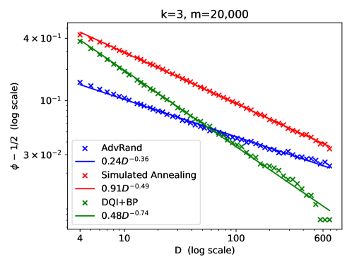
Figure 4: On the Gallager’s ensemble at $m=20,000$ constraints, we compare the fraction $\phi$ of variables satisfied in the solutions found by AdvRand and simulated annealing. We fix $k$, the number of variables in each constraint at $3$ and we vary $D$, the number of constraints that each variable is contained in, from $4$ to $687$. The lines display the linear least-square fits to the log-log plot of $\phi-1/2$ versus $D$.

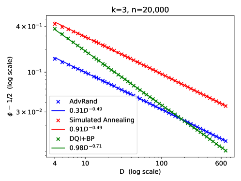
Figure 5: On Gallager’s ensemble at $n=20,000$ variables, we compare the fraction $\phi$ of variables satisfied in the solutions found by AdvRand and simulated annealing. We fix $k$, the number of variables in each constraint at $3$ and we vary $D$, the number of constraints that each variable is contained in, from $4$ to $687$. The lines display the linear least-square fits to the log-log plot of $\phi-1/2$ versus $D$.

In [23] it was proven that, given max-$k$-XORSAT instances, AdvRand can in polynomial time find solutions satisfying a fraction $\frac{1}{2}+\frac{e^{-\mathcal{O}(k)}}{\sqrt{D}}$ of the constraints, even in the worst case, provided each variable is contained at most $D$ constraints. From figure 4 we observe that the average-case performance on Gallager’s ensemble in the constant-$m$ ensemble with $k=3$ appears to have much better scaling with $D$ than this worst-case bound and, perhaps surprisingly, also better scaling with $D$ than simulated annealing. Specifically, our curvefits find that simulated annealing yields $\phi_{\mathrm{SA}}\simeq\frac{1}{2}+\frac{0.91}{D^{0.49}}$ and AdvRand yields $\phi_{\mathrm{AR}}\simeq\frac{1}{2}+\frac{0.24}{D^{0.36}}$. Extrapolating these fits suggests that AdvRand should achieve better approximate optima than simulated annnealing once $D$ surpasses roughly $3\times 10^{4}$. In these simulated annealing experiments we vary $\beta$ linearly from 0 to $3$ and apply $5,000$ sweeps through the variables, i.e. $5,000n=10^{8}$ Metropolis updates.

9.4 Algebraic Attacks Based on List Recovery

For the our OPI instances, we believe that the most credible classical algorithms to consider as competitors to DQI on these problem instances must be attacks that exploit their algebraic structure.

The max-LINSAT problem can be viewed as finding a codeword from $C$ that approximately maximizes $f$. With DQI we have reduced this to a problem of decoding $C^{\perp}$ out to distance $\ell$. For a Reed-Solomon code, as defined in (11), its dual is also a Reed-Solomon code. Hence, both $C$ and $C^{\perp}$ can be efficiently decoded out to half their distances, which are $m-n+1$ and $n+1$, respectively. However, max-LINSAT is not a standard decoding problem, i.e. finding the nearest codeword to a given string under the promise that the distance to the nearest string is below some bound. In fact, exact maximum-likelihood decoding for general Reed-Solomon codes with no bound on distance is known to be NP-hard [48].

The OPI problem is very similar to a problem studied in the coding theory literature known as list-recovery, applied in particular to Reed-Solomon codes. In list-recovery, for a code $C\subseteq\mathbb{F}_{p}^{m}$, one is given sets $F_{0},F_{1},\ldots,F_{m-1}\subseteq\mathbb{F}_{p}$ (which correspond to our sets $f_{i}^{-1}(+1)$), and asked to return all codewords $c\in C$ so that $c_{i}\in F_{i}$ for as many $i$ as possible. It is easy to see that solving this problem for Reed-Solomon codes will solve the OPI problem, assuming the list of all matching codewords is small. However, existing list-recovery algorithms for Reed-Solomon codes rely on the size of the $F_{i}$ being quite small (usually constant, relative to $m$) and do not apply in this parameter regime. In particular, the best known list-recovery algorithm for Reed-Solomon codes is the Guruswami-Sudan algorithm [49]; but this algorithm breaks down when the size of the $|F_{i}|$ is larger than $m/n$ (this is the Johnson bound for list-recovery). In our setting, $|F_{i}|=p/2\approx m/2$, which is much larger than $m/n\approx 10$. Thus, the Guruswami-Sudan algorithm does not apply. Moreover, we remark that in this parameter regime, if the $f_{i}$ are random, we expect there to be exponentially many codewords satisfying all of the constraints; this is very different from the coding-theoretic literature on list-recovery, which generally tries to establish that the number of such codewords is at most polynomially large in $m$, so that they can all be returned efficiently. Thus, standard list-recovery algorithms are not applicable in the parameter regime we consider.

9.5 Lattice-Based Heuristics

A problem similar to our Optimal Polynomial Intersection problem—but in a very different parameter regime—has been considered before, and has been shown to be susceptible to lattice attacks. In more detail, in the work [12], Naor and Pinkas proposed essentially the same problem, but in the parameter regime where $p$ is exponentially large compared to $m$, and where $|f_{i}^{-1}(+1)|\ll p/2$ is very small (in particular, not balanced, like we consider). The work [12] conjectured that this problem was (classically) computationally difficult. This conjecture was challenged by Bleichenbacher and Nguyen in [13] using a lattice-based attack, which we describe in more detail below. However, this lattice-based attack does not seem to be effective—either in theory or in practice—against our OPI problem. Intuitively, one reason is that in the parameter regime that the attack of [13] works, a solution to the max-LINSAT problem—which will be unique with high probability—corresponds to a unique shortest vector in a lattice, which can be found via heuristic methods. In contrast, in our parameter regime, there are many optimal solutions, corresponding to many short vectors; moreover, empirically it seems that there are much shorter vectors in the appropriate lattice that do not correspond to valid solutions. Thus, these lattice-based methods do not seem to be competitive with DQI for our problem.

The target of the attack in [13] is syntactically the same as our problem, but in a very different parameter regime. Concretely, $p$ is chosen to be much larger than $m$ or $n$, while the size $r:=|f_{i}^{-1}(+1)|$ of the set of “allowed” symbols for each $i=1,\ldots,m$ is very small. (Here, we assume that $f_{i}^{-1}(+1)$ has the same size $r$ for all $i$ for simplicity of presentation; this can be relaxed). In [13], the $f_{i}$’s are chosen as follows. Fix a planted solution $\mathbf{x}^{*}$, and set the $f_{i}$ so that $f_{i}(\mathbf{b}_{i}\cdot\mathbf{x}^{*})=1$ for all $i$; thus $f(\mathbf{x}^{*})=m$. Then for each $i$, $f_{i}(y)$ is set to $1$ for a few other random values of $y\in\mathbb{F}_{p}$, and $f_{i}(z)=-1$ for the remaining $z\in\mathbb{F}_{p}$. With high probability, $\mathbf{x}^{*}$ is the unique vector with large objective value, and the problem is to find it.

In our setting, where $r=|f_{i}^{-1}(+1)|\approx p/2$, $m=p-1$ and $n=\lceil m/10\rfloor$, we expect there to be many vectors $\mathbf{x}$ with $f(\mathbf{x})=m$ when the $f_{i}$ are random. We have seen that DQI can find a solution with $f(\mathbf{x})\approx 0.7179m$ (even for arbitrary $f_{i}$).

The way the attack of [13] works in our setting is the following. For $\mathbf{x}\in\mathbb{F}_{p}^{n}$, define a polynomial $P_{\mathbf{x}}(Z)=\sum_{j=1}^{n}x_{j}Z^{j-1}$. Let $F_{i}=f_{i}^{-1}(+1)$, and write $F_{i}=\{v_{i,1},v_{i,2},\ldots,v_{i,r}\}\subseteq\mathbb{F}_{p}$. If $f(\mathbf{x})=m$, then $P_{\mathbf{x}}(\gamma^{i})\in F_{i}$ for all $i=1,\ldots,m$, where we recall from §2.2 that $\gamma$ is a primitive element of $\mathbb{F}_{p}$, and $B_{i,j}=\gamma^{ij}$. Let $L_{i}(Z)=\prod_{j\neq i}\frac{Z-\gamma^{j}}{\gamma^{i}-\gamma^{j}}.$ By Lagrange interpolation, we have

$$P_{\mathbf{x}}(Z)=\sum_{i=1}^{m}P_{\mathbf{x}}(\gamma^{i})L_{i}(Z)=\sum_{i=1}^{m}\left(\sum_{j=1}^{r}\delta_{i,j}^{(P)}\ v_{i,j}\right)L_{i}(Z),$$ (211)

where $\delta_{i,j}^{(P)}$ is $1$ if $P_{\mathbf{x}}(\gamma^{i})=v_{i,j}$ and $0$ otherwise. Since $P_{\mathbf{x}}(Z)$ has degree at most $n-1$, the coefficients on $Z^{k}$ are equal to zero for $k=n,n+1,\ldots,p-1$. Hence, (211) gives us $p-n=m-n+1$ $\mathbb{F}_{p}$-linear constraints on the vector $\bm{\delta}\in\{0,1\}^{rm}$ that contains the $\delta_{i,j}^{(P)}$’s. Collect these constraints in a matrix $A\in\mathbb{F}_{p}^{m-n+1\times rm}$, so that $A\bm{\delta}=0$. Consider the lattice $\Lambda:=\{\bm{\delta}^{\prime}\in\mathbb{Z}^{rm}\,|\,A\bm{\delta}^{\prime}=0\mod p\}.$ Our target vector $\bm{\delta}$ clearly lies in $\Lambda$, and moreover it has a very short $\ell_{2}$ norm: $\|\bm{\delta}\|_{2}=\sqrt{m}$. Thus, we may hope to find it using methods like LLL [51] or Schnorr’s BKZ reduction [52, 53], and this is indeed the attack. Upon finding a vector $\bm{\delta}$ of the appropriate structure (namely, so that $\delta_{i,j}^{(P)}=1$ for exactly one $j\in\{1,\ldots,r\}$ for each $i$), we may read off the evaluations of $P_{\mathbf{x}}$ from the $F_{i}$, and hence recover $\mathbf{x}$.

Bleichenbacher and Nguyen show that in some parameter regimes, the target vector $\bm{\delta}$ with length $\sqrt{m}$ is likely to be the shortest vector in $\Lambda$. However, these parameter regimes are very different from ours. For example, their results hold for $p\approx 2^{80}$, and $r\leq 16$, with codes of rate $n/m$ at least $0.88$. In contrast, in our setting we have much larger lists, with $r\approx p/2$, and much lower-rate codes, with $n/m\approx 1/10$ (although in [13], they take $m,n\ll p$ while we take $m\approx p$, so this is not a direct comparison).

Empirically, this attack does not seem to work in our parameter regime. Indeed, the lattice heuristics do find short vectors in the lattice $\Lambda$, but these vectors are much shorter than $\sqrt{m}$ whenever $m$ and $n_{\text{distractors}}$ are comparable to $p$ (see Figure 6). As a consequence, the success probability when applied to our OPI instances appears to decay exponentially with $p$.

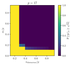
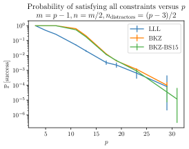
Figure 6: The attack of Bleichenbacher and Nguyen [13] is workable when the shortest nonzero vector in a particular lattice has weight $\sqrt{m}$. Above, left, we apply the BKZ algorithm [53] to find the shortest nonzero vector (under the 2-norm) in the lattices arising from random problem instances for various $m$ and $n_{\text{distractors}}.$ We observe that the shortest vector almost always has 2-norm $<\sqrt{m}$ in the regime where $m$ and $n_{\text{distractors}}$ are both a significant fraction of $p$. Consequently, the success probability of the attack when applied to our OPI problem in the regime where $m=p-1,n=m/2,n_{\text{distractors}}=(p-3)/2$ appears to exhibit exponential decay with $p$ whether LLL, BKZ with a block size of 15 (“BKZ-15”) or BKZ with unlimited block size. In this regime we believe the lattice-based heuristic of [13] does not succeed.

10 Beating Simulated Annealing on max-XORSAT

In this section we construct a class of max-XORSAT instances such that DQI, using belief propagation decoders, achieves a better approximation than we are able to achieve using simulated annealing. DQI+BP also achieves a better approximation than we obtain from any of the other general-purpose optimization heuristics that we try: greedy optimization, the truncation heuristic, and AdvRand. However, we do not claim this as an example of quantum advantage because we are able to also construct a classical heuristic tailored to the class of instances which still beats the approximation achieved by DQI+BP.

Given a max-XORSAT instance $B\mathbf{x}\stackrel{{\scriptstyle\max}}{{=}}\mathbf{v}$, the degree of a variable is the number of constraints in which it is contained. The degree of a constraint is the number of variables that are contained in it. Hence, the degree of the $i^{\textrm{th}}$ constraint is the number of nonzero entries in the $i^{\textrm{th}}$ row of $B$ and the degree of the $j^{\textrm{th}}$ variable is the number nonzero entries in the $j^{\textrm{th}}$ column of $B$. For an LDPC code, the degree of a parity check is the number of bits that it contains, and the degree of a bit is the number of parity checks in which it is contained. These degrees correspond to the number of nonzero entries in the rows and columns of the parity check matrix.

Given a max-XORSAT instance, let $\Delta_{j}$ be the fraction of variables that have degree $j$. Let $\kappa_{i}$ be the fraction of constraints that have degree $i$. Via DQI, a max-XORSAT instance with degree distribution $\Delta$ for the variables and $\kappa$ for the constraints is reduced to a decoding problem for a code with degree distribution $\Delta$ for the parity checks and $\kappa$ for the bits. For regular LDPC codes, in which every bit has degree $k$ and every constraint has degree $D$, the error rate from which belief propagation can reliably decode deteriorates as $D$ increases. However, it has been discovered that belief propagation can still work very well for certain irregular codes in which the average degree $\bar{D}$ of the parity checks is large [54]. In contrast, we find that the approximate optima achieved by simulated annealing on the corresponding irregular max-XORSAT instances of average degree $\bar{D}$ are typically no better than on regular instances in which every variable has degree exactly $\bar{D}$. This allows us to find examples where DQI achieves a better approximation than simulated annealing.

If the $m$ bits in an LDPC code have degree distribution $\kappa$ the total number of nonzero entries in the parity check matrix is $m\sum_{i}i\kappa_{i}$. If the $n$ parity checks in an LDPC code have degree distribution $\Delta$ then the total number of nonzero entries in the parity check matrix is $n\sum_{j}j\Delta_{j}$. Hence to define a valid LDPC code, a pair of degree distributions must satisfy

$$\textstyle{\sum_{i=1}^{m}\kappa_{i}} = 1$$ (212)

$$\textstyle{\sum_{j=1}^{n}\Delta_{j}} = 1$$ (213)

$$\textstyle{m\sum_{i=1}^{m}i\kappa_{i}} = \textstyle{n\sum_{j=1}^{n}j\Delta_{j}}.$$ (214)

Given any $\kappa_{1},\ldots,\kappa_{m}$ and $\Delta_{1},\ldots,\Delta_{n}$ satisfying these constraints, it is straightforward to sample uniformly from the set of all parity check matrices with $m$ bits whose degree distribution is $\kappa$ and $n$ parity checks whose degree distribution is $\Delta$. Furthermore, the maximum error rate from which belief propagation can reliably correct on codes from this ensemble can be computed in the limit of $m\to\infty$ by a method called density evolution, which numerically solves for the fixed point of a certain stochastic process [20]. Using this asymptotic maximum error rate as an objective function, one can optimize degree distributions to obtain irregular LDPC codes that outperform their regular counterparts [54].

As a concrete example, we consider the degree distribution shown in Figure 7.

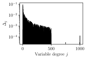
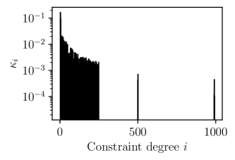
Figure 7: Degree distribution for an irregular instance sampled with $m=50,000$ and $n=31,216$. The full table of variable and constraint degrees is available in Appendix E.

After generating a random max-XORSAT instance with 50,000 constraints and 31,216 variables consistent with this degree distribution we find that belief propagation can achieve decoding with $99.5\%$ reliability at bit flip error rate $6,437/50,000$, which is close to the asymptotic threshold of $\approx 13\%$ predicted by density evolution. Assuming Conjecture 7.1, we thus have Corollary 7.1 which states that DQI can asymptotically find solutions that satisfy $0.8346m$ constraints with high probability. In contrast, when we run simulated annealing on this instance with $10^{6}$ sweeps, in sixteen trials the fraction of satisfied constraints ranges from $0.81024$ to $0.81488$. The truncation heuristic would be predicted to achieve approximately $0.8122$, and experimentally we saw $0.8124$. The greedy algorithm performs far worse than simulated annealing on this instance. In sixteen trials its best satisfaction fraction was $0.666$. Our trial of AdvRand achieved $0.5536$.

The following classical algorithm can exceed the approximation achieved by DQI+BP on the above example, by exploiting the highly unbalanced degree distribution of its constraints. We modify simulated annealing (which is described in Section 9.1) by adding a $\beta$-dependent factor to each term in the cost function. Letting $n_{i}$ denote the number of variables contained in constraint $i$, we use the cost function

$$f^{(\beta)}(\mathbf{x})=\sum_{i=1}^{m}\max\left(0,1-e^{-\beta/n_{i}}\right)f_{i}\left(\sum_{j=1}^{n}B_{ij}x_{j}\right).$$ (215)

We apply 1 million sweeps (since there are $50,000$ constraints this corresponds to fifty billion Metropolis updates), interpolating linearly from $\beta=0$ to $\beta=5$. After this, we are left with solutions that satisfy approximately $0.88m$ clauses. We call this algorithm irregular annealing since it takes advantage of the irregularity of the instance prioritizing the lower-degree constraints early in the annealing process.

11 DQI for Folded Codes and over Extension Fields

In §5, we describe the DQI algorithm for the max-LINSAT problem over prime fields. However, DQI works over extension fields as well, and also works for so-called folded codes. In this section, we go through the details to extend DQI to these settings. Our main motivation is to show that DQI is applicable to the problem considered by Yamakawa and Zhandry in [17], which is similar to our OPI problem, but for folded Reed-Solomon codes. Moreover, as discussed in §3, if a variant of theorem 2.1 applies in the regime studied by Yamakawa and Zhandry, then equation (7) implies that DQI can find a solution satisfying all constraints.

11.1 Folded max-LINSAT problem

In [17], Yamakawa and Zhandry define the following oracle problem, which they prove can be solved in polynomially many queries by a quantum computer but requires exponentially many queries for classical computers.

Definition 11.1.

Fix a prime power $q$ and integers $m,n,r$ such that $r$ divides $m$ and $m>n$. Let $\mathcal{O}:\{1,\ldots,m/r\}\times\mathbb{F}_{q}^{r}\to\{0,1\}$ be a random function. Let $B\in\mathbb{F}_{q}^{m\times n}$ be a Vandermonde matrix (so that $B_{i,j}=\gamma^{ij}$ for $i\in\{0,\ldots,m-1\}$, $j\in\{0,\ldots,n-1\}$ where $\gamma$ is a primitive element of $\mathbb{F}_{q}$), written as

$$B=\left[\begin{array}[]{c}B_{1}\\ \hline\cr B_{2}\\ \hline\cr\vdots\\ \hline\cr B_{m/r}\end{array}\right]$$ (216)

where $B_{i}\in\mathbb{F}_{q}^{r\times n}$. The Yamakawa-Zhandry problem is, given $B$ and query access to $\mathcal{O}$, to efficiently find $\mathbf{x}\in\mathbb{F}_{q}^{n}$ such that $\mathcal{O}(i,B_{i}\mathbf{x})=1$ for all $i\in\{1,\ldots,m/r\}.$

The problem in definition 11.1 has some similarities to definition 2.1, and especially to our OPI example in Section 2.2, but is not exactly the same, as the problem in definition 11.1 is for folded Reed-Solomon codes, over an extension field $\mathbb{F}_{q}$. Below, we extend DQI to this setting. More precisely, we consider the following generalization of Definition 2.1.

Definition 11.2 (Folded max-LINSAT).

Let $\mathbb{F}_{q}$ be a finite field, where $q$ is any prime power. For $i=1,\ldots,m/r$, let $f_{i}:\mathbb{F}_{q}^{r}\to\{+1,-1\}$ be arbitrary functions. Given a matrix $B\in\mathbb{F}_{q}^{m\times n}$, write $B$ as

$$B=\left[\begin{array}[]{c}B_{1}\\ \hline\cr B_{2}\\ \hline\cr\vdots\\ \hline\cr B_{m/r}\end{array}\right]$$ (217)

where $B_{i}\in\mathbb{F}_{q}^{r\times n}$. Given such a $B$, the $r$-folded max-LINSAT problem is to find $\mathbf{x}\in\mathbb{F}_{q}^{n}$ maximizing the objective function

$$f(\mathbf{x})=\sum_{i=1}^{m/r}f_{i}(B_{i}\mathbf{x}).$$ (218)

We now describe how to adapt the presentation in §5.2 to the folded max-LINSAT problem. As before, we first discuss the properties of the DQI state $|P(f)\rangle:=\sum_{\mathbf{x}\in\mathbb{F}_{p}^{n}}P(f(\mathbf{x}))|\mathbf{x}\rangle$ and then describe the algorithm for creating it.

Again, mirroring §5.2, we assume that $2\ell+1<d^{\perp}$ where $d^{\perp}$ is the minimum distance of the folded code $C^{\perp}=\{\mathbf{d}\in\mathbb{F}_{q}^{m}:B^{T}\mathbf{d}=\mathbf{0}\}$. Note that folding affects the definition of $d^{\perp}$. In a folded code, we view every codeword $\mathbf{y}\in\mathbb{F}_{q}^{m}$ as an $m/r$-tuple $(\mathbf{y}_{1},\ldots\mathbf{y}_{m/r})$ of elements of $\mathbb{F}_{q}^{r}$ and regard each $\mathbf{y}_{i}$ as a symbol. Consequently, the Hamming weight $|.|:\mathbb{F}_{q}^{m}\to\{0,\ldots,m/r\}$ associated with the folded code is the number of $\mathbf{y}_{i}$ not equal to $\mathbf{0}\in\mathbb{F}_{q}^{r}$.

11.2 DQI Quantum State for Folded max-LINSAT

As in §5.2, we assume that no $f_{i}$ is constant and that the preimages $F_{i}:=f_{i}^{-1}(+1)$ have the same cardinality for all $i=1,\ldots,m/r$. This allows us to define $g_{i}$ as $f_{i}$ shifted and rescaled so that its Fourier transform

$$\tilde{g}_{i}(\mathbf{y})=\frac{1}{\sqrt{q^{r}}}\sum_{\mathbf{x}\in\mathbb{F}_{q}^{r}}\omega_{p}^{\mathrm{tr}(\mathbf{y}\cdot\mathbf{x})}g_{i}(\mathbf{x}),$$ (219)

where $\mathrm{tr}:\mathbb{F}_{q}\to\mathbb{F}_{p}$ is the field trace, vanishes at $\mathbf{y}=\mathbf{0}\in\mathbb{F}_{q}^{r}$ and is normalized, i.e. $\sum_{\mathbf{x}\in\mathbb{F}_{q}^{r}}|g_{i}(\mathbf{x})|^{2}=\sum_{\mathbf{y}\in\mathbb{F}_{q}^{r}}|\tilde{g}_{i}(\mathbf{y})|^{2}=1$. More explicitly, we define

$$g_{i}(\mathbf{x}):=\frac{f_{i}(\mathbf{x})-\overline{f}}{\varphi}$$ (220)

where $\overline{f}:=\frac{1}{q^{r}}\sum_{\mathbf{x}\in\mathbb{F}_{q}^{r}}f_{i}(\mathbf{x})$ and $\varphi:=\left(\sum_{\mathbf{y}\in\mathbb{F}_{q}^{r}}|f_{i}(\mathbf{y})-\overline{f}|^{2}\right)^{1/2}$. The sums $f(\mathbf{x})=\sum_{i=1}^{m/r}f_{i}(B_{i}\mathbf{x})$ and $g(\mathbf{x})=\sum_{i=1}^{m/r}g_{i}(B_{i}\mathbf{x})$ are related by $f(\mathbf{x})=g(\mathbf{x})\varphi+m\overline{f}$. Substituting this relationship for $f$ in $P(f)$, we obtain an equivalent polynomial $Q(g)$ which, by Lemma A.1 in appendix A, can be expressed as a linear combination of elementary symmetric polynomials $P^{(k)}$

$$Q(g(\mathbf{x})):=\sum_{l=0}^{\ell}u_{k}P^{(k)}\left(g_{1}(B_{1}\mathbf{x}),\ldots,g_{m/r}(B_{m/r}\mathbf{x})\right).$$ (221)

We will write the DQI state

$$|P(f)\rangle=\sum_{\mathbf{x}\in\mathbb{F}_{q}^{n}}P(f(\mathbf{x}))|\mathbf{x}\rangle=\sum_{\mathbf{x}\in\mathbb{F}_{q}^{n}}Q(g(\mathbf{x}))|\mathbf{x}\rangle=|Q(g)\rangle$$ (222)

as a linear combination of $|P^{(0)}\rangle,\ldots,|P^{(\ell)}\rangle$ defined as

$$\ket{P^{(k)}}:=\frac{1}{\sqrt{q^{n-rk}{m/r\choose k}}}\sum_{\mathbf{x}\in\mathbb{F}_{q}^{n}}P^{(k)}\left(g_{1}(B_{1}\mathbf{x}),\ldots,g_{m/r}(B_{m/r}\mathbf{x})\right)\ket{\mathbf{x}}.$$ (223)

By definition,

$$P^{(k)}(g_{1}(B_{1}\mathbf{x}),\ldots,g_{m/r}(B_{m/r}\mathbf{x})) = \sum_{\begin{subarray}{c}i_{1},\ldots,i_{k}\\ \mathrm{distinct}\end{subarray}}\prod_{i\in\{i_{1},\ldots,i_{k}\}}g_{i}(B_{i}\mathbf{x})$$ (224)

$$= \sum_{\begin{subarray}{c}i_{1},\ldots,i_{k}\\ \mathrm{distinct}\end{subarray}}\prod_{i\in\{i_{1},\ldots,i_{k}\}}\left(\frac{1}{\sqrt{q^{r}}}\sum_{\mathbf{y}_{i}\in\mathbb{F}_{q}^{r}}\omega_{p}^{-\mathrm{tr}(\mathbf{y}_{i}\cdot B_{i}\mathbf{x})}\ \tilde{g}_{i}(\mathbf{y}_{i})\right)$$ (225)

$$= \sum_{\begin{subarray}{c}\mathbf{y}\in\mathbb{F}_{q}^{m}\\ |\mathbf{y}|=k\end{subarray}}\frac{1}{\sqrt{q^{rk}}}\ \omega_{p}^{-\mathrm{tr}((B^{T}\mathbf{y})\cdot\mathbf{x})}\ \prod_{\begin{subarray}{c}i=1\\ \mathbf{y}_{i}\neq 0\end{subarray}}^{m/r}\tilde{g}_{i}(\mathbf{y}_{i})$$ (226)

where $|.|:\mathbb{F}_{q}^{m}\to\{0,\ldots,m/r\}$ is the Hamming weight associated with the folded code. From (226) we see that the Quantum Fourier Transform of $\ket{P^{(k)}}$ is

$$|\widetilde{P}^{(k)}\rangle:=F^{\otimes n}|P^{(k)}\rangle=\frac{1}{\sqrt{\binom{m/r}{k}}}\sum_{\begin{subarray}{c}\mathbf{y}\in\mathbb{F}_{q}^{m}\\ |\mathbf{y}|=k\end{subarray}}\left(\prod_{\begin{subarray}{c}i=1\\ \mathbf{y}_{i}\neq 0\end{subarray}}^{m/r}\tilde{g}_{i}(\mathbf{y}_{i})\right)|B^{T}\mathbf{y}\rangle.$$ (227)

As in §5.2, if $|\mathbf{y}|<d^{\perp}/2$, then $B^{T}\mathbf{y}$ are all distinct and $\ket{P^{(0)}},\ldots,\ket{P^{(\ell)}}$ form an orthonormal set. Consequently,

$$\ket{P(f)}=\sum_{k=0}^{\ell}w_{k}\ket{P^{(k)}}$$ (228)

where

$$w_{k}=u_{k}\sqrt{q^{n-rk}\binom{m/r}{k}},$$ (229)

and $\langle P(f)|P(f)\rangle=\|\mathbf{w}\|^{2}$.

11.3 DQI Algorithm for Folded max-LINSAT

Similarly to DQI for general max-LINSAT, the algorithm for folded max-LINSAT uses four quantum registers: a weight register comprising $\lceil\log_{2}\ell\rceil$ qubits, a mask register with $m/r$ qubits, an error register with $m\lceil\log_{2}q\rceil$ qubits, and a syndrome register with $nr\lceil\log_{2}q\rceil$ qubits. We will consider the error and syndrome registers as consisting of $m/r$ and $n$ subregisters, respectively, where each subregister consists of $r\lceil\log_{2}q\rceil$ qubits.

We begin by initializing the weight register in the normalized state $\sum_{k=0}^{\ell}w_{k}\ket{k}$. Next, we prepare the mask register in the Dicke state corresponding to the weight register

$$\to\sum_{k=0}^{\ell}w_{k}\ket{k}\frac{1}{\sqrt{\binom{m/r}{k}}}\sum_{\begin{subarray}{c}\bm{\mu}\in\{0,1\}^{m/r}\\ |\bm{\mu}|=k\end{subarray}}\ket{\mathbf{\bm{\mu}}}.$$ (230)

Let $G_{i}$ denote a unitary acting on $r\lceil\log_{2}q\rceil$ qubits that sends $\ket{\mathbf{0}}$ to

$$\sum_{\mathbf{c}_{i}\in\mathbb{F}_{q}^{r}}\tilde{g}_{i}(\mathbf{c}_{i})\ket{\mathbf{c}_{i}},$$ (231)

We apply $G_{i}$ to the $i^{\textrm{th}}$ subregister of the error register conditional on the $i^{\textrm{th}}$ qubit in the mask register, which yields

$$\to\sum_{k=0}^{\ell}w_{k}\ket{k}\frac{1}{\sqrt{\binom{m/r}{k}}}\sum_{|\bm{\mu}|=k}\ket{\bm{\mu}}\prod_{i=1}^{m/r}G_{i}^{\mu_{i}}\ket{\mathbf{0}}^{\otimes m}$$ (232)

$$=\sum_{k=0}^{\ell}w_{k}\ket{k}\frac{1}{\sqrt{\binom{m/r}{k}}}\sum_{|\bm{\mu}|=k}\ket{\bm{\mu}}\sum_{\mathbf{c}\in\mathbb{F}_{q}^{rk}}\tilde{g}_{\mu(1)}(\mathbf{c}_{1})\ldots\tilde{g}_{\mu(k)}(\mathbf{c}_{k})\ket{\mathbf{c}\hookrightarrow\bm{\mu}}$$ (233)

where $\mu_{i}$ denotes the $i^{\textrm{th}}$ entry of $\bm{\mu}$, $\mu(j)$ denotes the index of the $j^{\textrm{th}}$ nonzero entry of $\bm{\mu}$, and $\mathbf{c}\hookrightarrow\bm{\mu}$ denotes the string in $\mathbb{F}_{p}^{m}$ obtained by substituting the $j^{\textrm{th}}$ entry of $\mathbf{c}=(\mathbf{c}_{1},\ldots,\mathbf{c}_{k})$ for the $j^{\textrm{th}}$ nonzero entry in $\bm{\mu}$ and setting the other entries to $\mathbf{0}\in\mathbb{F}_{q}^{r}$. (For example $(\mathbf{c}_{1},\mathbf{c}_{2},\mathbf{c}_{3})\hookrightarrow 01011=(\mathbf{0},\mathbf{c}_{1},\mathbf{0},\mathbf{c}_{2},\mathbf{c}_{3})$.)

Next, we compute $B^{T}(\mathbf{c}\hookrightarrow\bm{\mu})$ into the syndrome register

$$\to\sum_{k=0}^{\ell}w_{k}\ket{k}\frac{1}{\sqrt{\binom{m/r}{k}}}\sum_{|\bm{\mu}|=k}\ket{\bm{\mu}}\sum_{\mathbf{c}\in\mathbb{F}_{q}^{rk}}\tilde{g}_{\mu(1)}(\mathbf{c}_{1})\ldots\tilde{g}_{\mu(k)}(\mathbf{c}_{k})\ket{\mathbf{c}\hookrightarrow\bm{\mu}}\ket{B^{T}(\mathbf{c}\hookrightarrow\bm{\mu})}.$$ (234)

But $\tilde{g}_{i}(\mathbf{0})=0$ for all $i$, so the values of $\mathbf{y}=\mathbf{c}\hookrightarrow\bm{\mu}$ appearing in the superposition are exactly the elements of $\{\mathbf{y}\in\mathbb{F}_{q}^{m}:|\mathbf{y}|=k\}$ where $|.|:\mathbb{F}_{q}^{m}\to\{0,\ldots,m/r\}$ is the Hamming weight associated with the folded code $C^{\perp}$. The content of the syndrome register is then $B^{T}\mathbf{y}$, and the task of finding $\mathbf{y}$ from $B^{T}\mathbf{y}$ is the bounded distance decoding problem on the folded code $C^{\perp}=\{\mathbf{y}\in\mathbb{F}_{q}^{m}:B^{T}\mathbf{y}=\mathbf{0}\}$. Moreover, $\mathbf{c}$ and $\bm{\mu}$ are uniquely determined by and easy to compute from $\mathbf{c}\hookrightarrow\bm{\mu}$. Consequently, uncomputing the content of the weight, mask, and error registers can be done efficiently whenever the bounded distance decoding problem on $C^{\perp}$ can be solved efficiently out to distance $\ell$.

Uncomputing disentangles the syndrome register from the other registers, leaving behind

$$\to \sum_{k=0}^{\ell}w_{k}\frac{1}{\sqrt{\binom{m/r}{k}}}\sum_{|\bm{\mu}|=k}\sum_{\mathbf{c}\in\mathbb{F}_{q}^{rk}}\tilde{g}_{\mu(1)}(\mathbf{c}_{1})\ldots\tilde{g}_{\mu(k)}(\mathbf{c}_{k})\ket{B^{T}(\mathbf{c}\hookrightarrow\bm{\mu})}$$ (235)

$$= \sum_{k=0}^{\ell}w_{k}\frac{1}{\sqrt{\binom{m/r}{k}}}\sum_{\begin{subarray}{c}\mathbf{y}\in\mathbb{F}_{q}^{m}\\ |\mathbf{y}|=k\end{subarray}}\left(\prod_{\begin{subarray}{c}i=1\\ \mathbf{y}_{i}\neq 0\end{subarray}}^{m/r}\tilde{g}_{i}(\mathbf{y}_{i})\right)\ket{B^{T}\mathbf{y}}$$ (236)

$$= \sum_{k=0}^{\ell}w_{k}\ket{\widetilde{P}^{(k)}}$$ (237)

which becomes the desired state $\ket{P(f)}$ after applying the Quantum Fourier Transform.

Appendix A Elementary Symmetric Polynomials

In this section we prove lemma A.1. Recall that our max-LINSAT cost function takes the form $f(\mathbf{x})=f_{1}(\mathbf{b}_{1}\cdot\mathbf{x})+\ldots+f_{m}(\mathbf{b}_{m}\cdot\mathbf{x})$, where $f_{j}:\mathbb{F}_{p}\to\{+1,-1\}$. Hence $f_{j}^{2}-1=0$ for all $j$. Consequently, the rescaled functions $g_{j}(x)=(f_{j}(x)-\overline{f})/\varphi$ also obey a quadratic identity that does not depend on $j$. (Namely, $\varphi^{2}g_{j}^{2}+2\overline{f}\varphi g+\overline{f}^{2}-1=0$.) Thus the conditions of lemma A.1 are met by both $f_{1},\ldots,f_{m}$ and $g_{1},\ldots,g_{m}$.

Lemma A.1.

Let $P$ be any degree-$\ell$ polynomial in a single variable. Let $x_{1},\ldots,x_{m}$ be variables that each obey a quadratic identity $ax_{j}^{2}+bx_{j}+c=0$, where $a,b,c$ are independent of $j$ and $a\neq 0$. Then $P(x_{1}+\ldots+x_{m})$ can be expressed as a linear combination of elementary symmetric polynomials: $P(x_{1}+\ldots+x_{m})=\sum_{k=0}^{\ell}u_{k}P^{(k)}(x_{1},\ldots,x_{m})$.

Proof.

Reducing modulo the quadratic identities:

$$ax_{j}^{2}+bx_{j}+c=0\quad j=1,\ldots,m$$ (238)

brings $P(x_{1}+\ldots+x_{m})$ into a form where none of $x_{1},\ldots,x_{m}$ is raised to any power greater than one. We can think of the resulting expression as a multilinear multivariate polynomial $P(x_{1},\ldots,x_{m})$, which is of total degree $\ell$. Since the coefficients in the $m$ identities described in (238) are independent of $j$, this multilinear multinomial is symmetric. That is, for any permutation $\pi\in S_{m}$ we have $P(x_{\pi(1)},\ldots,x_{\pi(m)})=P(x_{1},\ldots,x_{m})$. By the fundamental theorem of symmetric polynomials, multilinearity and symmetry together imply that the degree-$\ell$ polynomial $P(x_{1},\ldots,x_{m})$ can be expressed as a linear combination of elementry symmetric polynomials of degree at most $\ell$. ∎

Appendix B Gallager’s Ensemble

In [55] Gallager defined the following ensemble of matrices over $\mathbb{F}_{2}$. This ensemble is widely used in coding theory because when parity check matrices are drawn from Gallager’s ensemble, the resulting LDPC codes have good parameters with high probability. Together with a choice of $\mathbf{v}$, a matrix $B$ sampled from Gallager’s ensemble also induces a natural ensemble of $D$-regular max-$k$-XORSAT instances.

Given parameters $(k,D,b)$, a sample from Gallager’s ensemble of matrices $B\in\mathbb{F}_{2}^{bk\times bD}$ is generated as follows. Let $A$ denote the horizontal concatenation of $D$ identity matrices, each $b\times b$, yielding $A=[I_{1}I_{2}\ldots I_{D}]$. For $i=1,\ldots,k$ let $M_{i}=AP_{i}$ where $P_{1},\ldots,P_{k}$ are independent uniformly random $b\times b$ permutation matrices. Concatenate these vertically yielding

$$B^{T}=\left[\begin{array}[]{c}M_{1}\\ \hline\cr M_{2}\\ \hline\cr\vdots\\ \hline\cr M_{k}\end{array}\right]$$ (239)

The matrix $B^{T}$ thus has $n=bk$ rows and $m=bD$ columns, with $k$ ones in each row and $D$ ones in each column. By choosing each function $f_{1},\ldots,f_{m}$ independently at random to be either $f_{i}(x)=(-1)^{x}$ or $f_{i}(x)=-(-1)^{x}$ we obtain a $D$-regular instance of max-$k$-XORSAT as a special case of max-LINSAT over $\mathbb{F}_{2}$.

Gallager’s $(k,D,b)$ ensemble is not equivalent to sampling uniformly from all $bk\times bD$ matrices with $k$ ones in each row and $D$ ones in each column. It shares many properties with such a distribution but is more convenient to sample from.

Appendix C Simulated Annealing Applied to OPI

By the results of §9.1 we expect simulated annealing to yield solutions to the OPI instances of §2.2 where the fraction $\phi_{\max}$ of constraints satisfied scales like

$$\phi_{\max}\simeq\frac{1}{2}+\frac{c}{D^{\nu}}.$$ (240)

where $c$ and $\nu$ are free parameters of the fit. According to our crude theoretical model $\nu$ should be $1/2$. However, extrapolating from our empirical results with sparse instances we would expect $\nu$ to be slightly smaller than $1/2$. As shown in figure 8, experimental results match well to this prediction with $\nu=0.45$.

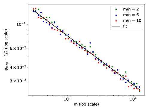
Figure 8: Here we generate OPI instances over $\mathbb{F}_{p}$ where $p$ takes prime values from $307$ to $12,343$. The number of constraints is $m=p-1$. For each $m$ we take $n\in\{m/2,m/6,m/10\}$, rounded to the nearest integer. We find that, independent of $n/m$, the approximation achieved by simulated annealing with $10,000$ sweeps fits well to $\phi_{\max}=1/2+1.8D^{-0.45}$.

Appendix D Heuristic Justification of Conjecture 7.1

In this appendix, we give a few arguments to explain why we believe that Conjecture 7.1 is plausible. Let

$$\zeta_{k}=\frac{1}{{m\choose k}}\sum_{\begin{subarray}{c}\mathbf{y}\in\mathbb{F}_{2}^{m}\\ |\mathbf{y}|=k\end{subarray}}\left|\left\{\mathbf{z}\in C^{\perp}\setminus\{0\}\,:\,|\mathbf{y}-\mathbf{z}|\leq\ell\right\}\right|.$$ (241)

Thus, our assumption in Conjecture 7.1 is that $\max_{k\leq\ell}\zeta_{k}=\zeta\leq 10^{-4}$. (Note that the $\ell$ in this appendix slightly differs from the use of $\ell$ in equation 133, by an additive factor of $+1$, to keep the statements in this section simple). Throughout this section, we recall that $C^{\perp}$ is the code $C^{\perp}=\{\mathbf{c}\in\mathbb{F}_{2}^{m}\,:\,B^{T}\mathbf{c}=0\}$, where $B^{T}\in\mathbb{F}_{2}^{n\times m}$ is a sparse random binary matrix as defined in §10.

As a zeroth heuristic argument, we note that a related quantity,

$$\mathbb{E}_{\mathbf{y}\in\mathbb{F}_{2}^{m}}\left|\left\{\mathbf{z}\in C^{\perp}\setminus\{0\}\,:\,|\mathbf{y}-\mathbf{z}|\leq\ell\right\}\right|$$ (242)

is clearly very small, by a simple counting argument. Indeed, for a completely random $\mathbf{y}\in\mathbb{F}_{2}^{m}$, the expected number of codewords of $C^{\perp}$ in a Hamming ball of radius $\ell$ about $\mathbf{y}$ is

$$\sum_{\mathbf{z}\in C^{\perp}}\Pr[|\mathbf{z}-\mathbf{y}|\leq\ell]=|C^{\perp}|\cdot\sum_{t\leq\ell}{m\choose t}\cdot 2^{-m}\approx 2^{m-n}\cdot 2^{mh(\ell/m)}\cdot 2^{-m},$$ (243)

where above we have used $|C^{\perp}|=2^{m-n}$ (assuming $B^{T}$ is full rank), and that the approximation that the volume of a Hamming ball in $\mathbb{F}_{2}^{m}$ of radius $\ell$ is approximately $2^{mh(\ell/m)}$, where $h(x)=-x\log_{2}(x)-(1-x)\log_{2}(1-x)$ is the binary entropy function. Plugging in $m=50,000$, $n=31,216$, and $\ell=6,437$ as in the example in §10, we see that this is approximately $2^{-22,000}$, which is very small indeed.

Of course, the quantity $\zeta_{k}$ is different from the quantity easily bounded above, as $\mathbf{y}$ is not a uniformly random vector, rather it is a random vector of weight $k\leq\ell$. In the following two sub-sections, we present heuristic arguments for why the above result should qualitatively still hold, even if $\mathbf{y}$ is chosen to be of weight $k\leq\ell$.

First, in §D.1, we give a more refined version of the counting argument above, which relies on a mild assumption about the expected weight distribution of $C^{\perp}$. We justify this assumption by showing that it holds for Gallager’s ensemble of LDPC codes, although our particular irregular ensemble seems difficult to analyze.

Next, in §D.2, we give an argument based on the assumptions that (a) $C^{\perp}$ has a decoder that works well on random errors, and (b) that $C^{\perp}$ is list-decodable up to radius $\ell$. We justify (a) by noting that it is true empirically, and again justify (b) by noting that it easily holds for Gallager’s ensemble of LDPC codes.

D.1 Argument from expected weight distribution

Let $A_{j}=|\{\mathbf{c}\in C^{\perp}\,:\,|\mathbf{c}|=j\}|$, and let $\alpha_{j}=\mathbb{E}_{C^{\perp}}A_{j}$, where the expectation is over the choice of code $C^{\perp}$, or equivalently over the choice of the matrix $B$. The assumption that we will base this heuristic argument on is that $\alpha_{j}$ is approximately binomial, in the sense that for all $j\in\{1,\ldots,m\}$

$$\alpha_{j}\leq 2^{-0.9n}{m\choose j}.$$ (244)

Note that $2^{-n}{m\choose j}$ is the value of $\alpha_{j}$ when $C^{\perp}$ is a random linear code  (that is, with a dense parity-check matrix), so (244) is asserting that $\alpha_{j}$ for a random LDPC code is not too much larger than that for a random linear code. While the full weight distribution of $C^{\perp}$ (for example, higher moments of the $A_{j}$) seems difficult to understand, an assumption like (244) on the first moments seems reasonable for random LDPC codes. As evidence for this, it is not hard to see that (244) holds for Gallager’s ensemble of LDPC codes as long as the degree is a sufficiently large constant. We include the argument below in §D.1.1 for completeness; see also [55]. The analysis in §D.1.1 suggests that Gallager’s ensemble with average check-degree of at least $8$ should easily satisfy (244), with $\frac{n}{m}=\frac{31,216}{50,000}$ (these are the parameters from our example in §10), provided that $n,m$ are sufficiently large.

Given the assumption (244), a counting argument shows that $\zeta$ is small with high probability. In more detail, let

$$Z_{k}=\sum_{\begin{subarray}{c}\mathbf{y}\in\mathbb{F}_{2}^{m}\\ |\mathbf{y}|=k\end{subarray}}\left|\left\{\mathbf{z}\in C^{\perp}\setminus\{0\}\,:\,|\mathbf{y}-\mathbf{z}|\leq\ell\right\}\right|,$$ (245)

so $\zeta_{k}=Z_{k}/{m\choose k}.$ Consider the number of times that any particular codeword $\mathbf{z}\in C^{\perp}$ of weight $j\geq 0$ contributes to $Z_{k}$. Such a $\mathbf{z}$ contributes to $Z_{k}$ once for each vector $\mathbf{y}$ of weight $k$ so that $|\mathbf{y}-\mathbf{z}|\leq\ell$. The number of these depends only on $j$, and is precisely

$$\sum_{t=\frac{k+j-\ell}{2}}^{k}{j\choose t}{m-j\choose k-t}.$$ (246)

To see this, notice that each such $\mathbf{y}$ is determined by the set $T=\mathrm{supp}(\mathbf{y})\cap\mathrm{supp}(\mathbf{z})$ and by the set $S=\mathrm{supp}(\mathbf{y})\cap\overline{\mathrm{supp}(\mathbf{z})}$. Let $t=|T|$. Then the requirement that $|\mathbf{y}-\mathbf{z}|\leq\ell$ is the same as the requirement that $(j-t)+(k-t)\leq\ell$, or that

$$t\geq\frac{k+j-\ell}{2}.$$ (247)

We also have $t\leq k$, as $T\subseteq\mathrm{supp}(\mathbf{y})$ and the latter has size $k$. Thus, to count the number of $\mathbf{y}$ that are counted for each such $\mathbf{z}$, we count the number of ways to choose $T$ and $S$, for each value of $t=|T|$ that satisfies $\frac{k+j-\ell}{2}\leq t\leq k$. There are ${j\choose t}$ ways to choose $t$ elements out of the $j$ in $\mathrm{supp}(\mathbf{z})$ to pick $T$; and there are ${m-j\choose k-t}$ ways to choose $k-t$ elements out of the $m-j$ in $\overline{\mathrm{supp}(\mathbf{z})}$ to pick $S$. Multiplying these together establishes the claim above.

We conclude that

$$\mathbb{E}_{C^{\perp}}[\zeta_{k}]\leq\frac{1}{{m\choose k}}\sum_{j=d^{\perp}}^{\ell+k}\alpha_{j}\sum_{t=\frac{k+j-\ell}{2}}^{k}{j\choose t}{m-j\choose k-t},$$ (248)

where the randomness is over the choice of the code $C^{\perp}$ (or equivalently, over the choice of the matrix $B$) from the ensemble in §10. If $\mathbb{E}_{C^{\perp}}[\zeta_{k}]\leq\eta$ for some small $\eta$, then Markov’s inequality will imply that

$$\Pr[\zeta_{k}>\zeta]\leq\frac{\eta}{\zeta},$$ (249)

and a union bound implies that

$$\Pr_{C^{\perp}}[\exists k\in\{1,\ldots,\ell\},\zeta_{k}>\zeta]\leq\frac{\ell\eta}{\zeta}.$$ (250)

To find such an $\eta$, we can numerically approximate (248), using our assumption (244). In order to do this cleanly, we first bound (248) by

$$\mathbb{E}_{C^{\perp}}[\zeta_{k}] \leq\frac{1}{{m\choose k}}\cdot(\ell+k)\max_{j\in\{\ell,\ldots\ell+k\}}\left[\alpha_{j}\cdot k\max_{t\in\left\{\frac{k+j-\ell}{2},\ldots,k\right\}}\left[{j\choose t}{m-j\choose k-t}\right]\right].$$ (251)

Taking logarithms and approximating the binomial coefficients ${x\choose y}\approx 2^{x\cdot h(y/x)}$, and plugging in

$$\log_{2}(\alpha_{j})\leq\log_{2}\left(2^{-0.9n}{m\choose j}\right)\approx-0.9n+m\cdot h\left(\frac{j}{m}\right),$$ (252)

we see that

$$\log_{2}(\mathbb{E}_{C^{\perp}}[\zeta_{k}]) \lesssim-m\cdot h\left(\frac{k}{m}\right)+\log_{2}(\ell+k)\ +$$ (253)

$$\max_{j\in\{\ell,\ldots,\ell+k\}}\left[\left(-0.9n+m\cdot h\left(\frac{j}{m}\right)\right)+\log_{2}(k)+\max_{t\in\left\{\frac{k+j-\ell}{2},\ldots,k\right\}}\left[j\cdot h\left(\frac{t}{j}\right)+(m-j)h\left(\frac{k-t}{m-j}\right)\right]\right].$$

This can be computed empirically for each $k$ (observing that it is maximized when $k=\ell$ is at its largest). In the example distribution of max-XORSAT that we consider in §10, we have:

$$m=50,000,\qquad n=31,216,\qquad\ell=6,437.$$

We see that for any $k$, eq. (253) gives a bound on $\log_{2}(\mathbb{E}_{C^{\perp}}[\zeta_{k}])\leq-360$, which implies that we may take $\eta$ in the above discussion to be $2^{-360}$, and hence (250) implies that

$$\Pr_{C^{\perp}}[\exists k\in\{1,\ldots,\ell\},\zeta_{k}>\zeta]\leq\frac{6437\cdot 2^{-360}}{2^{-300}}\leq 2^{-40}$$ (254)

when $\zeta=2^{-300}$, much smaller than the $10^{-4}$ we need in Conjecture 7.1).

D.1.1 Aside: Argument for (244) in Gallager’s ensemble

To illustrate why the assumption (244) seems plausible for the irregular ensemble of LDPC codes considered in §10, here we show that it holds for Gallager’s ensemble of LDPC codes [55]. We note that a bound on $\alpha_{j}$ is already present in [55], but we can use a simpler argument to get the relatively coarse bound that we need in (244); our argument here is also a simplification of an argument in [56]. To bound $\alpha_{j}=\mathbb{E}_{C^{\perp}}[A_{j}]$, it suffices to bound

$$P(j):=\Pr_{B^{T}}[B^{T}\mathbf{z}=0],$$ (255)

where $\mathbf{z}$ is any vector of weight $j$, and where $B^{T}\in\mathbb{F}_{2}^{n\times m}$ is the parity-check matrix for $C^{\perp}$. (Notice that since the distribution of $B^{T}$ is invariant under permutations of the columns, which vector $\mathbf{z}$ of weight $j$ we choose in the definition does not matter). Indeed, given $P(j)$, by linearity of expectation we have

$$\alpha_{j}=\mathbb{E}_{C^{\perp}}[A_{j}]={m\choose j}\cdot P(j).$$ (256)

Recall that in Gallager’s ensemble of LDPC codes (with degree $s$), the matrix $B^{T}$ is made up of $ns/m$ independent layers $M_{i}\in\mathbb{F}_{2}^{(m/s)\times m}$. Each layer $M_{i}$ is an independent random matrix so that each row has exactly $s$ ones, and so that the rows are disjoint. Let $F\in\mathbb{F}_{2}^{(m/s)\times m}$ be any such matrix, so that each $M_{i}$ is distributed like $F\Pi$ for a random permutation matrix $\Pi\in\mathbb{F}_{2}^{m\times m}$. Then for any vector $\mathbf{z}$ of weight $j$, the probability that $M_{i}\mathbf{z}=0$ is

$$\Pr[M_{i}\mathbf{z}=0]=\Pr_{\Pi}[F\Pi\mathbf{z}=0]=\Pr_{|\mathbf{y}|=j}[F\mathbf{y}=0],$$ (257)

where the probability in the final expression is over a random vector $\mathbf{y}$ of weight $j$. We can analyze this probability as

$$\Pr_{|\mathbf{y}|=j}[F\mathbf{y}=0] =\Pr_{\mathbf{y}\sim\mathrm{Ber}(j/m)^{m}}[F\mathbf{y}=0||\mathbf{y}|=j]$$ (258)

$$\leq\frac{\Pr_{\mathbf{y}\sim\mathrm{Ber}(j/m)^{m}}[F\mathbf{y}=0]}{\Pr_{\mathbf{y}\sim\mathrm{Ber}(j/m)^{m}}[|\mathbf{y}|=j]}$$ (259)

where $\mathrm{Ber}(j/m)$ is the Bernoulli distribution with mean $j/m$. We can bound the denominator by

$$\Pr_{\mathbf{y}\sim\mathrm{Ber}(j/m)^{m}}[|\mathbf{y}|=j]={m\choose j}(j/m)^{j}(1-j/m)^{j}=(1+o(1))\sqrt{\frac{m}{2\pi j(m-j)}}$$ (260)

using Stirling’s approximation. Thus,

$$\Pr_{|\mathbf{y}|=j}[F\mathbf{y}=0]\leq(1+o(1))\sqrt{\frac{2\pi j(m-j)}{m}}\Pr_{\mathbf{y}\sim\mathrm{Ber}(j/m)^{m}}[F\mathbf{y}=0].$$ (261)

When $\mathbf{y}\sim\mathrm{Ber}(j/m)^{m}$, the coordinates are independent; since the rows of $F$ have disjoint support, this means that the components of $F\mathbf{y}$ are also independent. Thus, we can bound the final term above by

$$\Pr_{\mathbf{y}\sim\mathrm{Ber}(j/m)^{m}}[F\mathbf{y}=0] =\left(\Pr_{u_{1},\ldots,u_{s}\sim\mathrm{Ber}(j/m)}\left[\sum_{i=1}^{s}u_{j}=0\right]\right)^{m/s}$$ (262)

$$=\left(\frac{1+(1-2j/m)^{s}}{2}\right)^{m/s}.$$ (263)

Finally, we use the fact that all of the layers are independent to conclude that

$$P(j)=\Pr_{B}[M_{i}\mathbf{z}=0]^{ns/m}\leq\left((1+o(1))\sqrt{\frac{2\pi j(m-j)}{m}}\right)^{ns/m}\left(\frac{1+(1-2j/m)^{s}}{2}\right)^{n}.$$ (264)

Thus, we have

$$\log_{2}(P(j))=-n\left(1-(1-2j/m)^{s}-\frac{s}{m}\log_{2}(C_{0}\sqrt{m})\right)$$ (265)

for some constant $C_{0}$. The final term is negligable compared to the second (for large $n,m$ with $n/m$ constant). Thus, as long as $s$ is large enough that, say, $(1-2j/m)^{s}<0.05$, we should safely have $P(j)\lesssim 2^{-0.9n}$. This implies that

$$\alpha_{j}\lesssim 2^{-0.9n}{m\choose j},$$ (266)

which was what we wanted. Plugging in parameters from our example in §10, $|1-2j/m|\leq|1-2\ell/m|\approx 0.743$, so the corresponding degree in Gallager’s ensemble would be about $s\approx 8$. This is much smaller than the average degree in our irregular example, although of course it is a different distribution.

D.2 Evidence based on list-decodability

As we have seen, for the $C^{\perp}$ in §10, there is a classical decoding algorithm that performs well (that is, succeeds with probability about $0.995$) against $\ell^{*}\approx 6437$ random errors (out of $m=50000$). In this section, we will prove the following lemma.

Lemma D.1.

Let $C^{\perp}\subseteq\mathbb{F}_{2}^{m}$ be a linear code of distance $d^{\perp}$, given by $C^{\perp}=\{\mathbf{z}\in\mathbb{F}_{2}^{m}\,:\,B^{T}\mathbf{z}=0\}$ for $B^{T}\in\mathbb{F}_{2}^{n\times m}$. Suppose that there is a syndrome decoding algorithm $\phi:\mathbb{F}_{2}^{n}\to\mathbb{F}_{2}^{m}$ so that $\Pr_{\mathbf{y}\sim\mathrm{Ber}(p^{*})^{m}}[\phi(B^{T}\mathbf{y})=\mathbf{y}]\geq 2/3$. Let $\epsilon>0$ and suppose that $\ell\leq(p^{*}-\epsilon)m$. Then

$$\Pr_{|\mathbf{y}|=\ell}[|\{\mathbf{z}\in C^{\perp}\setminus\{0\}\,:\,|\mathbf{z}-\mathbf{y}|\leq\ell\}|>0]\leq\eta,$$ (267)

where $\eta\leq\sqrt{m}\cdot\exp(-\Omega_{\epsilon,p^{*}}(-d^{\perp}))$, where the big-Omega notation suppresses dependence on $\epsilon$ and $p^{*}$.

Along with an additional assumption on $C^{\perp}$, namely that it is list-decodable up to radius $\ell$, Lemma D.1 gives evidence for Conjecture 7.1, as follows. Suppose that $C^{\perp}$ is $(\ell/m,L)$-list-decodable, which means that

$$\max_{\mathbf{y}\in\mathbb{F}_{2}^{m}}|\{\mathbf{z}\in C^{\perp}\,:\,|\mathbf{y}-\mathbf{z}|\leq\ell\}|\leq L,$$ (268)

for some $L=\mathrm{poly}(m)$. Suppose further that there is a decoding algorithm that works fairly well on error vectors $\mathbf{y}\sim\mathrm{Ber}(p^{*})^{m}$, for some $p^{*}$ that’s a bit larger than $\ell/m$, as in the hypothesis of Lemma D.1. (We know empirically that this is the case for the ensemble of codes $C^{\perp}$ given in §10). Then Lemma D.1 implies that

$$\frac{1}{{m\choose\ell}}\sum_{|\mathbf{y}|=\ell}\left|\left\{\mathbf{z}\in C^{\perp}\,:\,|\mathbf{y}-\mathbf{z}|\leq\ell\right\}\right|\leq\eta\cdot L,$$ (269)

which is exponentially small for sufficiently large $m$, assuming that $d^{\perp}$ scales linearly with $m$.

Thus, the assumptions of decent performance on the binary symmetric channel with crossover probability $p^{*}\approx\ell/m$, along with a list-decodability assumption, establishes Conjecture 7.1 for the case that $k=\ell$. We take this as evidence that the conjecture holds for all $k\leq\ell$. We note that the conjecture is trivially true for $k\leq d^{\perp}/2$, and we have given evidence that it holds for $k=\ell$, which in our example we estimate to be about $\ell\approx 0.8d^{\perp}$. Thus the gap is not very large, and it seems like the conjecture should only be easier to establish for smaller $k$. However, as we will see below (see Remark D.1), the proof of Lemma D.1 does not immediately work for $k<\ell$.

Before we prove Lemma D.1, we briefly address the plausibility of this list-decoding assumption. While we do not have a formal list-decoding result for the ensemble of LDPC codes considered in §10, there is a formal result for Gallager’s ensemble of LDPC codes [55]. In more detail, [56] showed that Gallager’s ensemble achieves list-decoding capacity, which means that it is list-decodable all the way up to radius approaching $d^{\perp}$ with a list size that is constant (independent of $m$). In our examples, $\ell$ is significantly smaller than $d^{\perp}$ (though larger than $d^{\perp}/2$), so our list-decodability assumption for the irregular ensemble of LDPC codes in §10 is significantly weaker than what is known to be true for Gallager’s ensemble.

In the rest of this section, we prove Lemma D.1. The high-level idea is that we will establish a threshold result (following the argument of [57]), which intuitively says that there is some threshold $\theta\in(0,1)$ so that if $\ell<\theta\cdot m$, then a random vector $\mathbf{y}$ of weight $\ell$ is extremely likely to be $\ell$-close to only the all-zero codeword; while if $\ell>\theta\cdot m$, then a random vector $\mathbf{y}$ of weight $\ell$ is extremely likely to have at least one other $\mathbf{z}\in C^{\perp}\setminus\{0\}$ within distance $\ell$. Since empirically decoding from $\ell$ errors succeeds with decent probability, this will imply that we are on the “good” side of the threshold, establishing (267). We now proceed with the details.

Proof of Lemma D.1.

For $r\geq 0$, let $\Omega_{r}=\{\mathbf{y}\in\mathbb{F}_{2}^{m}\,:\,|\mathcal{E}(\mathbf{y},|\mathbf{y}|+r)\cap(C^{\perp}\setminus\{0\})|>0\}$, where $\mathcal{E}(\mathbf{y},s)=\{\mathbf{x}\in\mathbb{F}_{2}^{m}\,:\,|\mathbf{y}-\mathbf{x}|\leq s\}$ is the Hamming ball of radius $s$ about $\mathbf{y}$. We make the following two observations about $\Omega_{r}$:

• $\Omega_{r}$ is decreasing, in the sense that if $\mathbf{y}\in\Omega_{r}$ and $\mathbf{x}\prec\mathbf{y}$, then $\mathbf{x}\in\Omega_{r}$, where we say that $\mathbf{x}\prec\mathbf{y}$ if $\mathrm{supp}(\mathbf{x})\subset\mathrm{supp}(\mathbf{y})$. To see this, suppose that $\mathbf{y}\in\Omega_{r}$, and let $\mathbf{x}=\mathbf{y}-\mathbf{e}_{i}$, where $i\in\mathrm{supp}(\mathbf{y})$ and $\mathbf{e}_{i}$ is the $i$’th standard basis vector. Suppose towards a contradiction that $\mathbf{x}\not\in\Omega_{r}$. Then there is some $\mathbf{c}\in C^{\perp}\setminus\{0\}$ so that $|\mathbf{c}-\mathbf{x}|\leq|\mathbf{x}|+r$. But then $|\mathbf{c}-\mathbf{y}|\leq|\mathbf{x}|+r+1=|\mathbf{y}|-1+r+1=|\mathbf{y}|+r$, contradicting the assumption that $\mathbf{y}\in\Omega_{r}$.

• Suppose that $\mathbf{y}\in\Omega_{r}$, and that there exists some $\mathbf{x}\not\in\Omega_{r}$ so that $|\mathbf{y}-\mathbf{x}|=1$. Then we claim that there are at least $d^{\perp}/2$ values of $\mathbf{x}^{\prime}\not\in\Omega_{r}$ (including $\mathbf{x}$) so that $|\mathbf{y}-\mathbf{x}^{\prime}|=1$. (Here, $d^{\perp}$ is the distance of the code $C^{\perp}$). To see this, let $\mathbf{c}\in C^{\perp}\setminus\{0\}$ be so that $|\mathbf{c}-\mathbf{x}|\leq|\mathbf{x}|+r$, as is guaranteed by the fact that $\mathbf{x}\not\in\Omega_{r}$. Then we must have $\mathbf{x}=\mathbf{y}+\mathbf{e}_{i}$ for some $i\in\mathrm{supp}(\mathbf{c})\setminus\mathrm{supp}(\mathbf{y})$. Indeed, $i$ can’t be in $\mathrm{supp}(\mathbf{y})$ because we have just shown that $\Omega_{r}$ is decreasing; and we must have $i\in\mathrm{supp}(\mathbf{c})$ because otherwise we would have $|\mathbf{c}-\mathbf{x}|=|\mathbf{c}-\mathbf{y}|+1>|\mathbf{y}|+r+1=|\mathbf{x}|+r$, a contradiction. Moreover, for any $i\in\mathrm{supp}(\mathbf{c})\setminus\mathrm{supp}(\mathbf{y})$, if $\mathbf{x}^{\prime}=\mathbf{y}+\mathbf{e}_{i}$, then $|\mathbf{c}-\mathbf{x}^{\prime}|\leq|\mathbf{x}^{\prime}|+r$. Thus, the number of such $\mathbf{x}^{\prime}$ is at least $|\mathrm{supp}(\mathbf{c})\setminus\mathrm{supp}(\mathbf{y})|$. We claim that this latter quantity is at least $d^{\perp}/2$. Indeed, since $\mathbf{c}$ is a nonzero codeword, we have

  $$d^{\perp}\leq|\mathbf{c}|=|\mathrm{supp}(\mathbf{c})\setminus\mathrm{supp}(\mathbf{y})|+|\mathrm{supp}(\mathbf{c})\cap\mathrm{supp}(\mathbf{y})|,$$

  and since $\mathbf{y}\in\Omega_{r}$, we have

  $$|\mathbf{y}|+r<|\mathbf{c}-\mathbf{y}|=|\mathrm{supp}(\mathbf{c})\setminus\mathrm{supp}(\mathbf{y})|+(|\mathbf{y}|-\mathrm{supp}(\mathbf{c})\setminus\mathrm{supp}(\mathbf{y})).$$

  Combining these two equations, we get

  $$|\mathrm{supp}(\mathbf{c})\setminus\mathrm{supp}(\mathbf{y})|>\frac{r+d^{\perp}}{2}\geq\frac{d^{\perp}}{2},$$

  as claimed.

With these two observations, we can apply Theorem 2.2 of [57] with $\Delta=d^{\perp}/2$. We conclude that there is some threshold $\theta_{r}\in(0,1)$ so that

$$\Pr_{\mathbf{y}\sim\mathrm{Ber}(p)^{m}}[\mathbf{y}\in\Omega_{r}]\begin{cases}\leq\Phi\left(\sqrt{d^{\perp}}\left(\sqrt{\ln(1/\theta_{r})}-\sqrt{\ln(1/p)}\right)\right)&\text{ if }\theta_{r}<p<1\\ \geq\Phi\left(\sqrt{d^{\perp}}\left(\sqrt{\ln(1/\theta_{r})}-\sqrt{\ln(1/p)}\right)\right)&\text{ if }0<p<\theta_{r}\\ \end{cases},$$ (270)

where $\Phi(x)=\frac{1}{\sqrt{2\pi}}\int_{\infty}^{x}e^{-t^{2}/2}\,dt$ is the Gaussian cumulative distribution function. In particular, there is some constant $C_{0}>0$ so that for $\epsilon>0$, we have

$$\Pr_{\mathbf{y}\sim\mathrm{Ber}(p)^{m}}[\mathbf{y}\in\Omega_{r}]\begin{cases}\leq\exp\left(\frac{-C_{0}d^{\perp}\epsilon^{2}}{\theta_{r}^{2}\log(1/\theta_{r})}\right)&\theta_{r}+\epsilon<p<1\\ \geq 1-\exp\left(\frac{-C_{0}d^{\perp}\epsilon^{2}}{\theta_{r}^{2}\log(1/\theta_{r})}\right)&0<p<\theta_{r}-\epsilon\end{cases}.$$ (271)

Let $p^{*}$ be as in the lemma statement. We claim that $p^{*}\leq\theta_{0}+\epsilon/2$. To see this, consider the maximum likelihood (syndrome) decoder, $\phi_{ML}:\mathbb{F}_{2}^{n}\to\mathbb{F}_{2}^{m}$, which, given $\mathbf{z}\in\mathbb{F}_{2}^{n}$, returns the $\mathbf{y}\in\mathbb{F}_{2}^{m}$ of minimal weight so that $B^{T}\mathbf{y}=\mathbf{z}$, breaking ties randomly. Since $\phi_{ML}$ maximizes the success probability on the binary symmetric channel, the assumption that $\phi$ has success probability at least $2/3$ implies that $\phi_{ML}$ does as well. In particular,

$$\frac{1}{3}\geq\Pr_{\mathbf{y}\sim\mathrm{Ber}(p^{*})^{m}}[\phi_{ML}(\mathbf{y})\neq\mathbf{y}]\geq\frac{1}{2}\Pr_{\mathbf{y}\sim\mathrm{Ber}(p^{*})^{m}}[\mathbf{y}\not\in\Omega_{0}],$$ (272)

where the last inequality follows from the fact that if $\mathbf{y}\not\in\Omega_{0}$, then there is some $\mathbf{c}\in C^{\perp}\setminus\{0\}$ so that $|\mathbf{y}-\mathbf{c}|\leq|\mathbf{y}|$. Since $B^{T}(\mathbf{y}-\mathbf{c})=B^{T}\mathbf{y}$, this means that the maximum likelihood decoder has at least one other option as good as $\mathbf{y}$, and so its success probability can be at most $1/2$ in that case. If $p^{*}\geq\theta_{0}+\epsilon/2$, then $\Pr_{\mathbf{y}\sim\mathrm{Ber}(p^{*})^{m}}[\mathbf{y}\not\in\Omega_{0}]\geq 1-\exp(-\Omega_{\epsilon,\theta_{0}}(d^{\perp}))$, which is strictly greater than $2/3$ for large enough $d^{\perp}$ (relative to $\epsilon,\theta_{0}$). But then this would imply that $1/3<1/2\cdot 2/3=1/3$, a contradiction. We conclude that $p^{*}\leq\theta_{0}+\epsilon/2$, as claimed.

Now, suppose that $\ell\leq(p^{*}-\epsilon)m$, as in the lemma statement. Since $p^{*}\leq\theta_{0}+\epsilon/2$, we have

$$\frac{\ell}{m}\leq\theta_{0}-\frac{\epsilon}{2},$$ (273)

and in particular (271) implies that

$$\Pr_{|\mathbf{y}|\sim\mathrm{Ber}(\ell/m)^{m}}[\mathbf{y}\not\in\Omega_{0}]\leq\exp\left(\frac{-C_{0}d^{\perp}\epsilon^{2}}{4\theta_{0}^{2}\log(1/\theta_{0})}\right).$$ (274)

Now, considering drawing a random $\mathbf{y}$ of weight exactly $\ell$. We have

$$\Pr_{|\mathbf{y}|=\ell}[\mathbf{y}\not\in\Omega_{0}] =\Pr_{|\mathbf{y}|\sim\mathrm{Ber}(\ell/m)^{m}}[\mathbf{y}\not\in\Omega_{0}||\mathbf{y}|=\ell]$$ (275)

$$\leq\frac{\Pr_{\mathbf{y}\sim\mathrm{Ber}(\ell/m)^{m}}[\mathbf{y}\not\in\Omega_{0}]}{\Pr_{\mathbf{y}\sim\mathrm{Ber}(\ell/m)^{m}}[|\mathbf{y}|=\ell]}$$ (276)

$$\leq(1+o(1))\sqrt{\frac{2\pi\ell(m-\ell)}{m}}\exp\left(\frac{-C_{0}d^{\perp}\epsilon^{2}}{4\theta_{0}^{2}\log(1/\theta_{0})}\right),$$ (277)

where in the final line we have used the fact that

$$\Pr_{\mathbf{y}\sim\mathrm{Ber}(\ell/m)^{m}}[|\mathbf{y}|=\ell]={m\choose\ell}\left(\frac{\ell}{m}\right)^{\ell}\left(1-\frac{\ell}{m}\right)^{m-\ell}=(1+o(1))\sqrt{\frac{m}{2\pi\ell(m-\ell)}},$$ (278)

by applying Stirling’s approximation to the factorials in the binomial coefficient. Noting that $\ell,m-\ell\leq m$ so that $\sqrt{\frac{\ell(m-\ell)}{m}}\leq\sqrt{m}$ proves the lemma. ∎

Remark D.1.

We note that the proof above almost works for $k\leq\ell$, and this is why we bother defining $\Omega_{r}$ for general $r$, even if we only use $\Omega_{0}$ in the proof above. Indeed, instead of considering $\Omega_{0}$, we consider $\Omega_{r}$ for $r=\ell-k$. We see that there is still a threshold $\theta_{r}$ so that the rest of the argument goes through, provided that $p^{*}\leq\theta_{r}+\epsilon/2$. However, the fact that some decoder $\phi$ succeeds with probability at least $2/3$ on error patterns $\mathbf{y}\sim\mathrm{Ber}(p^{*})$ is no longer enough to ensure that $p^{*}\leq\theta_{r}+\epsilon/2$. The reason is that, if $|\mathbf{y}|=k$, it may be that there is a nonzero codeword $\mathbf{c}\in C^{\perp}$ in the ball of radius $\ell$ about $\mathbf{y}$, but it is further from $\mathbf{y}$ than the zero codeword is. Thus, we do not guarantee that the maximum likelihood decoder would fail.

Appendix E Degree distribution for which DQI beats Simulated Annealing

215323064282051974619117977894199671010641119412402133914351511653117618167192442029721280226123462410825126298272212838629208304231163221333123432135108361713744386739354015241168 4293435844252451146142474148264915015451111522453183543755345620257245838591736014661262103631356416584661286716368966911703571172617310074527515176126774978887915801358145 82818378842485688677874988498921908691101922993879489529644971398111996010082101521021061031410465105541068310765108371095411052111291124311369114581154511616117411185111951205512128 122451239212438125411268312760128761293513022131861328313380134331352713642137391388313944140761413142451433614460145171467514732148271491415044151661527215320154411555715664157151585715971160116167 1623916360164251655816610167131685169161704317154172491736174101752717621773917831795118021813718221183121842185251868187191882418925190271911819242193171946195191961419731983219932200920146 fragments 21532306428205197461911797789419967101064111941240213391435151165311761816719244fragments2029721280226123462410825126298272212838629208304231163221333123432135108361713744386739354015241168 fragments 429343584425245114614247414826491501545111152245318354375534562025724583859173601466126210363135fragments6416584661286716368966911703571172617310074527515176126774978887915801358145 fragments 8281fragments8378842485688677874988498921908691101922993879489529644971398111996010082101521021061031410465105541068310765fragments108371095411052111291124311369114581154511616117411185111951205512128 fragments 1224512392124381254112683fragments1276012876129351302213186132831338013433135271364213739138831394414076141314245143361446014517146751473214827149141504415166fragments1527215320154411555715664157151585715971160116167 fragments 16239163601642516558166101671316851691617043fragments1715417249173617410175271762177391783179511802181371822118312184218525186818719188241892519027191181924219317194619519fragments1961419731983219932200920146\begin{array}[]{lllll}\begin{tabular}[t]{|c|c|}\hline\cr\vrule\lx@intercol\hfil\footnotesize variables\hfil\lx@intercol\vrule\lx@intercol \\ \hline\cr\footnotesize degree&\footnotesize count\\ \hline\cr\footnotesize 2&\footnotesize 15\\ \hline\cr\footnotesize 3&\footnotesize 2306\\ \hline\cr\footnotesize 4&\footnotesize 2820\\ \hline\cr\footnotesize 5&\footnotesize 1974\\ \hline\cr\footnotesize 6&\footnotesize 1911\\ \hline\cr\footnotesize 7&\footnotesize 977\\ \hline\cr\footnotesize 8&\footnotesize 941\\ \hline\cr\footnotesize 9&\footnotesize 967\\ \hline\cr\footnotesize 10&\footnotesize 1064\\ \hline\cr\footnotesize 11&\footnotesize 194\\ \hline\cr\footnotesize 12&\footnotesize 402\\ \hline\cr\footnotesize 13&\footnotesize 39\\ \hline\cr\footnotesize 14&\footnotesize 35\\ \hline\cr\footnotesize 15&\footnotesize 1\\ \hline\cr\footnotesize 16&\footnotesize 531\\ \hline\cr\footnotesize 17&\footnotesize 6\\ \hline\cr\footnotesize 18&\footnotesize 167\\ \hline\cr\footnotesize 19&\footnotesize 244\\ \hline\cr\footnotesize 20&\footnotesize 297\\ \hline\cr\footnotesize 21&\footnotesize 280\\ \hline\cr\footnotesize 22&\footnotesize 61\\ \hline\cr\footnotesize 23&\footnotesize 46\\ \hline\cr\footnotesize 24&\footnotesize 108\\ \hline\cr\footnotesize 25&\footnotesize 1\\ \hline\cr\footnotesize 26&\footnotesize 298\\ \hline\cr\footnotesize 27&\footnotesize 221\\ \hline\cr\footnotesize 28&\footnotesize 386\\ \hline\cr\footnotesize 29&\footnotesize 208\\ \hline\cr\footnotesize 30&\footnotesize 42\\ \hline\cr\footnotesize 31&\footnotesize 16\\ \hline\cr\footnotesize 32&\footnotesize 213\\ \hline\cr\footnotesize 33&\footnotesize 12\\ \hline\cr\footnotesize 34&\footnotesize 321\\ \hline\cr\footnotesize 35&\footnotesize 108\\ \hline\cr\footnotesize 36&\footnotesize 171\\ \hline\cr\footnotesize 37&\footnotesize 44\\ \hline\cr\footnotesize 38&\footnotesize 67\\ \hline\cr\footnotesize 39&\footnotesize 35\\ \hline\cr\footnotesize 40&\footnotesize 152\\ \hline\cr\footnotesize 41&\footnotesize 168\\ \hline\cr\end{tabular}&\begin{tabular}[t]{|c|c|}\hline\cr\vrule\lx@intercol\hfil\footnotesize variables\hfil\lx@intercol\vrule\lx@intercol \\ \hline\cr\footnotesize degree&\footnotesize count\\ \hline\cr\footnotesize 42&\footnotesize 93\\ \hline\cr\footnotesize 43&\footnotesize 58\\ \hline\cr\footnotesize 44&\footnotesize 252\\ \hline\cr\footnotesize 45&\footnotesize 11\\ \hline\cr\footnotesize 46&\footnotesize 142\\ \hline\cr\footnotesize 47&\footnotesize 41\\ \hline\cr\footnotesize 48&\footnotesize 26\\ \hline\cr\footnotesize 49&\footnotesize 1\\ \hline\cr\footnotesize 50&\footnotesize 154\\ \hline\cr\footnotesize 51&\footnotesize 111\\ \hline\cr\footnotesize 52&\footnotesize 24\\ \hline\cr\footnotesize 53&\footnotesize 183\\ \hline\cr\footnotesize 54&\footnotesize 37\\ \hline\cr\footnotesize 55&\footnotesize 34\\ \hline\cr\footnotesize 56&\footnotesize 202\\ \hline\cr\footnotesize 57&\footnotesize 24\\ \hline\cr\footnotesize 58&\footnotesize 38\\ \hline\cr\footnotesize 59&\footnotesize 173\\ \hline\cr\footnotesize 60&\footnotesize 146\\ \hline\cr\footnotesize 61&\footnotesize 2\\ \hline\cr\footnotesize 62&\footnotesize 103\\ \hline\cr\footnotesize 63&\footnotesize 135\\ \hline\cr\footnotesize 64&\footnotesize 1\\ \hline\cr\footnotesize 65&\footnotesize 84\\ \hline\cr\footnotesize 66&\footnotesize 128\\ \hline\cr\footnotesize 67&\footnotesize 163\\ \hline\cr\footnotesize 68&\footnotesize 96\\ \hline\cr\footnotesize 69&\footnotesize 11\\ \hline\cr\footnotesize 70&\footnotesize 35\\ \hline\cr\footnotesize 71&\footnotesize 1\\ \hline\cr\footnotesize 72&\footnotesize 61\\ \hline\cr\footnotesize 73&\footnotesize 100\\ \hline\cr\footnotesize 74&\footnotesize 52\\ \hline\cr\footnotesize 75&\footnotesize 151\\ \hline\cr\footnotesize 76&\footnotesize 126\\ \hline\cr\footnotesize 77&\footnotesize 49\\ \hline\cr\footnotesize 78&\footnotesize 88\\ \hline\cr\footnotesize 79&\footnotesize 15\\ \hline\cr\footnotesize 80&\footnotesize 135\\ \hline\cr\footnotesize 81&\footnotesize 45\\ \hline\cr\end{tabular}&\begin{tabular}[t]{|c|c|}\hline\cr\vrule\lx@intercol\hfil\footnotesize variables\hfil\lx@intercol\vrule\lx@intercol \\ \hline\cr\footnotesize degree&\footnotesize count\\ \hline\cr\footnotesize 82&\footnotesize 81\\ \hline\cr\footnotesize 83&\footnotesize 78\\ \hline\cr\footnotesize 84&\footnotesize 24\\ \hline\cr\footnotesize 85&\footnotesize 68\\ \hline\cr\footnotesize 86&\footnotesize 77\\ \hline\cr\footnotesize 87&\footnotesize 49\\ \hline\cr\footnotesize 88&\footnotesize 49\\ \hline\cr\footnotesize 89&\footnotesize 21\\ \hline\cr\footnotesize 90&\footnotesize 86\\ \hline\cr\footnotesize 91&\footnotesize 101\\ \hline\cr\footnotesize 92&\footnotesize 29\\ \hline\cr\footnotesize 93&\footnotesize 87\\ \hline\cr\footnotesize 94&\footnotesize 8\\ \hline\cr\footnotesize 95&\footnotesize 2\\ \hline\cr\footnotesize 96&\footnotesize 44\\ \hline\cr\footnotesize 97&\footnotesize 13\\ \hline\cr\footnotesize 98&\footnotesize 111\\ \hline\cr\footnotesize 99&\footnotesize 60\\ \hline\cr\footnotesize 100&\footnotesize 82\\ \hline\cr\footnotesize 101&\footnotesize 52\\ \hline\cr\footnotesize 102&\footnotesize 106\\ \hline\cr\footnotesize 103&\footnotesize 14\\ \hline\cr\footnotesize 104&\footnotesize 65\\ \hline\cr\footnotesize 105&\footnotesize 54\\ \hline\cr\footnotesize 106&\footnotesize 83\\ \hline\cr\footnotesize 107&\footnotesize 65\\ \hline\cr\footnotesize 108&\footnotesize 37\\ \hline\cr\footnotesize 109&\footnotesize 54\\ \hline\cr\footnotesize 110&\footnotesize 52\\ \hline\cr\footnotesize 111&\footnotesize 29\\ \hline\cr\footnotesize 112&\footnotesize 43\\ \hline\cr\footnotesize 113&\footnotesize 69\\ \hline\cr\footnotesize 114&\footnotesize 58\\ \hline\cr\footnotesize 115&\footnotesize 45\\ \hline\cr\footnotesize 116&\footnotesize 16\\ \hline\cr\footnotesize 117&\footnotesize 41\\ \hline\cr\footnotesize 118&\footnotesize 51\\ \hline\cr\footnotesize 119&\footnotesize 5\\ \hline\cr\footnotesize 120&\footnotesize 55\\ \hline\cr\footnotesize 121&\footnotesize 28\\ \hline\cr\end{tabular}&\begin{tabular}[t]{|c|c|}\hline\cr\vrule\lx@intercol\hfil\footnotesize variables\hfil\lx@intercol\vrule\lx@intercol \\ \hline\cr\footnotesize degree&\footnotesize count\\ \hline\cr\footnotesize 122&\footnotesize 45\\ \hline\cr\footnotesize 123&\footnotesize 92\\ \hline\cr\footnotesize 124&\footnotesize 38\\ \hline\cr\footnotesize 125&\footnotesize 41\\ \hline\cr\footnotesize 126&\footnotesize 83\\ \hline\cr\footnotesize 127&\footnotesize 60\\ \hline\cr\footnotesize 128&\footnotesize 76\\ \hline\cr\footnotesize 129&\footnotesize 35\\ \hline\cr\footnotesize 130&\footnotesize 22\\ \hline\cr\footnotesize 131&\footnotesize 86\\ \hline\cr\footnotesize 132&\footnotesize 83\\ \hline\cr\footnotesize 133&\footnotesize 80\\ \hline\cr\footnotesize 134&\footnotesize 33\\ \hline\cr\footnotesize 135&\footnotesize 27\\ \hline\cr\footnotesize 136&\footnotesize 42\\ \hline\cr\footnotesize 137&\footnotesize 39\\ \hline\cr\footnotesize 138&\footnotesize 83\\ \hline\cr\footnotesize 139&\footnotesize 44\\ \hline\cr\footnotesize 140&\footnotesize 76\\ \hline\cr\footnotesize 141&\footnotesize 3\\ \hline\cr\footnotesize 142&\footnotesize 45\\ \hline\cr\footnotesize 143&\footnotesize 36\\ \hline\cr\footnotesize 144&\footnotesize 60\\ \hline\cr\footnotesize 145&\footnotesize 17\\ \hline\cr\footnotesize 146&\footnotesize 75\\ \hline\cr\footnotesize 147&\footnotesize 32\\ \hline\cr\footnotesize 148&\footnotesize 27\\ \hline\cr\footnotesize 149&\footnotesize 14\\ \hline\cr\footnotesize 150&\footnotesize 44\\ \hline\cr\footnotesize 151&\footnotesize 66\\ \hline\cr\footnotesize 152&\footnotesize 72\\ \hline\cr\footnotesize 153&\footnotesize 20\\ \hline\cr\footnotesize 154&\footnotesize 41\\ \hline\cr\footnotesize 155&\footnotesize 57\\ \hline\cr\footnotesize 156&\footnotesize 64\\ \hline\cr\footnotesize 157&\footnotesize 15\\ \hline\cr\footnotesize 158&\footnotesize 57\\ \hline\cr\footnotesize 159&\footnotesize 71\\ \hline\cr\footnotesize 160&\footnotesize 1\\ \hline\cr\footnotesize 161&\footnotesize 67\\ \hline\cr\end{tabular}&\begin{tabular}[t]{|c|c|}\hline\cr\vrule\lx@intercol\hfil\footnotesize variables\hfil\lx@intercol\vrule\lx@intercol \\ \hline\cr\footnotesize degree&\footnotesize count\\ \hline\cr\footnotesize 162&\footnotesize 39\\ \hline\cr\footnotesize 163&\footnotesize 60\\ \hline\cr\footnotesize 164&\footnotesize 25\\ \hline\cr\footnotesize 165&\footnotesize 58\\ \hline\cr\footnotesize 166&\footnotesize 10\\ \hline\cr\footnotesize 167&\footnotesize 13\\ \hline\cr\footnotesize 168&\footnotesize 5\\ \hline\cr\footnotesize 169&\footnotesize 16\\ \hline\cr\footnotesize 170&\footnotesize 43\\ \hline\cr\footnotesize 171&\footnotesize 54\\ \hline\cr\footnotesize 172&\footnotesize 49\\ \hline\cr\footnotesize 173&\footnotesize 6\\ \hline\cr\footnotesize 174&\footnotesize 10\\ \hline\cr\footnotesize 175&\footnotesize 27\\ \hline\cr\footnotesize 176&\footnotesize 2\\ \hline\cr\footnotesize 177&\footnotesize 39\\ \hline\cr\footnotesize 178&\footnotesize 3\\ \hline\cr\footnotesize 179&\footnotesize 51\\ \hline\cr\footnotesize 180&\footnotesize 2\\ \hline\cr\footnotesize 181&\footnotesize 37\\ \hline\cr\footnotesize 182&\footnotesize 21\\ \hline\cr\footnotesize 183&\footnotesize 12\\ \hline\cr\footnotesize 184&\footnotesize 2\\ \hline\cr\footnotesize 185&\footnotesize 25\\ \hline\cr\footnotesize 186&\footnotesize 8\\ \hline\cr\footnotesize 187&\footnotesize 19\\ \hline\cr\footnotesize 188&\footnotesize 24\\ \hline\cr\footnotesize 189&\footnotesize 25\\ \hline\cr\footnotesize 190&\footnotesize 27\\ \hline\cr\footnotesize 191&\footnotesize 18\\ \hline\cr\footnotesize 192&\footnotesize 42\\ \hline\cr\footnotesize 193&\footnotesize 17\\ \hline\cr\footnotesize 194&\footnotesize 6\\ \hline\cr\footnotesize 195&\footnotesize 19\\ \hline\cr\footnotesize 196&\footnotesize 14\\ \hline\cr\footnotesize 197&\footnotesize 3\\ \hline\cr\footnotesize 198&\footnotesize 32\\ \hline\cr\footnotesize 199&\footnotesize 32\\ \hline\cr\footnotesize 200&\footnotesize 9\\ \hline\cr\footnotesize 201&\footnotesize 46\\ \hline\cr\end{tabular}\end{array}

variablesdegreecountvariablesdegreecountvariablesdegreecountvariablesdegreecountvariablesdegreecountvariablesdegreecountvariablesdegreecountvariablesdegreecountvariablesdegreecountvariablesdegreecount

20227203272043320542068207482081420938210442115121252213342142215352163421718218352194222038221182222822310224122512262322732228352295230423122322223346234323545236132372023844239402403224124 2421624335244242452424636247224872491725082513425234253412541425532256192574325827259182606261302621626340264826511266272672526812269182702827142722727329274172752027612773927818279362803228120 282222831928472852628620287322881928952901029172922429317294729511296129782987299730033012530220303283047305253067307353083309213103731110312313133431436315163163031718318331931320532110 322233232932428325323261932734328193292733013331933223333334313351433673375338313394340133412234211343323442134530346183473348323491350233511435213531335423355535611357635893596360273611 3623136323643365273663367136823695370103717372737320374537513376303771737828379203801238126382123831138429385193861338711388243891139043911239283939394233951439612397273982399204001640113 fragments 202272032720433205420682074820814209382104421151fragments2125221334214221535216342171821835219422203822118222282231022412251226232273222835229523042312232222334623432354523613fragments2372023844239402403224124 fragments 2421624335244242452424636247224872491725082513425234253412541425532fragments2561925743258272591826062613026216263402648265112662726725268122691827028271427227273292741727520276127739278182793628032fragments28120 fragments 2822228319284728526286202873228819289529010291729224293172947295112961297829872997fragments30033012530220303283047305253067307353083309213103731110312313133431436315163163031718318331931320532110 fragments 32223323293242832532326193273432819329273301333193322333333431335143367337533831339434013341223421134332fragments3442134530346183473348323491350233511435213531335423355535611357635893596360273611 fragments 36231fragments36323643365273663367136823695370103717372737320374537513376303771737828379203801238126382123831138429385193861338711fragments388243891139043911239283939394233951439612397273982399204001640113\begin{array}[]{lllll}\begin{tabular}[t]{|c|c|}\hline\cr\vrule\lx@intercol\hfil\footnotesize variables\hfil\lx@intercol\vrule\lx@intercol \\ \hline\cr\footnotesize degree&\footnotesize count\\ \hline\cr\footnotesize 202&\footnotesize 27\\ \hline\cr\footnotesize 203&\footnotesize 27\\ \hline\cr\footnotesize 204&\footnotesize 33\\ \hline\cr\footnotesize 205&\footnotesize 4\\ \hline\cr\footnotesize 206&\footnotesize 8\\ \hline\cr\footnotesize 207&\footnotesize 48\\ \hline\cr\footnotesize 208&\footnotesize 14\\ \hline\cr\footnotesize 209&\footnotesize 38\\ \hline\cr\footnotesize 210&\footnotesize 44\\ \hline\cr\footnotesize 211&\footnotesize 51\\ \hline\cr\footnotesize 212&\footnotesize 52\\ \hline\cr\footnotesize 213&\footnotesize 34\\ \hline\cr\footnotesize 214&\footnotesize 2\\ \hline\cr\footnotesize 215&\footnotesize 35\\ \hline\cr\footnotesize 216&\footnotesize 34\\ \hline\cr\footnotesize 217&\footnotesize 18\\ \hline\cr\footnotesize 218&\footnotesize 35\\ \hline\cr\footnotesize 219&\footnotesize 42\\ \hline\cr\footnotesize 220&\footnotesize 38\\ \hline\cr\footnotesize 221&\footnotesize 18\\ \hline\cr\footnotesize 222&\footnotesize 28\\ \hline\cr\footnotesize 223&\footnotesize 10\\ \hline\cr\footnotesize 224&\footnotesize 1\\ \hline\cr\footnotesize 225&\footnotesize 1\\ \hline\cr\footnotesize 226&\footnotesize 23\\ \hline\cr\footnotesize 227&\footnotesize 32\\ \hline\cr\footnotesize 228&\footnotesize 35\\ \hline\cr\footnotesize 229&\footnotesize 5\\ \hline\cr\footnotesize 230&\footnotesize 4\\ \hline\cr\footnotesize 231&\footnotesize 2\\ \hline\cr\footnotesize 232&\footnotesize 22\\ \hline\cr\footnotesize 233&\footnotesize 46\\ \hline\cr\footnotesize 234&\footnotesize 3\\ \hline\cr\footnotesize 235&\footnotesize 45\\ \hline\cr\footnotesize 236&\footnotesize 13\\ \hline\cr\footnotesize 237&\footnotesize 20\\ \hline\cr\footnotesize 238&\footnotesize 44\\ \hline\cr\footnotesize 239&\footnotesize 40\\ \hline\cr\footnotesize 240&\footnotesize 32\\ \hline\cr\footnotesize 241&\footnotesize 24\\ \hline\cr\end{tabular}&\begin{tabular}[t]{|c|c|}\hline\cr\vrule\lx@intercol\hfil\footnotesize variables\hfil\lx@intercol\vrule\lx@intercol \\ \hline\cr\footnotesize degree&\footnotesize count\\ \hline\cr\footnotesize 242&\footnotesize 16\\ \hline\cr\footnotesize 243&\footnotesize 35\\ \hline\cr\footnotesize 244&\footnotesize 24\\ \hline\cr\footnotesize 245&\footnotesize 24\\ \hline\cr\footnotesize 246&\footnotesize 36\\ \hline\cr\footnotesize 247&\footnotesize 2\\ \hline\cr\footnotesize 248&\footnotesize 7\\ \hline\cr\footnotesize 249&\footnotesize 17\\ \hline\cr\footnotesize 250&\footnotesize 8\\ \hline\cr\footnotesize 251&\footnotesize 34\\ \hline\cr\footnotesize 252&\footnotesize 34\\ \hline\cr\footnotesize 253&\footnotesize 41\\ \hline\cr\footnotesize 254&\footnotesize 14\\ \hline\cr\footnotesize 255&\footnotesize 32\\ \hline\cr\footnotesize 256&\footnotesize 19\\ \hline\cr\footnotesize 257&\footnotesize 43\\ \hline\cr\footnotesize 258&\footnotesize 27\\ \hline\cr\footnotesize 259&\footnotesize 18\\ \hline\cr\footnotesize 260&\footnotesize 6\\ \hline\cr\footnotesize 261&\footnotesize 30\\ \hline\cr\footnotesize 262&\footnotesize 16\\ \hline\cr\footnotesize 263&\footnotesize 40\\ \hline\cr\footnotesize 264&\footnotesize 8\\ \hline\cr\footnotesize 265&\footnotesize 11\\ \hline\cr\footnotesize 266&\footnotesize 27\\ \hline\cr\footnotesize 267&\footnotesize 25\\ \hline\cr\footnotesize 268&\footnotesize 12\\ \hline\cr\footnotesize 269&\footnotesize 18\\ \hline\cr\footnotesize 270&\footnotesize 28\\ \hline\cr\footnotesize 271&\footnotesize 4\\ \hline\cr\footnotesize 272&\footnotesize 27\\ \hline\cr\footnotesize 273&\footnotesize 29\\ \hline\cr\footnotesize 274&\footnotesize 17\\ \hline\cr\footnotesize 275&\footnotesize 20\\ \hline\cr\footnotesize 276&\footnotesize 1\\ \hline\cr\footnotesize 277&\footnotesize 39\\ \hline\cr\footnotesize 278&\footnotesize 18\\ \hline\cr\footnotesize 279&\footnotesize 36\\ \hline\cr\footnotesize 280&\footnotesize 32\\ \hline\cr\footnotesize 281&\footnotesize 20\\ \hline\cr\end{tabular}&\begin{tabular}[t]{|c|c|}\hline\cr\vrule\lx@intercol\hfil\footnotesize variables\hfil\lx@intercol\vrule\lx@intercol \\ \hline\cr\footnotesize degree&\footnotesize count\\ \hline\cr\footnotesize 282&\footnotesize 22\\ \hline\cr\footnotesize 283&\footnotesize 19\\ \hline\cr\footnotesize 284&\footnotesize 7\\ \hline\cr\footnotesize 285&\footnotesize 26\\ \hline\cr\footnotesize 286&\footnotesize 20\\ \hline\cr\footnotesize 287&\footnotesize 32\\ \hline\cr\footnotesize 288&\footnotesize 19\\ \hline\cr\footnotesize 289&\footnotesize 5\\ \hline\cr\footnotesize 290&\footnotesize 10\\ \hline\cr\footnotesize 291&\footnotesize 7\\ \hline\cr\footnotesize 292&\footnotesize 24\\ \hline\cr\footnotesize 293&\footnotesize 17\\ \hline\cr\footnotesize 294&\footnotesize 7\\ \hline\cr\footnotesize 295&\footnotesize 11\\ \hline\cr\footnotesize 296&\footnotesize 1\\ \hline\cr\footnotesize 297&\footnotesize 8\\ \hline\cr\footnotesize 298&\footnotesize 7\\ \hline\cr\footnotesize 299&\footnotesize 7\\ \hline\cr\footnotesize 300&\footnotesize 3\\ \hline\cr\footnotesize 301&\footnotesize 25\\ \hline\cr\footnotesize 302&\footnotesize 20\\ \hline\cr\footnotesize 303&\footnotesize 28\\ \hline\cr\footnotesize 304&\footnotesize 7\\ \hline\cr\footnotesize 305&\footnotesize 25\\ \hline\cr\footnotesize 306&\footnotesize 7\\ \hline\cr\footnotesize 307&\footnotesize 35\\ \hline\cr\footnotesize 308&\footnotesize 3\\ \hline\cr\footnotesize 309&\footnotesize 21\\ \hline\cr\footnotesize 310&\footnotesize 37\\ \hline\cr\footnotesize 311&\footnotesize 10\\ \hline\cr\footnotesize 312&\footnotesize 31\\ \hline\cr\footnotesize 313&\footnotesize 34\\ \hline\cr\footnotesize 314&\footnotesize 36\\ \hline\cr\footnotesize 315&\footnotesize 16\\ \hline\cr\footnotesize 316&\footnotesize 30\\ \hline\cr\footnotesize 317&\footnotesize 18\\ \hline\cr\footnotesize 318&\footnotesize 3\\ \hline\cr\footnotesize 319&\footnotesize 31\\ \hline\cr\footnotesize 320&\footnotesize 5\\ \hline\cr\footnotesize 321&\footnotesize 10\\ \hline\cr\end{tabular}&\begin{tabular}[t]{|c|c|}\hline\cr\vrule\lx@intercol\hfil\footnotesize variables\hfil\lx@intercol\vrule\lx@intercol \\ \hline\cr\footnotesize degree&\footnotesize count\\ \hline\cr\footnotesize 322&\footnotesize 23\\ \hline\cr\footnotesize 323&\footnotesize 29\\ \hline\cr\footnotesize 324&\footnotesize 28\\ \hline\cr\footnotesize 325&\footnotesize 32\\ \hline\cr\footnotesize 326&\footnotesize 19\\ \hline\cr\footnotesize 327&\footnotesize 34\\ \hline\cr\footnotesize 328&\footnotesize 19\\ \hline\cr\footnotesize 329&\footnotesize 27\\ \hline\cr\footnotesize 330&\footnotesize 13\\ \hline\cr\footnotesize 331&\footnotesize 9\\ \hline\cr\footnotesize 332&\footnotesize 2\\ \hline\cr\footnotesize 333&\footnotesize 3\\ \hline\cr\footnotesize 334&\footnotesize 31\\ \hline\cr\footnotesize 335&\footnotesize 14\\ \hline\cr\footnotesize 336&\footnotesize 7\\ \hline\cr\footnotesize 337&\footnotesize 5\\ \hline\cr\footnotesize 338&\footnotesize 31\\ \hline\cr\footnotesize 339&\footnotesize 4\\ \hline\cr\footnotesize 340&\footnotesize 13\\ \hline\cr\footnotesize 341&\footnotesize 22\\ \hline\cr\footnotesize 342&\footnotesize 11\\ \hline\cr\footnotesize 343&\footnotesize 32\\ \hline\cr\footnotesize 344&\footnotesize 21\\ \hline\cr\footnotesize 345&\footnotesize 30\\ \hline\cr\footnotesize 346&\footnotesize 18\\ \hline\cr\footnotesize 347&\footnotesize 3\\ \hline\cr\footnotesize 348&\footnotesize 32\\ \hline\cr\footnotesize 349&\footnotesize 1\\ \hline\cr\footnotesize 350&\footnotesize 23\\ \hline\cr\footnotesize 351&\footnotesize 14\\ \hline\cr\footnotesize 352&\footnotesize 1\\ \hline\cr\footnotesize 353&\footnotesize 13\\ \hline\cr\footnotesize 354&\footnotesize 23\\ \hline\cr\footnotesize 355&\footnotesize 5\\ \hline\cr\footnotesize 356&\footnotesize 11\\ \hline\cr\footnotesize 357&\footnotesize 6\\ \hline\cr\footnotesize 358&\footnotesize 9\\ \hline\cr\footnotesize 359&\footnotesize 6\\ \hline\cr\footnotesize 360&\footnotesize 27\\ \hline\cr\footnotesize 361&\footnotesize 1\\ \hline\cr\end{tabular}&\begin{tabular}[t]{|c|c|}\hline\cr\vrule\lx@intercol\hfil\footnotesize variables\hfil\lx@intercol\vrule\lx@intercol \\ \hline\cr\footnotesize degree&\footnotesize count\\ \hline\cr\footnotesize 362&\footnotesize 31\\ \hline\cr\footnotesize 363&\footnotesize 2\\ \hline\cr\footnotesize 364&\footnotesize 3\\ \hline\cr\footnotesize 365&\footnotesize 27\\ \hline\cr\footnotesize 366&\footnotesize 3\\ \hline\cr\footnotesize 367&\footnotesize 1\\ \hline\cr\footnotesize 368&\footnotesize 2\\ \hline\cr\footnotesize 369&\footnotesize 5\\ \hline\cr\footnotesize 370&\footnotesize 10\\ \hline\cr\footnotesize 371&\footnotesize 7\\ \hline\cr\footnotesize 372&\footnotesize 7\\ \hline\cr\footnotesize 373&\footnotesize 20\\ \hline\cr\footnotesize 374&\footnotesize 5\\ \hline\cr\footnotesize 375&\footnotesize 13\\ \hline\cr\footnotesize 376&\footnotesize 30\\ \hline\cr\footnotesize 377&\footnotesize 17\\ \hline\cr\footnotesize 378&\footnotesize 28\\ \hline\cr\footnotesize 379&\footnotesize 20\\ \hline\cr\footnotesize 380&\footnotesize 12\\ \hline\cr\footnotesize 381&\footnotesize 26\\ \hline\cr\footnotesize 382&\footnotesize 12\\ \hline\cr\footnotesize 383&\footnotesize 11\\ \hline\cr\footnotesize 384&\footnotesize 29\\ \hline\cr\footnotesize 385&\footnotesize 19\\ \hline\cr\footnotesize 386&\footnotesize 13\\ \hline\cr\footnotesize 387&\footnotesize 11\\ \hline\cr\footnotesize 388&\footnotesize 24\\ \hline\cr\footnotesize 389&\footnotesize 11\\ \hline\cr\footnotesize 390&\footnotesize 4\\ \hline\cr\footnotesize 391&\footnotesize 12\\ \hline\cr\footnotesize 392&\footnotesize 8\\ \hline\cr\footnotesize 393&\footnotesize 9\\ \hline\cr\footnotesize 394&\footnotesize 23\\ \hline\cr\footnotesize 395&\footnotesize 14\\ \hline\cr\footnotesize 396&\footnotesize 12\\ \hline\cr\footnotesize 397&\footnotesize 27\\ \hline\cr\footnotesize 398&\footnotesize 2\\ \hline\cr\footnotesize 399&\footnotesize 20\\ \hline\cr\footnotesize 400&\footnotesize 16\\ \hline\cr\footnotesize 401&\footnotesize 13\\ \hline\cr\end{tabular}\end{array}

variablesdegreecountvariablesdegreecountvariablesdegreecountvariablesdegreecountvariablesdegreecountvariablesdegreecountvariablesdegreecountvariablesdegreecountvariablesdegreecountvariablesdegreecount

4022840314045405340664072440820409114101441120412124131414214151741620417104181419442018421104222542311424224259426124271042820429543019431343224433143421435184361843712438643922440104411 44220443344484452544612447224482044919450134512345274531445484551945613457254584459224607461346214631446417465104661646716468946913470214711247211473347418475224761547774782479748054819 482148311484248511486144871548824899490849114921549313494449513496849719498549975005750199611000410014 382034595154545647113852978610916115121471310231414315555168017961859119459209152170622347237262422925480264902746828722952230473314123263233219341333599362833745338733914021241595426 43458445045494638477148474948350555196522853217542555115624575558170591146022561102621516316641376596612567256835369307034371937275731267432975131767577967832179267801378121682124 fragments 402284031fragments4045405340664072440820409114101441120412124131414214151741620417104181419442018421104222542311424224259426124271042820fragments429543019431343224433143421435184361843712438643922440104411 fragments 4422044334448445254461244722fragments4482044919450134512345274531445484551945613457254584459224607461346214631446417465104661646716468946913470214711247211fragments473347418475224761547774782479748054819 fragments 48214831148424851148614487154882489949084911fragments4921549313494449513496849719498549975005750199611000410014 fragments 382034595154545647113852fragments978610916115121471310231414315555168017961859119459209152170622347237262422925480264902746828722952230473314123263233219fragments341333599362833745338733914021241595426 fragments 434584450454946384771484749483505551965228fragments5321754255511562457555817059114602256110262151631664137659661256725683536930703437193727573126743297513176757796fragments7832179267801378121682124\begin{array}[]{lllll}\begin{tabular}[t]{|c|c|}\hline\cr\vrule\lx@intercol\hfil\footnotesize variables\hfil\lx@intercol\vrule\lx@intercol \\ \hline\cr\footnotesize degree&\footnotesize count\\ \hline\cr\footnotesize 402&\footnotesize 28\\ \hline\cr\footnotesize 403&\footnotesize 1\\ \hline\cr\footnotesize 404&\footnotesize 5\\ \hline\cr\footnotesize 405&\footnotesize 3\\ \hline\cr\footnotesize 406&\footnotesize 6\\ \hline\cr\footnotesize 407&\footnotesize 24\\ \hline\cr\footnotesize 408&\footnotesize 20\\ \hline\cr\footnotesize 409&\footnotesize 11\\ \hline\cr\footnotesize 410&\footnotesize 14\\ \hline\cr\footnotesize 411&\footnotesize 20\\ \hline\cr\footnotesize 412&\footnotesize 12\\ \hline\cr\footnotesize 413&\footnotesize 1\\ \hline\cr\footnotesize 414&\footnotesize 21\\ \hline\cr\footnotesize 415&\footnotesize 17\\ \hline\cr\footnotesize 416&\footnotesize 20\\ \hline\cr\footnotesize 417&\footnotesize 10\\ \hline\cr\footnotesize 418&\footnotesize 1\\ \hline\cr\footnotesize 419&\footnotesize 4\\ \hline\cr\footnotesize 420&\footnotesize 18\\ \hline\cr\footnotesize 421&\footnotesize 10\\ \hline\cr\footnotesize 422&\footnotesize 25\\ \hline\cr\footnotesize 423&\footnotesize 11\\ \hline\cr\footnotesize 424&\footnotesize 22\\ \hline\cr\footnotesize 425&\footnotesize 9\\ \hline\cr\footnotesize 426&\footnotesize 12\\ \hline\cr\footnotesize 427&\footnotesize 10\\ \hline\cr\footnotesize 428&\footnotesize 20\\ \hline\cr\footnotesize 429&\footnotesize 5\\ \hline\cr\footnotesize 430&\footnotesize 19\\ \hline\cr\footnotesize 431&\footnotesize 3\\ \hline\cr\footnotesize 432&\footnotesize 24\\ \hline\cr\footnotesize 433&\footnotesize 1\\ \hline\cr\footnotesize 434&\footnotesize 21\\ \hline\cr\footnotesize 435&\footnotesize 18\\ \hline\cr\footnotesize 436&\footnotesize 18\\ \hline\cr\footnotesize 437&\footnotesize 12\\ \hline\cr\footnotesize 438&\footnotesize 6\\ \hline\cr\footnotesize 439&\footnotesize 22\\ \hline\cr\footnotesize 440&\footnotesize 10\\ \hline\cr\footnotesize 441&\footnotesize 1\\ \hline\cr\end{tabular}&\begin{tabular}[t]{|c|c|}\hline\cr\vrule\lx@intercol\hfil\footnotesize variables\hfil\lx@intercol\vrule\lx@intercol \\ \hline\cr\footnotesize degree&\footnotesize count\\ \hline\cr\footnotesize 442&\footnotesize 20\\ \hline\cr\footnotesize 443&\footnotesize 3\\ \hline\cr\footnotesize 444&\footnotesize 8\\ \hline\cr\footnotesize 445&\footnotesize 25\\ \hline\cr\footnotesize 446&\footnotesize 12\\ \hline\cr\footnotesize 447&\footnotesize 22\\ \hline\cr\footnotesize 448&\footnotesize 20\\ \hline\cr\footnotesize 449&\footnotesize 19\\ \hline\cr\footnotesize 450&\footnotesize 13\\ \hline\cr\footnotesize 451&\footnotesize 23\\ \hline\cr\footnotesize 452&\footnotesize 7\\ \hline\cr\footnotesize 453&\footnotesize 14\\ \hline\cr\footnotesize 454&\footnotesize 8\\ \hline\cr\footnotesize 455&\footnotesize 19\\ \hline\cr\footnotesize 456&\footnotesize 13\\ \hline\cr\footnotesize 457&\footnotesize 25\\ \hline\cr\footnotesize 458&\footnotesize 4\\ \hline\cr\footnotesize 459&\footnotesize 22\\ \hline\cr\footnotesize 460&\footnotesize 7\\ \hline\cr\footnotesize 461&\footnotesize 3\\ \hline\cr\footnotesize 462&\footnotesize 1\\ \hline\cr\footnotesize 463&\footnotesize 14\\ \hline\cr\footnotesize 464&\footnotesize 17\\ \hline\cr\footnotesize 465&\footnotesize 10\\ \hline\cr\footnotesize 466&\footnotesize 16\\ \hline\cr\footnotesize 467&\footnotesize 16\\ \hline\cr\footnotesize 468&\footnotesize 9\\ \hline\cr\footnotesize 469&\footnotesize 13\\ \hline\cr\footnotesize 470&\footnotesize 21\\ \hline\cr\footnotesize 471&\footnotesize 12\\ \hline\cr\footnotesize 472&\footnotesize 11\\ \hline\cr\footnotesize 473&\footnotesize 3\\ \hline\cr\footnotesize 474&\footnotesize 18\\ \hline\cr\footnotesize 475&\footnotesize 22\\ \hline\cr\footnotesize 476&\footnotesize 15\\ \hline\cr\footnotesize 477&\footnotesize 7\\ \hline\cr\footnotesize 478&\footnotesize 2\\ \hline\cr\footnotesize 479&\footnotesize 7\\ \hline\cr\footnotesize 480&\footnotesize 5\\ \hline\cr\footnotesize 481&\footnotesize 9\\ \hline\cr\end{tabular}&\begin{tabular}[t]{|c|c|}\hline\cr\vrule\lx@intercol\hfil\footnotesize variables\hfil\lx@intercol\vrule\lx@intercol \\ \hline\cr\footnotesize degree&\footnotesize count\\ \hline\cr\footnotesize 482&\footnotesize 1\\ \hline\cr\footnotesize 483&\footnotesize 11\\ \hline\cr\footnotesize 484&\footnotesize 2\\ \hline\cr\footnotesize 485&\footnotesize 11\\ \hline\cr\footnotesize 486&\footnotesize 14\\ \hline\cr\footnotesize 487&\footnotesize 15\\ \hline\cr\footnotesize 488&\footnotesize 2\\ \hline\cr\footnotesize 489&\footnotesize 9\\ \hline\cr\footnotesize 490&\footnotesize 8\\ \hline\cr\footnotesize 491&\footnotesize 1\\ \hline\cr\footnotesize 492&\footnotesize 15\\ \hline\cr\footnotesize 493&\footnotesize 13\\ \hline\cr\footnotesize 494&\footnotesize 4\\ \hline\cr\footnotesize 495&\footnotesize 13\\ \hline\cr\footnotesize 496&\footnotesize 8\\ \hline\cr\footnotesize 497&\footnotesize 19\\ \hline\cr\footnotesize 498&\footnotesize 5\\ \hline\cr\footnotesize 499&\footnotesize 7\\ \hline\cr\footnotesize 500&\footnotesize 5\\ \hline\cr\footnotesize 750&\footnotesize 1\\ \hline\cr\footnotesize 996&\footnotesize 1\\ \hline\cr\footnotesize 1000&\footnotesize 4\\ \hline\cr\footnotesize 1001&\footnotesize 4\\ \hline\cr\end{tabular}&\begin{tabular}[t]{|c|c|}\hline\cr\vrule\lx@intercol\hfil\footnotesize clauses\hfil\lx@intercol\vrule\lx@intercol \\ \hline\cr\footnotesize degree&\footnotesize count\\ \hline\cr\footnotesize 3&\footnotesize 8203\\ \hline\cr\footnotesize 4&\footnotesize 5951\\ \hline\cr\footnotesize 5&\footnotesize 4545\\ \hline\cr\footnotesize 6&\footnotesize 4\\ \hline\cr\footnotesize 7&\footnotesize 113\\ \hline\cr\footnotesize 8&\footnotesize 52\\ \hline\cr\footnotesize 9&\footnotesize 786\\ \hline\cr\footnotesize 10&\footnotesize 916\\ \hline\cr\footnotesize 11&\footnotesize 5\\ \hline\cr\footnotesize 12&\footnotesize 147\\ \hline\cr\footnotesize 13&\footnotesize 1023\\ \hline\cr\footnotesize 14&\footnotesize 143\\ \hline\cr\footnotesize 15&\footnotesize 555\\ \hline\cr\footnotesize 16&\footnotesize 80\\ \hline\cr\footnotesize 17&\footnotesize 96\\ \hline\cr\footnotesize 18&\footnotesize 591\\ \hline\cr\footnotesize 19&\footnotesize 459\\ \hline\cr\footnotesize 20&\footnotesize 915\\ \hline\cr\footnotesize 21&\footnotesize 706\\ \hline\cr\footnotesize 22&\footnotesize 347\\ \hline\cr\footnotesize 23&\footnotesize 726\\ \hline\cr\footnotesize 24&\footnotesize 229\\ \hline\cr\footnotesize 25&\footnotesize 480\\ \hline\cr\footnotesize 26&\footnotesize 490\\ \hline\cr\footnotesize 27&\footnotesize 468\\ \hline\cr\footnotesize 28&\footnotesize 72\\ \hline\cr\footnotesize 29&\footnotesize 522\\ \hline\cr\footnotesize 30&\footnotesize 473\\ \hline\cr\footnotesize 31&\footnotesize 412\\ \hline\cr\footnotesize 32&\footnotesize 632\\ \hline\cr\footnotesize 33&\footnotesize 219\\ \hline\cr\footnotesize 34&\footnotesize 133\\ \hline\cr\footnotesize 35&\footnotesize 99\\ \hline\cr\footnotesize 36&\footnotesize 283\\ \hline\cr\footnotesize 37&\footnotesize 453\\ \hline\cr\footnotesize 38&\footnotesize 73\\ \hline\cr\footnotesize 39&\footnotesize 1\\ \hline\cr\footnotesize 40&\footnotesize 212\\ \hline\cr\footnotesize 41&\footnotesize 595\\ \hline\cr\footnotesize 42&\footnotesize 6\\ \hline\cr\end{tabular}&\begin{tabular}[t]{|c|c|}\hline\cr\vrule\lx@intercol\hfil\footnotesize clauses\hfil\lx@intercol\vrule\lx@intercol \\ \hline\cr\footnotesize degree&\footnotesize count\\ \hline\cr\footnotesize 43&\footnotesize 458\\ \hline\cr\footnotesize 44&\footnotesize 50\\ \hline\cr\footnotesize 45&\footnotesize 49\\ \hline\cr\footnotesize 46&\footnotesize 38\\ \hline\cr\footnotesize 47&\footnotesize 71\\ \hline\cr\footnotesize 48&\footnotesize 47\\ \hline\cr\footnotesize 49&\footnotesize 483\\ \hline\cr\footnotesize 50&\footnotesize 55\\ \hline\cr\footnotesize 51&\footnotesize 96\\ \hline\cr\footnotesize 52&\footnotesize 28\\ \hline\cr\footnotesize 53&\footnotesize 217\\ \hline\cr\footnotesize 54&\footnotesize 25\\ \hline\cr\footnotesize 55&\footnotesize 11\\ \hline\cr\footnotesize 56&\footnotesize 24\\ \hline\cr\footnotesize 57&\footnotesize 55\\ \hline\cr\footnotesize 58&\footnotesize 170\\ \hline\cr\footnotesize 59&\footnotesize 114\\ \hline\cr\footnotesize 60&\footnotesize 225\\ \hline\cr\footnotesize 61&\footnotesize 102\\ \hline\cr\footnotesize 62&\footnotesize 151\\ \hline\cr\footnotesize 63&\footnotesize 16\\ \hline\cr\footnotesize 64&\footnotesize 137\\ \hline\cr\footnotesize 65&\footnotesize 9\\ \hline\cr\footnotesize 66&\footnotesize 125\\ \hline\cr\footnotesize 67&\footnotesize 25\\ \hline\cr\footnotesize 68&\footnotesize 353\\ \hline\cr\footnotesize 69&\footnotesize 30\\ \hline\cr\footnotesize 70&\footnotesize 343\\ \hline\cr\footnotesize 71&\footnotesize 93\\ \hline\cr\footnotesize 72&\footnotesize 75\\ \hline\cr\footnotesize 73&\footnotesize 126\\ \hline\cr\footnotesize 74&\footnotesize 329\\ \hline\cr\footnotesize 75&\footnotesize 131\\ \hline\cr\footnotesize 76&\footnotesize 75\\ \hline\cr\footnotesize 77&\footnotesize 96\\ \hline\cr\footnotesize 78&\footnotesize 321\\ \hline\cr\footnotesize 79&\footnotesize 267\\ \hline\cr\footnotesize 80&\footnotesize 137\\ \hline\cr\footnotesize 81&\footnotesize 216\\ \hline\cr\footnotesize 82&\footnotesize 124\\ \hline\cr\end{tabular}\end{array}

variablesdegreecountvariablesdegreecountvariablesdegreecountclausesdegreecountclausesdegreecountvariablesdegreecountvariablesdegreecountvariablesdegreecountclausesdegreecountclausesdegreecount

8327984498528863787838810989133901911369279323494989518896110979798232995110083101220102510345104109105651062071071210812810971101301111541121341139211421115206116911171911812811997120661214312247 12313512456125881268812743128881297513028131151132113311347213519136141371531385213911014044141641429143151144157145814613147471484014913915011915121152149153661544515571156521575315897159109160140161116244 16313916414416515166111671491685916962170123171106172117311174102175112176651773017868179118083181221822418313218452185124186136187101881218932190116191100192261938194281959319611519718198401998520019201192021 20399204272055220654207652089720974210100211109212492134821492215492163021778218782191042207422129222122377224702253822686227462287122910923075231106232862336923497235132369237562382823959240792417624284 243424412455824610247452484924910250021501359906991229925 fragments 83279844985288637878388109891339019113692793234fragments949895188961109797982329951100831012201025103451041091056510620710712108128109711013011115411213411392114211152061169111719118128fragments11997120661214312247 fragments 1231351245612588126881274312888129751302813115113211331134721351913614137153fragments1385213911014044141641429143151144157145814613147471484014913915011915121152149153661544515571156521575315897159109160140161116244 fragments 1631391641441651516611167149168591696217012317110617211731117410217511217665177301786817911808318122fragments1822418313218452185124186136187101881218932190116191100192261938194281959319611519718198401998520019201192021 fragments 203992042720552206542076520897209742101002111092124921348214922154921630217782187821910422074221292221223772247022538fragments22686227462287122910923075231106232862336923497235132369237562382823959240792417624284 fragments 24342441fragments2455824610247452484924910250021501359906991229925\begin{array}[]{lllll}\begin{tabular}[t]{|c|c|}\hline\cr\vrule\lx@intercol\hfil\footnotesize clauses\hfil\lx@intercol\vrule\lx@intercol \\ \hline\cr\footnotesize degree&\footnotesize count\\ \hline\cr\footnotesize 83&\footnotesize 279\\ \hline\cr\footnotesize 84&\footnotesize 49\\ \hline\cr\footnotesize 85&\footnotesize 28\\ \hline\cr\footnotesize 86&\footnotesize 37\\ \hline\cr\footnotesize 87&\footnotesize 83\\ \hline\cr\footnotesize 88&\footnotesize 109\\ \hline\cr\footnotesize 89&\footnotesize 133\\ \hline\cr\footnotesize 90&\footnotesize 1\\ \hline\cr\footnotesize 91&\footnotesize 136\\ \hline\cr\footnotesize 92&\footnotesize 7\\ \hline\cr\footnotesize 93&\footnotesize 234\\ \hline\cr\footnotesize 94&\footnotesize 98\\ \hline\cr\footnotesize 95&\footnotesize 188\\ \hline\cr\footnotesize 96&\footnotesize 110\\ \hline\cr\footnotesize 97&\footnotesize 97\\ \hline\cr\footnotesize 98&\footnotesize 232\\ \hline\cr\footnotesize 99&\footnotesize 51\\ \hline\cr\footnotesize 100&\footnotesize 83\\ \hline\cr\footnotesize 101&\footnotesize 220\\ \hline\cr\footnotesize 102&\footnotesize 5\\ \hline\cr\footnotesize 103&\footnotesize 45\\ \hline\cr\footnotesize 104&\footnotesize 109\\ \hline\cr\footnotesize 105&\footnotesize 65\\ \hline\cr\footnotesize 106&\footnotesize 207\\ \hline\cr\footnotesize 107&\footnotesize 12\\ \hline\cr\footnotesize 108&\footnotesize 128\\ \hline\cr\footnotesize 109&\footnotesize 7\\ \hline\cr\footnotesize 110&\footnotesize 130\\ \hline\cr\footnotesize 111&\footnotesize 154\\ \hline\cr\footnotesize 112&\footnotesize 134\\ \hline\cr\footnotesize 113&\footnotesize 92\\ \hline\cr\footnotesize 114&\footnotesize 21\\ \hline\cr\footnotesize 115&\footnotesize 206\\ \hline\cr\footnotesize 116&\footnotesize 91\\ \hline\cr\footnotesize 117&\footnotesize 19\\ \hline\cr\footnotesize 118&\footnotesize 128\\ \hline\cr\footnotesize 119&\footnotesize 97\\ \hline\cr\footnotesize 120&\footnotesize 66\\ \hline\cr\footnotesize 121&\footnotesize 43\\ \hline\cr\footnotesize 122&\footnotesize 47\\ \hline\cr\end{tabular}&\begin{tabular}[t]{|c|c|}\hline\cr\vrule\lx@intercol\hfil\footnotesize clauses\hfil\lx@intercol\vrule\lx@intercol \\ \hline\cr\footnotesize degree&\footnotesize count\\ \hline\cr\footnotesize 123&\footnotesize 135\\ \hline\cr\footnotesize 124&\footnotesize 56\\ \hline\cr\footnotesize 125&\footnotesize 88\\ \hline\cr\footnotesize 126&\footnotesize 88\\ \hline\cr\footnotesize 127&\footnotesize 43\\ \hline\cr\footnotesize 128&\footnotesize 88\\ \hline\cr\footnotesize 129&\footnotesize 75\\ \hline\cr\footnotesize 130&\footnotesize 28\\ \hline\cr\footnotesize 131&\footnotesize 151\\ \hline\cr\footnotesize 132&\footnotesize 1\\ \hline\cr\footnotesize 133&\footnotesize 1\\ \hline\cr\footnotesize 134&\footnotesize 72\\ \hline\cr\footnotesize 135&\footnotesize 19\\ \hline\cr\footnotesize 136&\footnotesize 14\\ \hline\cr\footnotesize 137&\footnotesize 153\\ \hline\cr\footnotesize 138&\footnotesize 52\\ \hline\cr\footnotesize 139&\footnotesize 110\\ \hline\cr\footnotesize 140&\footnotesize 44\\ \hline\cr\footnotesize 141&\footnotesize 64\\ \hline\cr\footnotesize 142&\footnotesize 9\\ \hline\cr\footnotesize 143&\footnotesize 151\\ \hline\cr\footnotesize 144&\footnotesize 157\\ \hline\cr\footnotesize 145&\footnotesize 8\\ \hline\cr\footnotesize 146&\footnotesize 13\\ \hline\cr\footnotesize 147&\footnotesize 47\\ \hline\cr\footnotesize 148&\footnotesize 40\\ \hline\cr\footnotesize 149&\footnotesize 139\\ \hline\cr\footnotesize 150&\footnotesize 119\\ \hline\cr\footnotesize 151&\footnotesize 21\\ \hline\cr\footnotesize 152&\footnotesize 149\\ \hline\cr\footnotesize 153&\footnotesize 66\\ \hline\cr\footnotesize 154&\footnotesize 45\\ \hline\cr\footnotesize 155&\footnotesize 71\\ \hline\cr\footnotesize 156&\footnotesize 52\\ \hline\cr\footnotesize 157&\footnotesize 53\\ \hline\cr\footnotesize 158&\footnotesize 97\\ \hline\cr\footnotesize 159&\footnotesize 109\\ \hline\cr\footnotesize 160&\footnotesize 140\\ \hline\cr\footnotesize 161&\footnotesize 1\\ \hline\cr\footnotesize 162&\footnotesize 44\\ \hline\cr\end{tabular}&\begin{tabular}[t]{|c|c|}\hline\cr\vrule\lx@intercol\hfil\footnotesize clauses\hfil\lx@intercol\vrule\lx@intercol \\ \hline\cr\footnotesize degree&\footnotesize count\\ \hline\cr\footnotesize 163&\footnotesize 139\\ \hline\cr\footnotesize 164&\footnotesize 144\\ \hline\cr\footnotesize 165&\footnotesize 15\\ \hline\cr\footnotesize 166&\footnotesize 11\\ \hline\cr\footnotesize 167&\footnotesize 149\\ \hline\cr\footnotesize 168&\footnotesize 59\\ \hline\cr\footnotesize 169&\footnotesize 62\\ \hline\cr\footnotesize 170&\footnotesize 123\\ \hline\cr\footnotesize 171&\footnotesize 106\\ \hline\cr\footnotesize 172&\footnotesize 1\\ \hline\cr\footnotesize 173&\footnotesize 11\\ \hline\cr\footnotesize 174&\footnotesize 102\\ \hline\cr\footnotesize 175&\footnotesize 112\\ \hline\cr\footnotesize 176&\footnotesize 65\\ \hline\cr\footnotesize 177&\footnotesize 30\\ \hline\cr\footnotesize 178&\footnotesize 68\\ \hline\cr\footnotesize 179&\footnotesize 1\\ \hline\cr\footnotesize 180&\footnotesize 83\\ \hline\cr\footnotesize 181&\footnotesize 22\\ \hline\cr\footnotesize 182&\footnotesize 24\\ \hline\cr\footnotesize 183&\footnotesize 132\\ \hline\cr\footnotesize 184&\footnotesize 52\\ \hline\cr\footnotesize 185&\footnotesize 124\\ \hline\cr\footnotesize 186&\footnotesize 136\\ \hline\cr\footnotesize 187&\footnotesize 10\\ \hline\cr\footnotesize 188&\footnotesize 12\\ \hline\cr\footnotesize 189&\footnotesize 32\\ \hline\cr\footnotesize 190&\footnotesize 116\\ \hline\cr\footnotesize 191&\footnotesize 100\\ \hline\cr\footnotesize 192&\footnotesize 26\\ \hline\cr\footnotesize 193&\footnotesize 8\\ \hline\cr\footnotesize 194&\footnotesize 28\\ \hline\cr\footnotesize 195&\footnotesize 93\\ \hline\cr\footnotesize 196&\footnotesize 115\\ \hline\cr\footnotesize 197&\footnotesize 18\\ \hline\cr\footnotesize 198&\footnotesize 40\\ \hline\cr\footnotesize 199&\footnotesize 85\\ \hline\cr\footnotesize 200&\footnotesize 19\\ \hline\cr\footnotesize 201&\footnotesize 19\\ \hline\cr\footnotesize 202&\footnotesize 1\\ \hline\cr\end{tabular}&\begin{tabular}[t]{|c|c|}\hline\cr\vrule\lx@intercol\hfil\footnotesize clauses\hfil\lx@intercol\vrule\lx@intercol \\ \hline\cr\footnotesize degree&\footnotesize count\\ \hline\cr\footnotesize 203&\footnotesize 99\\ \hline\cr\footnotesize 204&\footnotesize 27\\ \hline\cr\footnotesize 205&\footnotesize 52\\ \hline\cr\footnotesize 206&\footnotesize 54\\ \hline\cr\footnotesize 207&\footnotesize 65\\ \hline\cr\footnotesize 208&\footnotesize 97\\ \hline\cr\footnotesize 209&\footnotesize 74\\ \hline\cr\footnotesize 210&\footnotesize 100\\ \hline\cr\footnotesize 211&\footnotesize 109\\ \hline\cr\footnotesize 212&\footnotesize 49\\ \hline\cr\footnotesize 213&\footnotesize 48\\ \hline\cr\footnotesize 214&\footnotesize 92\\ \hline\cr\footnotesize 215&\footnotesize 49\\ \hline\cr\footnotesize 216&\footnotesize 30\\ \hline\cr\footnotesize 217&\footnotesize 78\\ \hline\cr\footnotesize 218&\footnotesize 78\\ \hline\cr\footnotesize 219&\footnotesize 104\\ \hline\cr\footnotesize 220&\footnotesize 74\\ \hline\cr\footnotesize 221&\footnotesize 29\\ \hline\cr\footnotesize 222&\footnotesize 1\\ \hline\cr\footnotesize 223&\footnotesize 77\\ \hline\cr\footnotesize 224&\footnotesize 70\\ \hline\cr\footnotesize 225&\footnotesize 38\\ \hline\cr\footnotesize 226&\footnotesize 86\\ \hline\cr\footnotesize 227&\footnotesize 46\\ \hline\cr\footnotesize 228&\footnotesize 71\\ \hline\cr\footnotesize 229&\footnotesize 109\\ \hline\cr\footnotesize 230&\footnotesize 75\\ \hline\cr\footnotesize 231&\footnotesize 106\\ \hline\cr\footnotesize 232&\footnotesize 86\\ \hline\cr\footnotesize 233&\footnotesize 69\\ \hline\cr\footnotesize 234&\footnotesize 97\\ \hline\cr\footnotesize 235&\footnotesize 13\\ \hline\cr\footnotesize 236&\footnotesize 9\\ \hline\cr\footnotesize 237&\footnotesize 56\\ \hline\cr\footnotesize 238&\footnotesize 28\\ \hline\cr\footnotesize 239&\footnotesize 59\\ \hline\cr\footnotesize 240&\footnotesize 79\\ \hline\cr\footnotesize 241&\footnotesize 76\\ \hline\cr\footnotesize 242&\footnotesize 84\\ \hline\cr\end{tabular}&\begin{tabular}[t]{|c|c|}\hline\cr\vrule\lx@intercol\hfil\footnotesize clauses\hfil\lx@intercol\vrule\lx@intercol \\ \hline\cr\footnotesize degree&\footnotesize count\\ \hline\cr\footnotesize 243&\footnotesize 4\\ \hline\cr\footnotesize 244&\footnotesize 1\\ \hline\cr\footnotesize 245&\footnotesize 58\\ \hline\cr\footnotesize 246&\footnotesize 10\\ \hline\cr\footnotesize 247&\footnotesize 45\\ \hline\cr\footnotesize 248&\footnotesize 49\\ \hline\cr\footnotesize 249&\footnotesize 102\\ \hline\cr\footnotesize 500&\footnotesize 21\\ \hline\cr\footnotesize 501&\footnotesize 35\\ \hline\cr\footnotesize 990&\footnotesize 6\\ \hline\cr\footnotesize 991&\footnotesize 22\\ \hline\cr\footnotesize 992&\footnotesize 5\\ \hline\cr\end{tabular}\end{array}

clausesdegreecountclausesdegreecountclausesdegreecountclausesdegreecountclausesdegreecountclausesdegreecountclausesdegreecountclausesdegreecountclausesdegreecountclausesdegreecount

References

- [1] Luca Trevisan. Inapproximability of combinatorial optimization problems. Paradigms of Combinatorial Optimization: Problems and New Approaches, pages 381–434, 2014.
- [2] Edward Farhi, Jeffrey Goldstone, Sam Gutmann, Joshua Lapan, Andrew Lundgren, and Daniel Preda. A quantum adiabatic evolution algorithm applied to random instances of an NP-complete problem. Science, 292(5516):472–475, 2001.
- [3] Edward Farhi, Jeffrey Goldstone, and Sam Gutmann. A quantum approximate optimization algorithm applied to a bounded occurrence constraint problem. arXiv:1412.6062, 2014.
- [4] Matthew B. Hastings. A short path quantum algorithm for exact optimization. Quantum, 2:78, 2018. arXiv:1802.10124.
- [5] Joao Basso, Edward Farhi, Kunal Marwaha, Benjamin Villalonga, and Leo Zhou. The quantum approximate optimization algorithm at high depth for MaxCut on large-girth regular graphs and the Sherrington-Kirkpatrick model. arXiv:2110.14206, 2021.
- [6] Alexander M. Dalzell, Nicola Pancotti, Earl T. Campbell, and Fernando G.S.L. Brandão. Mind the gap: achieveing a super-Grover quantum speedup by jumping to the end. In STOC, pages 1131–1144, 2023. 2212.01513.
- [7] Eliot Kapit, Brandon A. Barton, Sean Feeney, George Grattan, Pratik Patnaik, Jacob Sagal, Lincoln D. Carr, and Vadim Oganesyan. On the approximability of random-hypergraph MAX-3-XORSAT problems with quantum algorithms. arXiv preprint arXiv:2312.06104, 2023.
- [8] R. Shaydulin, C. Li, S. Chakrabarti, M. DeCross, D. Herman, N. Kumar, J. Larson, D. Lykov, P. Minssen, Y. Sun, Y. Alexeev, J. M. Dreiling, J. P. Gaebler, T. M. Gatterman, J. A. Gerber, K. Gilmore, D. Gresh, N. Hewitt, C. V. Horst, S. Hu, J. Johansen, M. Matheny, T. Mengle, M. Mills, S. A. Moses, B. Neyenhuis, P. Siegfried, R. Yalovetzky, and M. Pistoia. Evidence of scaling advantage for the quantum approximate optimization algorithm on a classically intractable problem. Science Advances, 10(22):eadm6761, 2024.
- [9] Vasil S. Denchev, Sergio Boixo, Sergei V. Isakov, Nan Ding, Ryan Babbush, Vadim Smelyanskiy, John Martinis, and Hartmut Neven. What is the computational value of finite-range tunneling? Physical Review X, 6(3):031015, 2016.
- [10] Elwyn Berlekamp, Robert McEliece, and Henk Van Tilborg. On the inherent intractability of certain coding problems. IEEE Transactions on Information theory, 24(3):384–386, 1978.
- [11] Richard M. Karp. Reducibility among combinatorial problems. In Raymond E. Miller, James W. Thatcher, and Jean D. Bohlinger, editors, Complexity of Computer Computations, pages 85–103, Boston, MA, 1972. Springer US.
- [12] Moni Naor and Benny Pinkas. Oblivious transfer and polynomial evaluation. In Proceedings of the thirty-first annual ACM symposium on Theory of computing, pages 245–254, 1999.
- [13] Daniel Bleichenbacher and Phong Q. Nguyen. Noisy polynomial interpolation and noisy Chinese remaindering. In International Conference on the Theory and Applications of Cryptographic Techniques, pages 53–69. Springer, 2000.
- [14] Oscar Garcia-Morchon, Ronald Rietman, Igor E. Shparlinski, and Ludo Tolhuizen. Interpolation and approximation of polynomials in finite fields over a short interval from noisy values. Experimental Mathematics, 23(3):241–260, 2014.
- [15] Igor Shparlinski and Arne Winterhof. Noisy interpolation of sparse polynomials in finite fields. Applicable Algebra in Engineering, Communication and Computing, 16:307–317, 2005.
- [16] Igor E. Shparlinski. Playing “hide-and-seek” with numbers. Public-Key Cryptography: American Mathematical Society Short Course, January 13-14, 2003, Baltimore, Maryland, 62:153, 2005.
- [17] Takashi Yamakawa and Mark Zhandry. Verifiable quantum advantage without structure. In 2022 IEEE 63rd Annual Symposium on Foundations of Computer Science (FOCS), pages 69–74. IEEE, 2022.
- [18] Richard E. Blahut. Algebraic codes on lines, planes, and curves: an engineering approach. Cambridge University Press, 2008.
- [19] Robert Gallager. Low-density parity-check codes. IRE Transactions on Information Theory, 8(1):21–28, 1962.
- [20] Thomas J. Richardson and Rüdiger L. Urbanke. The capacity of low-density parity-check codes under message-passing decoding. IEEE Transactions on Information Theory, 47(2):599–618, 2001.
- [21] Mark Mézard and Andrea Montanari. Information, Physics, and Computation. Oxford University Press, 2009.
- [22] Johan Håstad. On bounded occurrence constraint satisfaction. Information Processing Letters, 74(1-2):1–6, 2000.
- [23] Boaz Barak, Ankur Moitra, Ryan O’Donnell, Prasad Raghavendra, Oded Regev, David Steurer, Luca Trevisan, Aravindan Vijayaraghavan, David Witmer, and John Wright. Beating the random assignment on constraint satisfaction problems of bounded degree. In Approximation, Randomization, and Combinatorial Optimization. Algorithms and Techniques (APPROX/RANDOM 2015), volume 40 of Leibniz International Proceedings in Informatics (LIPIcs), pages 110–123, 2015. arXiv:1505.03424.
- [24] Dorit Aharonov and Amnon Ta-Shma. Adiabatic quantum state generation and statistical zero knowledge. In Proceedings of the 35th Annual ACM Symposium on Theory of Computing (STOC), pages 20–29, 2003. arXiv:quant-ph/0301023.
- [25] Dorit Aharonov and Oded Regev. Lattice problems in NP coNP. Journal of the ACM (JACM), 52(5):749–765, 2005.
- [26] Thomas Debris-Alazard, Maxime Remaud, and Jean-Pierre Tillich. Quantum reduction of finding short code vectors to the decoding problem. IEEE Transactions on Information Theory, 2023.
- [27] Alexander Schmidhuber, Ryan O’Donnell, Robin Kothari, and Ryan Babbush. Quartic quantum speedups for planted inference. arXiv preprint arXiv:2406.19378, 2024.
- [28] André Chailloux and Jean-Pierre Tillich. The quantum decoding problem. arXiv preprint arXiv:2310.20651, 2023.
- [29] Michael X. Goemans and David P. Williamson. Improved approximation algorithms for maximum cut and satisfiability problems using semidefinite programming. Journal of the ACM (JACM), 42(6):1115–1145, 1995.
- [30] Matthew B. Hastings. Classical and quantum bounded depth approximation algorithms. arXiv:1905.07047, 2019.
- [31] Aniruddha Bapat and Stephen P. Jordan. Approximate optimization of the MaxCut problem with a local spin algorithm. Physical Review A, 103(5):052413, 2021.
- [32] Alfredo Braunstein, Marc Mézard, and Riccardo Zecchina. Survey propagation: An algorithm for satisfiability. Random Structures & Algorithms, 27(2):201–226, 2005.
- [33] Jung-Fu Cheng. Iterative decoding. California Institute of Technology, 1997.
- [34] Brian Borchers and Judith Furman. A two-phase exact algorithm for MAX-SAT and weighted MAX-SAT problems. Journal of Combinatorial Optimization, 2:299–306, 1998.
- [35] Simon De Givry, Javier Larrosa, Pedro Meseguer, and Thomas Schiex. Solving Max-SAT as weighted CSP. In International conference on principles and practice of constraint programming, pages 363–376. Springer, 2003.
- [36] Jon Feldman, Martin J. Wainwright, and David R. Karger. Using linear programming to decode binary linear codes. IEEE Transactions on Information Theory, 51(3):954–972, 2005.
- [37] Jon Feldman, Tal Malkin, Rocco A. Servedio, Cliff Stein, and Martin J. Wainwright. LP decoding corrects a constant fraction of errors. IEEE Transactions on Information Theory, 53(1):82–89, 2007.
- [38] Constantinos Daskalakis, Alexandros G. Dimakis, Richard M. Karp, and Martin J. Wainwright. Probabilistic analysis of linear programming decoding. IEEE Transactions on Information Theory, 54(8):3565–3578, 2008.
- [39] Mohammad H. Taghavi and Paul H. Siegel. Adaptive methods for linear programming decoding. IEEE Transactions on Information Theory, 54(12):5396–5410, 2008.
- [40] Alex Yufit, Asi Lifshitz, and Yair Be’ery. Efficient linear programming decoding of HDPC codes. IEEE Transactions on Communications, 59(3):758–766, 2010.
- [41] Akin Tanatmis, Stefan Ruzika, Horst W. Hamacher, Mayur Punekar, Frank Kienle, and Norbert Wehn. Valid inequalities for binary linear codes. In 2009 IEEE International Symposium on Information Theory (ISIT), pages 2216–2220. IEEE, 2009.
- [42] Akin Tanatmis, Stefan Ruzika, Horst W. Hamacher, Mayur Punekar, Frank Kienle, and Norbert Wehn. A separation algorithm for improved LP decoding of linear block codes. IEEE Transactions on Information Theory, 56(7):3277–3289, 2010.
- [43] Alistair Sinclair and Mark Jerrum. Approximate counting, uniform generation and rapidly mixing Markov chains. Information and Computation, 82(1):93–133, 1989.
- [44] Guang Hao Low, Vadym Kliuchnikov, and Luke Schaeffer. Trading T-gates for dirty qubits in state preparation and unitary synthesis. Quantum, 8:1375, 2024. arXiv:1812.00954.
- [45] Andreas Bartschi and Stephan Eidenbenz. Short-depth circuits for Dicke state preparation. In 2022 IEEE International Conference on Quantum Computing and Engineering (QCE). IEEE, 2022. arXiv:2207.09998.
- [46] Hanyu Wang, Bochen Tan, Jason Cong, and Giovanni De Micheli. Quantum state preparation using an exact CNOT synthesis formulation. arXiv preprint arXiv:2401.01009, 2024.
- [47] Michael A. Nielsen and Isaac L. Chuang. Quantum Computation and Quantum Information. Cambridge University Press, 2010.
- [48] Venkatesan Guruswami and Alexander Vardy. Maximum-likelihood decoding of Reed-Solomon codes is NP-hard. IEEE Transactions on Information Theory, 51(7):2249–2256, 2005.
- [49] Venkatesan Guruswami and Madhu Sudan. Improved decoding of Reed-Solomon and algebraic-geometric codes. In Proceedings 39th Annual Symposium on Foundations of Computer Science (FOCS), pages 28–37. IEEE, 1998.
- [50] Moni Naor and Benny Pinkas. Oblivious polynomial evaluation. SIAM Journal on Computing, 35(5):1254–1281, 2006.
- [51] Arjen K. Lenstra, Hendrik Willem Lenstra, and László Lovász. Factoring polynomials with rational coefficients. Mathematische Annalen, 261:515–534, 1982.
- [52] Claus-Peter Schnorr. A hierarchy of polynomial time lattice basis reduction algorithms. Theoretical Computer Science, 53(2-3):201–224, 1987.
- [53] Claus-Peter Schnorr and Martin Euchner. Lattice basis reduction: Improved practical algorithms and solving subset sum problems. Mathematical Programming, 66:181–199, 1994.
- [54] Thomas J. Richardson, Mohammad Amin Shokrollahi, and Rüdiger L. Urbanke. Design of capacity-approaching irregular low-density parity-check codes. IEEE Transactions on Information Theory, 47(2):619–637, 2001.
- [55] Robert G. Gallager. Low-Density Parity-Check Codes. MIT Press, 1963.
- [56] Jonathan Mosheiff, Nicolas Resch, Noga Ron-Zewi, Shashwat Silas, and Mary Wootters. LDPC codes achieve list decoding capacity. In 61st Annual IEEE Symposium on Foundations of Computer Science (FOCS), pages 458–469. IEEE, 2020.
- [57] Jean-Pierre Tillich and Gilles Zémor. Discrete isoperimetric inequalities and the probability of a decoding error. Combinatorics, Probability and Computing, 9(5):465–479, 2000.