Absence of Closed-Form Descriptions for Gradient Flow in Two-Layer Narrow Networks

Abstract

In the field of machine learning, comprehending the intricate training dynamics of neural networks poses a significant challenge. This paper explores the training dynamics of neural networks, particularly whether these dynamics can be expressed in a general closed-form solution. We demonstrate that the dynamics of the gradient flow in two-layer narrow networks is not an integrable system. Integrable systems are characterized by trajectories confined to submanifolds defined by level sets of first integrals (invariants), facilitating predictable and reducible dynamics. In contrast, non-integrable systems exhibit complex behaviors that are difficult to predict. To establish the non-integrability, we employ differential Galois theory, which focuses on the solvability of linear differential equations. We demonstrate that under mild conditions, the identity component of the differential Galois group of the variational equations of the gradient flow is non-solvable. This result confirms the system’s non-integrability and implies that the training dynamics cannot be represented by Liouvillian functions, precluding a closed-form solution for describing these dynamics. Our findings highlight the necessity of employing numerical methods to tackle optimization problems within neural networks. The results contribute to a deeper understanding of neural network training dynamics and their implications for machine learning optimization strategies.

1 Introduction

Gradient-based optimization algorithms have demonstrated remarkable success in addressing non-convex optimization problems within neural networks. However, understanding the training dynamics of these networks remains challenging. How well do we grasp the behavior of parameters during training, and is it feasible to fully comprehend the entire training process? These questions highlight the complexity of neural network optimization and prompt further exploration into its underlying mechanisms.

One approach to assessing the degree of orderliness in a dynamical system is by quantifying the number of conserved quantities within the system. In the context of dynamical system literature, these conserved quantities are often referred to as first integrals, which maintain constant over time regardless of the system’s evolution. If $n$-dimensional dynamical system has $(n-1)$ first integrals, we say the system is completely integrable (Definition 4). In such cases, the system’s trajectory is determined by first integrals and confined within a one-dimensional manifold, which is the intersection of level sets of $(n-1)$ first integrals, thereby enabling predictions of its destination. In a weaker sense, if the dynamical system has $(n-k)$ first integrals and linearly independent $k$ vector fields, it is termed B-integrable (Definition 5). B-integrable system can be viewed as locally completely integrable, suggesting that, they exhibit local predictability due to their locally complete integrability. If the system is integrable with meromorphic first integrals and vector fields, we say the system is integrable in the meromorphic category (Definition 7). Figure 1 illustrates an example of an integrable system.

Figure 1: Examples of $2$-dimensional integrable and non-integrable dynamical systems are presented. In the case of the integrable system with the first integral $\Phi$, trajectories are predictable and constrained within the level set of $\Phi$ (left). In contrast, for non-integrable systems, trajectories lack well-defined orderliness (right).

So, how can we analyze the complexity of the given dynamical system? To address this question, we introduce the differential Galois theory, a mathematical framework for assessing the solvability of linear differential equations. We say a trajectory with the initial point as the integral curve (Definition 1) of the system. Variational equations (Definition 9) along the integral curve represent linear differential equations describing how perturbations evolve along the trajectory. The differential Galois group of the variational equation becomes the key to explore the integrability of the system. Let $G^{0}$ denote the identity component of the differential Galois group of the given variational equation. If $G^{0}$ is a non-abelian group, the system is not B-integrable in the meromorphic category. Furthermore, if $G^{0}$ is a non-solvable group, we can prove that no closed-form formula exists to describe the system’s complete dynamics (Theorem 2).

Here, we specify the notion of a closed-form formula throughout the paper. If a function can be expressed using Liouvillian functions, it can be described in closed-form. Liouvillian functions encompass the majority of elementary functions encountered in calculus. We present an informal definition of this concept.

Definition (informal, Liouvillian function).

A function $f(x)$ is called Liouvillian if $f(x)$ is representable by a finite numbers of additions, multiplications, $n$-th roots, exponentials, and anti-derivatives.

The full definition of Liouvillian function is presented in definition 8. In this paper, we define "closed-form" as being representable by Liouvillian functions.

Then, considering the gradient flow in neural networks, one might ask about complexity of the training dynamics. In this paper, we demonstrate that the gradient flow of neural networks is sufficiently complex (not B-integrable in the meromorphic category) and cannot be expressed in closed-form. To see this, we examine the following simplest two-layer narrow network with ReLU-like smooth activation $\sigma(x)$ (Assumption 1), $\ell^{2}$ loss and only four parameters $w_{1},b_{1},w_{2},b_{2}\in\mathbb{R}$ with the dataset $x_{1},...,x_{N}$, $y_{1},...,y_{N}\in\mathbb{R}$.

$$F(x) =w_{2}\sigma(w_{1}x+b_{1})+b_{2},$$ (1)

$$\mathcal{R} =\frac{1}{2}\sum_{i=1}^{N}(F(x_{i})-y_{i})^{2}=\frac{1}{2}\sum_{i=1}^{N}(w_{2}\sigma(w_{1}x_{i}+b_{1})+b_{2}-y_{i})^{2},$$ (2)

where $N$ denotes the number of samples.

In this scenario, we demonstrate that the gradient flow of even such a simple network eq. 1 is complex enough (not B-integrable in the meromorphic category). This is established through the application of the differential Galois theory. The proof proceeds as follows: initially, we find the integral curve of the gradient flow. Next, we derive the variational equation associated with this curve. Finally, by showing that the differential Galois group of the variational equation is non-abelian, we establish the non-integrability of the gradient flow.

Furthermore, we establish that there exists no closed-form expression (Liouvillian expression) to describe the complete dynamics of the gradient flow of network eq. 1. This is demonstrated by showing that the differential Galois group is non-solvable. While there have been works to exactly solve the gradient flow of deep linear networks [1, 2] or matrix factorization problems [3], our findings suggest the impossibility of such exact closed-form solutions for nonlinear neural networks. This result suggests that solving the gradient flow in an explicit form, as demonstrated in simple linear regression problems (Equation (1)), is not possible. Instead, numerical iterative methods become indispensable for solving the gradient flow.

$$L(W)=\frac{1}{2}\|X^{T}W-y\|^{2},\;\hat{W}=\operatorname*{arg\,min}_{W}L(W)=(XX^{T})^{-1}Xy,$$

$$W(t)=W(0)-(XX^{T})^{-1}X(I-\exp(-X^{T}Xt))(X^{T}W(0)-y).$$ (3)

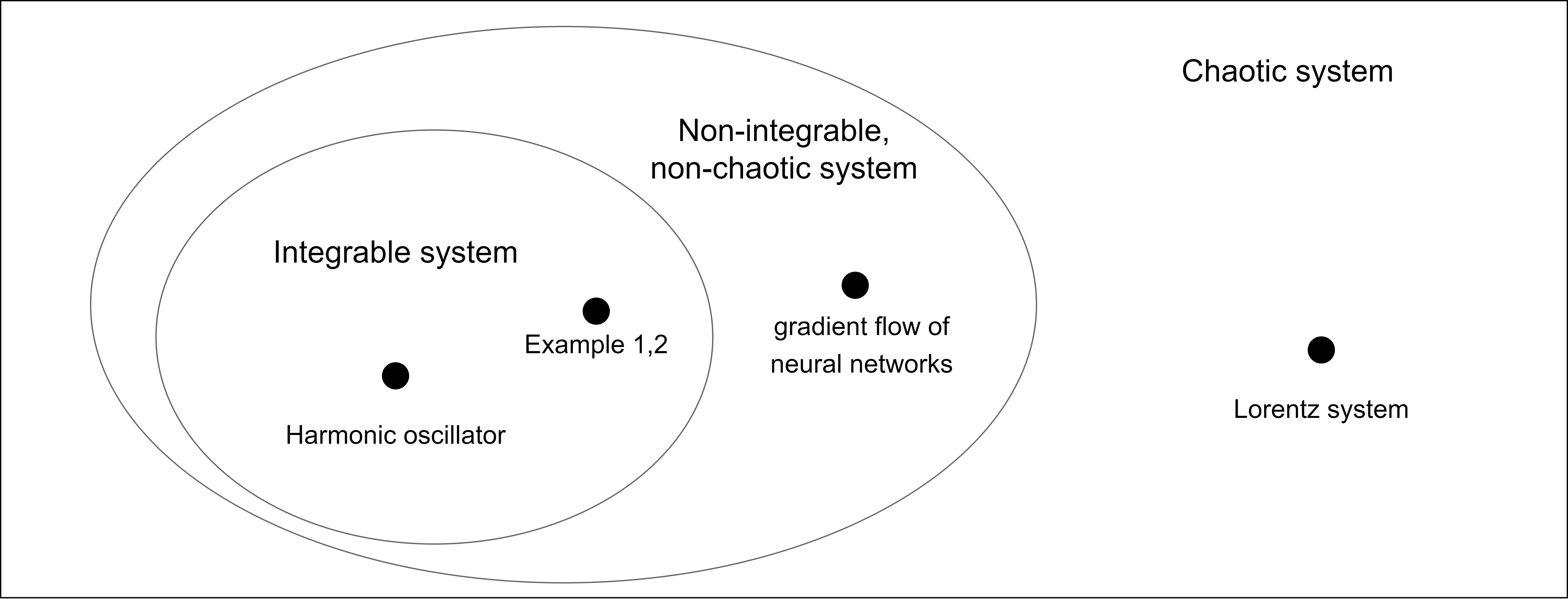
Figure 2: A diagram of various dynamical systems. In this diagram, we denote an integrable system as an integrable system in the meromorphic category.

Nevertheless, it is important to note that non-integrability does not necessarily imply chaos in training neural networks. When the activation function is analytic and the gradient flow possesses a limit point, convergence is guaranteed by Łojasiewicz inequality [4]. Additionally, a wealth of research also supports the convergence of both gradient flow and gradient descent in sufficiently wide neural networks [5, 6, 7, 8]. Thus, we assert that the gradient flow of a neural network is non-integrable and non-chaotic, positioning it between integrable and chaotic systems (Figure 2). Now, we present our contributions as follows.

• We show that under a mind condition (Assumption 1, $\sum_{i}x_{i}\neq 0$), the gradient flow of even a two-layer narrow network is not integrable (Theorem 1).

• In addition, we show that full dynamics of gradient flow cannot be expressed by closed-form (Theorem 2, Corollary 1).

2 Related Work

2.1 Integrability of dynamical systems

The classical three-body problem has played a significant role in the development of integral systems theory. Morales-Ruiz, Ramis, and Simo formulate a theory that describes the meromorphic integrability of Hamiltonian systems using differential Galois theory [9, 10]. Subsequently, [11] and [12] prove the non-integrability of the planar three-body problem.

[13] extend the Morales-Ramis theory to encompass non-Hamiltonian dynamical systems. [14] introduce a novel technique for assessing the integrability of analytic planar vector fields. Leveraging this approach, [15], [16], and [17] examine the non-integrability of Lorentz system. [18] prove the non-integrability of epidemic SEIR models.

2.2 Difficulties in training dynamics of neural networks

There are several studies on the difficulties of training neural networks. In terms of computational complexity, [19] demonstrate that determining the weights of 3-node networks with threshold activations is NP-hard. [20] establishes the NP-hardness of training 3-node networks with sigmoid activations. [21] and [22] prove that training 2-layer ReLU networks is also NP-hard.

In the context of chaotic systems, [23] empirically demonstrate that continuous training dynamics using SGD exhibit locally chaotic behavior. Similarly, [24] empirically show that time-discrete dynamical systems trained by SGD also entail locally chaotic behavior and propose a non-chaotic modified SGD. It is noteworthy that [23] and [24] focus on local chaos as evidenced by the presence of positive local Lyapunov exponents. Specifically, [24] demonstrate that global chaos emerges at the beginning of the training, and diminishes towards the end of training.

3 Preliminaries

In this paper, we assume that the dynamical systems are in $\mathbb{C}$ (the set of complex numbers) for generality. We observe that the actual dynamical systems are projections onto $\mathbb{R}$ (real numbers) of the systems defined in $\mathbb{C}$.

3.1 Integrable dynamical system

Consider the following $n$-dimensional dynamical system with vector field $F(\mathbb{x})$

$$\frac{d\mathbb{x}(t)}{dt}=F(\mathbb{x}),\;\mathbb{x}(t)\in\mathcal{M},\;t\in\mathbb{C},$$ (4)

where $F(\cdot):\mathbb{C}^{n}\to\mathbb{C}^{n}$ is an $n$-dimensional analytic vector-valued function and $\mathcal{M}$ is an $n$-dimensional complex manifold.

An integral curve of the dynamical system represents the trajectory of the system’s state over time, given its initial point.

Definition 1 (integral curve).

We say $\gamma:\mathbb{C}\to\mathcal{M}$ is an integral curve of dynamical system (4) if it follows dynamical system (4) with the initial point $\mathbb{p}\in\mathcal{M}$:

$$\frac{d\gamma(t)}{dt}=F(\gamma(t)),\;\gamma(0)=\mathbb{p},$$ (5)

for $t\in\mathbb{C}$.

A first integral of the dynamical system is a function that remains constant along the trajectories of the system. First integrals are also refereed as conserved quantities or invariants of the system.

Definition 2 (first integral).

We say $\Phi:\mathbb{C}^{n}\to\mathcal{M}$ is a first integral of dynamical system (4) if

$$\frac{d\Phi(\gamma(t))}{dt}=0,\;\forall t\in\mathbb{C},$$ (6)

for any integral curve $\gamma(t)$ of dynamical system (4).

Definition 3 (functionally independent).

Let $f_{1},...,f_{k}:\mathcal{M}\to\mathbb{C}$ be $n$ smooth functions where $\mathcal{M}$ is $n$-dimensional complex manifold. We say $f_{1},...,f_{k}$ are functionally independent if $\nabla f_{1},...,\nabla f_{k}$ are linearly independent, i.e., if the Jacobian has full rank.

If $f_{1},...,f_{k}$ are functionally independent, then their level sets intersect transversely.

Definition 4 (completely integrable).

We say system (4) is completely integrable if it admits $(n-1)$ functionally independent first integrals $\Phi_{1},...,\Phi_{n-1}$.

If system (4) is completely integrable, then its trajectory $\gamma(t)$ is analytically obtained in an explicit way since $\gamma(t)$ is contained in specific one-dimensional manifold $\mathcal{N}$,

$$\gamma(t)\subset\mathcal{N},\;\mathcal{N}=\bigcap_{i=1}^{n-1}\{p\in\mathcal{M}:\Phi_{i}(p)=c_{i},\;c_{i}\in\mathbb{C}\},$$ (7)

and $c_{i}$’s are specified by an initial point $\gamma(0)$.

Definition 5 (B-integrable).

We say system (4) is B-integrable if it admits $(n-k)$ functionally independent first integrals $\Phi_{1},...,\Phi_{n-k}$ and linearly independent $k$ vector fields $X_{1}=F,X_{2},...,X_{k}$ such that

$$[X_{i},X_{j}]=0,\;1\leq i\leq j\leq k\;\text{and}\;X_{i}(\Phi_{j})=0,\;1\leq i\leq k,\;1\leq j\leq n-k,$$ (8)

where $[X_{i},X_{j}](\cdot)=X_{i}(X_{j}(\cdot))-X_{j}(X_{i}(\cdot))$ is the Lie bracket.

The notion of B-integrability was introduced by [25]. If system (4) is B-integrable, $n-k$ functionally independent first integrals $\Phi_{1},...,\Phi_{n-k}$ form a $k$-dimensional level set $\mathcal{N}$ which is $k$-dimensional submanifold $\mathcal{N}=\bigcap_{i=1}^{k}\{p\in\mathcal{M}:\Phi_{i}(p)=c_{i},\;c_{i}\in\mathbb{C}\}\subset\mathcal{M}$. The trajectory $\gamma(t)$ lies on $\mathcal{N}$. Additionally, since $k$ linearly independent and commuting vector fields $X_{1}=F,...,X_{k}$ complete $\mathcal{N}$, for each $p\in\mathcal{N}$ there exists a local coordinate chart $(U,\phi)$ centered at $p$ with $\phi:(x_{1},...,x_{n})\mapsto(s_{1},...,s_{k})$ such that $X_{i}=\frac{\partial}{\partial s_{i}}$ for $i=1,...,k$. Therefore, system (4) is completely integrable in $U\subset\mathcal{N}$ with $(k-1)$ first integrals $\Psi_{2}:=\phi^{-1}(s_{2}),...,\Psi_{k}:=\phi^{-1}(s_{k})$. Hence, if the system is B-integrable, then we can conclude that the system is locally completely integrable.

Definition 6 (meromorphic function).

A function $f:\mathcal{M}\subset\mathbb{C}^{n}\to\mathbb{C}$ is called meromorphic on $\mathcal{M}$ if for every $a\in\mathcal{M}$, there is a neighborhood $U\ni a$ and holomorphic functions $p(z),q(z)$ where $q(z)$ is not identically $0$ on $U$ such that

$$f(z)=\frac{p(z)}{q(z)},\;z\in U\setminus q^{-1}(0).$$ (9)

In other words, a meromorphic function is a function that can be expressed as the quotient of holomorphic functions.

Definition 7 (integrable in the meromorphic category).

If system (4) is completely integrable and the vector field $X(t)$ and $(n-1)$ functionally independent first integrals are meromorphic, then we say the system is completely integrable in the meromorphic category.
If system (4) is B-integrable and $(n-k)$ functionally independent first integrals and $k$ commuting vector fields are meromorphic, we say the system is B-integrable in the meromorphic category.

3.1.1 Examples of dynamical systems

We present some examples of integrable dynamical systems.

Example 1.

Let $\mathcal{M}=\mathbb{C}^{2}$. Consider the $2$-dimensional dynamical system with the vector field $F(\mathbb{x})=(-y,x),\;\mathbb{x}=(x,y)\in\mathbb{C}^{2}:$

$$\frac{d\mathbb{x}(t)}{dt}=\begin{bmatrix}x^{\prime}\\ y^{\prime}\end{bmatrix}=\begin{bmatrix}-y\\ x\end{bmatrix}.$$ (10)

Then the system is completely integrable in the meromorphic category since it has a meromorphic first integral $\Phi_{1}(x,y)=x^{2}+y^{2}$. Hence, the trajectory of the system has an explicit form of $\gamma(t)=(x_{0}\cos(t)-y_{0}\sin(t),x_{0}\sin(t)+y_{0}\cos(t))$ with the initial point $\gamma(0)=(x_{0},y_{0})\in\mathbb{C}^{2}$.

Example 2.

Let $\mathcal{M}=\mathbb{C}^{2}$. Consider the $2$-dimensional dynamical system with the vector field $F(\mathbb{x})=(x,y),\;\mathbb{x}=(x,y)\in\mathbb{C}^{2}:$

$$\frac{d\mathbb{x}(t)}{dt}=\begin{bmatrix}x^{\prime}\\ y^{\prime}\end{bmatrix}=\begin{bmatrix}x\\ y\end{bmatrix}.$$ (11)

Then the system is completely integrable in the meromorphic category since it has a meromorphic first integral $\Phi_{1}(x,y)=\frac{y}{x}.$ Hence, the trajectory of the system has an explicit form of $\gamma(t)=(x_{0}e^{t},y_{0}e^{t})$ with the initial point $\gamma(0)=(x_{0},y_{0})\in\mathbb{C}^{2}$.

Example 3 (simple harmonic oscillator).

We consider a motion of a simple harmonic oscillator.

$$\frac{d^{2}x(t)}{dt^{2}}+\omega_{0}^{2}x(t)=0,$$ (12)

where $x(t)$ is the displacement of the oscillator and $\omega_{0}\neq 0$ is the angular frequency of the oscillator. We can restate equation (12) as a dynamical system.

$$\frac{d\mathbb{x}(t)}{dt}=\begin{bmatrix}x^{\prime}\\ y^{\prime}\end{bmatrix}=\begin{bmatrix}y\\ -\omega_{0}^{2}x\end{bmatrix},$$ (13)

where $\mathbb{x}(t)=(x(t),y(t))$, $y(t):=x^{\prime}(t)$ is the velocity of the oscillator. The trajectory of the system has an explicit form of $\gamma(t)=(\frac{v_{0}}{\omega_{0}}\sin(\omega_{0}t)+x_{0}\cos(\omega_{0}t),v_{0}\cos(\omega_{0}t)-\omega_{0}x_{0}\sin(\omega_{0}t))$ with the initial condition $x(0)=x_{0},x^{\prime}(0)=v_{0}$. Moreover, the system is completely integrable in the meromorphic category since it has a meromorphic first integral $\Phi(x,y)=\omega_{0}^{2}x^{2}+y^{2}$.

Next, we present the famous Lorentz system [27].

Example 4 (Lorentz system).

Let $\mathcal{M}=\mathbb{C}^{3}$. Consider the Lorentz system

$$x^{\prime}(t) =-\sigma x+\sigma y$$ (14)

$$y^{\prime}(t) =rx-y-xz$$ (15)

$$z^{\prime}(t) =xy-\beta z,$$ (16)

where $\sigma,r,\beta\in\mathbb{C}$.
If $\sigma=0$, [15] show that the Lorentz system is completely integrable with two first integrals. [16] show that if $\sigma\beta\neq 0$, the Lorentz system is not completely integrable in the meromorphic category. Moreover if $\frac{2\sqrt{(\sigma+1)^{2}+4\sigma(r-1)}}{|\beta|}$ is not odd integer, the Lorentz system is not B-integrable in the meromorphic category. Moreover, the Lorentz system is chaotic for specific configurations of $(\sigma,r,\beta)$ [28, 29, 30].

3.2 Differential Galois theory

Differential Galois theory plays an important role in demonstrating the impossibility of representing solutions of linear ODEs in closed-form. In this section, we present the formal definition of Liouvillian functions. We defer a brief introduction to differential Galois theory to appendix C.

Definition 8 (Liouvillian extension, Liouvillian function).

Let $K\subset L$ be a differential field extension. We say $l\in L$ is Liouvillian over $K$ if $l$ is either algebraic, primitive, or exponential over $K$. Similarly, a differential field extension $K\subset L$ is Liouvillian if there exists a finite sequence of intermediate differential field extensions

$$K=K_{0}\subset K_{1}\subset...\subset K_{n}=L,$$ (17)

such that $K_{i+1}=K_{i}(l_{i})$ and $l_{i}$ is Liouvillian over $K_{i}\;$ for $1\leq i\leq n$. $l$ is called Liouvillian over $K$ if $K\subset K(l)$ is a Liouvillian extension.
If $l$ is Liouvillian over $\mathbb{C}(x)$, we simply call $l$ be a Liouvillian function.

Thus, if $l$ is Liouvillian, $l$ is representable by a finite number of additions, multiplications, $n$-th roots, exponentials, and anti-derivatives of algebraic functions.

Next, we present the useful lemma to determine the solvability of specific form of the second order ODE.

Lemma 1.

Consider the following second order ODE

$$L(y) =y(t)^{\prime\prime}-ry(t),$$

$$r =a_{2}t^{2}+a_{1}t+a_{0}+\frac{a_{-1}}{t+d}+\frac{b}{(t+d)^{2}},$$

where $a_{2},a_{1},a_{0},a_{-1},b,d\in\mathbb{C}$. If $a_{2},b\neq 0$ and $-2+\sqrt{1+4b}$ is not a nonnegative integer, then $L(y)$ has no Liouvillian solution and its differential Galois group is $Gal(L(y))=SL_{2}(\mathbb{C})$.

Proof.

The proof is presented in section D.1. ∎

3.3 Morales-Ramis theory on integrability of dynamical systems

Now we present the Morales-Ramis theory, an application of differential Galois theory to dynamical systems, which describes the integrability of these systems.

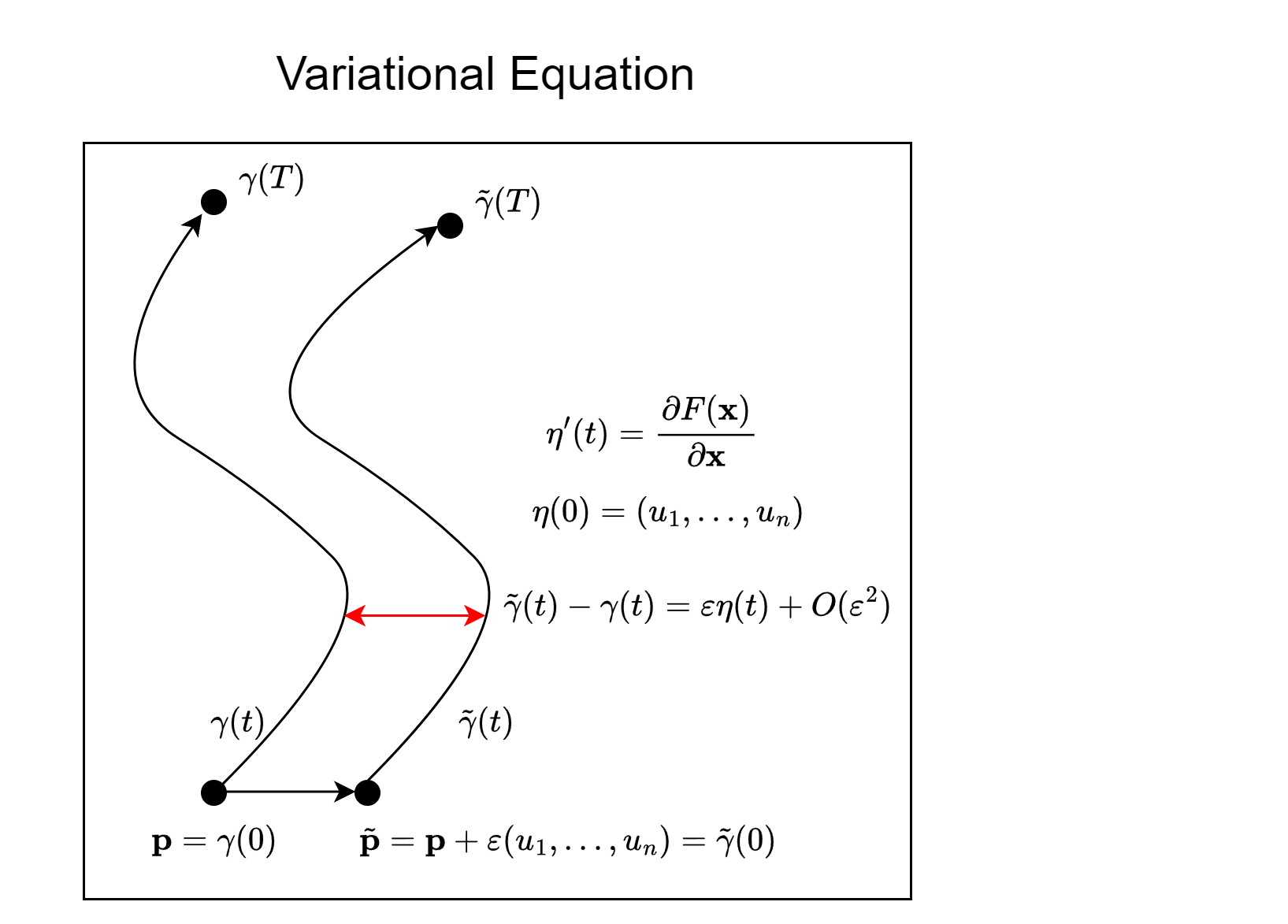
Figure 3: An illustration of variational equations of dynamical system $\frac{d\mathbb{x}(t)}{dt}=F(\mathbb{x})$. For the integral curve $\gamma(t)$ with the initial point $\mathbb{p}$, $\tilde{\gamma}(t)$ denotes the perturbed curve with the perturbed initial point $\tilde{\mathbb{p}}$. Let $\eta(t)$ follow variational equation (18) with the initial condition $\eta(0)=(u_{1},...,u_{n})$. Then $\varepsilon\eta(t)$ is the first-order approximation (in terms of $\varepsilon$) of the perturbations ($\tilde{\gamma}(t)-\gamma(t)$) of the integral curve $\gamma(t)$.

Definition 9 (variational equation).

Consider dynamical system (4). Let $\gamma(t)$ be an integral curve of the system. Then we consider the following linear differential equation for $\eta(t):\mathbb{C}\to\mathbb{C}^{n}$:

$$\frac{d\eta(t)}{dt}=A(t)\eta(t),\;A(t)=\frac{\partial F(\mathbb{x}(t))}{\partial\mathbb{x}}\in\mathbb{C}^{n\times n},\;\eta(t)\in T\mathcal{M},$$ (18)

where $T\mathcal{M}$ is the tangent bundle. Equation (18) is called the variational equation ($VE_{\gamma(t)}$) along $\gamma(t)$.

The variational equation describes how perturbation evolves along the trajectory $\gamma(t)$. Please refer to Figure 3 for an illustration of variational equations.

Remark 1.

We can understand variational equations as follows. Let $\gamma(t)$ be an integral curve of the dynamical system (4) with the initial point $\mathbf{p}$. Let $\tilde{\mathbf{p}}=\mathbf{p}+\varepsilon(u_{1},...,u_{n})$ be a perturbed point of $\mathbf{p}$ with a small perturbation $\varepsilon$, and let $\tilde{\gamma}$ be the integral curve with initial point $\tilde{\mathbf{p}}$. Then the difference $\tilde{\gamma}(t)-\gamma(t)$ follows the equation

$$\tilde{\gamma}(t)-\gamma(t)=\varepsilon\eta(t)+O(\varepsilon^{2}),\;\text{as}\;\varepsilon\to 0,$$ (19)

where $\eta(t)$ satisfies

$$\eta^{\prime}(t) =\lim_{\varepsilon\to 0}\frac{F(\tilde{\gamma}(t))-F(\gamma(t))}{\varepsilon}$$

$$=\lim_{\varepsilon\to 0}\frac{F(\gamma(t)+\varepsilon\eta(t)+O(\varepsilon^{2}))-F(\gamma(t))}{\varepsilon}=\frac{\partial F(\mathbb{x})}{\partial\mathbb{x}}\eta(t),$$

with the initial condition $\eta(0)=(u_{1},...,u_{n})$. Therefore $\eta(t)$ is the solution of the variational equation. Hence, we can conclude that the variational equation describes the first-order approximation (in terms of $\varepsilon$) of the perturbation of the integral curve $\gamma(t)$.

Now, we present an important statement to demonstrate the non-integrability of the dynamical systems.

Lemma 2 ([13]).

Suppose a dynamical system is B-integrable in the meromorphic category in a neighborhood of its integral curve $\gamma(t)$. Then the identity component $Gal^{0}(VE_{\gamma(t)})$ of the differential Galois group $Gal(VE_{\gamma})$ of the variational equations $VE_{\gamma(t)}$ is abelian.

For a given linear differential equation $L(y)$, the differential Galois group $Gal(L(y))$ is the group of automorphisms that map the solutions of $L(y)$ to themselves. We can demonstrate the non-integrability of the system by showing that $Gal^{0}(VE_{\gamma(t)})$ is not abelian. The integrabililty of the dynamical system is closely related to the differential Galois group. lemma 2 is useful for determining the integrability of the dynamical system. We will show the non-integrability of the gradient flow of neural networks using lemma 2.

We provide a brief history of Morales-Ramis theory. Morales, Ramis and Simo demonstrate the obstruction to meromorphic integrability of Hamiltonian systems in terms of differential Galois theory [9, 10]. [13] further extend this result to the general non-Hamiltonian dynamical system.

4 Non-integrability of gradient flow

In this section, we present our main statement that the gradient flow of a two-layer narrow network is not B-integrable in the meromorphic category. First, we assume that the activation function $\sigma(x)$ satisfies the following assumption:

Assumption 1.

Suppose that the activation function $\sigma(x)$ is analytic and $\sigma^{\prime}(\hat{b})=0$ at some $\hat{b}\in\mathbb{R}$ with $\sigma(\hat{b}),\sigma^{\prime\prime}(\hat{b})\neq 0$.

Roughly speaking, $\sigma(x)$ locally exhibits a non-zero U-like shape around around $x=\hat{b}$. Modern smooth activation functions feature a smoother ReLU-like profile ($\sigma(x)\to 0$ as $x\to-\infty$ and $\sigma(x)\to x$ as $x\to\infty$). Consequently, most smooth activation functions satisfy Assumption 1. Notably, a variety of activation functions such as SiLU [31], SoftPlus, GELU [32], Swish [33], and Mish [34] satisfy Assumption 1.

Now, we restate the following two-layer narrow network with $\ell^{2}$ loss and four parameters $W=(w_{1},b_{1},w_{2},b_{2})\in\mathbb{R}^{4}$ with the dataset $x_{1},...,x_{N},y_{1},...,y_{N}\in\mathbb{R}$.

$$F(x,W) =w_{2}\sigma(w_{1}x+b_{1})+b_{2},$$

$$\mathcal{R}(W) =\frac{1}{2}\sum_{i=1}^{N}(F(x_{i},W)-y_{i})^{2}=\frac{1}{2}\sum_{i=1}^{N}(w_{2}\sigma(w_{1}x_{i}+b_{1})+b_{2}-y_{i})^{2},$$

where $N$ denotes the number of samples. $F(x,W)$ denote the output of the network with input $x$ and the set of parameters $W$, and $\mathcal{R}(W)$ denote the $\ell^{2}$ loss. Then, we have the following dynamical system of the gradient flow:

$$W^{\prime}(t)=-\frac{\partial\mathcal{R}}{\partial W}.$$

The component-wise expressions of the gradient flow are as follows:

$$w_{1}^{\prime}(t) =-\frac{\partial\mathcal{R}}{\partial w_{1}}=-\sum_{i=1}^{N}(w_{2}\sigma(w_{1}x_{i}+b_{1})+b_{2}-y_{i})(w_{2}\sigma^{\prime}(w_{1}x_{i}+b_{1}))x_{i},$$ (20)

$$b_{1}^{\prime}(t) =-\frac{\partial\mathcal{R}}{\partial b_{1}}=-\sum_{i=1}^{N}(w_{2}\sigma(w_{1}x_{i}+b_{1})+b_{2}-y_{i})(w_{2}\sigma^{\prime}(w_{1}x_{i}+b_{1})),$$ (21)

$$w_{2}^{\prime}(t) =-\frac{\partial\mathcal{R}}{\partial w_{2}}=-\sum_{i=1}^{N}(w_{2}\sigma(w_{1}x_{i}+b_{1})+b_{2}-y_{i})(\sigma(w_{1}x_{i}+b_{1})),$$ (22)

$$b_{2}^{\prime}(t) =-\frac{\partial\mathcal{R}}{\partial b_{2}}=-\sum_{i=1}^{N}(w_{2}\sigma(w_{1}x_{i}+b_{1})+b_{2}-y_{i}).$$ (23)

Now we formally present our main theorem.

Theorem 1.

Suppose the activation function $\sigma$ satisfies Assumption 1 and
$\sum_{i=1}^{N}x_{i}\neq 0$. Then the dynamical system of the gradient flow (20)-(23) is not B-integrable in the meromorphic category.

Remark 2.

We clarify that throughout the proof, we consider all numbers as belonging to $\mathbb{C}$ although they are actually real numbers as mentioned in Section 3.

Proof.

Before beginning the proof, we will briefly outline our proof strategy. First, we find the integral curve $\gamma(t)$ of the gradient flow (lemma 3). Next, we obtain the variational equation $\eta(t)$ along the integral curve $\gamma(t)$ (lemma 4)). Then we reduce the variational equation $\eta(t)$ into a second-order ODE (lemmas 5, 6, and 7). Using lemma 1, we verify that the variation equation has no Liouvillian solution and that its differential Galois group is not abelian. Finally using lemma 2, we conclude that gradient flow is not B-integrable in the meromorphic category. The proofs of lemmas 3, 4, 5, 6, and 7 are presented in appendix B.

Now, we begin the proof by defining the following five quantities.

$$\mkern 1.5mu\overline{\mkern-1.5mux\mkern-1.5mu}\mkern 1.5mu =\frac{1}{N}\sum_{i=1}^{N}x_{i},\;\mkern 1.5mu\overline{\mkern-1.5muy\mkern-1.5mu}\mkern 1.5mu=\frac{1}{N}\sum_{i=1}^{N}y_{i},\;\mkern 1.5mu\overline{\mkern-1.5mux^{2}\mkern-1.5mu}\mkern 1.5mu=\frac{1}{N}\sum_{i=1}^{N}x_{i}^{2},$$

$$\mkern 1.5mu\overline{\mkern-1.5muxy\mkern-1.5mu}\mkern 1.5mu =\frac{1}{N}\sum_{i=1}^{N}x_{i}y_{i},\;\mkern 1.5mu\overline{\mkern-1.5mux^{2}y\mkern-1.5mu}\mkern 1.5mu=\frac{1}{N}\sum_{i=1}^{N}x_{i}^{2}y_{i}.$$

Next, we find the following integral curve $\gamma(t)$ starting from an initial point $\gamma(0)=(0,\hat{b},a\sigma(\hat{b}),\hat{b}_{2})$:

$$\gamma(t)=(w_{1}(t),b_{1}(t),w_{2}(t),b_{2}(t))=(0,\hat{b},a\sigma(\hat{b})e^{-\omega t},ae^{-\omega t}+\mkern 1.5mu\overline{\mkern-1.5muy\mkern-1.5mu}\mkern 1.5mu),$$ (24)

where $\omega=N(\sigma(\hat{b})^{2}+1),a=\hat{b}_{2}-\mkern 1.5mu\overline{\mkern-1.5muy\mkern-1.5mu}\mkern 1.5mu\neq 0$, and $\hat{b}_{2}\in\mathbb{R}$ can be arbitrary and determined later.

Lemma 3.

$\gamma(t)$ is an integral curve of the gradient flow (20)-(23).

To exploit Lemma 2, we attain the variational equation along the integral curve $\gamma(t)$. We have the following variational equation $\eta(t)$ along $\gamma(t)$:

$$\frac{d\eta(t)}{dt}=\frac{\partial}{\partial W}(-\frac{\partial\mathcal{R}}{\partial W})\eta(t)=\frac{\partial}{\partial W}\left(\begin{bmatrix}{w^{\prime}_{1}}(t)\\ {b^{\prime}_{1}}(t)\\ {w^{\prime}_{2}}(t)\\ {b^{\prime}_{2}}(t)\end{bmatrix}\right)\begin{bmatrix}\epsilon_{w_{1}}(t)\\ \epsilon_{b_{1}}(t)\\ \epsilon_{w_{2}}(t)\\ \epsilon_{b_{2}}(t)\end{bmatrix},$$

$$\eta^{\prime}(t)=\begin{bmatrix}\epsilon_{w_{1}}^{\prime}(t)\\ \epsilon_{b_{1}}^{\prime}(t)\\ \epsilon_{w_{2}}^{\prime}(t)\\ \epsilon_{b_{2}}^{\prime}(t)\end{bmatrix}=\begin{bmatrix}\frac{\partial w_{1}^{\prime}(t)}{\partial w_{1}}&\frac{\partial w_{1}^{\prime}(t)}{\partial b_{1}}&\frac{\partial w_{1}^{\prime}(t)}{\partial w_{2}}&\frac{\partial w_{1}^{\prime}(t)}{\partial b_{2}}\\ \frac{\partial b_{1}^{\prime}(t)}{\partial w_{1}}&\frac{\partial b_{1}^{\prime}(t)}{\partial b_{1}}&\frac{\partial b_{1}^{\prime}(t)}{\partial w_{2}}&\frac{\partial b_{1}^{\prime}(t)}{\partial b_{2}}\\ \frac{\partial w_{2}^{\prime}(t)}{\partial w_{1}}&\frac{\partial w_{2}^{\prime}(t)}{\partial b_{1}}&\frac{\partial w_{2}^{\prime}(t)}{\partial w_{2}}&\frac{\partial w_{2}^{\prime}(t)}{\partial b_{2}}\\ \frac{\partial b_{2}^{\prime}(t)}{\partial w_{1}}&\frac{\partial b_{2}^{\prime}(t)}{\partial b_{1}}&\frac{\partial b_{2}^{\prime}(t)}{\partial w_{2}}&\frac{\partial b_{2}^{\prime}(t)}{\partial b_{2}}\end{bmatrix}\begin{bmatrix}\epsilon_{w_{1}}(t)\\ \epsilon_{b_{1}}(t)\\ \epsilon_{w_{2}}(t)\\ \epsilon_{b_{2}}(t)\end{bmatrix}.$$ (25)

for $\eta(t)=(\epsilon_{w_{1}}(t),\epsilon_{b_{1}}(t),\epsilon_{w_{2}}(t),\epsilon_{b_{2}}(t))^{T}\in\mathbb{C}^{4}$.

Lemma 4.

The variational equation $\eta(t)$ along the integral curve $\gamma(t)$ has the following forms.

$$\epsilon_{w_{1}}^{\prime}(t) =\begin{bmatrix}-\sum_{i=1}^{N}(a\frac{\omega}{N}e^{-\omega t}+\mkern 1.5mu\overline{\mkern-1.5muy\mkern-1.5mu}\mkern 1.5mu-y_{i})(a\sigma(\hat{b})e^{-\omega t}\sigma^{\prime\prime}(\hat{b})x_{i}^{2})\\ -\sum_{i=1}^{N}(a\frac{\omega}{N}e^{-\omega t}+\mkern 1.5mu\overline{\mkern-1.5muy\mkern-1.5mu}\mkern 1.5mu-y_{i})(a\sigma(\hat{b})e^{-\omega t}\sigma^{\prime\prime}(\hat{b})x_{i})\\ 0\\ 0\end{bmatrix}^{T}\begin{bmatrix}\epsilon_{w_{1}}(t)\\ \epsilon_{b_{1}}(t)\\ \epsilon_{w_{2}}(t)\\ \epsilon_{b_{2}}(t)\end{bmatrix},$$ (26)

$$\epsilon_{b_{1}}^{\prime}(t) =\begin{bmatrix}-\sum_{i=1}^{N}(a\frac{\omega}{N}e^{-\omega t}+\mkern 1.5mu\overline{\mkern-1.5muy\mkern-1.5mu}\mkern 1.5mu-y_{i})(a\sigma(\hat{b})e^{-\omega t}\sigma^{\prime\prime}(\hat{b})x_{i})\\ -\sum_{i=1}^{N}(a\frac{\omega}{N}e^{-\omega t}+\mkern 1.5mu\overline{\mkern-1.5muy\mkern-1.5mu}\mkern 1.5mu-y_{i})(a\sigma(\hat{b})e^{-\omega t}\sigma^{\prime\prime}(\hat{b}))\\ 0\\ 0\end{bmatrix}^{T}\begin{bmatrix}\epsilon_{w_{1}}(t)\\ \epsilon_{b_{1}}(t)\\ \epsilon_{w_{2}}(t)\\ \epsilon_{b_{2}}(t)\end{bmatrix},$$ (27)

$$\epsilon_{w_{2}}^{\prime}(t) =\begin{bmatrix}0\\ 0\\ -\sum_{i=1}^{N}\sigma(\hat{b})^{2}\\ -\sum_{i=1}^{N}\sigma(\hat{b})\end{bmatrix}^{T}\begin{bmatrix}\epsilon_{w_{1}}(t)\\ \epsilon_{b_{1}}(t)\\ \epsilon_{w_{2}}(t)\\ \epsilon_{b_{2}}(t)\end{bmatrix},$$ (28)

$$\epsilon_{b_{2}}^{\prime}(t) =\begin{bmatrix}0\\ 0\\ -\sum_{i=1}^{N}\sigma(\hat{b})\\ -\sum_{i=1}^{N}1\end{bmatrix}^{T}\begin{bmatrix}\epsilon_{w_{1}}(t)\\ \epsilon_{b_{1}}(t)\\ \epsilon_{w_{2}}(t)\\ \epsilon_{b_{2}}(t)\end{bmatrix}.$$ (29)

Therefore, we can separate the case of $\epsilon_{w_{1}}(t),\epsilon_{b_{1}}(t)$ and the case of $\epsilon_{w_{2}}(t),\epsilon_{b_{2}}(t)$.

Lemma 5.

The differential Galois groups for $\epsilon_{w_{2}}(t)$ and $\epsilon_{b_{2}}(t)$ are $\mathbb{C}^{\ast}$, hence they are abelian.

Therefore, we only need to care the case of $\epsilon_{w_{1}}(t),\epsilon_{b_{1}}(t)$.

Lemma 6.

Let $\tau:=e^{-\omega t}$ and $g_{w_{1}}(\tau):=\epsilon_{w_{1}}(t)$. THen we have the following second-order ODE for $g_{w_{1}}(\tau)$:

$$g_{w_{1}}^{\prime\prime}(\tau)=P_{1}(\tau)g_{w_{1}}^{\prime}(\tau)+P_{2}(\tau)g_{w_{1}}(\tau),$$ (30)

where

$$P_{1}(\tau)=A_{1,1}\tau+B_{1,1}+(A_{1,2}\tau+B_{1,2})^{-1}\big{(}A_{1,2}+(A_{1,2}\tau+B_{1,2})(A_{2,2}\tau)\big{)},$$

$$P_{2}(\tau)=A_{1,1}+(A_{1,2}\tau+B_{1,2})(A_{1,2}\tau+B_{1,2})$$

$$-(A_{1,2}\tau+B_{1,2})^{-1}(A_{1,1}\tau+B_{1,1})\big{(}A_{1,2}+(A_{1,2}\tau+B_{1,2})(A_{2,2}\tau)\big{)}.$$

Lemma 7.

Define the transformation $T$ as
$T(f(\tau))$ $=f(\tau)e^{\frac{\int P_{1}(\tau)d\tau}{2}}$. Let $y(\tau)=T(g_{w_{1}}(\tau))$. Then we have

$$y^{\prime\prime}(\tau) =\big{(}r_{2}\tau^{2}+r_{1}\tau+r_{0}+\frac{r_{-1}}{\tau+A_{1,2}^{-1}B_{1,2}}+\frac{r_{-2}}{(\tau+A_{1,2}^{-1}B_{1,2})^{2}}\big{)}y(\tau),$$ (31)

where

$$r_{2} =(\frac{1}{4}A_{1,1}^{2}+A_{1,2}^{2}+\frac{1}{4}A_{2,2}-\frac{1}{2}A_{1,1}A_{2,2}),$$

$$r_{1} =\frac{1}{2}A_{1,1}B_{1,1}+2A_{1,2}B_{1,2}-\frac{1}{2}B_{1,1}A_{2,2}-1,$$

$$r_{0} =\frac{1}{4}B_{1,1}^{2}+B_{1,2}^{2},$$

$$r_{-1} =\frac{1}{2}A_{1,2}^{-1}B_{1,2}(A_{1,1}-A_{2,2})-\frac{1}{2}B_{1,1},$$

$$r_{-2} =-\frac{1}{4}.$$

and

$$A_{1,1}=a^{2}\sigma(\hat{b})\sigma^{\prime\prime}(\hat{b})\mkern 1.5mu\overline{\mkern-1.5mux^{2}\mkern-1.5mu}\mkern 1.5mu,$$ (32)

$$B_{1,1}=\frac{1}{\omega}Na\sigma(\hat{b})\sigma^{\prime\prime}(\hat{b})(\mkern 1.5mu\overline{\mkern-1.5mux^{2}\mkern-1.5mu}\mkern 1.5mu\mkern 1.5mu\overline{\mkern-1.5muy\mkern-1.5mu}\mkern 1.5mu-\mkern 1.5mu\overline{\mkern-1.5mux^{2}y\mkern-1.5mu}\mkern 1.5mu),$$ (33)

$$A_{1,2}=A_{2,1}=a^{2}\sigma(\hat{b})\sigma^{\prime\prime}(\hat{b})\mkern 1.5mu\overline{\mkern-1.5mux\mkern-1.5mu}\mkern 1.5mu,$$ (34)

$$B_{1,2}=B_{2,1}=\frac{1}{\omega}Na\sigma(\hat{b})\sigma^{\prime\prime}(\hat{b})(\mkern 1.5mu\overline{\mkern-1.5mux\mkern-1.5mu}\mkern 1.5mu\cdot\mkern 1.5mu\overline{\mkern-1.5muy\mkern-1.5mu}\mkern 1.5mu-\mkern 1.5mu\overline{\mkern-1.5muxy\mkern-1.5mu}\mkern 1.5mu),$$ (35)

$$A_{2,2}=a^{2}\sigma(\hat{b})\sigma^{\prime\prime}(\hat{b}),$$ (36)

$$B_{2,2}=0.$$ (37)

Note that since $\mkern 1.5mu\overline{\mkern-1.5mux\mkern-1.5mu}\mkern 1.5mu\neq 0$, we have $A_{1,2}\neq 0$.

Hence, by lemmas 5 and 6, we need to explore the solvability of $y(\tau)$ in eq. 31 to determine the solvability of $\epsilon_{w_{1}}(t)$. Now, we apply Lemma 1 to determine the solvability of ODE (31). By lemma 1, if $r_{2},r_{-2}\neq 0$ and $-2+\sqrt{1+4r_{-2}}$ is not a nonnegative integer, ODE eq. 31 has no Liouvillian solution. Since $-2+\sqrt{1+4r_{-2}}=-2+\sqrt{1+4\times(-\frac{1}{4})}=-2\not\in\mathbb{N}_{\geq 0}$, we only need to see whether $r_{2}\neq 0$. By plugging (32)-(37) into $r_{2}$, we have

$$r_{2}=a^{4}\sigma(\hat{b})^{2}\sigma^{\prime\prime}(\hat{b})^{2}(\mkern 1.5mu\overline{\mkern-1.5mux^{2}\mkern-1.5mu}\mkern 1.5mu)^{2}+4a^{4}\sigma(\hat{b})^{2}\sigma^{\prime\prime}(\hat{b})^{2}(\mkern 1.5mu\overline{\mkern-1.5mux\mkern-1.5mu}\mkern 1.5mu)^{2}+a^{2}\sigma(\hat{b})\sigma^{\prime\prime}(\hat{b})-2a^{4}\sigma(\hat{b})^{2}\sigma^{\prime\prime}(\hat{b})^{2}\mkern 1.5mu\overline{\mkern-1.5mux^{2}\mkern-1.5mu}\mkern 1.5mu\mkern 1.5mu\overline{\mkern-1.5mux\mkern-1.5mu}\mkern 1.5mu.$$

Hence $r_{2}=0$ if and only if

$$(\mkern 1.5mu\overline{\mkern-1.5mux^{2}\mkern-1.5mu}\mkern 1.5mu)^{2}+4(\mkern 1.5mu\overline{\mkern-1.5mux\mkern-1.5mu}\mkern 1.5mu)^{2}-2\mkern 1.5mu\overline{\mkern-1.5mux^{2}\mkern-1.5mu}\mkern 1.5mu\mkern 1.5mu\overline{\mkern-1.5mux\mkern-1.5mu}\mkern 1.5mu+\frac{1}{a^{2}\sigma(\hat{b})\sigma^{\prime\prime}(\hat{b})}$$

$$= (\mkern 1.5mu\overline{\mkern-1.5mux^{2}\mkern-1.5mu}\mkern 1.5mu)^{2}+4(\mkern 1.5mu\overline{\mkern-1.5mux\mkern-1.5mu}\mkern 1.5mu)^{2}-2\mkern 1.5mu\overline{\mkern-1.5mux^{2}\mkern-1.5mu}\mkern 1.5mu\mkern 1.5mu\overline{\mkern-1.5mux\mkern-1.5mu}\mkern 1.5mu+\frac{1}{(\hat{b}_{2}-\mkern 1.5mu\overline{\mkern-1.5muy\mkern-1.5mu}\mkern 1.5mu)^{2}\sigma(\hat{b})\sigma^{\prime\prime}(\hat{b})}=0,$$

Since $\hat{b}_{2}\in\mathbb{R}$ is arbitrary, we can always choose $\hat{b}_{2}\neq\mkern 1.5mu\overline{\mkern-1.5muy\mkern-1.5mu}\mkern 1.5mu$ such that $r_{2}\neq 0$. Therefore, ODE (31) has no Liouvillian solution, and its differential Galois group is $SL_{2}(\mathbb{C})$. Hence $\epsilon_{w_{1}}(t),\epsilon_{b_{1}}(t)$ also has no Liouvillian solution, and its differential Galois group is also $SL_{2}(\mathbb{C})$ that is not solvable (also not abelian). Since the differential Galois group of the variational equation is not abelian, the gradient flow is not B-integrable in the meromorphic category by Lemma 2. This completes the proof. ∎

5 Absence of the closed-form description of the gradient flow

In this section, we show demonstrate the unsolvability of the variational equation implies the absence of a closed-form description for the dynamical system.

Theorem 2.

Consider the following $n$-dimensional system

$$\frac{d\mathbb{x}(t)}{dt}=F(\mathbb{x}),\;\mathbb{x}(t)\in\mathcal{M},\;t\in\mathbb{C},$$ (38)

where $F(\mathbb{x})$ is an $n$-dimensional vector-valued function and $\mathcal{M}$ is an $n$-dimensional complex manifold. Let $\gamma(t)$ be an integral flow of system (38) with the initial point $\mathbf{p}_{1}\in\mathbb{C}^{n}$. Suppose that the variational equation of $\gamma(t)$ has no Liouvillian solution. Then there is no Liouvillain function $\Gamma(\cdot):\mathbb{C}\times\mathbb{C}^{n}\to\mathbb{C}^{n}$ which describes the full dynamics (38).

Proof.

Suppose that such Liouvillian $\Gamma(\cdot)$ exists. That is, $\Gamma(t,\mathbf{p})$ is the trajectory with the initial point $\mathbf{p}\in\mathbb{C}$ ( $\Gamma(t,\mathbf{p})$ is an integral curve starting from $\mathbf{p}$ for some $\mathbb{p}\in\mathbb{C}^{n}$). Let $\eta(t)=\frac{\partial}{\partial\mathbb{x}}\Gamma(t,\mathbb{p}_{1})\mathbb{u}\in\mathbb{C}^{n}$ for some $\mathbb{u}=(u_{1},...,u_{n})\in\mathbb{C}^{n}$. Since $\Gamma(\cdot)$ is Liouvillian, $\frac{\partial}{\partial\mathbb{x}}\Gamma(t,\mathbb{p}_{1})$ is also Liouvillian. Since $\Gamma(0,\mathbb{x})=\mathbb{x}$, we have $\frac{\partial}{\partial\mathbb{x}}\Gamma(0,\mathbb{x})=I_{n}$ where $\mathbb{x}\in\mathbb{C}^{n}$, and $I_{n}$ is the $n\times n$ identity matrix. Hence,

$$\eta(0)=\mathbb{u},\;\eta^{\prime}(t)=\frac{\partial}{\partial t}\frac{\partial}{\partial\mathbb{x}}\Gamma(t,\mathbb{p}_{1})\mathbb{u}=\frac{\partial}{\partial\mathbb{x}}\frac{\partial}{\partial t}\Gamma(t,\mathbb{p}_{1})\mathbb{u}=\frac{\partial}{\partial\mathbb{x}}\big{(}F(\Gamma(t,\mathbb{p}))\big{)}\mathbb{u}$$

$$=\frac{dF}{d\mathbb{x}}(\Gamma(t,\mathbb{p}_{1}))\frac{\partial\Gamma}{\partial\mathbb{x}}(t,\mathbb{p}_{1})\mathbb{u}=\frac{dF}{d\mathbb{x}}(\Gamma(t,\mathbb{p}_{1}))\eta(t).$$

Therefore, $\eta(t)$ follows the variational equation along $\gamma(t)$ with the initial condition $\eta(0)=\mathbb{u}$. However, since the variational equation along $\gamma(t)$ has no Liouvillian solution, this contradicts the fact that $\frac{\partial}{\partial\mathbb{x}}\Gamma(t,\mathbb{p}_{1})$ is Liouvillian. ∎

Using Theorem 1 and Theorem 2, we can demonstrate that there is no closed-form description of full training dynamics (20)-(23).

Corollary 1.

There is no Liouvillian function $\Gamma(\cdot):\mathbb{C}\times\mathbb{C}^{4}\to\mathbb{C}^{4}$ which describes full dynamics (20)-(23).

6 Discussion

We demonstrate the absence of a closed-form description for the gradient flow in two-layer narrow networks. A natural question arises: Is it possible to extend this result to general neural networks? As the number of parameters increases, the dynamics likely become more complex, leading us to expect that the gradient flow in general networks is also sufficiently complex. However, providing a strict proof is challenging due to the difficulties associated with determining the differential Galois group for general linear differential equations. For second-order and third-order cases, there are algorithms [35, 36] to obtain the differential Galois group. Nevertheless, obtaining the differential Galois group for more general differential equations remains very difficult. Despite these challenges, we cautiously conjecture that the differential Galois group is non-abelian for most equations, suggesting the absence of a closed-form description for the gradient flow in general networks. Therefore, a possible future direction would be to explore how well we can approximate the gradient flow to better understand the training dynamics of neural networks.

7 Conclusion

We have studied the inherent limitations in comprehending the training dynamics of neural networks. Our study demonstrates that gradient flow is non-integrable in the meromorphic category by showing that the variational equation of integral curve is not solvable. To establish this, we introduce the differential Galois theory and Morales-Ramis theory. Furthermore, we establish that the unsolvability of the variational equation implies the absence of a closed-form formula to describe the dynamical system. An important consequence of this finding is the impossibility of representing the training dynamics in basic functions (Liouvillian functions). To the best of our knowledge, this work is the first attempt to investigate the integrability of the gradient flow in neural networks.

While we focus on a simple two-layer narrow network with $\ell^{2}$ loss, our aim is to generalize our findings to encompass a broader range of neural network architectures, loss functions, and activation functions. Additionally, given that stochastic differential equations are employed to approximate stochastic gradient descent, it is imperative to investigate the predictability on stochastic gradient flow of training dynamics.

Appendix A Technical lemmas

In this section, we present several technical lemmas which is used for the proof of main statements.

Lemma 8.

Consider the following system of ODEs.

$$\epsilon_{1}^{\prime}(t) =(A_{1,1}t+B_{1,1})\epsilon_{1}(t)+(A_{1,2}t+B_{1,2})\epsilon_{2}(t),$$ (39)

$$\epsilon_{2}^{\prime}(t) =(A_{2,1}t+B_{2,1})\epsilon_{1}(t)+(A_{2,2}t+B_{2,2})\epsilon_{2}(t),$$ (40)

Then we have

$$\epsilon_{1}^{\prime\prime}(t)=P_{1}(t)\epsilon_{1}^{\prime}(t)+P_{2}(t)\epsilon_{1}(t),$$

where

$$P_{1}(t) =A_{1,1}t+B_{1,1}+(A_{1,2}t+B_{1,2})^{-1}\big{(}A_{1,2}+(A_{1,2}t+B_{1,2})(A_{2,2}t+B_{2,2})\big{)},$$

$$P_{2}(t) =\big{(}A_{1,1}+(A_{1,2}t+B_{1,2})(A_{2,1}t+B_{2,1})\big{)},$$

$$-(A_{1,2}t+B_{1,2})^{-1}\big{(}A_{1,2}+(A_{1,2}t+B_{1,2})(A_{2,2}t+B_{2,2})\big{)}(A_{1,1}t+B_{1,1}).$$

Proof.

The proof is presented in section D.2. ∎

Lemma 9.

Let

$$N(\tau) =-\frac{1}{2}A_{1,2}^{-1}\big{(}A_{1,2}+(A_{1,2}\tau+B_{1,2})(A_{2,2}\tau)\big{)}$$

$$-\frac{1}{2}A_{1,2}^{-2}(A_{1,2}\tau+B_{1,2})(2(A_{1,2}+A_{2,2})\tau+B_{1,2}A_{2,2})$$

$$+\frac{1}{2}A_{1,2}^{-2}(A_{1,1}\tau+B_{1,1})(A_{1,2}\tau+B_{1,2})\big{(}A_{1,2}+(A_{1,2}\tau+B_{1,2})(A_{2,2}\tau)\big{)}$$

$$+\frac{1}{4}A_{1,2}^{-2}\big{(}A_{1,2}+(A_{1,2}\tau+B_{1,2})(A_{2,2}\tau)\big{)}^{2}$$

$$-A_{1,2}^{-2}(A_{1,2}\tau+B_{1,2})(A_{1,1}\tau+B_{1,1})\big{(}A_{1,2}+(A_{1,2}\tau+B_{1,2})(A_{2,2}\tau)\big{)}.$$

Then we have

$$N(\tau)=N_{2}(\tau)(\tau+A_{1,2}^{-1}B_{1,2})^{2}+N_{1}(\tau)(\tau+A_{1,2}^{-1}B_{1,2})+N_{0}(\tau),$$

where

$$N_{2}(\tau) =(\frac{1}{4}A_{2,2}-\frac{1}{2}A_{1,1}A_{2,2})\tau^{2}-(\frac{1}{2}B_{1,1}A_{2,2}+1)\tau-\frac{1}{2}A_{1,1},$$

$$N_{1}(\tau) =\frac{1}{2}A_{1,2}^{-1}B_{1,2}(A_{1,1}-A_{2,2})-\frac{1}{2}B_{1,1},$$

$$N_{0}(\tau) =-\frac{1}{4}.$$

Proof.

The proof is presented in section D.3. ∎

Appendix B Proofs of lemmas

B.1 Proof of lemma 3

By substituting curve (24) into (20)-(23), we have

$$w_{1}^{\prime}(t) =-\sum_{i=1}^{N}(a\sigma(\hat{b})e^{-\omega t}\sigma(\hat{b})+ae^{-\omega t}+\mkern 1.5mu\overline{\mkern-1.5muy\mkern-1.5mu}\mkern 1.5mu-y_{i})(a\sigma(\hat{b})e^{-\omega t}\sigma^{\prime}(\hat{b}))x_{i}=0,$$

$$b_{1}^{\prime}(t) =-\sum_{i=1}^{N}(a\sigma(\hat{b})e^{-\omega t}\sigma(\hat{b})+ae^{-\omega t}+\mkern 1.5mu\overline{\mkern-1.5muy\mkern-1.5mu}\mkern 1.5mu-y_{i})(a\sigma(\hat{b})e^{-\omega t}\sigma^{\prime}(\hat{b}))=0,$$

$$w_{2}^{\prime}(t) =-\sum_{i=1}^{N}(a\sigma(\hat{b})e^{-\omega t}\sigma(\hat{b})+ae^{-\omega t}+\mkern 1.5mu\overline{\mkern-1.5muy\mkern-1.5mu}\mkern 1.5mu-y_{i})\sigma(\hat{b})$$

$$=-\sum_{i=1}^{N}a\sigma(\hat{b})(\sigma(\hat{b})^{2}+1)e^{-\omega t}+(\mkern 1.5mu\overline{\mkern-1.5muy\mkern-1.5mu}\mkern 1.5mu-y_{i})\sigma(\hat{b})=-a\sigma(\hat{b})\omega e^{-\omega t}=\frac{d}{dt}(a\sigma(\hat{b})e^{-\omega t}),$$

$$b_{2}^{\prime}(t) =-\sum_{i=1}^{N}(a\sigma(\hat{b})e^{-\omega t}\sigma(\hat{b})+ae^{-\omega t}+\mkern 1.5mu\overline{\mkern-1.5muy\mkern-1.5mu}\mkern 1.5mu-y_{i})$$

$$=-\sum_{i=1}^{N}a(\sigma(\hat{b})^{2}+1)e^{-\omega t}+(\mkern 1.5mu\overline{\mkern-1.5muy\mkern-1.5mu}\mkern 1.5mu-y_{i})=-a\omega e^{-\omega t}=\frac{d}{dt}(ae^{-\omega t}+\mkern 1.5mu\overline{\mkern-1.5muy\mkern-1.5mu}\mkern 1.5mu).$$

This completes the proof.

B.2 Proof of lemma 4

We calculate every element of the $4\times 4$ matrix in (25).

$$\frac{\partial w_{1}^{\prime}(t)}{\partial w_{1}} =-\sum_{i=1}^{N}\big{(}w_{2}^{2}(\sigma^{\prime}(w_{1}x_{i}+b_{1}))^{2}+(w_{2}\sigma(w_{1}x_{i}+b_{1})+b_{2}-y_{i})(w_{2}\sigma^{\prime\prime}(w_{1}x_{i}+b_{1}))\big{)}x_{i}^{2},$$

$$\frac{\partial w_{1}^{\prime}(t)}{\partial b_{1}} =\frac{\partial b_{1}^{\prime}(t)}{\partial w_{1}}$$

$$=-\sum_{i=1}^{N}\big{(}w_{2}^{2}(\sigma^{\prime}(w_{1}x_{i}+b_{1}))^{2}+(w_{2}\sigma(w_{1}x_{i}+b_{1})+b_{2}-y_{i})(w_{2}\sigma^{\prime\prime}(w_{1}x_{i}+b_{1}))\big{)}x_{i},$$

$$\frac{\partial w_{1}^{\prime}(t)}{\partial w_{2}} =\frac{\partial w_{2}^{\prime}(t)}{\partial w_{1}}=-\sum_{i=1}^{N}\big{(}2w_{2}\sigma(w_{1}x_{i}+b_{1})+b_{2}-y_{i}\big{)}\sigma^{\prime}(w_{1}x_{i}+b_{1})x_{i},$$

$$\frac{\partial w_{1}^{\prime}(t)}{\partial b_{2}} =\frac{\partial b_{2}^{\prime}(t)}{\partial w_{1}}=-\sum_{i=1}^{N}w_{2}\sigma^{\prime}(w_{1}x_{i}+b_{1})x_{i},$$

$$\frac{\partial b_{1}^{\prime}(t)}{\partial b_{1}} =-\sum_{i=1}^{N}\big{(}w_{2}^{2}(\sigma^{\prime}(w_{1}x_{i}+b_{1}))^{2}+(w_{2}\sigma(w_{1}x_{i}+b_{1})+b_{2}-y_{i})(w_{2}\sigma^{\prime\prime}(w_{1}x_{i}+b_{1}))\big{)},$$

$$\frac{\partial b_{1}^{\prime}(t)}{\partial w_{2}} =\frac{\partial w_{2}^{\prime}(t)}{\partial b_{1}}=-\sum_{i=1}^{N}\big{(}2w_{2}\sigma(w_{1}x_{i}+b_{1})+b_{2}-y_{i}\big{)}\sigma^{\prime}(w_{1}x_{i}+b_{1}),$$

$$\frac{\partial b_{1}^{\prime}(t)}{\partial b_{2}} =\frac{\partial b_{2}^{\prime}(t)}{\partial b_{1}}=-\sum_{i=1}^{N}w_{2}\sigma^{\prime}(w_{1}x_{i}+b_{1}),$$

$$\frac{\partial w_{2}^{\prime}(t)}{\partial w_{2}} =-\sum_{i=1}^{N}(\sigma(w_{1}x_{i}+b_{1}))^{2},$$

$$\frac{\partial w_{2}^{\prime}(t)}{\partial b_{2}} =\frac{\partial b_{2}^{\prime}(t)}{\partial w_{2}}=-\sum_{i=1}^{N}\sigma(w_{1}x_{i}+b_{1}),$$

$$\frac{\partial b_{2}^{\prime}(t)}{\partial b_{2}} =-\sum_{i=1}^{N}1.$$

By substituting curve (24) into above equations, we have

$$\frac{\partial w_{1}^{\prime}(t)}{\partial w_{1}}=-\sum_{i=1}^{N}\big{(}(a\sigma(\hat{b})^{2}e^{-\omega t}+ae^{-\omega t}+\mkern 1.5mu\overline{\mkern-1.5muy\mkern-1.5mu}\mkern 1.5mu-y_{i})(a\sigma(\hat{b})e^{-\omega t}\sigma^{\prime\prime}(\hat{b}))\big{)}x_{i}^{2}$$

$$=-\sum_{i=1}^{N}\big{(}(a\frac{\omega}{N}e^{-\omega t}+\mkern 1.5mu\overline{\mkern-1.5muy\mkern-1.5mu}\mkern 1.5mu-y_{i})(a\sigma(\hat{b})e^{-\omega t}\sigma^{\prime\prime}(\hat{b}))\big{)}x_{i}^{2},$$

$$\frac{\partial w_{1}^{\prime}(t)}{\partial b_{1}}=\frac{\partial b_{1}^{\prime}(t)}{\partial w_{1}}=-\sum_{i=1}^{N}\big{(}(a\frac{\omega}{N}e^{-\omega t}+\mkern 1.5mu\overline{\mkern-1.5muy\mkern-1.5mu}\mkern 1.5mu-y_{i})(a\sigma(\hat{b})e^{-\omega t}\sigma^{\prime\prime}(\hat{b}))\big{)}x_{i},$$

$$\frac{\partial w_{1}^{\prime}(t)}{\partial w_{2}}=\frac{\partial w_{2}^{\prime}(t)}{\partial w_{1}}=\frac{\partial w_{1}^{\prime}(t)}{\partial b_{2}}=\frac{\partial b_{2}^{\prime}(t)}{\partial w_{1}}=0,$$

$$\frac{\partial b_{1}^{\prime}(t)}{\partial b_{1}}=-\sum_{i=1}^{N}\big{(}(a\frac{\omega}{N}e^{-\omega t}+\mkern 1.5mu\overline{\mkern-1.5muy\mkern-1.5mu}\mkern 1.5mu-y_{i})(a\sigma(\hat{b})e^{-\omega t}\sigma^{\prime\prime}(\hat{b}))\big{)},$$

$$\frac{\partial b_{1}^{\prime}(t)}{\partial w_{2}}=\frac{\partial w_{2}^{\prime}(t)}{\partial b_{1}}=\frac{\partial b_{1}^{\prime}(t)}{\partial b_{2}}=\frac{\partial b_{2}^{\prime}(t)}{\partial b_{1}}=0,$$

$$\frac{\partial w_{2}^{\prime}(t)}{\partial w_{2}}=-\sum_{i=1}^{N}(\sigma(\hat{b}))^{2},\frac{\partial w_{2}^{\prime}(t)}{\partial b_{2}}=\frac{\partial b_{2}^{\prime}(t)}{\partial w_{2}}=-\sum_{i=1}^{N}\sigma(\hat{b}),\frac{\partial b_{2}^{\prime}(t)}{\partial b_{2}}=-\sum_{i=1}^{N}1.$$

Therefore, the variational equation along the integral curve $\gamma(t)$ has the form of eqs. 26, 27, 28, and 29.

B.3 Proof of Lemma 5

By eqs. 28 and 29, we have

$$\epsilon_{w_{2}}^{\prime}(t) =-N\sigma(\hat{b}_{1})^{2}\epsilon_{w_{2}}(t)-N\sigma(\hat{b}_{1})\epsilon_{b_{2}}(t),$$

$$\epsilon_{b_{2}}^{\prime}(t) =-N\sigma(\hat{b}_{1})\epsilon_{w_{2}}(t)-N\epsilon_{b_{2}}(t).$$

By Lemma 8, we have

$$\epsilon_{w_{2}}^{\prime\prime}(t) =(-N\sigma(\hat{b}_{1})^{2}-N)\epsilon_{w_{2}}^{\prime}(t)=0.$$

Therefore we can reduce above ODE to the first order ODE, and its corresponding Galois group is $\mathbb{C}^{*}$. Because $\epsilon_{w_{2}}^{\prime}(t)=\sigma(\hat{b})\epsilon_{b_{2}}^{\prime}(t)$, the differential Galois group for $\epsilon_{b_{2}}^{\prime}(t)$ is same as $\epsilon_{w_{2}}^{\prime}(t)$.

B.4 Proof of lemma 6

By eqs. 26 and 27, we have

$$\epsilon_{w_{1}}^{\prime}(t)=$$

$$(-a^{2}\omega\sigma(\hat{b})\sigma^{\prime\prime}(\hat{b})e^{-2\omega t}\mkern 1.5mu\overline{\mkern-1.5mux^{2}\mkern-1.5mu}\mkern 1.5mu-Na\sigma(\hat{b})\sigma^{\prime\prime}(\hat{b})e^{-\omega t}\mkern 1.5mu\overline{\mkern-1.5mux^{2}\mkern-1.5mu}\mkern 1.5mu\mkern 1.5mu\overline{\mkern-1.5muy\mkern-1.5mu}\mkern 1.5mu+Na\sigma(\hat{b})\sigma^{\prime\prime}(\hat{b})e^{-\omega t}\mkern 1.5mu\overline{\mkern-1.5mux^{2}y\mkern-1.5mu}\mkern 1.5mu)\epsilon_{w_{1}}(t)$$

$$+(-a^{2}\omega\sigma(\hat{b})\sigma^{\prime\prime}(\hat{b})e^{-2\omega t}\mkern 1.5mu\overline{\mkern-1.5mux\mkern-1.5mu}\mkern 1.5mu-Na\sigma(\hat{b})\sigma^{\prime\prime}(\hat{b})e^{-\omega t}\mkern 1.5mu\overline{\mkern-1.5mux\mkern-1.5mu}\mkern 1.5mu\cdot\mkern 1.5mu\overline{\mkern-1.5muy\mkern-1.5mu}\mkern 1.5mu+Na\sigma(\hat{b})\sigma^{\prime\prime}(\hat{b})e^{-\omega t}\mkern 1.5mu\overline{\mkern-1.5muxy\mkern-1.5mu}\mkern 1.5mu)\epsilon_{b_{1}}(t),$$

$$\epsilon_{b_{1}}^{\prime}(t)=$$

$$(-a^{2}\omega\sigma(\hat{b})\sigma^{\prime\prime}(\hat{b})e^{-2\omega t}\mkern 1.5mu\overline{\mkern-1.5mux\mkern-1.5mu}\mkern 1.5mu-Na\sigma(\hat{b})\sigma^{\prime\prime}(\hat{b})e^{-\omega t}\mkern 1.5mu\overline{\mkern-1.5mux\mkern-1.5mu}\mkern 1.5mu\cdot\mkern 1.5mu\overline{\mkern-1.5muy\mkern-1.5mu}\mkern 1.5mu+Na\sigma(\hat{b})\sigma^{\prime\prime}(\hat{b})e^{-\omega t}\mkern 1.5mu\overline{\mkern-1.5muxy\mkern-1.5mu}\mkern 1.5mu)\epsilon_{w_{1}}(t),$$

$$+(-a^{2}\omega\sigma(\hat{b})\sigma^{\prime\prime}(\hat{b})e^{-2\omega t}-Na\sigma(\hat{b})\sigma^{\prime\prime}(\hat{b})e^{-\omega t}\mkern 1.5mu\overline{\mkern-1.5muy\mkern-1.5mu}\mkern 1.5mu+Na\sigma(\hat{b})\sigma^{\prime\prime}(\hat{b})e^{-\omega t}\mkern 1.5mu\overline{\mkern-1.5muy\mkern-1.5mu}\mkern 1.5mu)\epsilon_{b_{1}}(t).$$

Let $g_{w_{1}}(\tau)=\epsilon_{w_{1}}^{\prime}(t)$ and $g_{b_{1}}(\tau)=\epsilon_{b_{1}}^{\prime}(t)$. Since $\frac{df}{d\tau}=\frac{df}{dt}\frac{dt}{d\tau}=-\frac{df}{dt}\frac{1}{\omega\tau}$ for $f=f(\tau)$, we have

$$g_{w_{1}}^{\prime}(\tau)=(A_{1,1}\tau+B_{1,1})g_{w_{1}}(\tau)+(A_{1,2}\tau+B_{1,2})g_{b_{1}}(\tau),$$

$$g_{b_{1}}^{\prime}(\tau)=(A_{2,1}\tau+B_{2,1})g_{w_{1}}(\tau)+(A_{2,2}\tau+B_{2,2})g_{b_{1}}(\tau),$$

where

$$A_{1,1}=a^{2}\sigma(\hat{b})\sigma^{\prime\prime}(\hat{b})\mkern 1.5mu\overline{\mkern-1.5mux^{2}\mkern-1.5mu}\mkern 1.5mu,$$

$$B_{1,1}=\frac{1}{\omega}Na\sigma(\hat{b})\sigma^{\prime\prime}(\hat{b})(\mkern 1.5mu\overline{\mkern-1.5mux^{2}\mkern-1.5mu}\mkern 1.5mu\mkern 1.5mu\overline{\mkern-1.5muy\mkern-1.5mu}\mkern 1.5mu-\mkern 1.5mu\overline{\mkern-1.5mux^{2}y\mkern-1.5mu}\mkern 1.5mu),$$

$$A_{1,2}=A_{2,1}=a^{2}\sigma(\hat{b})\sigma^{\prime\prime}(\hat{b})\mkern 1.5mu\overline{\mkern-1.5mux\mkern-1.5mu}\mkern 1.5mu,$$

$$B_{1,2}=B_{2,1}=\frac{1}{\omega}Na\sigma(\hat{b})\sigma^{\prime\prime}(\hat{b})(\mkern 1.5mu\overline{\mkern-1.5mux\mkern-1.5mu}\mkern 1.5mu\cdot\mkern 1.5mu\overline{\mkern-1.5muy\mkern-1.5mu}\mkern 1.5mu-\mkern 1.5mu\overline{\mkern-1.5muxy\mkern-1.5mu}\mkern 1.5mu),$$

$$A_{2,2}=a^{2}\sigma(\hat{b})\sigma^{\prime\prime}(\hat{b}),$$

$$B_{2,2}=0.$$

By Lemma 8, we have the following second-order ODE for $g_{w_{1}}(\tau)$

$$g_{w_{1}}^{\prime\prime}(\tau)=P_{1}(\tau)g_{w_{1}}^{\prime}(\tau)+P_{2}(\tau)g_{w_{1}}(\tau),$$

where

$$P_{1}(\tau)=A_{1,1}\tau+B_{1,1}+(A_{1,2}\tau+B_{1,2})^{-1}\big{(}A_{1,2}+(A_{1,2}\tau+B_{1,2})(A_{2,2}\tau)\big{)},$$

$$P_{2}(\tau)=A_{1,1}+(A_{1,2}\tau+B_{1,2})(A_{1,2}\tau+B_{1,2})$$

$$-(A_{1,2}\tau+B_{1,2})^{-1}(A_{1,1}\tau+B_{1,1})\big{(}A_{1,2}+(A_{1,2}\tau+B_{1,2})(A_{2,2}\tau)\big{)}.$$

B.5 Proof of lemma 7

By taking the transformation
$T(f(\tau))=f(\tau)e^{\frac{\int P_{1}(\tau)d\tau}{2}}$ to ODE (30), we can have the simplified equation for $y(\tau)=T(\epsilon_{w_{1}}(\tau))$:

$$y^{\prime\prime}(\tau) =(-\frac{P_{1}^{\prime}(\tau)}{2}+\frac{P_{1}(\tau)^{2}}{4}+P_{2}(\tau))y(\tau)$$

$$=-\frac{A_{1,1}}{2}+\frac{(A_{1,1}\tau+B_{1,1})^{2}}{4}+A_{1,1}+(A_{1,2}\tau+B_{1,2})^{2}+\frac{N(\tau)}{(\tau+A_{1,2}^{-1}B_{1,2})^{2}},$$ (41)

where

$$N(\tau)= -\frac{1}{2}A_{1,2}^{-1}\big{(}A_{1,2}+(A_{1,2}\tau+B_{1,2})(A_{2,2}\tau)\big{)}$$

$$-\frac{1}{2}A_{1,2}^{-2}(A_{1,2}\tau+B_{1,2})(2(A_{1,2}+A_{2,2})\tau+B_{1,2}A_{2,2})$$

$$+\frac{1}{2}A_{1,2}^{-2}(A_{1,1}\tau+B_{1,1})(A_{1,2}\tau+B_{1,2})\big{(}A_{1,2}+(A_{1,2}\tau+B_{1,2})(A_{2,2}\tau)\big{)}$$

$$+\frac{1}{4}A_{1,2}^{-2}\big{(}A_{1,2}+(A_{1,2}\tau+B_{1,2})(A_{2,2}\tau)\big{)}^{2}$$

$$-A_{1,2}^{-2}(A_{1,2}\tau+B_{1,2})(A_{1,1}\tau+B_{1,1})\big{(}A_{1,2}+(A_{1,2}\tau+B_{1,2})(A_{2,2}\tau)\big{)}.$$

By organizing eq. 41, we have

$$y^{\prime\prime}(\tau) =\big{(}r_{2}\tau^{2}+r_{1}\tau+r_{0}+\frac{r_{-1}}{\tau+A_{1,2}^{-1}B_{1,2}}+\frac{r_{-2}}{(\tau+A_{1,2}^{-1}B_{1,2})^{2}}\big{)}y(\tau),$$

where

$$r_{2} =(\frac{1}{4}A_{1,1}^{2}+A_{1,2}^{2}+\frac{1}{4}A_{2,2}-\frac{1}{2}A_{1,1}A_{2,2}),$$

$$r_{1} =\frac{1}{2}A_{1,1}B_{1,1}+2A_{1,2}B_{1,2}-\frac{1}{2}B_{1,1}A_{2,2}-1,$$

$$r_{0} =\frac{1}{4}B_{1,1}^{2}+B_{1,2}^{2},$$

$$r_{-1} =\frac{1}{2}A_{1,2}^{-1}B_{1,2}(A_{1,1}-A_{2,2})-\frac{1}{2}B_{1,1},$$

$$r_{-2} =-\frac{1}{4}.$$

Appendix C Differential Galois Theory

In this section, we provide a brief introduction to the differential Galois theory. For more information, please refer to [37, 38, 39].

C.1 Classical Galois theory

We first present some essentials of classical Galois theory. Classical Galois theory deals with the representation of solutions to polynomial equations by a finite number of additions, multiplications, and $n$-th roots of rational numbers.

Definition 10 (field extension).

Let $L$ be a field and $K$ be a subfield of $K$. $K\subset L$ is called a field extension. The larger field $L$ is a $K$-vector space. The degree of a field extension $K\subset L$ is the dimension of the vector space, i.e.,

$$[L:K]=\dim_{K}L.$$

$\alpha$ is algebraic if it is a root of a non-zero polynomial with coefficients in $K$. If every element of $L$ is algebraic over $K$, then the extension $K\subset L$ is called an algebraic extension. If $\alpha$ is not a root of any polynomial with coefficients in $K$, $\alpha$ is transcendental. An extension $K\subset L$ is a transcendental extension if $L$ has a transcendental element over $K$.

Proposition 1.

For an algebraic extension $K\subset K(\alpha)$, the extension degree $[K(\alpha):K]$ equals the degree of the minimal polynomial $p(x)$ such that $p(\alpha)=0$. If the extension $K\subset K(\alpha)$ is transcendental, the extension degree is infinite.

Definition 11 (Galois group).

Let $K\subset L$ be a algebraic field extension. The extension $K\subset L$ is called a normal extension if every irreducible polynomial over $K$ that has a root in $L$ splits into linear factors in $L$. The extension $K\subset L$ is called a separable extension if for every $\alpha\in L$, the minimal polynomial of $\alpha$ has no repeated roots. The extension $K\subset L$ is called a Galois extension if it is both normal and separable. If the extension $K\subset L$ is Galois, then its corresponding Galois group $Gal(L/K)$ is defined as the group of field automorphisms of $L$ that fix $K$.

Proposition 2.

Let $K\subset L=K(\alpha_{1},\alpha_{2},...,\alpha_{n})$ be a Galois extension, where $\alpha_{1},\alpha_{2},...,\alpha_{n}$ are roots of an irreducible polynomial $p(x)$ of degree $n$. Then its corresponding Galois group $Gal(L/K)$ is a subgroup of the symmetric group $S_{n}$.

Definition 12 (radical extension, solvable by radicals).

Let $K$ be a field. $L=K(l)$ is called a radical extension of $K$ if $l^{n}=k$ for some $k\in K,n\in\mathbb{N}$.
Let $K=\mathbb{Q}$ be the base field. For the field extension $K\subset K(\alpha)$, if there exists a finite sequence of intermediate field extensions

$$K\subset K_{1}\subset...\subset K_{m}=K(\alpha),$$

such that $K_{i-1}\subset K_{i}$ is radical, $\alpha$ is called solvable by radicals.

If $\alpha$ is solvable by radicals, $\alpha$ is representable by a finite number of additions, multiplications, and $n$-th roots of rational numbers.

Definition 13 (solvable group).

Let $G$ be a group. $G$ is called solvable if there exists a subnormal series

$$1=G_{0}\triangleleft G_{1}...\triangleleft G_{m}=G,$$

such that $G_{i-1}$ is a normal subgroup of $G_{i}$ and the quotient group $G_{i}/G_{i-1}$ is abelian for $i=1,...,m-1$.

Lemma 10.

Let $K=\mathbb{Q}$ be the base field. Let $\alpha_{1},...,\alpha_{n}$ be $n$ solutions of $n$-th order polynomial

$$a_{n}x^{n}+a_{n-1}x^{n-1}+...+a_{1}x+a_{0}=0,$$

where $a_{n}\neq 0$, $a_{n},...,a_{0}\in\mathbb{Q}$. Then $\alpha_{1},...,\alpha_{n}$ are solvable by radicals if
$Gal(K(\alpha_{1},...,\alpha_{n})/K)$ is solvable.

C.2 Differential Galois theory

Next, we present some essentials of the differential Galois theory. Differential Galois theory deals with the representation of solutions of linear ODEs using a finite number of operations including additions, multiplications, $n$-th roots, exponentials, and anti-derivatives of rational functions.

Definition 14 (differential field).

Let $K$ be a field. An additive group homomorphism $(^{\prime}):K\to K$ is a derivation, if the Leibniz rule

$$(k_{1}k_{2})^{\prime}=k_{1}^{\prime}k_{2}+k_{1}k_{2}^{\prime},$$

holds for all $k_{1},k_{2}\in K$.
$K$ is called a differential field if it is equipped with the derivation.
The subfield $Con(K)$ is called the constants of $K$ if

$$Con(K)=\{k\in K:k^{\prime}=0\}.$$

Definition 15 (exponential extension, primitive extension).

Let $K$ be a differential field. $L=K(l)$ is called an exponential extension of $K$ if $l$ is transcendental over $K$ and

$$\frac{l^{\prime}}{l}=k^{\prime},$$

for some $k\in K$.
Similarly, $L=K(l)$ is called a primitive extension of $K$ if $l$ is transcendental over $K$ and

$$l^{\prime}=k\in K,$$

for some $k\in K$. This is analogues to the logarithms and exponentials, where $l=e^{k}$ and $l=\int k$, respectively.

Note that if $l=\log(k)$ is transcendental, then $l$ is primitive since $\log(k)=\int\frac{k^{\prime}}{k}$.

Definition 16 (differential Galois group).

Let $K\subset L$ be a differential field extension. Its corresponding differential Galois group $G:=Gal(L/K)$ is defined as the group of differential field automorphisms of $L$ that fix $K$, and satisfies

$$g(l^{\prime})=g(l)^{\prime},$$

for all $g\in Gal(L/K)$ and $l\in L$.

Proposition 3.

Let $K\subset L$ be a differential field extension of degree $n$ linear ODE

$$L(y)=a_{n}y^{(n)}+a_{n-1}y^{(n-1)}+...+a_{1}y+a_{0}=0.$$

Then its corresponding differential Galois group $Gal(L/K)$ is a subgroup of a general linear group $GL_{n}(\mathbb{C})$.

Definition 17 (Liouvillian extension, Liouvillian function).

Let $K\subset L$ be a differential field extension. We say $l\in L$ is Liouvillian over $K$ if $l$ is either algebraic, primitive, or exponential over $K$. Similarly, a differential field extension $K\subset L$ is Liouvillian if there exists a finite sequence of intermediate differential field extensions

$$K=K_{0}\subset K_{1}\subset...\subset K_{n}=L,$$ (42)

such that $K_{i+1}=K_{i}(l_{i})$ and $l_{i}$ is Liouvillian over $K_{i}\;$ for $1\leq i\leq n$. $l$ is called Liouvillian over $K$ if $K\subset K(l)$ is a Liouvillian extension.
If $l$ is Liouvillian over $\mathbb{C}(x)$, we simply call $l$ be a Liouvillian function.

If $l$ is Liouvillian, $l$ is representable by a finite number of additions, multiplications, $n$-th roots, exponentials, and anti-derivatives of algebraic functions.

Lemma 11.

Let $\alpha$ be a solution of degree $n$ linear ODE

$$L(y)=a_{n}y^{(n)}+a_{n_{1}}y^{(n-1)}+...+a_{1}y+a_{0}=0,$$

and $K\subset L$ be a differential field extension of $L(y)$. $\alpha$ is Liouvillian if the identity component $Gal^{0}(L/K)$ of differential Galois group $Gal(L/K)$ is solvable.

Remark 3.

$SL_{n}(\mathbb{C})$, $GL_{n}(\mathbb{C})$ is not solvable if $n\geq 2$. Therefore, in general, solutions of second order linear ODEs are not representable (cf. Bessel equations).

Lemma 12.

For $n$-th order linear ODE

$$L(y)=a_{n}y^{(n)}+a_{n-2}y^{(n-2)}+...+a_{1}y+a_{0}=0,$$

its differential Galois group is an unimodular group (i.e., $Gal(L(y))\subset SL_{n}(\mathbb{C}))$.

C.3 Differential Galois group of second-order ODE

In this section, we present the differential Galois group and the solvability of second-order ODE.

Lemma 13 (Kovacic’s algoritm [35]).

Consider the following second order ODE

$$L(y)=y^{\prime\prime}(t)-ry(t)=0.$$ (43)

• Case 1 : Every pole of $r$ has an even order, or else it has an order of $1$. The order of $r$ at $\infty$ is even or greater than $2$. In addition, $r$ satisfies Condition 1.

• Case 2: $r$ has at least one pole with an order greater that $2$ or an order of $2$. In addition, $r$ satisfies Condition 2.

• Case 3: $r$ has a pole with an order of $1$ or $2$. The order of $r$ at $\infty$ is at least $2$. In addition, $r$ satisfies Condition 3.

If none of the above cases holds, then the differential Galois group $DGal(L(y))$ is $SL_{2}(\mathbb{C})$. Therefore, the differential equation (43) has no Liouvillian solution.

Condition 1 (Condition for Case 1).

Let $\Gamma$ be the set of poles of $r$. For each $c\in\Gamma$, we define a rational function $[\sqrt{r}]_{c}$ and $\alpha_{c}^{+},\alpha_{c}^{-}\in\mathbb{C}$ as described below.

• If $c$ is a pole of order $1$, then

  $$[\sqrt{r}]_{c}=0,\;\alpha_{c}^{+}=\alpha_{c}^{-}=1.$$

• If $c$ is a pole of order $2$, then $b_{c}$ is the coefficient of $\frac{1}{(x-c)^{2}}$ in the partial fraction expansion of $r$ and

  $$[\sqrt{r}]_{c}=0,\;\alpha_{c}^{+}=\frac{1}{2}(1+\sqrt{1+4b_{c}}),\;\alpha_{c}^{-}=\frac{1}{2}(1-\sqrt{1+4b_{c}}).$$

• If $c$ is a pole of order $2v_{c}\geq 4$, then $[\sqrt{r}]_{c}$ is the sum of terms involving $\frac{1}{(x-c)^{i}}$ for $2\leq i\leq v_{c}$ in the Laurent series expansion of $\sqrt{r}$ (not $r$) at $c$. Let $a_{c}$ be a coefficient of $\frac{1}{(x-c)^{v_{c}}}$ in $[\sqrt{r}]_{c}$, and $b_{c}$ be a coefficient of $\frac{1}{(x-c)^{v_{c}+1}}$ in $r$ minus a coefficient of $\frac{1}{(x-c)^{v_{c}+1}}$ in Laurent series expansion of $\sqrt{r}$ at $c$. Then

  $$\alpha_{c}^{+}=\frac{1}{2}(\frac{b_{c}}{a_{c}}+v_{c}),\;\alpha_{c}^{-}=\frac{1}{2}(-\frac{b_{c}}{a_{c}}+v_{c}),$$

We define a rational function $[\sqrt{r}]_{\infty}$ and $\alpha_{\infty}^{+},\alpha_{\infty}^{-}\in\mathbb{C}$ as described below.

• The order of $r$ at $\infty$ is $>2$, then

  $$[\sqrt{r}]_{\infty}=0,\;\alpha_{\infty}^{+}=0,\;\alpha_{\infty}^{-}=1.$$

• The order of $r$ at $\infty$ is $2$, then $b_{\infty}$ is the coefficient of $\frac{1}{x^{2}}$ in the Laurent series expansion of $r$ at $\infty$ and

  $$[\sqrt{r}]_{\infty}=0,\;\alpha_{\infty}^{+}=\frac{1}{2}(1+\sqrt{1+4b_{\infty}}),\;\alpha_{\infty}^{-}=\frac{1}{2}(1-\sqrt{1+4b_{\infty}}).$$

• The order of $r$ at $\infty$ is $-2v_{\infty}\leq 0$, then $[\sqrt{r}]_{\infty}$ is the sum of terms involving $x^{i}$ for $0\leq i\leq v_{\infty}$ in the Laurent series expansion of $\sqrt{r}$ (not $r$) at $\infty$. Let $a_{\infty}$ be a coefficient of $x^{v_{\infty}}$ in $[\sqrt{r}]_{\infty}$, and $b_{\infty}$ be a coefficient of $x^{v_{\infty}-1}$ in $r$ minus a coefficient of $x^{v_{\infty}-1}$ in $([\sqrt{r}]_{\infty})^{2}$. Then

  $$\alpha_{\infty}^{+}=\frac{1}{2}(\frac{b_{\infty}}{a_{\infty}}-v_{\infty}),\;\alpha_{\infty}^{-}=\frac{1}{2}(-\frac{b_{\infty}}{a_{\infty}}-v_{\infty}),$$

Then the condition is as follows. For any $s_{1},s_{2}\in\{+,-\}$,

$$\alpha_{\infty}^{s_{1}}-\sum_{c\in\Gamma}\alpha_{c}^{s_{2}}\not\in\mathbb{N}_{\geq 0}.$$

Condition 2 (Condition for Case 2).

Let $\Gamma$ be the set of poles of $r$. For each $c\in\Gamma$, we define a set $E_{c}$ as described below.

• If $c$ is a pole of order $1$, then $E_{c}=\{4\}$.

• If $c$ is a pole of order $2$, then $b_{c}$ is the coefficient of $\frac{1}{(x-c)^{2}}$ in the partial fraction expansion of $r$ and

  $$E_{c}=\{2,2+2\sqrt{1+4b_{c}},2-2\sqrt{1+4b_{c}}\}\cap\mathbb{Z}.$$

• If $c$ is a pole of order $v_{c}>2$, then $E_{c}=\{v_{c}\}$.

We define the set $E_{\infty}$ as described below.

• The order of $r$ at $\infty$ is $>2$, then $E_{\infty}=\{0,2,4\}$.

• The order of $r$ at $\infty$ is $2$, then $b_{\infty}$ is the coefficient of $\frac{1}{x^{2}}$ in the Laurent series expansion of $r$ at $\infty$ and

  $$E_{\infty}=\{2,2+2\sqrt{1+4b_{\infty}},2-2\sqrt{1+4b_{\infty}}\}\cap\mathbb{Z}.$$

  then $E_{\infty}=\{0,2,4\}$.

• The order of $r$ at $\infty$ is $v_{\infty}<2$, then $E_{\infty}=\{v_{\infty}\}$.

Then the condition is as follows. For any $e_{\infty}\in E_{\infty},e_{c}\in E_{c}$,

$$\frac{1}{2}(e_{\infty}-\sum_{c\in\Gamma}e_{c})\not\in\mathbb{N}_{\geq 0}.$$

Condition 3 (Condition for Case 3).

Let $\Gamma$ be the set of poles of $r$. For each $c\in\Gamma$, we define the set $E_{c}$ as described below.

• If $c$ is a pole of order $1$, then $E_{c}=\{12\}$.

• If $c$ is a pole of order $2$, then $b_{c}$ is the coefficient of $\frac{1}{(x-c)^{2}}$ in the partial fraction expansion of $r$ and

  $$E_{c}=\{6+\frac{12k}{n}\sqrt{1+4b_{c}}:k=0,\pm 1,\pm 2,...,\pm\frac{n}{2},\;n\in\{4,6,12\}\}\cap\mathbb{Z}.$$

We define the set $E_{\infty}$ as described below. If the Laurent series expansion of $r$ at $\infty$ is

$$r=\gamma x^{-2}+...\;(\gamma\in\mathbb{C}),$$

then

$$E_{\infty}=\{6+\frac{12k}{n}\sqrt{1+4\gamma}:k=0,\pm 1,\pm 2,...,\pm\frac{n}{2},\;n\in\{4,6,12\}\}\cup\mathbb{Z}.$$

Then the condition is as follows. For any $e_{\infty}\in E_{\infty},e_{c}\in E_{c}$,

$$\frac{1}{12}(e_{\infty}-\sum_{c\in\Gamma}e_{c})\not\in\mathbb{N}_{\geq 0}.$$

Appendix D Proofs of technical lemmas

D.1 Proof of lemma 1

Lemma.

1 Consider the following second order ODE

$$L(y) =y(t)^{\prime\prime}-ry(t),$$

$$r =a_{2}t^{2}+a_{1}t+a_{0}+\frac{a_{-1}}{t+d}+\frac{b}{(t+d)^{2}},$$

where $a_{2},a_{1},a_{0},a_{-1},b,d\in\mathbb{C}$. If $a_{2},b\neq 0$ and $-2+\sqrt{1+4b}$ is not a nonnegative integer, then $L(y)$ has no Liouvillian solution and its differential Galois group is $Gal(L(y))=SL_{2}(\mathbb{C})$.

Proof.

In this proof, we actively use lemma 13 (Kovacic’s algorithm). Since $a_{2},a_{2},b\neq 0$, $r$ has a pole at $t=0$ of order 2 and the order of $r$ at $\infty$ is $-2$, Case 1 and 2 in Lemma 13 are possible.

Case 1: The coefficient of a pole at $t=0$ is $b_{0}=b$.

$$\alpha_{0}^{+}=\frac{1}{2}(1+\sqrt{1+4b}),\;\alpha_{0}^{-}=\frac{1}{2}(1-\sqrt{1+4b})$$

The order of $r$ at $\infty$ is $-2$. We have $v_{\infty}=1$,

$$[\sqrt{r}]_{\infty}=b_{\infty}=0,\;\alpha_{\infty}^{+}=\alpha_{\infty}^{-}=-\frac{1}{2}$$

Therefore if $\sqrt{1+4b}$ is not an even integer, for any $s_{1},s_{2}\in\{+,-\}$, we have

$$\alpha_{\infty}^{s_{1}}-\sum_{c\in\Gamma}\alpha_{c}^{s_{2}}=-\frac{1}{2}-\frac{1}{2}(1\pm\sqrt{1+4b})=-1\mp\frac{\sqrt{1+4b}}{2}\not\in\mathbb{N}_{\geq 0}.$$

Case 2: Since $t=0$ is a pole of order 2, we have

$$E_{0}=\{2,2+2\sqrt{1+4b},2-2\sqrt{1+4b}\}\cap\mathbb{Z}$$

Since the order of $r$ at $\infty$ is $-2$, we have

$$E_{\infty}=\{-2\}.$$

Therefore if $\sqrt{1+4b}$ is not an integer, for any $e_{\infty}\in E_{\infty},e_{c}\in E_{c}$ we have

$$\frac{1}{2}(e_{\infty}-\sum_{c\in\Gamma}e_{c})=-2,-2\mp\sqrt{1+4b}\not\in\mathbb{N}_{\geq 0}.$$

∎

D.2 Proof of lemma 8

Lemma.

Consider the following system of ODEs.

$$\epsilon_{1}^{\prime}(t) =(A_{1,1}t+B_{1,1})\epsilon_{1}(t)+(A_{1,2}t+B_{1,2})\epsilon_{2}(t),$$ (44)

$$\epsilon_{2}^{\prime}(t) =(A_{2,1}t+B_{2,1})\epsilon_{1}(t)+(A_{2,2}t+B_{2,2})\epsilon_{2}(t),$$ (45)

Then we have

$$\epsilon_{1}^{\prime\prime}(t)=P_{1}(t)\epsilon_{1}^{\prime}(t)+P_{2}(t)\epsilon_{1}(t),$$

where

$$P_{1}(t) =A_{1,1}t+B_{1,1}+(A_{1,2}t+B_{1,2})^{-1}\big{(}A_{1,2}+(A_{1,2}t+B_{1,2})(A_{2,2}t+B_{2,2})\big{)},$$

$$P_{2}(t) =\big{(}A_{1,1}+(A_{1,2}t+B_{1,2})(A_{2,1}t+B_{2,1})\big{)},$$

$$-(A_{1,2}t+B_{1,2})^{-1}\big{(}A_{1,2}+(A_{1,2}t+B_{1,2})(A_{2,2}t+B_{2,2})\big{)}(A_{1,1}t+B_{1,1}).$$

Proof.

First, from (39), we have

$$\epsilon_{2}(t)=(A_{1,2}t+B_{1,2})^{-1}\big{(}\epsilon_{1}^{\prime}(t)-(A_{1,1}t+B_{1,1})\epsilon_{1}(t)\big{)}.$$ (46)

By taking the derivative to (39), we have

$$\epsilon_{1}^{\prime\prime}(t)=(A_{1,1}t+B_{1,1})\epsilon_{1}^{\prime}(t)+A_{1,1}\epsilon_{1}(t)+(A_{1,2}t+B_{1,2})\epsilon_{2}^{\prime}(t)+A_{1,2}\epsilon_{2}(t)$$

$$=(A_{1,1}t+B_{1,1})\epsilon_{1}^{\prime}(t)+A_{1,1}\epsilon_{1}(t)+(A_{1,2}t+B_{1,2})\big{(}(A_{2,1}t+B_{2,1})\epsilon_{1}(t)+(A_{2,2}t+B_{2,2})\epsilon_{2}(t)\big{)}+A_{1,2}\epsilon_{2}(t)$$

$$=(A_{1,1}t+B_{1,1})\epsilon_{1}^{\prime}(t)+\big{(}A_{1,1}+(A_{1,2}t+B_{1,2})(A_{2,1}t+B_{2,1})\big{)}\epsilon_{1}(t)+\big{(}A_{1,2}+(A_{1,2}t+B_{1,2})(A_{2,2}t+B_{2,2})\big{)}\epsilon_{2}(t)$$

$$=(A_{1,1}t+B_{1,1})\epsilon_{1}^{\prime}(t)+\big{(}A_{1,1}+(A_{1,2}t+B_{1,2})(A_{2,1}t+B_{2,1})\big{)}\epsilon_{1}(t)$$

$$+\big{(}A_{1,2}+(A_{1,2}t+B_{1,2})(A_{2,2}t+B_{2,2})\big{)}(A_{1,2}t+B_{1,2})^{-1}\big{(}\epsilon_{1}^{\prime}(t)-(A_{1,1}t+B_{1,1})\epsilon_{1}(t)\big{)},$$

where we use (46) for the last equality. Hence we achieve the result. ∎

D.3 Proof of lemma 9

Lemma.

Let

$$N(\tau) =-\frac{1}{2}A_{1,2}^{-1}\big{(}A_{1,2}+(A_{1,2}\tau+B_{1,2})(A_{2,2}\tau)\big{)}$$

$$-\frac{1}{2}A_{1,2}^{-2}(A_{1,2}\tau+B_{1,2})(2(A_{1,2}+A_{2,2})\tau+B_{1,2}A_{2,2})$$

$$+\frac{1}{2}A_{1,2}^{-2}(A_{1,1}\tau+B_{1,1})(A_{1,2}\tau+B_{1,2})\big{(}A_{1,2}+(A_{1,2}\tau+B_{1,2})(A_{2,2}\tau)\big{)}$$

$$+\frac{1}{4}A_{1,2}^{-2}\big{(}A_{1,2}+(A_{1,2}\tau+B_{1,2})(A_{2,2}\tau)\big{)}^{2}$$

$$-A_{1,2}^{-2}(A_{1,2}\tau+B_{1,2})(A_{1,1}\tau+B_{1,1})\big{(}A_{1,2}+(A_{1,2}\tau+B_{1,2})(A_{2,2}\tau)\big{)}.$$

Then we have

$$N(\tau)=N_{2}(\tau)(\tau+A_{1,2}^{-1}B_{1,2})^{2}+N_{1}(\tau)(\tau+A_{1,2}^{-1}B_{1,2})+N_{0}(\tau),$$

where

$$N_{2}(\tau) =(\frac{1}{4}A_{2,2}-\frac{1}{2}A_{1,1}A_{2,2})\tau^{2}-(\frac{1}{2}B_{1,1}A_{2,2}+1)\tau-\frac{1}{2}A_{1,1},$$

$$N_{1}(\tau) =\frac{1}{2}A_{1,2}^{-1}B_{1,2}(A_{1,1}-A_{2,2})-\frac{1}{2}B_{1,1},$$

$$N_{0}(\tau) =-\frac{1}{4}.$$

Proof.

An expansion of $N(\tau)$ gives

$$N(\tau)=M_{2}(\tau)(\tau+A_{1,2}^{-1}B_{1,2})^{2}+M_{1}(\tau)(\tau+A_{1,2}^{-1}B_{1,2})+M_{0}(\tau),$$

where

$$M_{2}(\tau) =-\tau+\frac{1}{2}(A_{1,1}\tau+B_{1,1})A_{2,2}\tau+\frac{1}{4}A_{2,2}\tau^{2}-(A_{1,1}\tau+B_{1,1})A_{2,2}\tau,$$

$$M_{1}(\tau) =-\frac{1}{2}A_{2,2}\tau-\frac{1}{2}A_{1,2}^{-1}B_{1,2}A_{2,2}+\frac{1}{2}(A_{1,1}\tau+B_{1,1})+\frac{1}{2}A_{2,2}\tau-(A_{1,1}\tau+B_{1,1}),$$

$$M_{0}(\tau) =-\frac{1}{2}+\frac{1}{4}=-\frac{1}{4}.$$

Since

$$M_{2}(\tau) =\frac{1}{4}A_{2,2}\tau^{2}-\frac{1}{2}(A_{1,1}\tau+B_{1,1})A_{2,2}\tau-\tau=(\frac{1}{4}A_{2,2}-\frac{1}{2}A_{1,1}A_{2,2})\tau^{2}-(\frac{1}{2}B_{1,1}A_{2,2}+1)\tau,$$

$$M_{1}(\tau) =-\frac{1}{2}A_{1,1}\tau-\frac{1}{2}A_{1,2}^{-1}B_{1,2}A_{2,2}-\frac{1}{2}B_{1,1}$$

$$=-\frac{1}{2}A_{1,1}(\tau+A_{1,2}^{-1}B_{1,2})+\frac{1}{2}A_{1,2}^{-1}B_{1,2}(A_{1,1}-A_{2,2})-\frac{1}{2}B_{1,1},$$

We achieve the desired result. ∎

References

• [1] A Saxe, J McClelland, and S Ganguli. Exact solutions to the nonlinear dynamics of learning in deep linear neural networks. In Proceedings of the International Conference on Learning Represenatations 2014. International Conference on Learning Represenatations 2014, 2014.
• [2] Andrew M Saxe, James L McClelland, and Surya Ganguli. A mathematical theory of semantic development in deep neural networks. Proceedings of the National Academy of Sciences, 116(23):11537–11546, 2019.
• [3] Salma Tarmoun, Guilherme Franca, Benjamin D Haeffele, and Rene Vidal. Understanding the dynamics of gradient flow in overparameterized linear models. In International Conference on Machine Learning, pages 10153–10161. PMLR, 2021.
• [4] Tobias Holck Colding and William P Minicozzi. Lojasiewicz inequalities and applications. Surveys in Differential Geometry, 19(1):63–82, 2014.
• [5] Lenaic Chizat and Francis Bach. On the global convergence of gradient descent for over-parameterized models using optimal transport. Advances in neural information processing systems, 31, 2018.
• [6] Simon Du, Jason Lee, Haochuan Li, Liwei Wang, and Xiyu Zhai. Gradient descent finds global minima of deep neural networks. In International conference on machine learning, pages 1675–1685. PMLR, 2019.
• [7] Simon S Du, Xiyu Zhai, Barnabas Poczos, and Aarti Singh. Gradient descent provably optimizes over-parameterized neural networks. In International Conference on Learning Representations, 2018.
• [8] Hamed Karimi, Julie Nutini, and Mark Schmidt. Linear convergence of gradient and proximal-gradient methods under the polyak-łojasiewicz condition. In Machine Learning and Knowledge Discovery in Databases: European Conference, ECML PKDD 2016, Riva del Garda, Italy, September 19-23, 2016, Proceedings, Part I 16, pages 795–811. Springer, 2016.
• [9] Juan J Morales-Ruiz and Jean Pierre Ramis. Galoisian obstructions to integrability of hamiltonian systems. Methods and Applications of Analysis, 8(1):33–96, 2001.
• [10] Juan J Morales-Ruiz, Jean-Pierre Ramis, and Carles Simó. Integrability of hamiltonian systems and differential galois groups of higher variational equations. In Annales scientifiques de l’Ecole normale supérieure, volume 40, pages 845–884. Elsevier, 2007.
• [11] Alexei Tsygvintsev. The meromorphic non-integrability of the three-body problem. Journal für die reine und angewandte Mathematik, 2001(537), 2001.
• [12] Delphine Boucher and Jacques-Arthur Weil. Application of j.-j. morales and j.-p. ramis’ theorem to test the non-complete integrability of the planar three-body problem. From combinatorics to dynamical systems, 3:163–177, 2003.
• [13] Michaël Ayoul and Nguyen Tien Zung. Galoisian obstructions to non-hamiltonian integrability. Comptes Rendus. Mathématique, 348(23-24):1323–1326, 2010.
• [14] Primitivo B Acosta-Humánez, J Tomás Lázaro, Juan J Morales-Ruiz, and Chara Pantazi. Differential galois theory and non-integrability of planar polynomial vector fields. Journal of Differential Equations, 264(12):7183–7212, 2018.
• [15] Jaume Llibre and Clàudia Valls. Formal and analytic integrability of the lorenz system. Journal of Physics A: Mathematical and General, 38(12):2681, 2005.
• [16] Kaiyin Huang, Shaoyun Shi, and Wenlei Li. Meromorphic and formal first integrals for the lorenz system. Journal of Nonlinear Mathematical Physics, 25(1):106–121, 2018.
• [17] Shuangling Yang and Jingjia Qu. On first integrals of a family of generalized lorenz-like systems. Chaos, Solitons & Fractals, 151:111141, 2021.
• [18] Kazuyuki Yagasaki. Nonintegrability of the seir epidemic model. Physica D: Nonlinear Phenomena, page 133820, 2023.
• [19] Avrim Blum and Ronald Rivest. Training a 3-node neural network is np-complete. Advances in neural information processing systems, 1, 1988.
• [20] Lee K Jones. The computational intractability of training sigmoidal neural networks. IEEE Transactions on Information Theory, 43(1):167–173, 1997.
• [21] Surbhi Goel, Adam Klivans, Pasin Manurangsi, and Daniel Reichman. Tight hardness results for training depth-2 relu networks. In 12th Innovations in Theoretical Computer Science Conference (ITCS 2021), volume 185, page 22. Schloss Dagstuhl–Leibniz-Zentrum für Informatik, 2021.
• [22] Santanu S Dey, Guanyi Wang, and Yao Xie. Approximation algorithms for training one-node relu neural networks. IEEE Transactions on Signal Processing, 68:6696–6706, 2020.
• [23] Michele Sasdelli, Thalaiyasingam Ajanthan, Tat-Jun Chin, and Gustavo Carneiro. A chaos theory approach to understand neural network optimization. In 2021 Digital Image Computing: Techniques and Applications (DICTA), pages 1–10. IEEE, 2021.
• [24] Luis Herrmann, Maximilian Granz, and Tim Landgraf. Chaotic dynamics are intrinsic to neural network training with sgd. Advances in Neural Information Processing Systems, 35:5219–5229, 2022.
• [25] Oleg I Bogoyavlenskij. Extended integrability and bi-hamiltonian systems. Communications in mathematical physics, 196:19–51, 1998.
• [26] John M Lee. Introduction to smooth manifolds, 2003.
• [27] Edward N Lorenz. Deterministic nonperiodic flow. Journal of atmospheric sciences, 20(2):130–141, 1963.
• [28] Konstantin Mischaikow and Marian Mrozek. Chaos in the lorenz equations: a computer-assisted proof. Bulletin of the American Mathematical Society, 32(1):66–72, 1995.
• [29] Konstantin Mischaikow and Marian Mrozek. Chaos in the lorenz equations: A computer assisted proof. part ii: Details. Mathematics of Computation, 67(223):1023–1046, 1998.
• [30] Konstantin Mischaikow, Marian Mrozek, and Andrzej Szymczak. Chaos in the lorenz equations: A computer assisted proof part iii: Classical parameter values. Journal of Differential Equations, 169(1):17–56, 2001.
• [31] Stefan Elfwing, Eiji Uchibe, and Kenji Doya. Sigmoid-weighted linear units for neural network function approximation in reinforcement learning. Neural Networks, 107:3–11, 2018.
• [32] Dan Hendrycks and Kevin Gimpel. Gaussian error linear units (gelus). arXiv preprint arXiv:1606.08415, 2016.
• [33] Prajit Ramachandran, Barret Zoph, and Quoc V Le. Searching for activation functions. arXiv preprint arXiv:1710.05941, 2017.
• [34] Diganta Misra. Mish: A self regularized non-monotonic neural activation function. arXiv preprint arXiv:1908.08681, 4(2):10–48550, 2019.
• [35] Jerald J Kovacic. An algorithm for solving second order linear homogeneous differential equations. Journal of Symbolic Computation, 2(1):3–43, 1986.
• [36] Michael F Singer and Felix Ulmer. Liouvillian and algebraic solutions of second and third order linear differential equations. Journal of Symbolic Computation, 16(1):37–73, 1993.
• [37] RC Churchill. Liouville’s theorem on integration in terms of elementary functions. In posted on the website of the Kolchin Seminar in Differential Algebra. Citeseer, 2006.
• [38] John H Hubbard and Benjamin E Lundell. A first look at differential algebra. The American Mathematical Monthly, 118(3):245–261, 2011.
• [39] Marius Van der Put and Michael F Singer. Galois theory of linear differential equations, volume 328. Springer Science & Business Media, 2012.