Local divergence-free velocity interpolation for the immersed boundary method using composite B-splines
Abstract
This paper presents an approach to enhance volume conservation in the immersed boundary (IB) method by employing regularized delta functions derived from composite B-splines. These delta functions are constructed using tensor product kernels, similar to the conventional IB method. However, the kernels are B-splines whose polynomial degree varies according to the normal and tangential directions of each velocity component. The convential IB method, while effective for fluid-structure interaction applicatoins, has long been challenged by poor volume conservation, particularly evident in simulations of pressurized, closed membranes. We demonstrate that composite B-spline regularized delta functions significantly enhance volume conservation properties of the IB method, rivaling the performance of the non-local Divergence-Free Immersed Boundary (DFIB) method introduced by Bao et al. Our approach maintains the local nature of the classical IB method, avoiding the computational overhead associated with the DFIB method’s construction of an explicit velocity potential which requires additional Poisson solves needed for the implmentation of the interpolation and force spreading operators. Through a series of numerical experiments, we show that sufficiently regular composite B-spline kernels can maintain initial volumes to within machine precision. We provide a detailed analysis of the relationship between kernel regularity and the accuracy of force spreading and velocity interpolation operations. Our findings indicate that composite B-splines of at least regularity produce results comparable to the DFIB method in dynamic simulations, with errors in volume conservation primarily dominated by truncation error of the employed time-stepping scheme. This work offers a computationally efficient alternative for improving volume conservation in IB methods, particularly beneficial for large-scale, three-dimensional simulations. The proposed approach requires minimal modifications to an existing IB code, making it an accessible improvement for a wide range of applications in computational fluid dynamics and fluid-structure interaction.
1 Introduction
The immersed boundary (IB) method is a mathematical formulation and numerical discretization procedure for modeling systems that involve fluid-structure-interaction (FSI)[1]. The IB framework combines a Lagrangian description of the immersed structure with an Eulerian description of the fluid. In the continous formulation of the IB method, the coupling between the two representations is mediated by convolutions with singular delta functions kernels supported along the immersed structure. The discrete formulation of the IB method replaces these singular delta functions by regularized delta functions, and integrals are discretized using a quadrature scheme. This discretization results in two key operations: the spreading of Lagrangian force densities from the moving structure to the background fluid grid, and the interpolation of fluid velocities from the fluid grid back to the Lagrangian mesh, ensuring the structure moves in concert with the local fluid flow.
The IB method has proven highly effective for modeling FSI problems that challenge traditional body-fitted mesh approaches. Since its inception, the method has been applied to a wide range of applications: modeling cardiac mechanics [2, 3, 4, 5, 6, 7]; simulating platelet adhesion and aggregation [8, 9]; studying insect flight [10, 11]; and investigating undulatory swimming [12, 13, 14, 15, 16, 17]. Despite these successes, the IB method has been plagued by poor volume conservation, a limitation that is particularly evident in simulations of pressurized, closed membranes. This issue manifests as a gradual loss of volume over time, a problem that Peskin noted early on when simulating the heart’s contraction[18].
An elementary consequence of the Reynolds transport theorem is that any closed surface moving with an incompressible fluid must maintain constant volume. Peskin and Printz recogonized that the main issue with Peskin’s original formulation of the IB method was that, although the fluid velocity field may be discretely divergence free, the interpolated velocity is generally not continuously divergence free. To address this issue, Peskin and Printz introduced a modified finite-difference approximation to the Eulerian divergence operator that ensures that the interpolated velocity field is continuously divergence free at least in an average sense[18]. This modified divergence stencil, designed for collocated fluid discretizations, dramatically reduced the volume conservation error of the original method. However, despite the improvements made in volume conservation, the method has not been widely used in the community. One reason could be is the complexity of the finite difference stencil associated with the divergence operator, which must be derived specifically for each regularized delta function employed. Furthermore, Griffith demonstrated that the volume conservation improvements of the Peskin and Printz method were quantatively similar to those achieved by a standard staggered-grid spatial discretization of the fluid variables [19].
Since Peskin and Printz’s work, there have been many other efforts to improve the volume conservation properties of the IB method. Cortez and Minion introduced the blob projection method, which solves for a velocity field where the right-hand side is projected onto the space of divergence-free vector fields [20]. They utilized regularized “blob” functions to spread forces from the immersed structure, allowing the true projection to be computed analytically. However, their tests demonstrated that the improvement in volume conservation was comparable to Peskin and Printz’s method. Lee and Leveque utilized ideas from the immersed-interface method [21, 22, 23] to improve the volume conservation of the IB method by incorporating the correct pressure jump in their projection method’s Poisson solver [24]. This approach generated volume conservation errors that converged to zero at a second-order accurate in space. However, their modified IIM implementation is more complicated than the standard IB method. It requires decomposing the Lagrangian force density into its tangential and normal components and computing correction terms for each pressure Poisson solve. More recently, Bao et al. introduced an IB method which yields a interpolated velocity field that is continuously divergence free[25]. We refer to Bao et al.’s method as the non-local Divergence Free Immersed Boundary (DFIB) method. The DFIB method is non-local in that it achieves a continuously divergence-free interpolated velocity field by first solving a Poisson problem for a discrete velocity potential. The discrete velocity potential is then interpolated to create a continuous velocity potential, which then ultimately yields a continously divergence free velocity so long as the regularized delta function being used to interpolate the velocity potential is at least . The DFIB method defines the force spreading operator as the discrete adjoint of the interpolation operator, thereby ensuring energy conservation in Lagrangian-Eulerian interactions [25, 1]. The DFIB method determines the Eulerian force by assuming that the force is discretely divergence-free, so that it can be constructed by solving a vector Poisson equation. The DFIB method dramatically improves the volume conservation of closed, pressurized membranes, even conserving the intial area to near machine precision[25]. However, the DFIB method’s computational cost increases substantially because of the additional Poisson solves required for both velocity interpolation and force spreading. In two spatial dimensions, where the velocity potential is a scalar, an extra Poisson solve is needed for each interpolation operation, and two additional Poisson solves are required for each force spreading operation. In three spatial dimensions, for which the velocity potential is a vector-valued function, three extra Poisson solves are necessary for both velocity interpolation and force spreading operations. Moreover, to date, the DFIB has been restricted to uniform periodic Cartesian grids, further limiting its applicability. Additionally, because the resulting Eulerian force density is constructed to be discretely divergence-free, compressive forces from the immersed structure are not spread to the background fluid grid. This results in a physical pressure field that does not reflect the structure’s presence and complicates the extraction of physical pressure related to the fluid-structure interaction (FSI) model.
This work introduces a different approach towards mitigating volume conservation errors associated with the IB method by adopting regularized delta functions constructed using from composite B-splines which are tensor products of one-dimensional B-splines whose polynomial degree varies according to the normal and tangential directions of each velocity component. Composite B-splines are in a sense smooth generalizations of the Raviart-Thomas elements[26] and they have been utilized by the Isogeometric Analysis community to implement divergence-free conforming discretizations of equations modeling incompressible flow and FSI [27, 28, 29, 30]. Handscomb appears to be one of the earliest to use composite B-splines to produce divergence-free interpolants of discretely divergence-free velocity fields [31]. More recently, Schroeder et al. extended these ideas to the context of Eulerian variables discretized on a MAC grid [32]. They developed general divergence-free interpolation schemes based on generalized properties of composite B-splines, producing interpolants that are not only continuously divergence-free but also capable of reproducing discrete velocity fields defined at the edge centers of the MAC grid. Building on this work, Schroeder and colleagues have further introduced continuously curl-free interpolants and divergence-free interpolants adapted to various finite difference stencils of the divergence and curl operators on the MAC grid [33]. Inspired by the work of Handscomb and of Schroeder et al., here we employ composite B-spline regularized delta functions and demonstrate greatly enhanced volume conservation properties of the IB method. Our approach is completely local and competitive with, and in some cases more accurate than, the DFIB method, without requiring Poisson solves for the force spreading and velocity interpolation operations. Furthermore, for quasi-static problems, we demonstrate that the composite B-spline regularized delta functions are capable of producing pointwise accurate Lagrangian force densities that converge solely under Lagrangian grid refinement, similar to the DFIB method.
2 Continuous Equations of Motion
The immersed boundary method aims to model the fluid-structure interaction of a thin (co-dimension one) elastic structure immersed in a fluid. The equations of motion associated with the immersed structure are described using Lagrangian variables, whereas the fluid is described in Eulerian form and is identified with Cartesian coordinates. We let denote the Cartesian position at time of a Lagrangian point labeled with the curvilinear coordinate belonging to an interval of the real line . The Eulerian velocity and pressure are fields at time , associated with a Cartesian location , are and , respectively. The interaction between the structure and fluid is mediated through interaction equations involving the Dirac delta function. When the fluid is viscous and of constant density and the immersed structure is considered massless, the equations of motion take the form:
| (1) | |||||
| (2) | |||||
| (3) | |||||
| (4) |
Equations (1) and (2) represent the Navier-Stokes equations for an incompressible, viscous fluid characterized by its constant density and viscosity . The left-hand side of equation (1) contains the material derivative, , which describes the total rate of change of the velocity field. It is defined as . On the right-hand side of equation (1), the forcing term involves an integral transform with a Dirac delta function kernel. This term generates an Eulerian force density equivalent to the Lagrangian force density defined on the immersed structure. The Lagrangian force densities are determined from the configuration of the interface. Often, the Lagrangian force density is taken to be the negative Fréchet derivative of an energy functional , i.e. . The Dirac delta function appears again in equation (3), in which it acts as an integral kernel to ensure that the Lagrangian configuration moves according to the local fluid velocity. We remark that although the equations of motion associated with the IB method have been outlined here in two spatial dimensions with thin, co-dimension one immersed structures, extensions to volumetric bodies and to three spatial dimensions are straightforward.
3 Discrete Equations of Motion
3.1 Eulerian Spatial Discretization
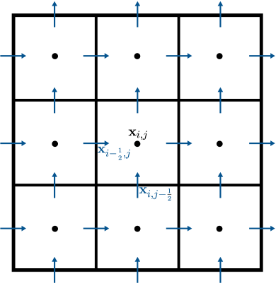
Throughout this paper, we consider the fluid domain as a periodic square with side length . We note that although we use periodic boundary conditions, this is not a major restriction of the IB method, which can readily accommodate physical boundary conditions[34, 35, 36]. The fluid domain is discretized on a uniform Cartesian grid of size , with grid increments . The Eulerian variables are discretized using the MAC staggered-grid discretization introduced by Harlow and Welch [37]. The MAC discretization approximates the pressure at the centers of Cartesian grid cells . The discrete velocity is defined on the centers of the Cartesian grid cell edges with the -component of the velocity located at and the -component of the velocity located at . For an illustration of the MAC discretization, see Figure 1. Following Bao et al.[25], we denote the cell-center degrees of freedom using , and the edge-centered degrees of freedom using . Additionally, we define the nodal degrees of freedom which are located at . Although no discrete Eulerian variables are approximated on , the discrete curl of the velocity field and the discrete scalar potential needed for the DFIB method are both approximated at the grid nodes.
We let denote the discrete gradient operator, the discrete divergence operator, the discrete curl operator, and the discrete Laplace operator. The application of each discrete differential operator is given by
| (5) | ||||
| (6) | ||||
| (7) | ||||
| (8) |
The mappings between degrees of freedom for each discrete differential operator are:
| (9) | ||||
| (10) | ||||
| (11) |
The discrete Laplacian maps a variable to grid locations corresponding to its own degrees of freedom. While we previously described it acting on an edge-centered velocity, it can also be applied to quantities defined at other locations on the Cartesian grid. When applied to a cell-centered quantity, it produces a cell-centered result. Similarly, when used on a quantity defined on the grid nodes, it yields a result also defined on the nodes.
The nonlinear convective term is discretized in advective form using simple second-order accurate central finite differences[38]. We denote the discrete convective term as . Since the velocity components are defined on and are staggered in space, we need to interpolate the vertical velocity component to the x-edge centers where the horizontal component is defined, and interpolate to the y-edge centers where is defined. We perform these interpolations using simple averages. The discretization of the convective term is given by
| (12) |
3.2 Lagrangian Spatial Discretization
In our numerical experiments, we assume the immersed boundary is a smooth closed curve described in physical space by the parametrization at time . We assume the parameter is defined on the interval . To discretize the immersed boundary, we use Lagrangian marker points positioned at , where . We uniformly sample the parameter values along the interval , with a constant increment between consecutive values.
We choose the number of Lagrangian marker points and the increment size based on a desired value of the ratio . This ratio represents the physical distance between Lagrangian markers at the start of a simulation relative to the increment of the background Cartesian grid. We refer to this ratio as the mesh factor and denote it by .
The Lagrangian force densities are similarly discretized using these same parameter values, so that each marker point has an associated Lagrangian force density . The discretization of the Lagrangian force densities will be described in each numerical test below.
3.3 Regularized Delta Functions
In the continuous setting, the immersed boundary method implements fluid-structure interaction through convolutions with singular Dirac delta function kernels as described in equations (3) and (4). The presence of the singular Dirac delta function poses a significant numerical challenge. Thus, the first step in constructing the discretized the IB method is to replace this singular function with a regularized version, , in which the regularization parameter is chosen to be identical to the Eulerian meshwidth . These regularized delta functions are typically expressed in tensor product form:
| (13) |
in which and are one-dimensional kernel functions. Although the formula allows for different functions and in the and directions respectively, in the literature, these are almost always chosen to be the same function, yielding an approximately isotropic kernel function. Indeed, to our knowledge, there are no published descriptions of the immersed boundary method in which the functions and differ. Following Schroeder et al. [32], who showed that composite B-splines produce continuously divergence-free interpolants of discretely divergence-free velocity fields on the MAC grid, our locally divergence-free IB method uses B-spline kernels for and . These kernels differ in polynomial degree by one. In our tests, we also use isotropic kernels where and are identical, allowing us to compare our method with Peskin’s original approach.
Each of the one-dimensional kernels we consider in this paper are derived from two different families of kernel functions. The first family we consider is the B-spline family of kernels, whose invention is attributed to Schoenberg [39], but was mostly popularized by de Boor [40]. B-splines have the attractive property that they can be constructed recursively. This construction starts from the piecewise constant B-spline, :
| (14) |
The rest of the B-spline family is then generated using recursive convolution:
| (15) |
From this recursive identity, many properties of the B-spline family may be concluded. For example, taking the derivative of the B-spline results in a central difference of the B-spline
| (16) |
We remark that equation (15) allows us to infer that the B-spline kernel is made up of nonzero polynomials of degree . The B-spline is times continuously differentiable, is an even function, and is compactly supported with support contained in the interval . One may also use equation to show that as approaches infinity, the sequence of B-splines converges to a rescaled Gaussian [41].
The regularized delta functions constructed using B-spline kernel functions are composite in nature. To interpolate the -component of the velocity or spread the -component of the force, we set and in equation (13). Similarly, to interpolate the -component of the velocity or spread the -component of the force, we set and . This approach ensures that the interpolated velocities resulting from the discretely divergence-free velocities defined on the MAC grid are continuously divergence-free [32]. A proof of this result is provided in section A.1 of the appendix. We detail the discrete velocity interpolation and force spreading operations in the following section.
The second family of one-dimensional kernel functions we consider is the IB family of regularized delta functions. Peskin conceived this family, designing them to be computationally efficient, accurate, and physically relevant [1]. In this work, we employ two kernels from this family: the four-point IB kernel, denoted as , and the relatively new six-point IB kernel, denoted as . The kernel is continuously differentiable and serves as our benchmark for comparing the standard IB method’s performance against the composite B-spline regularized delta functions. The kernel, which we use to implement the divergence-free interpolation and force-spreading scheme developed by Bao et al. [25], satisfies all the properties of the kernel but with improved grid translational invariance. Moreover, the kernel is three times continuously differentiable [42].Regularized delta functions from the IB family are taken to be isotropic. Specifically, we use the same IB kernel function (either or ) for both one-dimensional kernels and in equation (13). This kernel is applied consistently for both and components of the interpolated velocities and spread forces.
3.4 Velocity Interpolation and Force Spreading Operations
This section details the discretization of velocity interpolation and force spreading operations, as described by equations (3) and (4) in the continuous equations of motion. We present two discretization approaches: the non-local DFIB method introduced by Bao et al. [25] and the standard IB method, introduced by Peskin [1]. Both methods replace the singular regularized delta function appearing in the continuous equations with a regularized version, as described in the previous section. The DFIB method, however, introduces an additional step: it first solves for a vector potential, which is then used to ensure that the interpolated velocity field is continuously divergence-free. The force spreading operations for each method are constructed to be adjoint to the corresponding velocity interpolation operation so that energy and momentum are discretely conserved [1].
3.4.1 Non-local DFIB Velocity Interpolation and Force Spreading
We now describe the non-local DFIB velocity interpolation and force spreading operations. Although Bao et al. originally detailed this method in three spatial dimensions [25], we present it here in two spatial dimensions to align with our test scenarios. Following their approach, we first outline the velocity interpolation operation and then construct the force spreading operation as its discrete adjoint. Let be a discretely divergence-free MAC vector field, satisfying:
| (17) |
Let be the discrete mean-flow associated with the velocity field
| (18) |
in which is the area of . Given that is discretely divergence-free, the discrete vector field is discretely curl-free at the cell centers of the Cartesian grid. Analogous to a two-dimensional continuously curl-free vector field, this implies the existence of a scalar potential , defined at the nodes of the Cartesian grid, such that:
| (19) |
or, equivalently:
| (20) |
The potential is unique up to an additive constant. The existence of can be proven by adapting the arguments presented by Bao et al. [25] in three spatial dimenesions to the two-dimensional case considered herein. For periodic boundary conditions on the MAC grid, the discrete divergence of the discrete gradient yields the discrete Laplacian [25]. Consequently, we can solve for the discrete scalar potential by taking the discrete divergence of equation (19). This results in the following discrete scalar Poisson equation, defined at the nodes of the Cartesian grid:
| (21) |
Equivalently, we may also solve for the discrete scalar potential by taking the discrete the discrete curl of equation (20).
Upon obtaining the scalar potential , we interpolate it using a regularized delta function to obtain a continuum scalar potential . Note that IB interpolation amounts to sampling the contiuum field at the locations of the Lagrangian marker points.
| (22) |
We then take the continuous perpendicular gradient of to obtain
| (23) |
The interpolated velocity is then computed from by adding back in the mean flow velocity
| (24) |
So long as the regularized delta function used is at least twice continuously differentiable, Clairut’s theorem guarantees that the interpolated velocity is continuously divergence free. In practice, the discrete scalar potential is never interpolated in equation (23). Instead, the continuum perpendicular gradient of the regularized delta function, , is computed at the nodes of the Cartesian grid and equation (24) is used directly.
The DFIB method’s force spreading operation is constructed as the discrete adjoint of the velocity interpolation operation. This ensures that energy is conserved between Eulerian and Lagrangian interactions, similar to the standard IB method. Bao et al. [25] provided the derivation of the DFIB force spreading operation in three dimensions. Below, we adapt Bao et al.’s derivation to the two-dimensional case for completeness.
Following Bao et al.’s approach, we obtain the two-dimensional DFIB force spreading operation starting from the principle that it should be the discrete adjoint of the velocity interpolation operation. That is,
| (25) |
in which . By replacing both the Eulerian and Lagrangian velocities with their representations based on the discrete scalar potential , the left-hand side of equation (25) becomes
| (26) | ||||
| (27) |
In the equation above, we note that we have applied summation by parts and the assumption of periodic boundary conditions to transfer the discrete perpendicular gradient operator acting on to a discrete curl operator acting on . We introduce the discrete scalar potential on the right hand side of equation (25) by replacing by the divergence-free interpolated velocity
| (28) | ||||
| (29) |
Therefore, equation (25) holds if we set
| (30) |
and
| (31) |
To solve for the Eulerian force density , we make the additional assumption,
| (32) |
This discrete divergence-free condition placed on allows us to obtain the following vector Poisson equation for the Eulerian force density
| (33) |
Upon solving this equation, the unique solution for the Eulerian force density is determined by adding to the computed solution via equation (30). We denote the DFIB force spreading operation using the notation
| (34) |
The DFIB method’s divergence-free assumption on the Eulerian force density is not overly restrictive since only the divergence-free component of f affects the flow. However, the pressure field will differ from that of the physical pressure, as the non-solenoidal forces emanating from the immersed structure are absent.
3.4.2 Local IB Velocity Interpolation and Force Spreading
Given a discrete Eulerian velocity field u, we compute the horizontal and vertical components of the velocity associated with the Lagrangian marker point via
| (35) | ||||
| (36) |
in which . Likewise, given a discrete Lagrangian force density defined at each Lagrangian marker point, we compute the spread force using
| (37) | |||
| (38) |
We remark that both the Eulerian domain and the interval containing the curvilinear coordinate are assumed to be periodic. Consequently, the discrete velocity interpolation and force spreading operations presented above are composite trapezoidal rule approximations of the integrals contained in equations (3) and (4). The convergence rate of the periodic trapezoidal rule is dictated by the convergence rate of the integrand’s Fourier series [43]. Thus, we expect higher accuracy in the discrete force spreading operation when employing a smoother regularized delta function.
3.5 Temporal Discretization
The equations of motion (1)–(4) are discretized in time using a semi-implicit scheme, previously presented for various IB method applications[25]. We describe the timestepping scheme using the notation for the standard IB method, noting that the same scheme applies to the DFIB method. To advance from timestep to , we first approximate the Lagrangian configuration at the midpoint
| (39) |
We then use to approximate the Lagrangian force density at . The updated Lagrangian force density is then passed to the force spreading operator to obtain an approximation for at the midpoint
| (40) |
Next, we solve the following discrete approximation to the momentum equation and incompressibility constraint for and
| (41) | ||||
| (42) |
where is a second-order Adams-Bashforth (AB2) approximation to the advection term at the timestep midpoint
| (43) |
Finally, we compute an approximation to the Lagrangian configuration at using the midpoint approximation
| (44) |
As the nonlinear advective term uses the AB2 scheme, we employ an explicit second-order Runge-Kutta (RK2) scheme for the first timestep, as previously described[1]. While both the DFIB and standard IB methods use the same time-stepping scheme, the DFIB method requires three additional scalar Poisson solves per timestep. We note that in three spatial dimensions, the DFIB method becomes substantially more computationally expensive. It requires nine additional scalar Poisson solves and nine additional scalar interpolation/spreading steps. This makes it approximately twice as costly per timestep in two dimensions and three times more expensive in three dimensions compared to the ordinary IB method [25].
3.6 Area Conservation Measurements
A consequence of the incompressibility of the fluid is that the initial area (or volume) of a closed curve (or surface) remains constant if advected by the fluid. We use this concept to evaluate how well an immersed boundary simulation, combined with a specific regularized delta function, maintains the continuous incompressibility constraint of the fluid. To compute the areas of closed immersed boundaries, we introduce tracer points , positioned according to the initial configuration of the immersed boundary but advected solely by interpolated fluid velocity. This means the tracer points do not generate any Lagrangian forces that are spread back onto the fluid grid. We measure and track the area enclosed by the tracer points by invoking Green’s theorem in the form
| (45) |
in which is the domain enclosed by the closed curve discretized by the tracers and is the interval containing the revelant values of the parameterization parameter . To compute this quantity, we use cubic splines to interpolate the coordinates of the tracers. We then differentiate the spline interpolant of the -coordinate of the tracers and compute the integral given by Green’s theorem by replacing and with their spline representations and integrate these splines exactly. The number of tracer points we use is an integer multiple of the number of Lagrangian marker points employed to discretize the physical immersed boundary. The integer multiple is chosen large enough so that the initial area enclosed by the immersed boundary is computed to within machine precision. In each of our tests, we report the relative change in the area at each timestep
| (46) |
in which is the exact initial area enclosed by immersed boundary.
4 Numerical Tests and Discussion
This section presents empirical tests demonstrating the effectiveness of composite B-splines in preserving areas of immersed boundaries defined by closed curves. To benchmark the composite B-spline regularized delta functions, we compare results with the IB method using the isotropic regularized delta function and the (non-local) DFIB method using the isotropic regularized delta function. All physical quantities in this paper are reported using the centimeter-gram-second (CGS) unit system. The fluid is characterized by a constant density of and a dynamic viscosity value of , unless explicitly stated otherwise for a particular simulation.
4.1 Advecting an Immersed Boundary Using Taylor Vortices
We first test the ability of the interpolation scheme to reconstruct incompressible material trajectories for a case that does not involve fluid-structure interaction by comparing the standard IB method and the DFIB method when applied to advecting Lagrangian tracers according to a Taylor-Green vortex flow on the periodic unit square. The associated velocity and pressure fields are given by:
| (47) | ||||
| (48) | ||||
| (49) |
The tracers are intialized so that they discretize the circle centered at and radius of . We emphasize that the tracers are purely advected using the interpolation strategies of both the IB and DFIB methods. No Lagrangian force densities are spread onto the Cartesian grid.
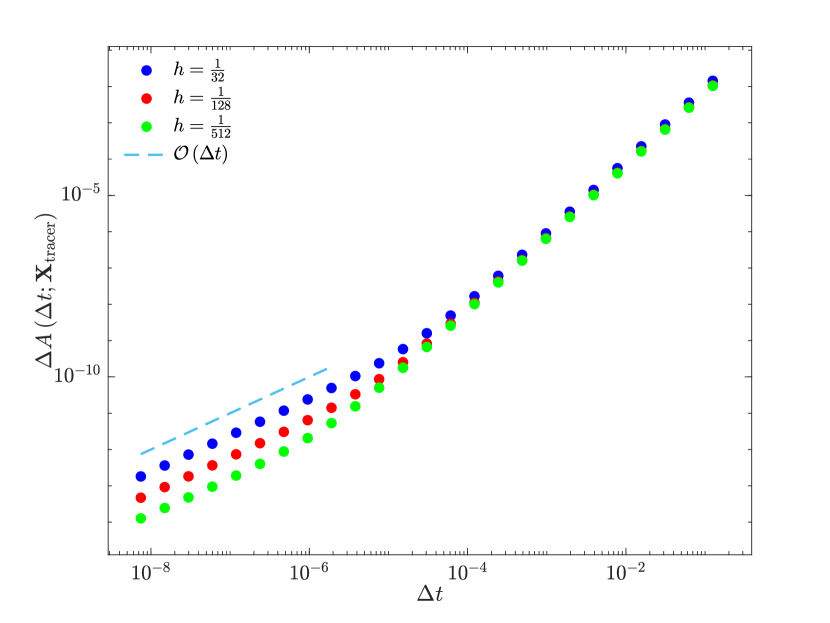
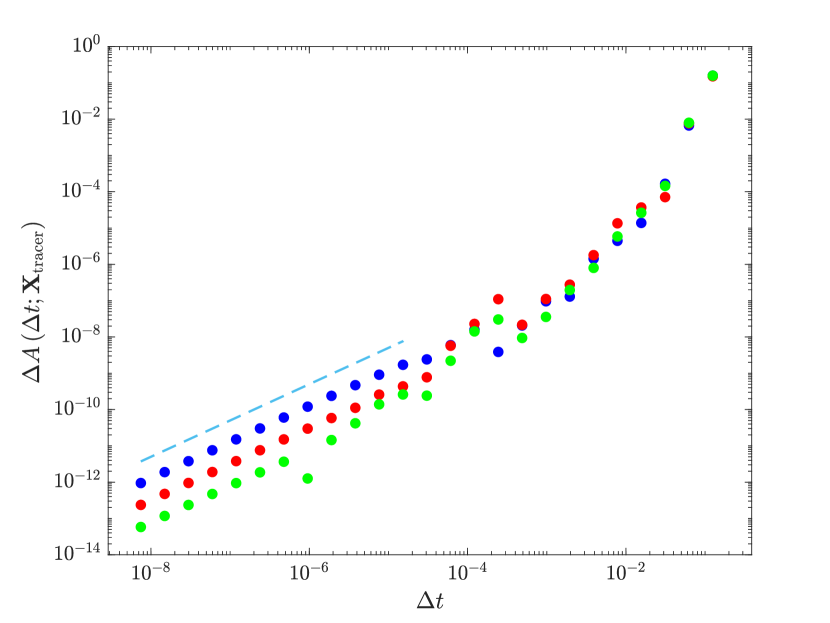
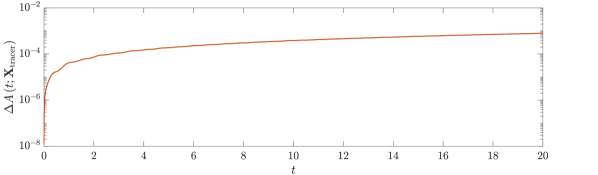
To evaluate area conservation properties, we simulate advection of the tracers on a uniform grid with increment . We use eight time step sizes: , and . For each method and choice of regularized delta function, we compute the temporal mean of the relative area error over the interval . In this context, area computation errors may arise from two different sources: (1) the interpolated velocity field not being continuously divergence-free, or (2) the time-stepping scheme introducing errors in tracer positions. Both the DFIB and IB methods update the positions of the tracers using the explicit midpoint rule, which has a global truncation error that is second-order accurate. Consequently, we expect the errors introduced by the time-stepping scheme to be of order until the error associated with the incompressibility of the interpolated velocity field becomes dominant. Additionally, there are errors associated with the cubic spline interpolation of the tracer points. However, we’ve observed that these interpolation errors are much smaller in magnitude than the errors committed by our choice of time stepping scheme.

The results are illustrated in Figure 2. The relative area errors of the DFIB and IB methods implemented with each of the composite B-splines, except the discontinuous kernel, are completely superimposed and exhibit second-order convergence with respect to the time step size . For larger time step sizes, the IB method with the and regularized delta functions also exhibits second-order convergence. However, for the kernel, upon decreasing the time step size below , the relative area error begins to level off as the error associated with the incompressibility of the interpolated velocity dominates. Similarly, the relative error levels off for the kernel below a time step size of .
Although the kernel provides a continuously divergence-free interpolant, we observe that the error levels off as decreases. This unexpected behavior can be attributed to the discontinuous nature of the resulting interpolated velocity field. These discontinuities in the interpolated velocity field lead to discontinuities in the resulting time derivatives, which in turn reduce the asymptotic local truncation error of the explicit midpoint rule to only first-order in time. Consequently, the asymptotic global truncation error remains as approaches zero. Supplemental analysis regarding this phenomenon is provided in section A.3 in the appendix.
4.2 A Pressurized Circular Membrane at Equilibrium
Next we consider a FSI problem in which the IB method is used to simulate a quasi-static pressurized membrane which is initialized in its circular equilibrium configuration with center and radius immersed the periodic unit square , with zero initial background flow. The Lagrangian force density is described by
| (50) |
We discretize this equation using centered, second-order accurate finite differences yielding
| (51) |
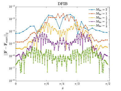
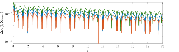
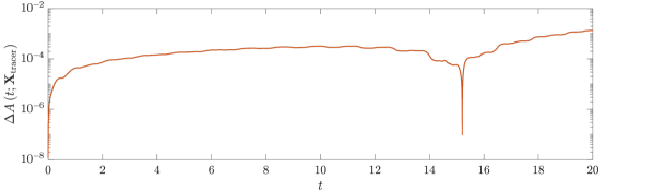
This formulation models the Lagrangian markers as being linked by linear springs with zero rest lengths and a uniform stiffness . In our simulations of the quasi-static pressurized membrane, we use a stiffness value of and a fixed time step size of , in which . Additionally, unless otherwise noted, we set the Lagrangian mesh factor . Because the immersed membrane is intialized at equilibrium, we consider any deviation from the initial area enclosed by the membrane to be attributed to errors associated with spatial discretization of the IB method employed. Griffith [19] simulated a pressurized membrane at equilibrium using the IB method in which the Eulerian variables were discretized according to the MAC scheme [37] and the velocity interpolation and force spreading operators were implemented using Peskin’s four-point delta function [1]. Griffith found that although the MAC discretization of the IB method exhibited better volumer conservation properties compared to a collocated discretization, the IB method discretized on the MAC grid still exhibited significant volume errors. Bao et al. found that so long as the the immersed boundary was resolved enough, the DFIB method was able to maintain the initial volume of the immersed boundary to within machine precision [25] while the IB method produced volume errors which leveled off at constant values even as the immersed membrane was further refined. In Fig. 3 we compare the DFIB method implemented with the six-point IB kernel to the standard IB method implemented with the four-point IB and composite B-spline regularized delta functions.

Consistent with the findings of Bao et al., we observe that the DFIB method preserves the initial area of the circle to within machine precision throughout the simulation. Likewise, the two composite B-spline pairs with the highest regularity, and , also maintain the initial area of the circle to within machine precision. Although composite B-spline pairs of lower regularity do not achieve the same level of accuracy as their higher regularity counterparts, they still significantly outperform the standard four-point IB kernel, with the least regular composite B-spline pairing, , performing about an order of magnitude better than the standard four-point kernel. Furthermore, we note that the relative area errors for the and regularized delta functions level off about where their mean errors level off in the pure advection test illustrated in Fig 2.
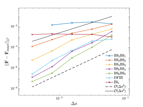
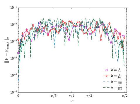
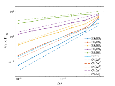
Since the membrane is intialized in its circular configuration, the exact Lagrangian force density is given by , in which is the radius of the circle and is the circle’s unit outward pointing normal vector. Fig 4 presents the pointwise error in the computed steady-state Lagrangian force densities using the , , and regularized delta functions and the DFIB method over the first quadrant of the circle. We compute the error using the norm of difference between the exact Lagragian force densities and the computed steady-state Lagrangian force densities. Fig 5 illustrates the convergence rates of the Lagragian force densities in the sense of the grid norm taken over the circle
| (52) |
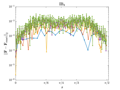
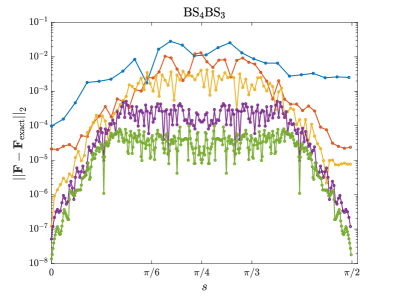
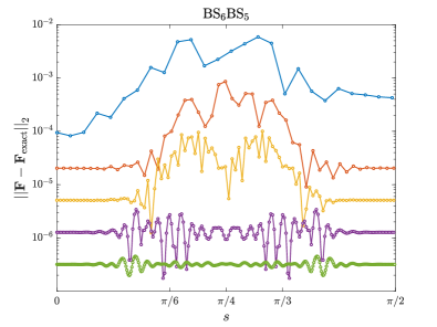
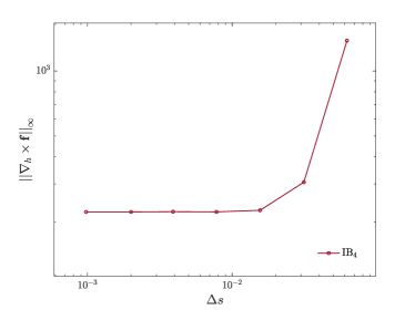
We observe varying convergence behaviors in Lagrangian force densities across different kernels and methods. The composite B-splines, excluding only the discontinuous kernel, empirically produce Lagrangian force densities that converge pointwise under solely Lagrangian grid refinement. This pointwise convergence is demonstrated for the and kernels, as well as the DFIB method in Fig 4. In contrast, the kernel does not yield pointwise convergent Lagrangian force densities under these conditions. In fact, for the kernel, this lack of convergence persists even under simultaneous refinements of both grid sizes and time step size, as shown in Fig 6.
Examining the grid norm convergence of the Lagrangian force densities, as shown in Fig 5, we find that the , , , and regularized delta functions, along with the DFIB method, all provide convergence under Lagrangian grid refinement, with the more regular kernels generally producing smaller errors. The less regular kernel appears to yield convergence rates proportional to , while the more regular composite B-spline kernels and DFIB method produce asymptotic rates proportional to . Notably, both the regularized delta function and the kernel fail to produce convergent Lagrangian force densities under only Lagragian grid refinement. The inaccuracies associated with the kernel can be attributed to the discontinuous nature of the interpolated velocity in both time and the curvilinear coordinate . These discontinuities in the interpolated velocity field propagate to the Lagrangian marker positions, resulting in jump discontinuities in their trajectories with respect to both and . Consequently, large localized errors arise in the computed Lagrangian force densities near these discontinuity points. A more detailed discussion of the discontinuities in the interpolated velocity obtained using the kernel is presented in section A.1 of the appendix.
For the pressurized membrane problem, we note that as long as the time step is simultaneously refined with the Cartesian grid increment , the errors in the Lagrangian force densities using the IB method with composite B-spline regularized delta functions (excluding ) and the DFIB method appear to depend only on the value of .
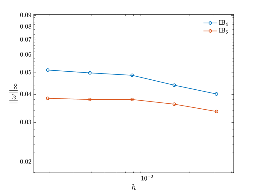
Figs. 3, 4, and 5 indicate that the regularity of the kernel function employed impacts the errors associated with volume conservation and the computation of the Lagrangian force densities. Errors present in either quantity indicate the generation of spurious, non-physical flows which advect Lagrangian markers to new positions in space, subsequently deteriorating the accuracy of the Lagrangian force densities and area measurements. Similar spurious flows were described by Kaiser et al. in their IB simulations of the mitral valve [7]. To investigate these spurious flows, we begin by examining the discrete vorticity associated with the simulation. We choose to analyze the vorticity since its associated equation decouples from the pressure on the periodic MAC grid. This is because, on the periodic MAC grid, we have , just like the continuum formulation. By taking the discrete curl of equation (41), we observe that vorticity can be generated in the discrete setting only if the discrete curl of the Eulerian force density is non-zero. Fig. 7 illustrates the vorticity and flow fields present in the pressurized membrane problem early in the simulation at using the , , and regularized delta functions, as well as the DFIB method. We chose the early time of to observe what errors in the flow field are introduced early in the simulation. However, we note that the flow features do not change significantly over time.
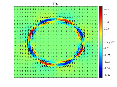
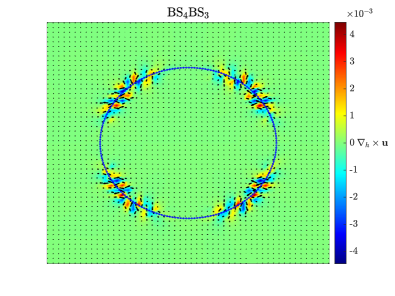
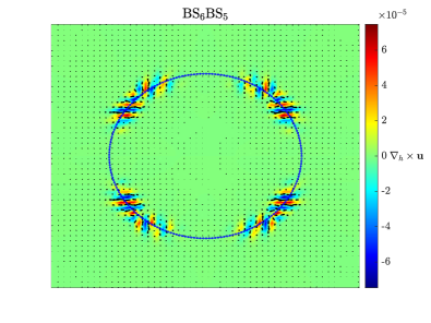
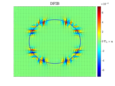
We observe that for each regularized delta function employed, there are regions of relatively high vorticity along the boundary of the circle. Moreover, the magnitude of the vorticity seems to depend on the regularity of the kernel function employed. The isotropic kernel produces the largest and most distributed vorticity values while the composite kernel yields the smallest vorticity values. The DFIB method, which employs employs a interpolant, and the IB method with the kernel produces intermediate vorticity values, with the DFIB method generating voriticty values about an order of magnitude less than the IB method implemented with the kernel.
We remark that the continuous formulation of the IB method, assuming the kernels and in equation (13) are at least , the force associated with the equilibrium pressurized membrane should induce zero vorticity. This is because the curl of the Eulerian force density is given by
| (53) | ||||
| (54) | ||||
| (55) | ||||
| (56) | ||||
| (57) |
Note that the equality between equations (55) and (56) is implied by the divergence theorem. However, in the discrete setting, Fig 7 demonstrates that the discrete vorticity is nonzero, implying that the discrete curl of the Eulerian force density must also be nonzero.
To analyze this discrepancy, we take the discrete curl of the continuous force spreading operator for both the IB and DFIB methods for the pressurized membrane at equalibrium. Starting with the IB method, we assume that the regularized delta function is given by a composite B-spline formulation in which
| (58) |
in the horizontal direction, and
| (59) |
in the vertical direction. Using this definition, the discrete curl of the Eulerian force density is given by
| (60) |
| (61) |
Using identity (16), we may rewrite the centered differences of the B-splines as
| (62) | |||
| (63) |
Upon making this substitution and identifying the Lagrangian force density with , equation (61) becomes
| (64) |
Applying the divergence theorem to equation (64), we obtain
| (65) | ||||
| (66) |
in which the double integral above is taken over the interior of the unit circle. Therefore, we may conclude that when the force spreading operator is made exact, the composite B-spline regularized delta functions yield an Eulerian force density that is discretely curl-free, like its continuous counterpart. This implies that the vorticity should vanish as we make further refinements to the force spreading operator, assuming the Lagragian markers are held in place. Once the voriticty, and hence flow advect Lagragian markers away from the boundary of the circle, other errors may propogate.
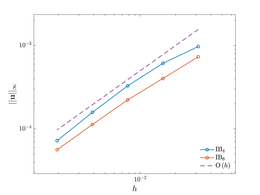
If instead the regularized delta function is isotropic, like the regularized delta function, the discrete curl of the continuous force spreading operator contains errors of size . This occurs because the central difference of the kernels that appears in equation (64) is generally a approximation of the kernel’s derivative, due to the argument of the kernel being scaled with respect to . An order of magnitude analysis then suggests that in this case, vorticity ought to scale like , indicating that the vorticity will not converge under simultaneous grid refinement. Although vorticity does not appear to converge under grid refinement when using isotropic kernels, the velocity does converge to zero at a linear rate[44] proportional to . We provide empirical evidence and further theoretical discussions regarding isotropic regularized delta functions in section A.2 of the appendix.
Since the discrete curl of the Eulerian force density associated with the DFIB method satisfies equation (31), the divergence theorem implies that the Eulerian force density is discretly curl free for the pressurized membrane problem. Therefore, similar for the composite B-splines, we expect the vorticity to converge to zero as spreading operator converges to its exact value.
To test the robustness of this analysis in the fully discrete setting, we compute the discrete curl of the force spreading operator at the beginning of the simulation before the velocity is subsequently computed and the Lagragian markers are advected. Fig 8 shows the maximum values of the discrete curl of Eulerian force density as a function of the Lagrangian parameter grid size , and the particular regularized delta function employed.
As predicted, both the composite B-spline regularized delta functions and DFIB methods produce force spreading operators whose curl vanishes solely under Lagrangian grid refinement. The convergence rate is strongly influenced by the regularity of the kernel function. This aligns with expectations, as we approximate the line integral associated with the force spreading operator using the periodic trapezoidal rule. The asymptotic convergence rate of periodic trapezoidal rule depends on the integrand’s regularity [43]. Specifically, for a integrand with , the convergence rate should scale approximately as . For discontinuous integrands, the expected convergence rate is first-order. Notably, the empirical error rates for each kernel closely match the expected error rates predicted for the periodic trapezoidal rule. Additionally, we observe that the curl of the force spreading does not converge with Lagrangian grid refinement for the kernel, as expected.
Given that our finite difference approximation of F (equation (51)) is only second-order accurate, the close agreement between the expected periodic trapezoidal rule and observed error rates might seem surprising. However, the higher-order terms in the Taylor series expansion of the error are all proportional to even derivatives of the parameterization. Each error term is thus directly proportional to the circle’s normal vector. Consequently, the divergence theorem implies that these higher-order error terms also vanish as the Lagrangian grid is refined.
4.3 A Parameterically Excited Membrane
In this section we use the IB and DFIB methods to simulate a parametrically excited membrane whose elastic stiffness varies periodic in time. The Lagrangian force density associated with the membrane is given by
| (67) | ||||
| (68) |
The membrane is initially configured as a perturbation of the a circle radius centered in a periodic square fluid domain . The intial configuration of the membrane is described by the parameterization
| (69) |
where is the unit outward pointing normal vector of the unit circle. This model problem, introduced by Cortez et al. [45, 46], serves as a simple representation of an active immersed material driven by a periodic forcing. Cortez et al. performed a Floquet analysis of this problem, in which the integer parameter identifies the wavenumber of the Floquet mode under consideration. The parameters and control the amplitude and frequency of the stiffness oscillation, respectively. The parameter a small parameter used to linearize the equations of motion.
Here, we consider two distinct time evolutions of the forced membrane using parameter values consistent with Bao et al.’s tests [25]. Guided by Cortez et al.’s Floquet analysis, Bao et al. examined two parameter combinations: one resulting in damped oscillations, and another leading to growing oscillations that are eventually stabilized by nonlinearities. These parameter values are reproduced in Table 1 for reference.
| 1 | 0.15 | 5 | 1 | 10 | 10 | 2 | 0.05 | 0.4 | (damped oscillation) |
| 1 | 0.15 | 5 | 1 | 10 | 10 | 2 | 0.05 | 0.5 | (growing oscillation) |
The background Cartesian grid is discretized using a uniform increment and the Lagragian markers are intialized so that the physical distance separating them is roughly in the equilibrium configuration so that . Similar to the static pressurized membrane problem we monitor errors in area conservation using the method desribed in section 3.6. For this problem, the exact area enclosed by the initial configuration of the immersed boundary is given by
| (70) |
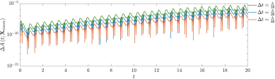
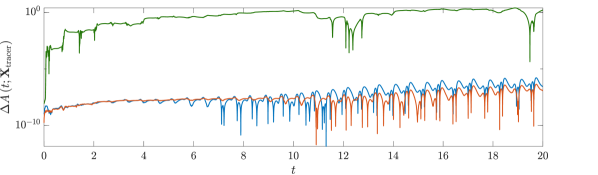
For each set of parameter values, we examine three different time step sizes: and . Since we use a second-order time stepping scheme, we anticipate that the error in area computation will scale as . However, this scaling may be superseded if errors associated with the approximation of the force spreading operator or velocity interpolation become dominant factors. For each dynamic problem, we observed that area errors associated with composite B-splines of regularity or greater produced were roughly identical to the area errors produced by the DFIB method. Thus, to avoid redundancy, we present only the results of the , , and composite B-spline regularized delta functions. Fig 9 shows the relative area errors of these composite B-splines along side with the relative area errors produced by the kernel and DFIB method.
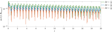
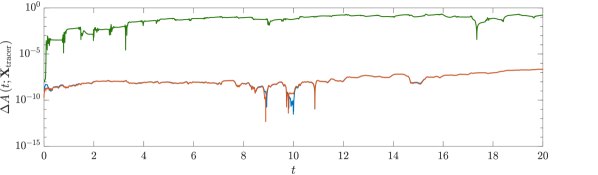
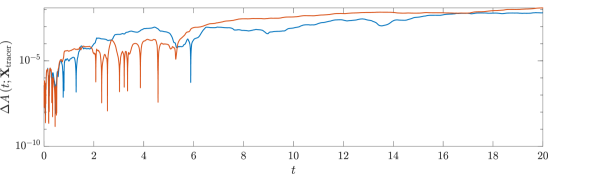
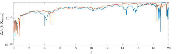
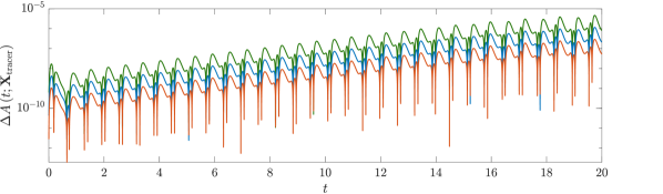
The area errors for the were not included for the time step size because the simulation became unstable. For composite B-spline regularized delta functions with regularity or higher, as well as for the DFIB method, we observe that the area errors are primarily influenced by the time-stepping scheme. This is evidenced by the consistent decrease in area error for both approaches. For the kernel, all of the relative area errors super impose atop each other indicating that the error is dominated by the velocity interpolation error associated with the kernel. The composite kernel performs relatively poorly compared to the more regular composite B-splines at the largest time step size of . When the time step size is reduced by a factor of 2, the kernel produces more accurate error estimates. However, with further reduction in time step size, the errors remain constant, indicating that the error associated with the approximation of the force spreading operator becomes dominant beyond this point. The discontinuous kernel produces area errors of relatively consistent magnitude across all stable time step sizes. This consistency suggests that for the kernel, the error in approximating the force spreading operator dominate. Recall that the kernel generates an interpolated velocity field which is discontinuous resulting in first order local truncation errors and thus global truncation errors over the duration of a simulation. The trends for each kernel function similarily reproduced for the resonant case of the parametrically excited membrane; however, the relative area errors a slightly larger due to larger time-stepping errors associated with the growing amplitude of the membrane’s oscillation. These results are presented in Fig 10.
5 Conclusions
In this study, we have introduced and analyzed the use of composite B-spline regularized delta functions to improve the volume conservation properties of the IB method. These B-spline kernels provide locally divergence-free velocity interpolants, and this study shows that when used with the IB method, they are also effective force spreaders as well. Composite B-spline regularized delta functions address a long-standing challenge associated with the IB method: the poor volume conservation of closed immersed structures, particularly evident in simulations of pressurized, closed membranes which tend to lose volume at a rate constant rate proportional to the pressure jump across the immersed boundary.[18, 19]
Our numerical experiments demonstrate that composite B-spline regularized delta functions significantly enhance the volume conservation properties of the IB method. Additionally, volume conservation errors are comparable and even smaller for sufficiently regular kernels compared to the DFIB method. Recall that the DFIB method also requires a kernel function to have sufficient regularity, at least twice continuously differentiable, to be effective at mitigating volume conservation errors. Composite B-splines of less regularity are less competitive for volume conservation, but still produce volume errors smaller than those comitted when using the kernel.
We observed for tests of pure advection, composite B-splines of regularity and above acheived area errors that were proportional to the expected time discretization error, matching the performance of the DFIB method. For relatively large timestep sizes, the area errors associated with the kernel also acheives second-order convergence. However, upon reaching smaller timestep sizes, the compressibility of the interpolated velocity eventually dominates the relative area error.
For the quasi-static pressurized membrane problem, the more regular composite B-splines kernels, , , and , maintained the initial area to within machine precision, similar to the DFIB method. Less regular splines acheived better area conservation comparted to the regularized delta function, which tends to produce a linear rate of error loss in time[18, 19]. We examined how the error depends on the regularity of the kernel used for divergence-free interpolation. Our analysis revealed that differences in errors were primarily due to the approximation quality of the force spreading operator. To support this conclusion, we analyzed the discrete curl of the spreading operator. We demonstrated that the curl of the force density, which generates spurious vorticity, converges to zero at a rate consistent with theoretical periodic trapezoidal rule error estimates. Importantly, this convergence rate is dependent on the regularity of the integrand. For isotropic kernels, like the kernel, the discrete curl of the force spreading operator consistently commits errors. Consequently, the vorticity does not converge under grid refinement. In our analysis of the pressurized membrane problem, we also evaluated the quality of the computed Lagrangian force densities. We found that, similar to the DFIB method, the use of composite B-spline regularized delta functions produced pointwise convergent Lagrangian forces. The error in the Lagrangian forces decreased with more regular kernel functions and appeared to depend primarily on the quality of the force spreading approximation. In contrast, the kernel was unable to produce convergent Lagrangian force densities, even when both temporal and spatial grids were refined simultaneously.
In our dynamic simulations of parametrically excited membranes, we observed that composite B-splines of regularity class or higher produced results essentially identical to the DFIB method. For these higher-regularity kernels, errors were primarily dominated by time-stepping rather than spatial discretization. Lower-regularity composite B-splines were less competitive, as they provided poorer approximations of the force spreading operator. The discontinuous kernel performed the worst, yielding the least accurate volume estimates. Moreover, for the largest timestep size of , simulations using this kernel became unstable. The interpolation and force spreading operator errors were dominant for the kernel at each choice of time-step size.
Our findings indicate that composite B-spline regularized delta functions require a minimum level of regularity to be competitive with the DFIB method developed by Bao et al [25]. For practical implementations of the IB method, we recommend the kernel. This kernel represents the least regular B-spline with the smallest set of support that consistently performed comparably to the DFIB method across all our tests. However, we note that the dependence on B-spline regularity may largely be a consequence of our use of the periodic trapezoidal rule to approximate the line integral associated with the force spreading operator. An important direction for future work is to analyze the performance of the method using quadrature rules that are less sensitive to the regularity of the integrand. This would allow force spreading operations to be made more accurate for the less regular composite B-spline kernels, potentially offering a better balance between accuracy and computational efficiency.
Implementing the IB method using composite B-spline regularized delta functions offers a compelling alternative to existing approaches for improving volume conservation in the IB method. It achieves high accuracy without the computational overhead of the DFIB method, making it particularly attractive for large-scale, three-dimensional simulations where computational efficiency is crucial. Importantly, adopting this approach requires only a single modification to existing IB code: changing the delta function implementation. This minimal change allows users to significantly enhance their simulations with minimal effort, making it an accessible improvement for a wide range of IB method applications.
6 Acknowledgments
Cole Gruninger is grateful for support from the Department of Defense (DoD) through the National Defense Science and Engineering Graduate (NDSEG) Fellowship Program. Boyce E. Griffith gratefully acknowledges support from the National Institutes of Health (NIH) under grant numbers NIH U01HL143336, NIH R01HL157631, and NIH R41GM136084, as well as the National Science Foundation (NSF) under grant numbers OAC 1652541 and OAC 1931516.
REFERENCES
- [1] C.S. Peskin. The immersed boundary method. Acta Numerica, 11:479–517, 2002.
- [2] B.E. Griffith, X.Y. Luo, D.M. McQueen, and C.S. Peskin. Simulating the fluid dynamics of natural and prosthetic heart valves using the immersed boundary method. Int. Jour. of Applied Mech., 01(01):137–177, 2009.
- [3] A. Hasan, E.M. Kolahdouz, A. Enquobahrie, T.G. Caranasos, J.P. Vavalle, and B.E. Griffith. Image-based immersed boundary model of the aortic root. Medical Engineering & Physics, 47:72–84, 2017.
- [4] B.E. Griffith. Immersed boundary model of aortic heart valve dynamics with physiological driving and loading conditions. International Journal for Numerical Methods in Biomedical Engineering, 28(3):317–345, 2012.
- [5] W.W. Chen, H. Gao, X.Y. Luo, and N.A. Hill. Study of cardiovascular function using a coupled left ventricle and systemic circulation model. Journal of Biomechanics, 49(12):2445–2454, 2016. Cardiovascular Biomechanics in Health and Disease.
- [6] L. Crowl and A.L. Fogelson. Analysis of mechanisms for platelet near-wall excess under arterial blood flow conditions. Journal of Fluid Mechanics, 676:348–375, 2011.
- [7] A.D. Kaiser, D.M. McQueen, and C.S. Peskin. Modeling the mitral valve. International Journal for Numerical Methods in Biomedical Engineering, 35(11):e3240, 2019.
- [8] T. Skorczewski, B.E. Griffith, and A. Fogelson. Multi-bond models for platelet adhesion and cohesion. In Anita L.T. and Sarah O.D., editors, Biological Fluid Dynamics: Modeling, Computations, and Applications, volume 648, chapter 8, pages 149–172. American Mathematical Society, 2014.
- [9] A.L. Fogelson and R.D. Guy. Immersed-boundary-type models of intravascular platelet aggregation. Computer Methods in Applied Mechanics and Engineering, 197(25):2087–2104, 2008.
- [10] S.K. Jones, R. Laurenza, T.L. Hedrick, B.E. Griffith, and L.A. Miller. Lift vs. drag based mechanisms for vertical force production in the smallest flying insects. Journal of Theoretical Biology, 384:105–120, 2015.
- [11] A. Santhanakrishnan, S.K. Jones, W.B. Dickson, M. Peek, V.T. Kasoju, M.H. Dickinson, and L.A. Miller. Flow structure and force generation on flapping wings at low Reynolds numbers relevant to the flight of tiny insects. Fluids, 3(3), 2018.
- [12] S. Alben, L.A. Miller, and J. Peng. Efficient kinematics for jet-propelled swimming. Journal of Fluid Mechanics, 733:100–133, 2013.
- [13] A.P.S Bhalla, R. Bale, B.E. Griffith, and N.A. Patankar. Fully resolved immersed electrohydrodynamics for particle motion, electrolocation, and self-propulsion. Journal of Computational Physics, 256:88–108, 2014.
- [14] E.D. Tytell, C. Hsu, and L.J. Fauci. The role of mechanical resonance in the neural control of swimming in fishes. Zoology, 117(1):48–56, 2014.
- [15] R. Bale, I.D. Neveln, A.P.S. Bhalla, M.A. MacIver, and N.A. Patankar. Convergent evolution of mechanically optimal locomotion in aquatic invertebrates and vertebrates. PLOS Biology, 13(4):1–22, 04 2015.
- [16] A.P. Hoover, B.E. Griffith, and L.A. Miller. Quantifying performance in the medusan mechanospace with an actively swimming three-dimensional jellyfish model. Journal of Fluid Mechanics, 813:1112–1155, 2017.
- [17] N. Nangia, R. Bale, N. Chen, Y. Hanna, and N.A. Patankar. Optimal specific wavelength for maximum thrust production in undulatory propulsion. PLOS ONE, 12(6):1–23, 2017.
- [18] C.S. Peskin and B.F. Printz. Improved volume conservation in the computation of flows with immersed elastic boundaries. Journal of Computational Physics, 105(1):33–46, 1993.
- [19] B.E. Griffith. On the volume conservation of the immersed boundary method. Communications in Computational Physics, 12(2):401–432, 2012.
- [20] R. Cortez and M. Minion. The blob projection method for immersed boundary problems. Journal of Computational Physics, 161(2):428–453, 2000.
- [21] R.J. LeVeque and Z. Li. The immersed interface method for elliptic equations with discontinuous coefficients and singular sources. SIAM Journal on Numerical Analysis, 31(4):1019–1044, 1994.
- [22] Z. Li and M. Ming-Chih Lai. The immersed interface method for the navier–stokes equations with singular forces. Journal of Computational Physics, 171(2):822–842, 2001.
- [23] R.J. LeVeque and Z. Li. Immersed interface methods for stokes flow with elastic boundaries or surface tension. SIAM Journal on Sci. Comp., 18(3):709–735, 1997.
- [24] L. Lee and R.J. LeVeque. An immersed interface method for incompressible navier–stokes equations. SIAM Journal on Scientific Computing, 25(3):832–856, 2003.
- [25] Y. Bao, A. Donev, B.E. Griffith, D.M. McQueen, and C.S. Peskin. An immersed boundary method with divergence-free velocity interpolation and force spreading. Journal of Computational Physics, 347:183–206, 2017.
- [26] P. A. Raviart and J. M. Thomas. A mixed finite element method for second-order elliptic problems. In I. Galligani and E. Magenes, editors, Mathematical Aspects of Finite Element Methods, volume 606 of Lecture Notes in Mathematics. Springer, Berlin, Heidelberg, 1977.
- [27] J. A. Evans and T. J. R. Hughes. Isogeometric divergence-conforming b-splines for the steady navier-stokes equations. Mathematical Models and Methods in Applied Sciences, 23(8):1421 – 1478, 2013.
- [28] G.G. Tong, D. Kamensky, and J.A. Evans. Skeleton-stabilized divergence-conforming b-spline discretizations for incompressible flow problems of high reynolds number. Computers and Fluids, 248:105667, 2022.
- [29] H. Casquero, Y.J. Zhang, C. Bona-Casas, L. Dalcin, and H. Gomez. Non-body-fitted fluid–structure interaction: Divergence-conforming b-splines, fully-implicit dynamics, and variational formulation. Journal of Computational Physics, 374:625–653, 2018.
- [30] H. Casquero, C. Bona-Casas, D. Toshniwal, T.J.R. Hughes, H. Gomez, and Y.L. Yongjie Jessica Zhang. The divergence-conforming immersed boundary method: Application to vesicle and capsule dynamics. Journal of Computational Physics, 425:109872, 2021.
- [31] D.C. Handscomb. Spline Representation of Incompressible Flow. IMA Journal of Numerical Analysis, 4(4):491–502, 1984.
- [32] C. Schroeder, R. Roy Chowdhury, and T. Shinar. Local divergence-free polynomial interpolation on MAC grids. Journal of Computational Physics, 468:111500, 2022.
- [33] R. Roy-Chowdhury, T. Shinar, and C. Schroeder. Higher order divergence-free and curl-free interpolation on MAC grids. Journal of Computational Physics, 503:112831, 2024.
- [34] B. E. Griffith. Immersed boundary model of aortic heart valve dynamics with physiological driving and loading conditions. International Journal for Numerical Methods in Biomedical Engineering, 28(3):317–345, 2012.
- [35] B. E. Griffith. An accurate and efficient method for the incompressible Navier-Stokes equations using the projection method as a preconditioner. Journal of Computational Physics, 228(20):7565–7595, 2009.
- [36] B. E. Griffith, X. Y. Luo, D. M. McQueen, and C. S. Peskin. Simulating the fluid dynamics of natural and prosthetic heart valves using the immersed boundary method. International Journal of Applied Mechanics, 1(1):137–177, 2009.
- [37] F.H. Harlow and J.E. Welch. Numerical calculation of time-dependent viscous incompressible flow of fluid with free surface. Physics of Fluids, 8(12):2182–2189, 1965.
- [38] W. E and L. Jian-Guo. Projection method III: Spatial discretization on the staggered grid. Mathematics of Computation, 71(237):27–47, 2001.
- [39] I.J. Schoenberg. Contributions to the problem of approximation of equidistant data by analytic functions. part a.- on the problem of smoothing or graduation. a first class of analytic approximation formulae. part b.- on the second problem of osculatory interpolation. a second class of analytic approximation formulae. Quaterly of Applied Mathematics, 4(1):45–99 and 112–141, 1946.
- [40] C. de Boor. A Practical Guide to Splines, volume 27 of Applied Mathematical Sciences. Springer-Verlag, New York, 1978.
- [41] M. Unser, A. Aldroubi, and M. Eden. On the asymptotic convergence of b-spline wavelets to gabor functions. IEEE Transactions on Information Theory, 38(2):864–872, 1992.
- [42] Y. Bao, J. Kaye, and C.S. Peskin. A gaussian-like immersed-boundary kernel with three continuous derivatives and improved translational invariance. Journal of Computational Physics, 316:139–144, 2016.
- [43] J.P. Boyd. Chebyshev and Fourier Spectral Methods. Dover Publications, Mineola, New York, 2 edition, 2001. Chapter 19, p. 458.
- [44] Y. Mori. Convergence proof of the velocity field for a Stokes flow immersed boundary method. Comm. Pure and Appl. Math., 61(9):1213–1263, 2008.
- [45] R. Cortez, C.S. Peskin, J.M. Stockie, and D. Varela. Parametric resonance in immersed elastic boundaries. SIAM Journal on Applied Mathematics, 65(2):494–520, 2004.
- [46] W. Ko and J.M. Stockie. Correction to "parametric resonance in immersed elastic boundaries", 2014.
Appendix A Appendix
A.1 Local divergence-free interpolation using composite B-splines
In this section of the appendix, we prove that if composite B-splines interpolate a velocity field which is discretely divergence-free on the MAG grid, then the interpolated velocity is continuously divergence-free. Let be a discretely divergence free velocity field. We assume that the velocity field is periodic in space. However, this proof also applies to non-periodic domains, provided that the location where the velocity is being interpolated, , is a distance from boundary of the computational domain which is greater than the width of the support of the revelant B-spline kernel.
| (71) | ||||
| (72) |
Taking the continuous divergence of with respect to , we obtain
| (73) |
Using the derivative identity (16) associated with the B-spline sequence, the continuous divergence may be expanded to
| (74) | ||||
| (75) |
Applying summation by parts to the sums and transforms the above into
| (76) | |||
| (77) |
which is zero according to our assumption that is discretely divergence free.
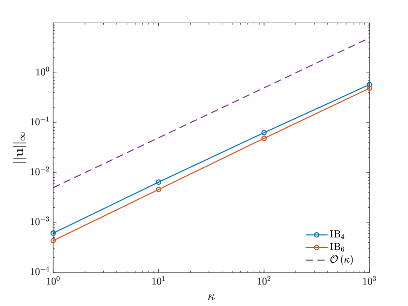
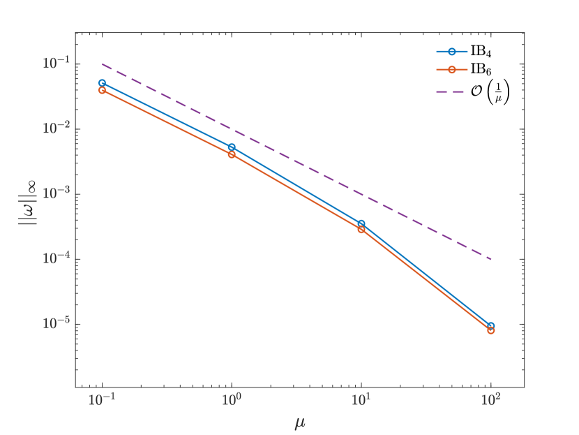
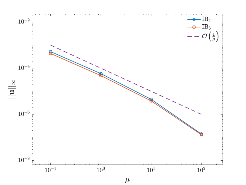
A.2 Analysis of spurious flows associated with isotropic kernels
In section 4.2, we observed that the force density spread by the isotropic regularized delta function constructed using the kernel generated significant spurious flows even when the Lagrangian force density was conservative. More specifically, our analysis focused on a pressurized membrane at equilibrium, where the Lagrangian force density is given by , with representing the membrane’s stiffness and the radius of the membrane’s circular equilibrium configuration. We observed that using isotropic regularized delta functions to spread this force resulted in substantial spurious flows near the circle’s boundary.
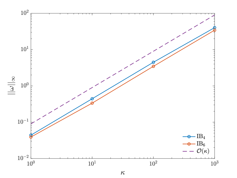
In the subsequent discussion, we posited that the induced vorticity resulting from the spread force does not converge under grid refinement and scales proportionally to , where is the fluid’s dynamic viscosity. This section of the appendix aims to provide a heuristic argument supporting this claim and present additional empirical evidence, further elaborating on our findings for isotropic regularized delta functions.
To analyze these spurious flows, we work in the context of the equilibrium pressurized membrane problem. We once again examine the discrete curl of the force spreading operator, assuming the line integral associated with it is exact. This approach is chosen because, theoretically, for no flow to be induced, the discrete curl of the force spreading operator should vanish assuming the resulting force being spread is indeed a conservative vector field. Taking the discrete curl of the force spreading operator when using an isotropic regularized delta function yields:
| (78) |
Applying the divergence theorem to this equation, we can see that the the curl of the Eulerian force density is given by
| (79) | ||||
| (80) |
in which the double integral above is taken of the interior of the circle. Clearly, if the central differences of the kernels, e.g., , were equivalent to their true derivatives or even good approximations of those derivatives, the curl of the Eulerian force density would be zero or relatively small, respectively. However, this is not the case. These central difference approximations are not good approximations, and generally contain errors which are even when the kernel is smooth. As a result, errors in the curl of the Eulerian force density will be supported along the circle and will be of size . This scaling can be inferred from the fact that the integrand is supported on a set with area proportinal to .
Because the discrete curl of the Eulerian force density scales like , an order of magnitude analysis indicates that the resulting vorticity ought to scale like . This is because, at steady-state, assuming the nonlinear convective term is small compared to the other terms, taking the discrete curl of the equations tells us
| (81) |
Since the operator is of magnitude , we expect to scale like .
Similarily, we can determine the scaling of the velocity field. Since may be obtained by solving , we expect the spurious velocity to scale like . Consequently, the velocity is still expected to converge under grid refinement. A result which was proven by Mori for the IB method applied to Stokes flow[44].
In the remainder of this section, we provide empirical evidence confirming our claims regarding the magnitude of the vorticity and spurious velocity induced by using isotropic regularized delta functions. To test the heuristic analysis above, we use two isotropic regularized delta functions to spread the equilibrium Lagrangian force density onto the background grid and measure the maximum vorticity and spurious flow induced by the spread force. The isotropic delta functions we employ are constructed using the kernel function and the "Gaussian-like" kernel function [25]. Each test uses the same numerical implementation as discussed in section 3 and each simulation was run until a final time of using a Lagrangian grid spacing corresponding to . We’ve observed that the velocity and vorticity do not change substantially on longer timescales.
Figures 11, 12, and 13 illustrate the magnitude of vorticity and velocity as a function of the parameters , , and , respectively. In all cases, we find that the scalings predicted by our heuristic analysis above are consistent with the simulation results.
A.3 Error analysis of explicit time integration methods for the discontinuous velocity fields generated by the kernel
In this section of the appendix, we investigate why the discontinuous kernel produces area errors for the pure advection problem that exhibit errors after initially demonstrating second-order convergence in time. To explain this behavior, we analyze the local truncation error associated with applying the forward Euler method to pure advection problem where the velocity field is interpolated using the regularized delta function. We demonstrate that the discontinuous nature of the interpolated velocity field results in a first order location truncation error of the time stepping scheme, resulting in a global truncation error which is .
The ordinary differential equations for the coordinates of a given Lagrangian marker associated with the pure advection problem are:
| (82) | ||||
| (83) |
Since the function is discontinuous, the interpolated velocities and are discontinuous in their and arguments, respectively. Consequently, the time derivatives and are discontinuous functions. When using an explicit time stepping scheme that is neither adaptive nor explicitly designed to handle these discontinuities, the local truncation error is reduced to first order. To illustrate this, consider the forward Euler method applied to the ordinary differential equation:
| (84) |
in which is discontinuous with respect to . The forward Euler method at starting time is
| (85) |
If is smooth in the interval , the local truncation error is . However, if is discontinuous at , the local truncation error reduces to first order and is proportional to the jump in the time derivative. Assuming is smooth before and after , we can demonstrate this using a Taylor series expansion. Let and , where is on the order of or smaller. Expanding at and at , we have
| (86) | ||||
| (87) |
Defining as the jump in at , we can rewrite the expansion of as
| (88) |
Subtracting equation (87) from (88), we get:
| (89) |
Taylor expanding about and subtracting from the above equation, we find the local truncation error for the forward Euler method:
| (90) |
Assuming is continuous at , vanishes, and the local truncation error becomes first order accurate. The principal error term is proportional to the jump in the derivative at :
| (91) |
For the pure advection problem, these jump terms are proportional to the differences in velocity sampled at different grid values as a Lagrangian marker crosses grid cell boundaries during a time step. Assuming the background velocity field is smooth, Taylor series analysis suggests that the jump terms should be proportional to the magnitude of the velocity’s partial derivatives multiplied by the background grid’s meshwidth. Thus, we expect the local truncation error for the forward Euler method applied to the pure advection problem is .
Our analysis focuses on the local truncation error of the forward Euler method, but the findings are applicable to any explicit time stepping scheme not adapted for discontinuities in the time derivative. Figure 14 shows the error in the computed area after a single time step. In this test, Lagrangian markers were initially arranged to form a circle with radius centered at . These markers were then advected using the velocity field:
| (92) |
For both the forward Euler and explicit midpoint rule methods, the local truncation error exhibits different convergence regimes depending on the choice of time step size . At relatively larger time step sizes, the error is higher order and behaves roughly as one would expect when applying time integration schemes to problems without discontinuities in the time derivative. Specifically, the forward Euler method initially demonstrates apparent quadratic convergence, while the explicit midpoint rule shows roughly cubic convergence for larger time steps before quickly transitioning to a quadratic rate. Additionally, in this regime, the error in the computed area appears to be independent of the background grid spacing. However, as anticipated by our analysis above, the asymptotic local truncation error rate is indeed first order for each method. For the smallest choices of time step size, the error appears to be linearly proportional to which aligns with our theoretical predictions based on the presence of discontinuities in the interpolated velocity as a result of the kernel.
This contrast between the two regimes highlights that for relatively large choices of time step size, the local truncation error is roughly the expected rate for each method when applied to problems without discontinuities in the time derivatve. However, as the time step becomes sufficiently small, the linear error rate associated with the discontinuity in the time derivative becomes dominant and the local truncation error associated with the area reduces to first order yielding a global error rate which is . While the analysis provided here gives a reasonable explanation as to why the area error for the kernel in Fig 2 reduces to for the smaller choices of time step size, we note that there are also conceivably errors which are of similar size which are committed when fitting the cubic splines to the updates in the positions of the Lagrangian markers. However, empirical tests not reported herein have indicated that using splines to interpolate the positions of the Lagrangian markers advected by a discontinuous velocity field incorporates errors which are much smaller than the local truncation errors admitted by our choice of timestepping scheme.
The analysis provided here makes explicit the critical role of the kernel in generating a discontinuous interpolated velocity field, which in turn yields discontinuities in the time derivative of the Lagrangian marker positions. The errors made by applying time-integration schemes naive to the presence of discontinuities in the time derivative are the root cause of first order local truncation errors which lead to global truncation errors in the area over the course of a simulation. Our findings emphasize the limitations of applying standard explicit timestepping methods to problems involving discontinuous interpolated velocity fields, such as those produced by the kernel. Future work might explore alternative interpolation methods or adaptive timestepping strategies that can better maintain higher-order accuracy in the presence of such discontinuities, potentially improving the overall accuracy of IB method simulations using the kernel.