Localized Sparse Principal Component Analysis of Multivariate Time Series in Frequency Domain

Abstract

Principal component analysis has been a main tool in multivariate analysis for estimating a low dimensional linear subspace that explains most of the variability in the data. However, in high-dimensional regimes, naive estimates of the principal loadings are not consistent and difficult to interpret. In the context of time series, principal component analysis of spectral density matrices can provide valuable, parsimonious information about the behavior of the underlying process, particularly if the principal components are interpretable in that they are sparse in coordinates and localized in frequency bands. In this paper, we introduce a formulation and consistent estimation procedure for interpretable principal component analysis for high-dimensional time series in the frequency domain. An efficient frequency-sequential algorithm is developed to compute sparse-localized estimates of the low-dimensional principal subspaces of the signal process. The method is motivated by and used to understand neurological mechanisms from high-density resting-state EEG in a study of first episode psychosis.

Keywords: Principal component analysis; Frequency band; Spectral density matrix; High dimensional time series; Sparse estimation

1 Introduction

Since its first descriptions by Pearson (1901) and by Hotelling (1933), principal component analysis (PCA) has been one of the main multivariate analysis techniques for dimension reduction and feature extraction. PCA has become an essential tool for not just independent and identically distributed (iid) multivariate data, but also for serially correlated multivariate time series data in both the time and frequency domains. In the frequency domain, PCA as a sequential method for finding directions of maximum variability appeared in the work of Brillinger (1964) and Goodman (1967). Brillinger (1969) formulated the principal component series through an optimal linear filtering that transmit a $p$-dimensional signal through a $d$-dimensional channel and recovers it with minimum loss of information. A foundational discussion of theory and applications of PCA in frequency domain can be found in Brillinger (2001); recent applications of this framework include uncovering non-coherent block structures (Sundararajan, 2021), time-frequency analysis (Ombao et al., 2005) and change point detection (Jiao et al., 2021).

PCA for the frequency domain analysis of high-dimensional multivariate time series faces several challenges. The first challenge, which is not unique to frequency domain PCA and is a challenge for PCA in general, is high-dimensionality. When the dimension is fixed, sample eigenvectors, and consequently sample estimates of the principal components, are consistent and asymptotically normally distributed (Anderson, 1958). However, in high-dimensional regimes, where the dimension of the random variable grows, sample PCs fail to be consistent. For the single spiked covariance model in the iid multivariate setting, it has been shown that the leading eigenvector of the sample covariance matrix can actually be orthogonal to the leading eigenvector of the population covariance matrix if its corresponding eigenvalue is not sufficiently large (Paul, 2007).

To obtain consistent estimates of PCs, Johnstone and Lu (2009) proposed to obtain PCs that have sparse representation in an orthonormal system. Reviews of sparse PCA can be found in Johnstone and Paul (2018) and in Zou and Xue (2018). Aside from the theoretical benefits or necessities for PCA in high-dimensions, sparsification also provides interpretation that is essential for effective data analysis. For example, consider our motivating application of resting state EEG data that is discussed in Section 6. Figure 1 displays subsets of EEG signals from 9 channels, or locations in the brain, that is part of 64 channel recording, from two individuals, one who is experiencing a first psychotic episode (FEP) and one who is a healthy control (HC), for one minute while resting with their eyes open. We desire a frequency domain analysis of each of these data that can provide insights into underlying dependence structure of the signals at each frequency. This inherently requires low-dimensional representations that are sparse in coordinates in that they are interpretable as combinations of power within certain channels or regions of the brain.

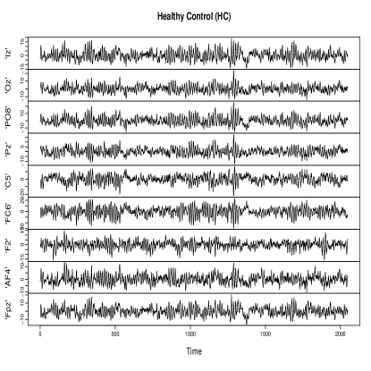
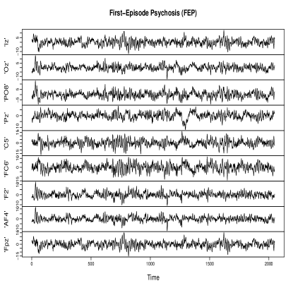
Figure 1: Resting state EEG data from two individuals, a healthy control (HC, left) and a person experiencing a first psychotic episode (FEP, right), from a subset of 9 channels from a 64-channel montage.

Various formulations of the PC problem, alternative methods of imposing sparsity, and convex relaxation of the corresponding optimization problems have inspired a notable volume of research. For iid multivarite data, these methods include diagonal thresh-holding for spiked covariance models (Johnstone and Lu, 2009), regularized regression problem (Zou et al., 2006), low rank matrix approximation with sparsity constraint (Shen and Huang, 2008; Witten et al., 2009), maximizing variability over sparse subspaces (d’Aspremont et al., 2004; Vu et al., 2013), and subspace estimation via orthogonal iteration with sparsification (Ma, 2013; Yuan and Zhang, 2013). Literature on the analysis of sparse PCA for serially dependent data is dearth compared to that for iid multivarite observations. In the time domain, methods for principal subspace estimation under vector autoregressive models were developed by Wang et al. (2013b) and Wang et al. (2013a), which utilizes a two step method of Fantope Projection and Selection (FPS) (Vu et al., 2013) followed by an orthogonal iteration method with sparsification (SOAP). Sparse PCA is even less explored in the frequency domain. To the best of our knowledge, the only previous method for sparse PCA in the frequency domain is a two-step FPS followed by SOAP approach introduced by (Lu et al., 2016).

Being equivalent to finding a sequence of principal subspaces of spectral matrices across frequency, high-dimensional spectral domain PCA has an additional layer of complexity compared to the iid multivaraite case that only considers the principal subspace of a single matrix. This additional complexity presents two types of challenges. First, the ability to consistently estimate a $d$-dimensional principal subspace relies on the first $d$ eigenvalues being sufficiently larger than the remaining eigenvalues, which is often referred to as having a sufficient eigengap. This presents theoretical challenges in a PCA for the entire spectrum across all frequencies since, although there can be a sufficient eigengap at certain frequencies of interest, one is unable to reliably estimate principal subspaces of spectral matrices at frequencies with low power where the eigengap is small. A second challenge emerges with regards to interpretation in applications. The challenge of interpretation is typically addressed by applied researchers by summarizing frequency-domain information by collapsing power within a finite number of pre-defined frequency bands. Although historically derived, pre-defined frequency bands have been shown to be associated with a variety of scientific mechanisms, they are not optimal for parsimoniously summarizing and describing information in any given signal. There has been considerable recent research into methods to address this challenge and to learn frequency bands for a given time series that are optimal in some sense (Bruce et al., 2020; Granados-Garcia et al., 2022; Tuft et al., 2023; Granados-Garcia et al., 2024). However, to the best of our knowledge, there exist no approach to provide a frequency-domain PCA of a stationary time series that is interpretable in that principal components are localized in frequency band.

The concept of localization to improve interpretation has been developed within the context of functional data analysis, where it is often referred to as “interpretable functional data analysis” (James et al., 2009; Chen and Lei, 2015; Zhang et al., 2021). Although functional data analytic methods have been developed for the frequency-domain analysis of replicated time series where several independent time series realizations are observed (Krafty et al., 2011; Krafty, 2015), it should be noted that a different setting and question is considered in this article. This article considers the analysis of a single realization of a multivariate time series, so that we consider PCA in the sense of Brillinger (1964) that involves principal subspaces of spectral matrices as operators on finite complex vector spaces, and not PCA in the functional sense that considers principal subspaces of functional operators over a continuous domain of frequency.

The broad contribution of this paper is the introduction of the first method for conducting interpretable frequency-domain PCA that is both sparse among variables as well as localized in frequency. We formulate a definition for the PCA of multivariate time series that contains a low-rank signal of interest with sparse and localized principal subspaces. We propose an efficient, separable algorithm for estimating the principal subspaces, as well as methods for selecting the sparsity level and localization parameter of the model. The approach estimates the sparse $d$-dimensional principal subspace itself, thus avoiding some of the challenges associated with deflation that is required in approaches to sparse PCA that sequentially estimate one-dimensional subspaces. Moreover, we propose a novel sequential smoothing method that borrows information from lower frequencies to improve estimation and provide interpretability of frequency localization as bands of frequency. Through simulation, we have studied the performance of the proposed algorithms on estimation of the underlying principal subspaces as well as parameter selection. On the theoretical side, we have established the consistency of the estimated principal subspaces in high-dimensions. The proof of consistency follows closely those arguments presented in Wang et al. (2014) and Lu et al. (2016). The difference being two folds. On one hand, the rate of convergence of the distance between the estimated subspaces and the true one is obtained for the smoothed version of the estimated subspaces. On the other hand, the proof technique of Lu et al. (2016) for establishing a concentration inequality, in the sparse operator norm, of their proposed spectral density estimator is adopted to establish a similar concentration inequality for a smoothed estimate.

The remainder of this paper is organized as follows. In Section 2, a formulation of the localized and sparse principal subspaces of the underlying process is described. Section 3 is devoted to estimation procedure, where finding the sparse principal subspaces estimator is described in 3.1, obtaining a localized solution is described in 3.2, and a novel smoothing technique is described in 3.3. Theoretical analysis of the sparse principal component estimator is covered in 3.4. In Section 4, we presented model selection procedures. Section 5 contains the simulation set up and results, and Section 6 contains the result of data analysis. Proof of the theoretical results and tables of the simulation results are available in the supplementary materials.

Notation:

Let $\mathbf{A}=[A_{i,j}]\in\mathbb{C}^{p\times p}$. We denote conjugate transpose of $\mathbf{A}$ by $\mathbf{A}^{\dagger}$ and will use it to represent transpose of a real valued matrix as well. Let $u\in\mathbb{C}^{p}$, the $\ell_{2}$-norm of $u$ is defined as $\|u\|_{2}=\sqrt{u^{\dagger}u}$ and the $\ell_{0}$-norm of $u$ is the number of non-zero elements of $u$. For matrices $\mathbf{A}_{1}$ and $\mathbf{A}_{2}$, we define the inner product as $\langle\mathbf{A}_{1},\mathbf{A}_{2}\rangle=tr(\mathbf{A}_{1}^{\dagger}\mathbf{A}_{2})$ and $\|\mathbf{A}\|_{F}=\sqrt{\langle\mathbf{A},\mathbf{A}\rangle}$, where $tr(\mathbf{A})$ is the trace of $A$. For an index set $\mathcal{I}\subseteq\{1,\dots,p\}$, $\mathbf{A}_{\mathcal{I}}$ denotes the matrix whose $(j,k)$-th entry equals $\mathbf{A}_{j,k}$ if $j,k\in\mathcal{I}$ and zero otherwise, and $|\mathcal{I}|$ denotes the size of $\mathcal{I}$. In this paper, $\|\mathbf{A}\|_{2,0}$ determines the number of non-zero rows of $\mathbf{A}$ and $\|\mathbf{A}\|_{1,1}:=\sum_{i,j}|\mathbf{A}_{i,j}|$. In addition, for Hermitian matrices $\mathbf{A},\mathbf{B}\in\mathbb{C}^{p\times p}$, $\mathbf{A}\preccurlyeq\mathbf{B}$ if and only if $\mathbf{B}-\mathbf{A}$ is positive definite. We denote the real and imaginary parts by $\Re()$ and $\Im()$, respectively, and we define the unit ball in $\mathbb{C}^{p}$ by $\mathbb{S}^{p-1}(\mathbb{C})=\{v\in\mathbb{C}^{p}\mid\|v\|_{2}=1\}$.

2 Localized Sparse Principal Components

2.1 Principal Components in Frequency Domain

Let $\{X(t):t\in\mathbb{Z}\}$ be a $p$-dimensional stationary time series with mean vector $\mathbb{E}[X]=\mu$, auto-covariance matrix $\mathbf{\Gamma}(h)=\mathbb{E}\left\{\left[X(t+h)-\mu_{X}\right]\left[X(t)-\mu\right]^{\dagger}\right\}$, $h=0,\pm 1,\dots$, and spectral density matrix

$$\mathbf{f}(\omega)=(2\pi)^{-1}\sum_{h=-\infty}^{\infty}\mathbf{\Gamma}(h)\exp\{-i\omega h\},\quad-\infty<\omega<\infty,$$

that is continuous as a function of frequency. Consider the decomposition $X(t)=\vartheta(t)+\varepsilon(t),\;t\in\mathbb{Z},$ where $\vartheta$ is the time series that is the closest time series to $X$ in terms of mean square error that can be obtained after compressing then reconstructing $X$ through a $d$-dimensional linear filter. Formally, $\vartheta$ is defined by the $d\times p$ filter $\{\mathbf{b}(h)\}$ and the $p\times d$ filter $\{\mathbf{c}(h)\}$ such that $\vartheta(t)=\mu_{\vartheta}+\sum_{h}\mathbf{c}(t-h)\zeta(h)$ and $\zeta(t)=\sum_{h}\mathbf{b}(t-h)X(h)$ minimizes

$$\mathbb{E}\left\{\left[X(t)-\vartheta(t)\right]^{\dagger}\left[X(t)-\vartheta(t)\right]\right\}$$ (1)

over all possible $d\times p$ and $p\times d$ filters.

Let $\mathbf{B}(\omega)=\sum_{h}\mathbf{b}(h)\exp\{i\omega h\}$ and $\mathbf{C}(\omega)=\sum_{h}\mathbf{c}(h)\exp\{i\omega h\}$ be the corresponding transfer functions. The next theorem, presented in Brillinger (2001), identifies the optimal transfer functions that minimizes Equation (1).

Theorem 1.

Let $\{X(t)\}$ be a $p$-dimensional weakly stationary time series with mean vector $\mu$, an absolutely summable autocovariance function $\mathbf{\Gamma}(h)$, and spectral density matrix $\mathbf{f}(\omega),-\infty<\omega<\infty$. Then the $\mu_{\vartheta},\{\mathbf{b}(h)\}$, and $\{\mathbf{c}(h)\}$ that minimizes (1) are given by $\mu_{\vartheta}=\mu-\left[\sum_{h}\mathbf{c}(h)\right]\left[\sum_{h}\mathbf{b}(h)\right]\mu$, $\mathbf{b}(h)=(2\pi)^{-1}\int_{0}^{2\pi}\mathbf{B}(\alpha)\exp\{ih\alpha\}\;d\alpha$, and $\mathbf{c}(h)=(2\pi)^{-1}\int_{0}^{2\pi}\mathbf{C}(\alpha)\exp\{ih\alpha\}\;d\alpha,$ where $\mathbf{C}(\omega)=[U_{1}(\omega)\dots U_{d}(\omega)]$, $\mathbf{B}(\omega)=\mathbf{C}^{\dagger}(\omega)$, and $U_{j}(\omega)$ is the $j$-th eigenvector of $\mathbf{f}(\omega),j=1,\dots,p$. In addition, if $\lambda_{j}(\omega)$ denotes the corresponding eigenvalue, $j=1,\dots,p$, then the minimum obtained is $\int_{0}^{2\pi}\sum_{j>d}\lambda_{j}(\alpha)\;d\alpha$.

Note that if we denote $\mathbf{A}(\omega)=\mathbf{C}(\omega)\mathbf{B}(\omega)$, then

$$\mathbb{E}\left\{\left[X(t)-\vartheta(t)\right]^{\dagger}\left[X(t)-\vartheta(t)\right]\right\} =\int_{0}^{2\pi}\text{tr}\left\{\left[I-\mathbf{A}\left(\omega\right)\right]\mathbf{f}(\omega)\left[I-\mathbf{A}(\omega)\right]^{\dagger}\right\}\;d(\omega)$$

$$\mathbf{A}(\omega) =U_{1}(\omega)U_{1}(\omega)^{\dagger}+\dots+U_{d}(\omega)U_{d}(\omega)^{\dagger}.$$

In other words, for each $\omega\in[0,1)$, $\mathbf{A}(\omega)$ is a rank $d$ projection matrix. This indicates that the solution to the minimization problem

$$\min_{\mathbf{A}\in\mathcal{G}_{d}}\int_{0}^{2\pi}\text{tr}\left\{\left[I-\mathbf{A}(\omega)\right]\mathbf{f}(\omega)\left[I-\mathbf{A}(\omega)\right]^{\dagger}\right\}\;d(\omega),$$ (2)

where $\mathcal{G}_{d}$ is the space of rank-$d$ projection matrices, is equivalent to the solution to the maximization problem

$$\max_{A\in\mathcal{G}_{d}}\int_{0}^{2\pi}\text{tr}\left[\mathbf{f}(\omega)\mathbf{A}(\omega)\right]\;d(\omega).$$ (3)

The focus of this article is the interpretation and estimation of the principal subspace spanned by the orthogonal directions $U_{j}\left(\omega\right)$, considered with reference to the eigenvalues $\lambda_{j}\left(\omega\right)$. It should be noted that the power spectrum of $\vartheta$ can be represented as

$$\mathbf{f}_{\vartheta}\left(\omega\right)=\sum_{j=1}^{d}\lambda_{j}\left(\omega\right)U_{j}\left(\omega\right)U_{j}\left(\omega\right)^{\dagger}.$$

The principal time series $\zeta_{j}\left(t\right)$, $j=1,\dots,d$, are uncorrelated time series with power spectra $\lambda_{j}\left(\omega\right)$ that represent parsimonious underlying latent mechanisms that account for most of the information in $X\left(t\right)$. The orthogonal directions $U_{j}\left(\omega\right)$ describe how these latent time series relate to and can be interpreted from the perspective of the $p$-dimensional space. For example, in our analysis of the EEG data that is presented in Section 6, $U_{j}$ and $\lambda_{j}$ are dominated by information within a subset of the $\delta$ frequencies between 0.5 - 4 Hz, which has been shown to be most prominent during times of and can be used to electrophysiologically quantify rest, and within a subset of the $\theta$ frequencies between 4 - 7 Hz, which has been shown to be associated with attention control. The principal time series $\zeta_{j}$ represent uncorrelated relative expression of these two mechanisms, and the principal directions $U_{j}$ indicate how these mechanisms are expressed in each location of the brain.

2.2 Sparsity

This article is concerned with PCA where principal subspaces are sparse in variates. This assumption is essential both to make estimation tractable in the high-dimensional setting, as well as for interpretation. For example, in our motivating application, we desire a parsimonious interpretation where a component represent power in only certain regions of the brain by estimating principal subspaces that are sparse in the following sense.

Definition 2 (Subspace Sparsity).

Let $\mathcal{U}$ be a $d$-dimensional subspace of $\mathbb{C}^{p}$ and $\mathbb{U}$ be the set of $p\times d$ orthonormal matrices whose column span $\mathcal{U}$. Let $\mathbf{\Pi}=\mathbf{U}\mathbf{U}^{\dagger},\mathbf{U}\in\mathbb{U}$ be the unique (orthogonal) projection matrix onto the subspace $\mathcal{U}$. We define the sparsity level of $\mathcal{U}$ as $s=\left|\mbox{supp}\left[\mbox{diag}\left(\mathbf{\Pi}\right)\right]\right|$.

We desire a principal component analysis under the assumption that the principal subspace $\mathbf{A}\left(\omega\right)$ that is spanned by $U_{1}\left(\omega\right),\dots,U_{d}\left(\omega\right)$ is sparse with sparsity level $s^{*}$.

2.3 Frequency Localization

In addition to sparsity, we also desire a PCA that is localize in the frequency domain in that only the most relevant frequencies are retained. Frequency localization is important for two reasons. In terms of estimation, the ability to consistently estimate the $d$-dimensional principal subspace of a matrix depends on the difference between the $d$th and $d+1$st eigenvalues. In many applications, including our motivating EEG example where there is low signal at higher frequencies, this eigengap is not sufficiently large for spectral matrices at many frequencies. In terms of interpretation and applications, we desire a parsimonious decomposition of information in that principal components can be interpretable as having support withing certain ranges or bands of frequency. This desire also mitigates the issues caused by the inability to consistently estimate principal subspaces at frequencies with insufficient eigengaps as said information is not of practical interest. Formally, we desire a frequency localization procedure that identifies frequencies with sufficient power by finding $\Omega\subset\left[0,2\pi\right)$ such that the power of $X$ at frequency $\omega$ that is accounted for by $\vartheta$, or $\sum_{j=1}^{d}\lambda_{j}(\omega)$, is greater than some threshold for all $\omega\in\Omega$. Although this threshold can be selected either subjectively or based on existing scientific knowledge, in Section 4 we present a data driven procedure for selecting this threshold relative to the variance of the remainder $\text{Var}\left[\epsilon\left(t\right)\right]=\sum_{j>d}\int\lambda_{j}(\omega)d\omega$.

2.4 Optimization

Our estimation of a sparse localized PCA begins by considering a frequency domain transformation of the time series data to obtain an asymptotically unbiased estimate of the spectral matrices $\mathbf{f}_{\Psi}\left(\omega\right)$ that can depend on some parameters $\Psi$. This estimator includes common frequency domain transformations of $X(t)$ such as the periodogram, tapered periodogram, multitaper estimate, and appropriately smoothed periodogram. In Section 3.3, we propose a novel smoothed estimate that enables for efficient sequential implementation by shrinking the $d$-dimensional principal subspace of $\mathbf{f}\left(\omega_{\ell+1}\right)$ towards the previously estimated principal subspace at frequency $\omega_{\ell}$. This smoothing step, which indirectly regularizes the spectral matrix itself via directly regularizing its principal subspace, is important for two reasons. First, it provides stability by sharing information across frequencies. Second, it assures that the frequency localization provides measures that are interpreted as power within continuous bands of frequency.

The equivalence between (2) and (3) enables us to formulate and estimate the localized and sparse principal components. First, in order to obtain a sparse solution to the optimization problem (3), we can add the $\ell_{0}$ penalty term for each frequency component. Second, to obtain a localized solution, we propose to discretize the objective function in (3) and add a shrinkage parameter for each frequency. Combining the two steps, and given $\mathbf{f}_{\Psi}\left(\omega\right)$, we propose to estimate the sparse and localized principal components through solving the following optimization problem.

$$\begin{split}\underset{\ell=1,\dots,n/2}{\underset{\beta_{\ell},V(\omega_{\ell})}{\mbox{maximize}}}\;&\left\{\sum_{\ell=1}^{n/2}\beta_{\ell}\text{tr}\left[\mathbf{f}_{\Psi}(\omega_{\ell})\mathbf{V}(\omega_{\ell})\mathbf{V}(\omega_{\ell})^{\dagger}\right]\right\}\\ \mbox{subject to: }&\;\;\mathbf{V}(\omega_{\ell})\mbox{ orthonormal, }\|\mathbf{V}(\omega_{\ell})\|_{2,0}\leq s^{*}\mbox{ and }\\ &\;\sum_{j=1}^{n/2}\beta_{\ell}\leq\eta\;\mbox{ and }0\leq\beta_{\ell}\leq 1,\ell=1,\dots,n/2.\end{split}$$ (4)

3 Estimation procedure

First observe that the optimization problem in (4) is separable, i.e. we can first optimize with respect to $\mathbf{V}(\omega_{\ell}),\ell=1,\dots,n/2$ and then with respect to $\beta_{\ell},\ell=1,\dots,n/2$. More precisely, we can write the problem as

$$\begin{split}\underset{\sum_{j=1}^{n/2}\beta_{\ell}\leq\eta\;\mbox{ and }0\leq\beta_{\ell}\leq 1,\ell=1,\dots,n/2}{\underset{\beta_{1},\dots,\beta_{n/2}}{\mbox{maximize}}}\;&\left\{\sum_{\ell=1}^{n/2}\beta_{\ell}\underset{\ell=1,\dots,n/2}{\underset{\mathbf{V}(\omega_{\ell})}{\max}}\;\text{tr}\left[\mathbf{f}_{\Psi}(\omega_{\ell})\mathbf{V}(\omega_{\ell})\mathbf{V}(\omega_{\ell})^{\dagger}\right]\right\}\\ \mbox{subject to: }&\;\;\mathbf{V}(\omega_{\ell})\mbox{ orthonormal, }\|\mathbf{V}(\omega_{\ell})\|_{2,0}\leq s^{*}.\end{split}$$ (5)

Note that the later optimization problem is a constraint linear programming problem with increasing objective function, as a function of $\beta_{\ell},\ell=1,\dots,n/2$. For this reason, when $\eta\in\mathbb{N}$, the solution falls on the corners of the constraint set (Proposition (3.1)). This indicates that the estimated $\beta_{\ell},\ell=1,\dots,n/2$ are either zero or one; in other words, the optimization problem selects the first $\eta$ frequency components with highest objective function. On the other hand, the former optimization problem is also separable and each problem is a sparse principal component analysis of the spectral density matrix at a fundamental frequency. We consider solving the former problem through the two step procedure of Fantope projection and selection (FPS) followed by sparse orthogonal iterated pursuit (SOAP) proposed by Wang et al. (2014).

3.1 Solution of the Sparse Principal Components

Although the solution to

$$\underset{\mathbf{V}(\omega_{\ell})}{\max}\;\text{tr}\left[\mathbf{f}_{\Psi}(\omega_{\ell})\mathbf{V}(\omega_{\ell})\mathbf{V}(\omega_{\ell})^{\dagger}\right],\quad\mbox{s.t. }\mathbf{V}(\omega_{\ell})\mbox{ orthonormal, }\|\mathbf{V}(\omega_{\ell})\|_{2,0}\leq s^{*},$$ (6)

for each $\ell=1,\dots,n/2$ can attain the optimal statistical rate of convergence (Vu and Lei, 2012, 2013), it is NP-hard to compute (Moghaddam et al., 2005). Extensive research has been done to design a computationally feasible algorithm that enjoys optimal statistical convergence rate, a review of which can be found in Section D of Zou and Xue (2018). In this article, we adopted the two step algorithm proposed by Wang et al. (2014) that applies to the non-spiked covariance models, and non-Gaussian as well as dependent data.

The optimization problem (6) can be solved directly by the orthogonal iteration algorithm (Golub and Van Loan, 2013) combined with a sparsification step. In addition, to ensure the solution attains optimal statistical rate of convergence, the initial value should fall within an appropriate distance from the solution. The initial estimate is obtained by applying the Fantope projection and selection (FPS) method that solves a convex relaxation of the problem (6). The two steps of (relaxed step) FPS followed by (tightened step) SOAP are explained below.

We first introduce the FPS algorithm for estimating the sparse PCs of a real matrix $\mathbf{\Sigma}$, where we maximize $\text{tr}\left[\mathbf{\Sigma}\mathbf{V}\mathbf{V}^{\dagger}\right]$ subject to $\mathbf{V}$ being orthonormal and $\|\mathbf{V}\|_{2,0}\leq s^{*}$. We then extend it so that it can estimate the sparse principal subspace of a complex valued spectral density matrix. Note that we can relax the constraint set of (6) to obtain a convex relaxation of the problem. To do so, let $\mathbf{\Pi}=VV^{T}$ and note that since $\mathbf{V}$ is an orthonormal matrix, $\mathbf{\Pi}$ is the projection matrix onto a $d$-dimensional subspace of $\mathbb{R}^{p}$ (in the real case). In addition, we know that $\mathbf{\Pi}$ has exactly two eigenvalues, $1$ with multiplicity $d$ and $0$ with multiplicity $p-d$. Such constraint on eigenvalues of $\mathbf{\Pi}$ can be relaxed to $\text{tr}\left(\mathbf{\Pi}\right)=d$ and $0\preccurlyeq\mathbf{\Pi}\preccurlyeq\mathbb{I}_{p}$. In addition, we relax the constraint $\|\mathbf{\Pi}\|_{2,0}\leq s^{*}$ to $\|\mathbf{\Pi}\|_{1,1}\leq s^{*}$. Note that the constraint set $\{\|\mathbf{V}\|_{2,0}\leq s^{*}\}$ is not convex, while the set $\mathcal{A}=\{\mathbf{\Pi}:\mathbf{\Pi}\in\mathbb{R}^{p\times p},\text{tr}({\mathbf{\Pi}})=d,0\preccurlyeq\mathbf{\Pi}\preccurlyeq\mathbb{I}_{p}\}$ is convex.

The relaxed convex optimization problem can be equivalently expresses as

$$\mbox{minimize }\{\text{tr}({\mathbf{\Sigma}}\;\mathbf{\Pi})+\rho\|\mathbf{\Phi}\|_{1,1}\;|\;\mathbf{\Pi}=\mathbf{\Phi},\mathbf{\Pi}\in\mathcal{A},\mathbf{\Phi}\in\mathbb{R}^{p\times p}\},$$ (7)

with the Lagrangian

$$\mathcal{L}(\mathbf{\Pi},\mathbf{\Phi},\mathbf{\Theta})=\text{tr}({\mathbf{\Sigma}}\;\mathbf{\Pi})+\rho\|\mathbf{\Phi}\|_{1,1}-\text{tr}\left[{\mathbf{\Theta}\left(\mathbf{\Pi}-\mathbf{\Theta}\right)}\right],\quad\mathbf{\Pi}\in\mathcal{A},\mathbf{\Phi}\in\mathbb{R}^{p\times p},\mathbf{\Theta}\in\mathbb{R}^{p\times p},$$ (8)

and be solved by the alternating direction of multiplier (ADMM), which iteratively minimizes the augmented Lagrangian,

$$\mathcal{L}(\mathbf{\Pi},\mathbf{\Phi},\mathbf{\Theta})+\beta/2\|\mathbf{\Pi}-\mathbf{\Phi}\|_{F}^{2}$$ (9)

with respect to $\mathbf{\Pi}$ and $\mathbf{\Phi}$ and updating the dual variable $\mathbf{\Theta}$. We only need to iterate the algorithm enough so that the calculated $\mathbf{\Pi}$ at iteration $T$, $\mathbf{\Pi}^{(T)}$, falls within the basin of attraction of the SOAP algorithm. A detailed description of the ADMM step can be found in Appendix A. Then, the top $d$ leading eigenvectors of $\mathbf{\Pi}^{(T)}$ are used as the initial value in the SOAP algorithm.

To apply the FPS algorithm to complex valued metrics we invoke to Lemma (B.4.3) from the Appendix that describes the isomorphism between complex matrices and real matrices. In particular, let

$$\mathbf{f}^{(R)}(\omega_{\ell}):=\begin{bmatrix}\Re{\left\{\mathbf{f}(\omega_{\ell})\right\}}&\Im{\left\{\mathbf{f}(\omega_{\ell})\right\}}\\ -\Im{\left\{\mathbf{f}(\omega_{\ell})\right\}}&\Re{\left\{\mathbf{f}(\omega_{\ell})\right\}}\end{bmatrix}\,\mbox{ and }\,{\mathbf{f}}^{(R)}_{\Psi}(\omega_{\ell}):=\begin{bmatrix}\Re{\left\{{\mathbf{f}}_{\Psi}(\omega_{\ell})\right\}}&\Im{\left\{{\mathbf{f}}_{\Psi}(\omega_{\ell})\right\}}\\ -\Im{\left\{{\mathbf{f}}_{\Psi}(\omega_{\ell})\right\}}&\Re{\left\{{\mathbf{f}}_{\Psi}(\omega_{\ell})\right\}}\end{bmatrix}.$$ (10)

If the eigenvalues and corresponding eigenvectors of $\mathbf{f}(\omega_{\ell})$ are $\lambda_{j}(\omega_{\ell})$ and $u_{j}(\omega_{\ell}),j=1,\dots,p$, then the $\left[2\left(j+1\right)+1\right]$st and $\left[2\left(j+1\right)+2\right]$st eigenvalues and corresponding eigenvectors of $\mathbf{f}^{(R)}(\omega_{\ell})$ are

$$\lambda_{j}(\omega_{\ell}),\,\begin{bmatrix}\Re{\left\{u_{j}(\omega_{\ell})\right\}}\\ \Im{\left\{u_{j}(\omega_{\ell})\right\}}\end{bmatrix}\mbox{ and }\lambda_{j}(\omega_{\ell}),\,\begin{bmatrix}-\Im{\left\{u_{j}(\omega_{\ell})\right\}}\\ \Re{\left\{u_{j}(\omega_{\ell})\right\}}\end{bmatrix}.$$

Hence, we propose to apply the FPS algorithm to $\mathbf{f}_{\Psi}^{(R)}(\omega_{\ell})$ and estimate the $2d$-dimensional principal subspace of $\mathbf{f}_{\Psi}^{(R)}(\omega_{\ell})$ to obtain the initial estimate of $d$ leading eigenvectors of $\mathbf{f}(\omega_{\ell})$. As will be shown in Theorem (3), part (I), the estimated subspace obtained in this manner will be consistent.

In the Tightened step, the orthogonal iteration method is followed by a truncation step to enforce row-sparsity and further followed by taking another re-normalization step to enforce orthogonality. More precisely, at the $t$-th iteration of the algorithm the following operations are performed

• Orthogonal iteration: $\tilde{\mathbf{V}}^{(t+1)}\leftarrow{\mathbf{f}}_{\Psi}(\omega)\mathbf{U}^{(t)};\;\mathbf{V}^{(t+1)},\mathsf{\mathbf{R}}_{1}^{(t+1)}\leftarrow\mbox{QR}(\tilde{\mathbf{V}}^{(t+1)})$

• Truncation/re-normalization: $\tilde{\mathbf{U}}^{(t+1)}\leftarrow\mbox{Truncate}(\mathbf{V}^{(t+1)},\hat{s});\;\mathbf{U}^{(t+1)},\mathsf{\mathbf{R}}_{2}^{(t+1)}\leftarrow\mbox{QR}(\tilde{\mathbf{U}})^{(t+1)}$

where columns of $\mathbf{U}^{(t)}$ contain the estimated first $d$ eigenvectors of $\mathbf{f}(\omega)$ and the truncation operator sets the $p-\hat{s}$ rows with the smallest modulus to zero.

3.2 Solution of the Linear Programming Problem

Let $\hat{\mathbf{V}}(\omega_{\ell}),\ell=1,\dots,n/2$ be a solution to

$$\underset{\mathbf{V}(\omega_{\ell})}{\max}\;\text{tr}\{[\mathbf{f}_{\Psi}(\omega_{\ell})]\mathbf{V}(\omega_{\ell})\mathbf{V}(\omega_{\ell})^{\dagger}\},\quad\mbox{s.t. }\mathbf{V}(\omega_{\ell})\mbox{ orthonormal, }\|\mathbf{V}(\omega_{\ell})\|_{2,0}\leq s^{*}.$$

Since $\mathbf{f}_{\Psi}(\omega_{\ell}),\ell=1,\dots,n/2$ are positive definite, $h_{\ell}:=\text{tr}\left[\mathbf{f}_{\Psi}(\omega_{\ell})\hat{\mathbf{V}}(\omega_{\ell})\hat{\mathbf{V}}(\omega_{\ell})^{\dagger}\right]>0$. Thus, we can write (5) as

$$\underset{\sum_{\ell=1}^{n/2}\beta_{\ell}\leq\eta\;\mbox{ and }0\leq\beta_{\ell}\leq 1,\ell=1,\dots,n/2}{\underset{\beta_{1},\dots,\beta_{n/2}}{\mbox{maximize}}}\;\left\{\sum_{\ell=1}^{n/2}\beta_{\ell}h_{\ell}\right\}.$$ (11)

Note that, since $h_{\ell}>0,\ell=1,\dots,n/2$, the objective function is monotonically increasing in $\beta_{\ell},\ell=1,\dots,n/2$ and therefore attains its maximum on the boundary of the constraint set. We claim that the algorithm selects the $\eta$ largest $h_{j}$’s and set the coefficients of the $n/2-\eta$ smallest $h_{j}$‘s to zero.

Proposition 3.1.

Let $\eta\in\mathbb{N}$, $\eta<K$ for some $K\in\mathbb{N}$, and $h_{1},\dots,h_{K}\in\mathbb{R}^{+}$. In addition, let $h_{(1)}\geq\dots\geq h_{(K)}$ be the sorted $h_{j}^{\prime}s$ in decreasing order and $\beta_{(1)},\dots,\beta_{(K)}$ be the corresponding coefficients in (11). Then

$$\underset{\sum_{\ell=1}^{K}\beta_{\ell}\leq\eta\;\mbox{ and }0\leq\beta_{\ell}\leq 1,\ell=1,\dots,K}{\underset{\beta_{1},\dots,\beta_{K}}{\mbox{maximum}}}\;\left\{\sum_{\ell=1}^{K}\beta_{\ell}h_{\ell}\right\}.$$ (12)

is attained at $\beta_{(1)}=\dots=\beta_{(\eta)}=1,\beta_{(\eta+1)}=\dots=\beta_{(K)}=0$

3.3 Smoothing by Borrowing Information from Previous Frequency

The previously developed methodology is applicable for any common quadratic transformation of the times series to obtain a asymptotically unbiased estimator of spectral matrices $\mathbf{f}_{M}(\omega)$, where $M$ is some parameter. This includes frequency-domain transformations such as the periodogram, for which $M$ is trivial, multitaper estimators, for which $M$ is the number of tapers, kernel estimator, for which $M$ is the bandwidth, and the truncated periodogram that will be considered when establishing theoretical properties

$$\mathbf{f}_{M}(\omega)=\sum_{t=-M}^{M}\hat{\mathbf{R}}_{t}\exp\{-2\pi i\omega t\},$$ (13)

and $\hat{\mathbf{R}}_{t}=\frac{1}{n}\sum_{k=1}^{n-t}X(k+t)X(t)^{\dagger}$.

The explicit sharing of information across frequency principle subspaces is important for improving stability of principle subspace estimation, especially in frequencies with low signal. It is also important for assuring that frequency localization produces frequency bands that are essential for interpretation. We introduce a novel approach to sharing information to directly regularize on our object of interest, the principle subspace, and to do so interactively to shrink towards the previous principle subspace, which makes for fast computation. The approach considers incorporating smoothness through $\mathbf{f}_{\Psi}$ considered in the previous sections, $\Psi=\left(M,\theta\right)$, where $\theta$ is a parameter that controls smoothness through the dependence on the estimate at the previous frequency. This separation of the incorporation of smoothness from regulation on sparsity or localization enables efficient computation.

Given $\mathbf{f}_{M}(\omega_{\ell})$, we propose a smoothing method that borrows information from the estimated principal subspace obtained from the previous frequency component. More precisely, suppose $\hat{\mathbf{\Pi}}^{\Psi}_{\ell}$ is the $d$-dimensional principal subspace of $\mathbf{f}(\omega_{\ell}),\;\ell=1,\dots,n/2$. One can obtain the projection of the left and right eigenvectors of $\mathbf{f}_{M}(\omega_{\ell+1})$ on the estimated $d$-dimensional principal subspace of $\mathbf{f}(\omega_{\ell})$ by $\hat{\mathbf{\Pi}}_{\ell}^{\Psi}\mathbf{f}_{M}(\omega_{\ell+1})\hat{\mathbf{\Pi}}_{\ell}^{\Psi}$. Since the spectral density matrices are continuous as a function of frequency, we propose to combine information at frequency $\omega_{\ell}$ and $\omega_{\ell+1}$ by estimating $\mathbf{\Pi}_{\ell+1}$, denoted by $\hat{\mathbf{\Pi}}_{\ell+1}^{\Psi}$, by applying the LSPCA Algorithm to

$$\mathbf{f}_{\Psi}(\omega_{\ell+1}):=(1-\theta)\mathbf{f}_{M}(\omega_{\ell+1})+\theta\;\hat{\mathbf{\Pi}}_{\ell}^{\Psi}\mathbf{f}_{M}(\omega_{\ell+1})\hat{\mathbf{\Pi}}_{\ell}^{\Psi}.$$ (14)

3.4 Theoretical Analysis

To investigate theoretical properties, we first introduce the notion of distance between subspaces, in addition to several key quantities which will be used in the theoretical analysis, then we present the rate of convergence of the the estimated localized sparse principal components.

• Subspace distance: Let $\mathcal{U}$ and $\mathcal{U}^{\prime}$ be two $d$-dimentional subspaces of $\mathbb{C}^{p}$. Denote the projection matrices onto them by $\mathbf{\Pi}$ and $\mathbf{\Pi}^{\prime}$, respectively. We define and denote the distance between $\mathcal{U}$ and $\mathcal{U}^{\prime}$ by $\mathcal{D}(\mathcal{U},\mathcal{U}^{\prime})=\|\mathbf{\Pi}-\mathbf{\Pi}^{\prime}\|_{F}$.

• Principal subspace notations: Let $\mathcal{U}^{*}_{\ell}$ be the $d$-dimensional principal subspace of $\mathbf{f}(\omega_{\ell})$ for each fundamental frequency $\omega_{\ell}=\ell/n,\ell=2,\dots,n/2$ and $\mathcal{U}^{(t)}(\omega_{1})$ be the $d$-dimensional subspace spanned by the top $d$ eigenvectors of $\bar{\mathbf{\Pi}}^{(t)}$ obtained at the $t$-th iteration of the ADMM algorithm presented in the Appendix A.

• Minimum number of iterations and data points: Let $\gamma=\sup_{\omega\in[0,1]}\frac{3\lambda_{d+1}(\omega)+\lambda_{d}(\omega)}{\lambda_{d+1}(\omega)+3\lambda_{d}(\omega)}$ and $R=\min\left\{\sqrt{\frac{d\gamma(1-\gamma^{1/2})}{2}},\frac{\sqrt{2\gamma}}{4}\right\}$. The minimum number of iterations of the ADMM, $T_{min}$, the SOAP, $\tilde{T}_{min}$, and the minimum data points, $n_{min}$, are

  $$T_{\min}=\left\lceil\frac{\zeta_{1}^{2}}{(R-\zeta_{2})^{2}}\right\rceil;\;\tilde{T}_{\min}=\left\lceil\frac{4\log(R/\xi)}{\log(1/\gamma)}\right\rceil;\;n_{\min}=C\frac{(s^{*})\log(p)}{R^{2}}\left(\frac{\lambda_{1}(\omega_{1})}{\lambda_{d}(\omega_{1})-\lambda_{d+1}(\omega_{1})}\right)^{2},$$ (15)

  where $\zeta_{1}=\frac{\tilde{C}^{\prime}\lambda_{1}(\omega_{1})}{\lambda_{d}(\omega_{1})-\lambda_{d+1}(\omega_{1})}.s^{*}\sqrt{\frac{\log(p)}{n}}$, and $\zeta_{2}=\frac{\tilde{C}^{\prime\prime}\sqrt{M(n)\lambda_{1}(\omega_{1})}}{\sqrt{\lambda_{d}(\omega_{1})-\lambda_{d+1}(\omega_{1})}}\left(\frac{d.p^{2}\log(p)}{n}\right)^{1/4}\frac{1}{\sqrt{t}}$.

Theorem 3.

Let $\{X(t):t=1,\dots,n\}$ be a realization of a weakly stationary time series that follows $\mathcal{M}_{d}(f,d,s^{*})$, as defined in Appendix B, with $n>n_{min}$ and ${f}_{M}(\omega_{1})$ be as defined in (13). Let the regularization parameter in (7) be $\varrho=C\lambda_{1}(\omega_{1})\sqrt{\log(p)/n}$ for a sufficiently large constant $C$, and the penalty parameter $\beta$ in (9) be $\beta=\sqrt{2}p.\varrho/\sqrt{d}$.

• The iterative sequence of $d$-dimensional subspace $\{\mathcal{U}^{(t)}(\omega_{1})\}_{t=1}^{T}$ satisfies

  $$\footnotesize\mathcal{D}(\mathcal{U}^{(t)}(\omega_{1}),\mathcal{U}^{*}(\omega_{1}))\leq\frac{\tilde{\tilde{C}}^{\prime}\lambda_{1}(\omega_{1})}{\lambda_{d}(\omega_{1})-\lambda_{d+1}(\omega_{1})}.s^{*}\sqrt{\frac{\log(p)}{n}}+\frac{\tilde{\tilde{C}}^{\prime\prime}\sqrt{M(n)\lambda_{1}(\omega_{1})}}{\sqrt{\lambda_{d}(\omega_{1})-\lambda_{d+1}(\omega_{1})}}\left(\frac{d.p^{2}\log(p)}{n}\right)^{1/4}\frac{1}{\sqrt{t}}$$ (16)

  with high probability, where $\tilde{\tilde{C}}^{\prime}$ and $\tilde{\tilde{C}}^{\prime\prime}$ are constants.

• When $\theta<\max_{\ell}\frac{\lambda_{d}(\omega_{\ell+1})-\|\mathbf{f}_{M}(\omega_{\ell+1})-\mathbf{f}(\omega_{\ell+1})\|_{op,|\mathcal{I}|}}{2\lambda_{1}(\omega_{\ell+1})\left[\mathcal{D}(\mathcal{U}^{*}_{\ell},\mathcal{U}^{*}_{\ell+1})+\alpha\right]+\lambda_{d+1}(\omega_{\ell+1})},$ by taking the sparsity parameter $\hat{s}$ in Algorithm SOAP such that $\hat{s}=C\max\left\{\left[\frac{4d}{(\gamma^{-1/2}-1)^{2}}\right],1\right\}s^{*}$ for some integer constant $C\geq 1$, $T\geq T_{min}$ iterations in Algorithm ADMM, and then $\tilde{T}\geq\tilde{T}_{min}$ iterations of Algorithm SOAP, the final estimator $\hat{\mathcal{U}}_{\ell}=\mathcal{U}^{(T+\tilde{T})}_{\ell}$ satisfies

  $$\mathcal{D}(\mathcal{U}^{*}_{\ell},\hat{\mathcal{U}}_{\ell})\leq C^{\prime\prime\prime}\frac{\gamma^{1/2}}{1-\gamma^{1/4}}\Delta(2\hat{s})$$

  with high probability, for all $\ell=1,2,\dots,n/2$, where

  $$\footnotesize\Delta(s):=\sup_{\omega_{\ell}}\frac{\sqrt{2d}\left[\left(\exp(-c_{0}M(n))\vee M(n)\sqrt{\frac{s^{*}\log(p)}{n}}\right)+2\theta\lambda_{1}(\omega_{\ell+1})\left[\mathcal{D}(\mathcal{U}^{*}_{\ell},\mathcal{U}^{*}_{\ell+1})+\alpha\right]+\theta\lambda_{d+1}(\omega_{\ell+1})\right]}{\frac{1}{2}\left[\lambda_{d}(\omega_{\ell+1})-(1-\theta)\lambda_{d+1}(\omega_{\ell+1})\right]-2\theta\lambda_{1}(\omega_{\ell+1})\alpha},$$ (17)

  $\alpha=\sup_{\omega_{\ell}}\frac{c_{1}\sqrt{2d}}{\lambda_{d}(\omega_{\ell})-\lambda_{d+1}(\omega_{\ell})}\left(\exp(-c_{0}M(n)\vee M(n)\sqrt{\frac{s^{*}\log(p)}{n}}\right),$ and $\mathcal{U}^{(T+\tilde{T})}_{\ell}$ be the space spanned by the columns of the estimator obtained from the Algorithm LSPCA.

4 Model Selection

In this section we address selection of four parameters: $d$, the dimension of the principal subspaces, $\hat{s}$ the sparsity parameter in Algorithm SOAP, $\eta$ the localization parameter, and $\theta$ the smoothing parameter. Given the complex nature of the problem that makes the empirical joint selection of the parameters infeasible, we propose the selection of each parameter individually. Below we present an outline of the procedure; a detailed description is provided in the Supplementary materials.

• Dimension of Principal Subspaces: We follow the general approach of determining the dimension of principal subspace by inspecting the scree plot or equivalently by the plot of the proportion of variance explained.

• Localization Parameter: We propose to use information criteria based on the log-Whittle likelihood. More precisely, for each $\eta$, let $\check{L}_{\kappa}=\{\ell_{(1)},\dots,\ell_{(\kappa)}\}\in\check{L}:=\{1,2,\dots,n/2\}$. The log-Whittle likelihood is estimated by

  $$\log(\mathcal{L})=-\sum_{\ell=1}^{n/2}\{p\log{\pi}+\log{|\hat{\mathbf{G}}_{\ell}|}+[d_{X}(\omega_{\ell})][\hat{\mathbf{G}}_{\ell}]^{-1}[d_{X}(\omega_{\ell})]^{\dagger}\},$$

  where $\hat{\mathbf{G}}_{\ell}=\mathbb{I}\{\ell\in\check{L}_{\kappa}\}\hat{\mathbf{f}}^{(d)}_{\vartheta}(\omega_{\ell})+\hat{\Sigma}$, $\hat{\mathbf{f}}_{\vartheta}(\omega_{\ell})={\mathbf{f}}_{\Psi}(\omega_{\ell})\hat{U}_{1}(\omega_{\ell})\hat{U}_{1}(\omega_{\ell})^{\dagger}+\dots+{\mathbf{f}}_{\Psi}(\omega_{\ell})\hat{U}_{d}(\omega_{\ell})\hat{U}_{d}(\omega_{\ell})^{\dagger}$, $\hat{U}_{j}(\omega_{\ell})$ are obteined from the LSPCA algorithm, $\hat{\mathbf{\Sigma}}=\sum_{\ell\in\check{L}/\check{L}_{\kappa}}d_{X}(\omega_{\ell})d_{X}(\omega_{\ell})^{\dagger}/\left(|\check{L}|-|\check{L}_{\kappa}|\right)$, and $d_{X}(\omega_{\ell})$ is the discrete Fourier transform of the data at $\omega_{\ell}$. We use to the $\hat{\mathbf{G}}_{\ell}$ to define standard information criteria for $\eta$ including $AIC=-2\log(\mathcal{L})+2|L_{K}|$, $AICc=-2\log(\mathcal{L})+2|L_{K}|+\frac{2|L_{K}|^{2}+2|L_{K}|}{n-|L_{K}|-1}$, and $BIC=-2\log(\mathcal{L})+\log(n)|L_{K}|$. The localization parameter $\eta$ is selected to minimizing an information criteria.

• Sparsity Parameter: For selecting the sparsity level of the underlying process, we propose to use $k$-folds cross validation, with the Mahalanobis distance to evaluate the performance of fitted model in the validation step.

• Smoothing parameter: We use $k$-folds cross validation similar to the sparsity parameter selection.

5 Simulation Results

5.1 Sparsity Parameter Selection

To illustrate the performance of the LSPCA algorithm, effect of smoothing, and performance of the parameter selection procedures, we examined two settings each for 4 combinations of time series length and dimension: $(p=64,n=2048),(p=64,n=4096),(p=128,n=2048)$, and $(p=128,n=4096)$. In this simulation study, $100$ realizations for each setting and combination of $n$ and $p$ were generated, and the first eigenvector of the spectral density matrix at each frequency were estimated using the LSPCA algorithm.

The first setting considered a process that has a principle time series that is a band limited $AR(2)$ process with one band of support. We consider the AR(2) process $Y_{1}(t)=Y_{1}(t-1)-(.9)Y_{1}(t-2)+W(t)$, where $W(t)$ is unit-variance Gaussian white noise. Throughout this section, $W$ with and without subscripts indicates unit-variance Gaussian white noise. This is used to construct the band-limited AR(2) process $Y_{b}(t)=\sum_{u}a(t-u)Y(u)$ where $a(t)$ is the linear filter with frequency response $\mathbf{I}(2\pi\times[0.1,0.2])$, and $\mathbf{I}(A)$ is the indicator function of set $A$. This is then used to construct the time series $X$ such that $X_{1}(t)=3Y_{b}(t)+W_{1}(t)$, $X_{2}(t)=X_{1}(t)+W_{2}(t)$, $X_{3}(t)=1.1X_{1}(t)+W_{3}(t)$, $X_{4}(t)=1.2X_{1}(t)+W_{4}(t)$, $X_{5}(t)=1.15X_{1}(t)+W_{5}(t)$ and $X_{j}(t)\sim W_{j}(t)$, $j=6,\dots,p$.

The second setting considered a process that has a principle time series that is a band limited $AR(4)$ process with two bands of support. For this process, we consider $AR(4)$ process $Y_{1}(t)=(1.55)Y_{1}(t-1)-(1.694565)Y_{1}(t-2)+(1.341848)Y_{1}(t-3)-(0.6521739)Y_{1}(t-4)+W(t)$ and its band-limited filtered series $Y_{b}(t)=\sum_{u}a(t-u)Y(u)$ where $a(t)$ is the linear filter with frequency response $\mathbf{I}(2\pi(\times[0.05,0.15]\bigcup[0.22,0.27]))$. The series $X$ is obtained from this filtered $AR(4)$ process in the same manner as the series was obtained for the first process.

In these simulations, we used a 10-sine multitaper for $f_{M}$, an initial sparsity level of $\hat{s}=16$, and observed that the selected sparsity and localization parameters did not change after two iterations. First we elaborate on the performance of the frequency parameter selection using the information criterion. Note that 20% of the frequency components belong to the frequency support of the processes considered in simulations. In other words, when $n=2048$, $\eta$ is 205 and when $n=4096$, $\eta$ eta is 410. We can see, in Tables 1 and 2, that for all combinations of $n$ and $p$ and across both cases considered, using $\theta=0$, the AIC and BIC slightly overestimates the frequency parameter. This is due to the smoothing effect of the multitaper estimator of the spectral density matrices. We expected to see this behavior for other estimators such as kernel based estimators of the spectral density matrix.

	$n=2048$				$n=4096$
	$p=64$		$p=128$		$p=64$		$p=128$
	AIC	BIC	AIC	BIC	AIC	BIC	AIC	BIC
Median	222.0	208.0	221	208	447	412	444.5	411.5
IQR	10	10	11	10	16	18	14	17

Table 1: Frequency parameter selection for AR(2) process with $\theta=0$; Table contains summary statistics of the number of frequencies selected via AIC and BIC. The true number of frequencies is when $n=2048$ is 205 and when $n=4096$ is 410.

	$n=2048$				$n=4096$
	$p=64$		$p=128$		$p=64$		$p=128$
	AIC	BIC	AIC	BIC	AIC	BIC	AIC	BIC
Median	239.0	218.0	233	213	447	435	472	433
IQR	11	10	20	20	21	13	17.5	12

Table 2: Frequency parameter selection for AR(4) process with $\theta=0$; Table contains summary statistics of the number of frequencies selected via AIC and BIC. The true number of frequencies is when $n=2048$ is 205 and when $n=4096$ is 410.

5.2 Smoothing Parameter

To illustrate the effect of smoothing on the estimation of eigenvector trajectory over frequency we consider unfiltered version of the process in the first setting, where $X_{1}(t)=3Y_{1}(t)+W_{1}(t),j=1,\dots,5$ and $Y_{t}(t)$ is an $AR(2)$ process. Bellow the plot of the first 4 coordinates of the estimated leading eigenvectors over frequency components $\omega_{\ell}=2\pi\ell/n,\ell=1,\dots,n/2$ for $\theta\in\{0,0.2,0.4,0.6,0.8,1\}$ are illustrated. For comparison, we also plotted the sample eigenvectors and the population eigenvector over frequency. It can be seen that when $\theta=0$, estimates of the leading eigenvector at high frequencies (which corresponds to low power frequencies), are not stable. By increasing the smoothing parameter $\theta$, the trajectories become smoother and more closely following the population trajectories. To summarize the smoothing effect numerically, let $U_{j}(\omega)$ be the the $j$th $,j=1,\dots,p$, coordinate of the leading eigenvector of $\mathbf{f}_{X}(\omega)$ and $\hat{U}_{j}^{(\theta)}(\omega)$ be its corresponding sparse smoothed estimate. We computed summary statistics of the Frobinus norm of $\mathbf{E}_{p\times(n/2)}=[E_{j,\ell}]_{j=1,\ell=1}^{p,n/2}$, where $E_{j,\ell}^{(\theta)}=\hat{U}_{j}^{(\theta)}(\omega_{\ell})-U_{j}(\omega_{\ell})$. Tables 3 and 4 show that by increasing sample size, the average Frobinus norm of $\mathbf{E}_{p\times(n/2)}$ per frequency component decreases. In addition, we can see that smoothing in all cases reduces the $\|\mathbf{E}_{p\times(n/2)}\|_{F}$.

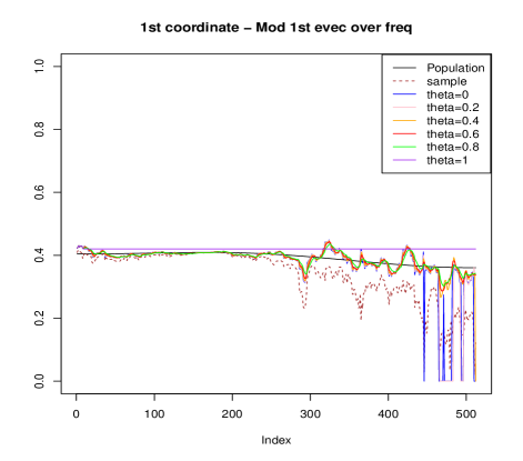
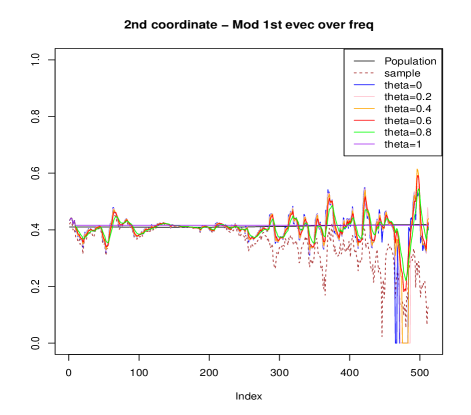
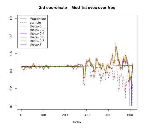
Figure 2: Leading eigenvector trajectories for the unfiltered version of the AR(2) process in case 1. Index $k$ corresponds to frequency $2\pi k/n$ for $k=1:\dots,n/2$.

	$n=2048$				$n=4096$
	$p=64$		$p=128$		$p=64$		$p=128$
	mean	sd	mean	sd	mean	sd	mean	sd
$\theta=0$	28.98	4.28	34.35	4.00	44.13	5.74	48.55	4.73
$\theta=0.2$	25.28	6.43	32.43	7.37	39.83	9.63	48.69	9.67
$\theta=0.4$	21.87	8.19	29.58	9.99	33.09	8.71	42.27	11.54
$\theta=0.6$	18.64	7.44	27.04	11.13	28.82	8.73	40.66	14.67
$\theta=0.8$	16.80	5.31	28.44	11.43	26.51	11.12	41.97	15.75
$\theta=1$	25.36	12.32	34.85	10.87	37.93	16.87	54.25	13.72

Table 3: AR(2): Frobinus norm of $\mathbf{E}_{p\times(n/2)}=[\hat{U}_{j}^{(\theta)}(\omega_{\ell})-U_{j}(\omega_{\ell})]_{j=1,\ell=1}^{p,n/2}$

	$n=2048$				$n=4096$
	$p=64$		$p=128$		$p=64$		$p=128$
	mean	sd	mean	sd	mean	sd	mean	sd
$\theta=0$	29.66	4.64	33.24	3.88	41.97	5.79	47.75	4.93
$\theta=0.2$	26.61	8.13	31.94	7.48	37.42	8.57	44.69	9.67
$\theta=0.4$	22.53	8.67	29.71	9.69	31.35	11.09	43.96	14.40
$\theta=0.6$	20.55	10.23	29.05	12.48	27.25	12.01	42.56	17.54
$\theta=0.8$	20.35	11.78	28.37	11.89	24.10	11.91	38.48	18.10
$\theta=1$	26.01	11.91	35.51	10.36	34.8	18.07	52.28	15.09

Table 4: AR(4): Frobinus norm of $\mathbf{E}_{p\times(n/2)}=[\hat{U}_{j}^{(\theta)}(\omega_{\ell})-U_{j}(\omega_{\ell})]_{j=1,\ell=1}^{p,n/2}$

6 Data Analysis

Evidence suggests that electrophysiological activity at different frequencies and locations of the brain can be biomarkers for schizophrenia and for first-episode psychosis (FEP) (Renaldi et al., 2019; Zhang et al., 2021). To illustrate the use of LSPCA to obtain interpretable frequency-channel analyses, we apply it separately to two resting state 64-channel electroencephalography (EEG) recordings: one from a patient who is experiencing FEP and has been emitted to the emergency department of the Western Psychiatric Hospital of the University of Pittsburgh Medical Center, and one from a healthy control (HC). During the recording, participants sat in a chair and relaxed with their eyes open. Data were recorded using 10-10 system and were initially sampled at a rate of 250 Hz for one minute. Pre-processing consisted of down-sampling to 64 Hz and filtering using a 1 Hz high-pass filter and 58 Hz low-pass filter; removal of segments with large artifacts such as muscle activity or movements by a trained EEG data manager; and further removal of subtle artifacts such as ocular movement and cardiac signals via independent component analysis (Delorme and Makeig, 2004).

We applied the LSPCA algorithm with sparsity and smoothing parameters selected using 2-folds cross validation, and the frequency parameter was selected using AIC. A sparsity level of $\hat{s}=8$ was selected for both subjects, smoothing parameters of $\theta=0.2$ and $\theta=0.6$ were selected and localization parameters of $\eta=41$ and $\eta=52$ were selected for the FEP and HC participants, respectively. Inspection of the scree plots at all frequencies suggests that $d=2$.

We explored the results of the analysis in two manners. First, we investigated the loadings for the real and imaginary parts of the $d=2$ components as functions of coordinate/channel and frequency for the FEP participant in Figure 3 and for the healthy control in Figure 4. Principal subspaces for both participants are localized within the union of a band of low frequencies in the $\delta$-band less than 1 Hz and band within $\theta$-frequencies between 3.5 - 5.5 Hz. As power within the $\delta$-band is characteristic of unconscious processes and elevated during rest, and power within the $\theta$-band is involved in cognitive processes such as attention control that is elevated when eyes are open, this localization is not unexpected. However, as opposed to collapsing power within the historically defined $\delta$ and $\theta$ bands of 0.5 - 4 Hz and 4 - 7 Hz, the data-driven LSPCA identified narrower, more parsimonious bands.

Next, we explore the spatial localization of power within these identified bands. Figures 5 and 6 display the diagonal elements of $\sum_{\omega\in B}\hat{\mathbf{f}}_{\vartheta}(\omega)$ where B is the localized frequency band. The results indicate different activity patterns in the FEP and HC subjects. For instance, for the HC, central channels are more active over both $\delta$ and $\theta$ frequency band. In contrast, the frontopolar and parietal channels are more active over $\delta$ band in FEP subject and central channels show more activity over the $\theta$ band. The observed difference in brain activity between the FEP and HC participants have also been reported by other investigators. For instance, in a longitudinal case-control study of FEP subjects, Renaldi et al. (2019), investigators found that the resting state EEG of FEP subjects show significantly higher power over Delta band in the frontal and posterior regions compared to the control group.

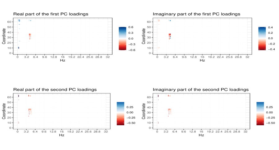
Figure 3: Subject FEP: Top left panel Real part of the first PC loadings; Top right pane: Imaginary part of the first PC loadings. Bottom left panel Real part of the second PC loadings; Bottom right pane: Imaginary part of the second PC loadings.

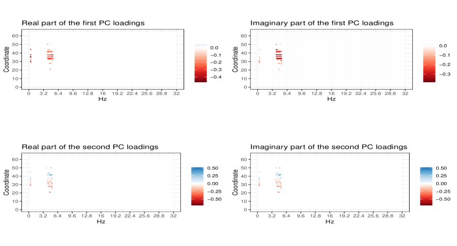
Figure 4: Subject HC: Top left panel Real part of the first PC loadings; Top right pane: Imaginary part of the first PC loadings. Bottom left panel Real part of the second PC loadings; Bottom right pane: Imaginary part of the second PC loadings.

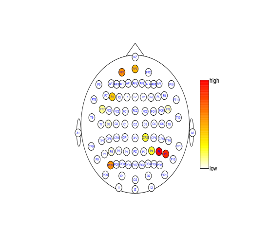
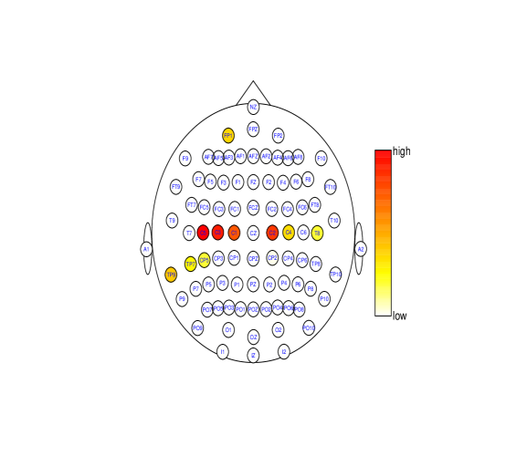
Figure 5: Active channels in FEP subject: Left panel: Delta wave frequency components; Right panel: Theta wave frequency components.

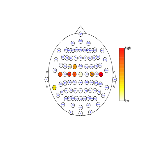
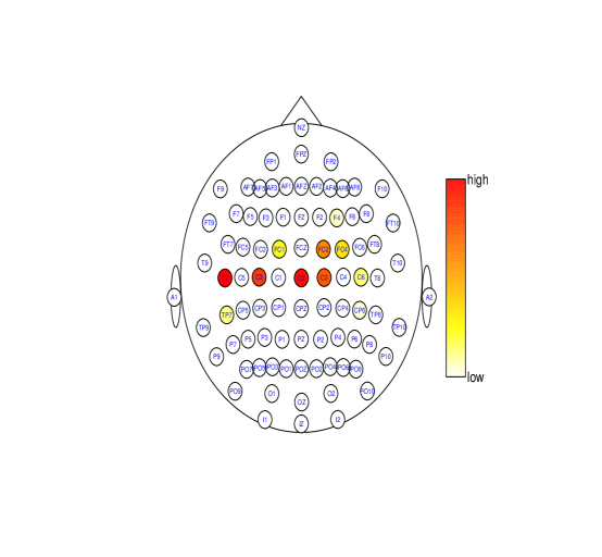
Figure 6: Active channels in HC subject: Left panel: Delta wave frequency components; Right panel: Theta wave frequency components.

7 Discussion

This article introduced what is, to the best of our knowledge, the first approach to conducting a PCA on a high-dimensional stationary time series whose principal subspace is sparse among variates, localized within frequency, and smooth as a function of frequency. The method is by no means exhaustive and can potentially be extended to more complex scenarios. The first of these is to nonstationary time series. Although the developed LSPCA routine could be applied directly using quadratic time-frequency transformations such as the local Fourier periodogram or SLeX periodogram, it is not yet obvious how to impose sparsity, frequency localization, or smoothness on the time-frequency subspaces that accounts for temporal ordering and information. A second extension is to the replicated time series setting in which a joint analysis is conducted on data where multivariate time series are observed for multiple subjects. As opposed to the analysis presented in Section 6, where separate PCAs were conducted individually for two separate subjects, a PCA for replicated time series will find optimal eigenspaces for describing mutual and subject specific information. Lastly, the proposed LSPCA offers a regularized estimation approach. One might desire a confidence-based procedure that provides inference with regards to included frequency bands and retained channels. Although the excursion set method that has been used to obtain inference for spatial clusters in image data appears to provide a natural solution for conducting inference with regards to frequency localization (Maullin-Sapey et al., 2023), how to do this while imposing sparsity and extract the low-dimensional principal subspace could prove to be challenging.

SUPPLEMENTARY MATERIAL

Algorithms:

The ADMM for solving (7), the SOAP, and the LSPCA Algorithms are outlined. In addition, the sparsity, localization, and smoothing parameter selection procedures are outlined.

Proofs:

Details of the theoretical analysis and proofs of the theorems in the paper are provided.

Appendix A Algorithms

In section A.1 the ADMM, SOAP, and the LSPCA algorithms are illustrated. Detailed description of the localization, sparsity, and smoothing parameter selection are provided in Sections A.2, A.3, and A.4, respectively.

A.1 LSPCA

Input: Spectral density estimator $\hat{\mathbf{\Sigma}}$

Output: $\mathbf{U}^{init}$

Parameters : Regularization parameter $\rho>0$, penalty parameter $\beta>0$, maximum number of iterations $T$

Initialization : $\mathbf{\Pi}^{(0)}\leftarrow 0$, $\mathbf{\Phi}^{(0)}\leftarrow 0$, $\mathbf{\Theta}^{(0)}\leftarrow 0$

for $t=0,\dots,T-1$ do

       $\mathbf{\Pi}^{t+1}\leftarrow\mbox{argmin }\{\mathcal{L}(\mathbf{\Pi},\mathbf{\Phi}^{(t)},\mathbf{\Theta}^{(t)}+\beta/2\|\mathbf{\Pi}-\mathbf{\Phi}^{(t)}\|_{F}^{2}\;|\;\mathbf{\Pi}\in\mathcal{A}\}$

       $\mathbf{\Phi}^{t+1}\leftarrow\mbox{argmin }\{\mathcal{L}(\mathbf{\Pi}^{(t+1)},\mathbf{\Phi},\Theta^{(t)})+\beta/2\|\mathbf{\Pi}^{(t+1)}-\mathbf{\Phi}\|_{F}^{2}\;|\;\mathbf{\Phi}\in\mathbb{R}^{p\times p}\}$

       $\mathbf{\Theta}^{(t+1)}\leftarrow\mathbf{\Theta}^{(t)}-\beta(\mathbf{\Pi}^{(t+1)}-\mathbf{\Phi}^{(t+1)})$

      

end for

$\bar{\mathbf{\Pi}}^{(T)}=\frac{1}{T}\sum_{t=0}^{T}\mathbf{\Pi}^{(t)}$

Set the columns of $U^{init}$ to be the top $q$ leading eigenvectors of $\bar{\mathbf{\Pi}}^{(T)}$

Output: $\mathbf{U}^{init}$

Algorithm 1 ADMM : Solving (7)

Input: $\mathbf{\Phi}^{(t)},\mathbf{\Theta}^{(t)},\hat{\mathbf{\Sigma}},\beta$

Output: $\mathbf{\Pi}^{(t+1)}$

Function Projection($\mathbf{\Phi}^{(t)},\mathbf{\Theta}^{(t)},\hat{\mathbf{\Sigma}},\beta$)

       Eigenvalue Decomposition: $\mathbf{A}\mathbf{\Lambda}\mathbf{Q}^{*}\leftarrow\mathbf{\Phi}^{(t)}+\mathbf{\Theta}^{(t)}/\beta+\hat{\mathbf{\Sigma}}/\beta$

       $(v_{1}^{\prime},\dots,v_{p}^{\prime})=\mbox{argmin}\{\|v-diag(\mathbf{\Lambda}^{(t)})\|_{2}^{2}\;|\;v\in\mathbb{R}^{p},\sum_{j}v_{j}=q,v_{j}\in[0,1]\mbox{ for all }j\}$

       $\mathbf{\Pi}^{(t+1)}\leftarrow\mathbf{Q}\mbox{diag}\{v_{1}^{\prime},\dots,v_{p}^{\prime}\}\mathbf{Q}^{*}$

       return $\mathbf{\Pi}^{(t+1)}$

return

Algorithm 2 Projection

Input: $\mathbf{\Pi}^{(t+1)},\mathbf{\Theta}^{(t)},\rho,\beta$

Output: $\mathbf{\Phi}^{(t+1)}$

for $i,j\in\{1,\dots,d\}$ do

       $\mathbf{\Phi}^{(t+1)}\leftarrow\begin{cases}0&\mbox{if }|\mathbf{\Pi}_{i,j}^{(t+1)}-\mathbf{\Theta}_{i,j}^{(t)}/\beta|\leq\rho/\beta\\ \mbox{sign}\left(\mathbf{\Pi}_{i,j}^{(t+1)}-\mathbf{\Theta}_{i,j}^{(t)}/\beta\right)\left(|\mathbf{\Pi}_{i,j}^{(t+1)}-\mathbf{\Theta}_{i,j}^{(t)}/\beta|-\rho/\beta\right)&\mbox{if }|\mathbf{\Pi}_{i,j}^{(t+1)}-\mathbf{\Theta}_{i,j}^{(t)}/\beta|>\rho/\beta\end{cases}$

end for

Output: $\mathbf{\Phi}^{(t+1)}$

Algorithm 3 Soft-Thresholding

In the Tightened step, the orthogonal iteration method is followed by a truncation step to enforce row-sparsity and further followed by taking another re-normalization step to enforce orthogonality.

Input: Spectral density matrix estimator $\mathbf{f}_{\Psi}(\omega)$, initialization $U^{init}$

Parameters : Sparsity parameter $\hat{s}$, Maximum number of iteration $\tilde{T}$

Initialization : $\tilde{\mathbf{U}}^{(T+1)}\leftarrow\mbox{Truncate}(\mathbf{U}^{init},\hat{s})$, $\mathbf{U}^{(T+1)}$, $\mathsf{\mathbf{R}}_{2}^{(T+1)}\leftarrow\mbox{Thin-QR}(\tilde{\mathbf{U}}^{(T+1)})$

for $t=T+1\dots,T+\tilde{T}-1$ do

       $\quad\tilde{\mathbf{V}}^{(t+1)}\leftarrow{\mathbf{f}}_{\Psi}(\omega)\mathbf{U}^{(t)}$

       $\quad\mathbf{V}^{(t+1)},\mathsf{\mathbf{R}}_{1}^{(t+1)}\leftarrow\mbox{Thin-QR}(\tilde{\mathbf{V}}^{(t+1)})$

       $\quad\tilde{\mathbf{U}}^{(t+1)}\leftarrow\mbox{Truncate}(\mathbf{V}^{(t+1)},\hat{s})$

       $\quad\mathbf{U}^{(t+1)},\mathsf{\mathbf{R}}_{2}^{(t+1)}\leftarrow\mbox{Thin-QR}(\tilde{\mathbf{U}})^{(t+1)}$

      

end for

Output: $\mathbf{U}^{T+\tilde{T}}$

Algorithm 4 SOAP

Function Truncate($\mathbf{V}^{(t+1)},\hat{s}$)

       Row Sorting: $\mathcal{I}_{\hat{s}}\leftarrow\mbox{The set of row index $i$`s corresponding to the top $\hat{s}$ largest $\|V_{i,.}^{(t+1)}\|_{2}$`s }$

       for $i\in\{1,\dots,p\}$ do

             $\quad\tilde{U}_{i,.}^{(t+1)}\leftarrow\mathbbm{1}[i\in\mathcal{I}_{\hat{s}}]V_{i,.}^{(t+1)}$

            

       end for

      return $\tilde{\mathbf{U}}^{(t+1)}$

return

The Truncate function, where $V_{i,.}$ denotes the $i$-th row vector of $\mathbf{V}$.

Algorithm 5 $\tilde{\mathbf{U}}^{(t+1)}\leftarrow\mbox{Truncate}(\mathbf{V}^{(t+1)},\hat{s})$ :

The Truncate function, where $V_{i,.}$ denotes the $i$-th row vector of $\mathbf{V}$.

The combined algorithm is as follows

Input: $\{\mathbf{f}_{\Psi}(\omega_{\ell})\}_{\ell=1}^{n/2}$

Parameters : Regularization parameter $\rho>0$, penalty parameter $\beta>0$, maximum number of iterations of ADMM $T$, Sparsity parameter $\hat{s}$, Maximum number of iteration of SOAP $\tilde{T}$

ADMM: $\mathbf{\Pi}_{1}\leftarrow\mbox{ADMM}(\mathbf{f}_{\Psi}(\omega_{1}))$

Set the columns of $\mathbf{U}^{init}$ to be the top $d$ leading eigenvectors of $\mathbf{\Pi}_{1}$

$\tilde{\mathbf{U}}^{(0)}\leftarrow\mbox{Truncate}(\mathbf{U}^{init},\hat{s})$, $\mathbf{U}^{init}\leftarrow\mbox{Thin-QR}(\tilde{\mathbf{U}}^{(0)})$

$\hat{\mathbf{U}}^{(0)}\leftarrow\mbox{SOAP}(\mathbf{f}_{\Psi}(\omega_{1}),\mathbf{U}^{init})$

for $\ell\in\{1,\dots,n/2-1\}$ do

       $\quad\hat{\mathbf{U}}(\omega_{\ell+1})\leftarrow\mbox{SOAP}(\mathbf{f}_{\Psi}(\omega_{\ell+1}),\hat{\mathbf{U}}(\omega_{\ell}))$

      

end for

Output: $\{\hat{\mathbf{U}}(\omega_{\ell})\}_{\ell=1}^{n/2}$

Algorithm 6 LSPCA

A.2 Localization Parameter Selection

For selecting the localization parameter $\eta$, we propose to use information criteria based on the Whittle likelihood, or the large sample complex Gaussian distribution of the periodogram $d_{X}(\omega_{\ell})\overset{D}{\rightarrow}N^{c}\left[0,\mathbf{f}(\omega_{\ell})\right]$. This is done given $d$ and initially without smoothing $\theta=0$. It can be done iteratively after updating other parameters, simulations suggest that it is robust to the selection of $s$ and $\theta$. We apply the LSPCA algorithm to obtain the eignevectors $\hat{U}_{j}(\omega)$, $j=1,\dots,d$, which are used to compute the estimator of the spectrum of the $d$-dimensional principle series

$$\hat{\mathbf{f}}_{\vartheta}(\omega_{\ell})=\mathbf{f}_{\Psi}(\omega_{\ell})\hat{U}_{1}(\omega_{\ell})\hat{U}_{1}(\omega_{\ell})^{\dagger}+\dots+\mathbf{f}_{\Psi}(\omega_{\ell})\hat{U}_{d}(\omega_{\ell})\hat{U}_{d}(\omega_{\ell})^{\dagger},$$

Let $\check{L}_{\kappa}=\{\ell_{(1)},\dots,\ell_{(\kappa)}\}\in\check{L}:=\{1,2,\dots,n/2\}$ be the index set of all fundamental frequencies that are selected to be above a threshold given a localization parameter $\eta$. Our desire to to select $\eta$ such that the power from the principle series that are not distinguishable from average power from the residual series are not maintained. We estimate average power in the residual series $\epsilon(t)$ as $\hat{\mathbf{\Sigma}}=\sum_{\ell\in\check{L}/\check{L}_{\kappa}}d_{X}(\omega_{\ell})d_{X}(\omega_{\ell})^{\dagger}/\left(|\check{L}|-|\check{L}_{\kappa}|\right)$, and consider the estimated spectral density matrices where $\hat{\mathbf{G}}_{\ell}=\hat{\mathbf{f}}^{(d)}_{\vartheta}(\omega_{\ell})+\hat{\mathbf{\Sigma}}$ for $\ell\in\check{L}_{\kappa}$, and $\hat{\mathbf{\Sigma}}_{\ell}$ for $\ell\notin\check{L}_{\kappa}$. The log-Whittle likelihood estimated by

$$\log(\mathcal{L})=-\sum_{\ell=1}^{n/2}\{p\log{\pi}+\log{|\hat{\mathbf{G}}_{\ell}|}+[d_{X}(\omega_{\ell})][\hat{\mathbf{G}}_{\ell}]^{-1}[d_{X}(\omega_{\ell})]^{\dagger}\},$$

which we use to define standard information criteria for $\eta$ including $AIC=-2\log(\mathcal{L})+2|L_{K}|$, $AICc=-2\log(\mathcal{L})+2|L_{K}|+\frac{2|L_{K}|^{2}+2|L_{K}|}{n-|L_{K}|-1}$, and $BIC=-2\log(\mathcal{L})+\log(n)|L_{K}|$. The localization parameter $\eta$ is selected to minimizing an information criteria.

A.3 Sparsity Parameter Selection

For selecting the sparsity level of the underlying process, we propose to use $k$-folds cross validation, with the Mahalanobis distance to evaluate the performance of fitted model in the validation step. The procedure splits the data into $k$ blocks, or folds, of length $n/k$, and define the time series form the $r$th fold as $X^{(r)}(t)=X\left[t-\left(r-1\right)n/k\right]$, $t=(r-1)n/k+1$, $r=1,\dots,k$. To make sure fundamental frequencies in the training and validation step match, $n$ should be divisible by $k$. In addition, let $\mathbf{f}_{\Psi}^{(1)}(\omega),\dots,\mathbf{f}_{\Psi}^{(k)}(\omega)$ be the estimated spectral density matrices obtained from each partition. We consider

$$\mathbf{f}_{\Psi}^{(-r)}(\omega)=\frac{1}{r-1}\sum_{j\neq r}\mathbf{f}_{\Psi}^{(j)}(\omega)$$ (18)

as an estimate of the spectral density matrix $\mathbf{f}(\omega)$ removing data from the $r$th fold. We then define the rank-d principal subspace spectrum estimate $\hat{\mathbf{f}}^{(r)}$, average power from the residual series $\hat{\mathbf{\Sigma}}^{(r)}$, and spectral matrix estimate $\hat{\mathbf{G}}^{(r)}_{\ell}$ for data outside of the $r$th fold in a manner analogous to the definitions in Section A.2 using all data.

We then consider the Mahalbanois distance between the discrete Fourier transform of the data from the $r$th fold from the estimated spectral matrix from the rest of the data at the $\ell$th frequency

$$\mathcal{D}\left[d_{X^{(r)}}(\omega_{\ell})\right]=d_{X^{(r)}}(\omega_{\ell})[\hat{\mathbf{G}}_{\ell}^{(r)}]^{-1}d_{X^{(r)}}(\omega_{\ell})^{\dagger},$$

and average over folds and frequencies to estimate he average Mahalbanois distance

$$\bar{\mathcal{D}}(s)=\frac{1}{k}\sum_{1=1}^{k}\sum_{\ell=1}^{n/(2k)}\mathcal{D}\left[d_{X^{(r)}}(\omega_{\ell})\right].$$ (19)

We select the sparsity level $\hat{s}$ that minimizes this distance

$$\hat{s}=\operatorname*{arg\,min}_{s}\bar{\mathcal{D}}(s).$$ (20)

A.4 Smoothing Parameter Selection

We select the smoothing parameter $\theta$ using $k$-folds cross validation, with the Mahalanobis distance to evaluate the performance of fitted model in the validation step. The procedure is similar to the procedure for the selection of the sparsity, but considers a fixed value of sparsity and varying levels of $\theta$.

Appendix B Proofs

Appendix B is devoted to the proof of the Theorems presented in this paper. We first present the model and the assumptions under which we developed the theory in Section B.1. This is followed by the proof of the main theoretical results provided in section B.2. Section B.2.1 contains a proof for Proposition (3.1)). In Section B.2.2 we present a proof for Theorem (3) part (I). Proof of part (II) of Theorem (3) is presented in Section B.2.3. Proofs of the main results follow from the Theorems and Lemmas that are presented in Section B.3 (Preliminary Theorems and Lemmas). Appendix B is concluded with some background Definitions and Lemmas.

B.1 Model Assumptions

let $\mathcal{M}_{d}(f,d,s^{*})$ be the class of $p$-dimensional stationary time series $\{X(t):t\in\mathbb{Z}\}$ satisfying the following assumptions.

Assumption 1.

For all $\omega\in[0,1)$, the $d$-dimensional principal subspace of $\mathbf{f}(\omega)$ is $s^{*}$-sparse.

Assumption 2.

There exists constants $c_{1}$ and $\gamma_{1}\geq 1$ such that for all $h\geq 1$, the $\alpha$-mixing coefficient satisfies

$$\alpha(h)\leq\exp\{-c_{1}h^{\gamma_{1}}\}$$ (21)

Assumption 3.

There exists positive constants $c_{2}$ and $\gamma_{2}$ such that for all $v\in\mathbb{S}^{p-1}(\mathbb{C})$ and all $\lambda\geq 0$, we have

$$\mathbb{P}\left(|v^{*}X(t)|\geq\lambda\right)\leq 2\exp\{-c_{2}\lambda^{\gamma_{2}}\},\quad\mbox{ for all }t\in\mathbb{Z},$$ (22)

where $\mathbb{S}^{p-1}(\mathbb{C})$ is the unit ball of dimension $p$.

Assumption 4.

Define $\gamma$ via $\frac{1}{\gamma}=\frac{1}{\gamma_{1}}+\frac{2}{\gamma_{2}}$, where $\gamma_{1}$ and $\gamma_{2}$ are given in assumptions (2) and (3). We assume that $\gamma<1$.

B.2 Proof of the Main Results

B.2.1 Proof of Proposition (3.1)

Proof.

We prove the claim by induction. First note that the objective function is increasing in $\beta_{j}$‘s and thus the maximum is attained at $\sum_{\ell=1}^{K}\beta_{\ell}=\eta$.
When $K=2$, and $\eta=1$, order $h_{1},h_{2}$ in decreasing order as $h_{(1)},h_{(2)}$ and their corresponding coefficients as $\beta_{(1)}$ and $\beta_{(2)}$. Note that $\beta_{1}+\beta_{2}=1$ and

$$h_{(1)}=\beta_{(1)}h_{(1)}+(1-\beta_{(1)})h_{(1)}>\beta_{(1)}h_{(1)}+(1-\beta_{(1)})h_{(2)}=\beta_{(1)}h_{(1)}+\beta_{(2)}h_{(2)}.$$

For any $\eta<K$ assume that the claim of the proposition hols for any $h_{1},\dots,h_{K}\in\mathbb{R}^{+}$. Since $\sum_{\ell=1}^{K}\beta_{\ell}=\eta$ and $0\leq\beta_{\ell}\leq 1,\ell=1,\dots,K$, by the induction hypothesis we have

$$\sum_{j=1}^{\eta}h_{(j)} >\sum_{j=1}^{K-1}\beta_{(j)}h_{(j)}+(\beta_{(K)}+\beta_{(K+1)})h_{(K)}$$

$$>\sum_{j=1}^{K+1}\beta_{(j)}h_{(j)}.$$

The second inequality holds since $h_{(K)}\geq h_{K+1}$. This shows that for $K+1$ the optimum is attained at $\beta_{(1)}=\dots=\beta_{(\eta)}=1,\beta_{(\eta+1)}=\dots=\beta_{(K)}=\beta_{(K+1)}=0$ hence, by induction, the claim follows for any $K\in\mathbb{N}$. This shows that when $\eta$ is fixed, for any $K$ the conclusion of the theorem holds.

Now, we show that the result holds for any $\eta$. For $K=2$ the result is trivial. For any $K\geq 3$ set $\eta=1$, then

$$(1-\beta_{(1)})h_{(1)}=(\beta_{(2)}+\beta_{(3)}+\dots+\beta_{(K)})h_{(1)}\geq\beta_{(2)}h_{(2)}+\beta_{(3)}h_{(3)}+\dots+\beta_{(K)}h_{(K)}$$ (23)

showing that $h_{(1)}\geq\beta_{(1)}h_{(1)}+\beta_{(2)}h_{(2)}+\dots+\beta_{(K)}h_{(K)}$, for any $0\geq\beta_{1},\dots,\beta_{K}\geq 1$ such that $\beta_{1}+\dots+\beta_{K}=1$. Suppose the conclusion of the theorem holds for an $\eta\leq K$ we show that the conclusion also holds for $\eta+1$.

For $\eta+1$ By the assumptions of the theorem, $\beta_{(1)}+\dots+\beta_{(K)}=\eta+1$, therefore, $\eta+1\geq\beta_{(2)}+\dots+\beta_{(K)}\geq\eta$. Let $1\geq\alpha:=\beta_{(2)}+\dots+\beta_{(K)}-\eta\geq 0$. Note that $\beta_{(1)}+\alpha=1$. Since the for $K=2,\eta=1$ the conclusion of the theorem holds, we have

$$h_{(1)}\geq\beta_{(1)}h_{(1)}+\alpha(h_{(2)}+\dots+h_{(K)})$$ (24)

In addition, for any $\tilde{\beta}_{(2)},\dots,\tilde{\beta}_{(K)}$ such that $\tilde{\beta}_{(2)}+\dots+\tilde{\beta}_{(K)}=\eta$, by the indication hypothesis, we have

$$h_{(2)}+\dots+h_{(\eta+1)}\geq\tilde{\beta}_{(2)}h_{(2)},\dots,\tilde{\beta}_{(K)}h_{(K)}.$$ (25)

In particular, for any choice of $0\leq\tilde{\beta}_{(2)},\dots,\tilde{\beta}_{(K)}\leq 1$ such that $\tilde{\beta}_{(2)}+\dots+\tilde{\beta}_{(K)}=\eta$ and

$$\tilde{\beta}_{(2)}+\dots+\tilde{\beta}_{(K)}+\alpha=\beta_{(2)}+\beta_{(3)}+\dots+\beta_{(K)}$$

we conclude that

$$h_{(1)}+h_{(2)}+\dots+h_{(\eta+1)} \geq\beta_{(1)}h_{(1)}+(\tilde{\beta}_{(2)}+\alpha)h_{(2)},\dots,(\tilde{\beta}_{(K)}+\alpha)h_{(K)}$$ (26)

$$\geq\beta_{(1)}h_{(1)}+\beta_{(2)}h_{(2)}+\dots+\beta_{(K)}h_{(K)}.$$ (27)

Hence, by indication, the result follows for any $K$ and for any $\eta\leq K$. ∎

B.2.2 Proof of Theorem (3) part (I)

Proof.

Let $\mathbf{U}_{\ell}^{(t)}$ and $\mathbf{U}_{\ell}^{*}$ be orthonormal matrices whose columns span $\mathcal{U}^{(t)}(\omega_{1})$ and $\mathcal{U}^{*}(\omega_{1})$, respectively. In addition, let $\mathbf{\Pi}_{\ell}^{(t)}=\mathbf{U}_{\ell}^{(t)}[\mathbf{U}_{\ell}^{(t)}]^{\dagger}$ and $\mathbf{\Pi}_{\ell}^{*}=\mathbf{U}_{\ell}^{*}[\mathbf{U}_{\ell}^{*}]^{\dagger}$ be the corresponding projection matrices. Note that

$$\mathcal{D}(\mathcal{U}^{(t)}(\omega_{1}),\mathcal{U}^{*}(\omega_{1})) =\|\Pi_{\ell}^{(t)}-\Pi_{\ell}^{*}\|_{F}$$

$$=\|(\Re{(\mathbf{U}_{\ell}^{(t)})}+i\Im{(\mathbf{U}_{\ell}^{(t)})})(\Re{([\mathbf{U}_{\ell}^{(t)}]^{\dagger})}-i\Im{([\mathbf{U}_{\ell}^{(t)}]^{\dagger})})$$

$$\quad-(\Re{(\mathbf{U}_{\ell}^{*})}+i\Im{(\mathbf{U}_{\ell}^{*})})(\Re{([\mathbf{U}_{\ell}^{*}]^{\dagger})}-i\Im{([\mathbf{U}_{\ell}^{*}]^{\dagger})}\|_{F}$$

$$=\|\Re{(\mathbf{U}_{\ell}^{(t)})}\Re{([\mathbf{U}_{\ell}^{(t)}]^{\dagger})}-\Re{(\mathbf{U}_{\ell}^{*})}\Re{([\mathbf{U}_{\ell}^{*}]^{\dagger})}+\Im{(\mathbf{U}_{\ell}^{(t)})}\Im{([\mathbf{U}_{\ell}^{(t)}]^{\dagger})}-\Im{(\mathbf{U}_{\ell}^{*})}\Im{([\mathbf{U}_{\ell}^{*}]^{\dagger})}$$

$$+i\{-\Re{(\mathbf{U}_{\ell}^{(t)})}\Im{([\mathbf{U}_{\ell}^{(t)}]^{\dagger})}+\Re{(\mathbf{U}_{\ell}^{*})}\Im{([\mathbf{U}_{\ell}^{*}]^{\dagger})}+\Im{(\mathbf{U}_{\ell}^{(t)})}\Re{([\mathbf{U}_{\ell}^{(t)}]^{\dagger})}-\Im{(\mathbf{U}_{\ell}^{*})}\Re{([\mathbf{U}_{\ell}^{*}]^{\dagger})}\}\|_{F}$$

$$\leq\|\Re{(\mathbf{U}_{\ell}^{(t)})}\Re{([\mathbf{U}_{\ell}^{(t)}]^{\dagger})}-\Re{(\mathbf{U}_{\ell}^{*})}\Re{([\mathbf{U}_{\ell}^{*}]^{\dagger})}\|_{F}+\|\Im{(\mathbf{U}_{\ell}^{(t)})}\Im{([\mathbf{U}_{\ell}^{(t)}]^{\dagger})}-\Im{(\mathbf{U}_{\ell}^{*})}\Im{([\mathbf{U}_{\ell}^{*}]^{\dagger})}\|_{F}$$

$$+\|\Re{(\mathbf{U}_{\ell}^{(t)})}\Im{([\mathbf{U}_{\ell}^{(t)}]^{\dagger})}-\Re{(\mathbf{U}_{\ell}^{*})}\Im{([\mathbf{U}_{\ell}^{*}]^{\dagger})}\|_{F}+\|\Im{(\mathbf{U}_{\ell}^{(t)})}\Re{([\mathbf{U}_{\ell}^{(t)}]^{\dagger})}-\Im{(\mathbf{U}_{\ell}^{*})}\Re{([\mathbf{U}_{\ell}^{*}]^{\dagger})}\|_{F}$$

$$\overset{(i)}{\leq}2\left\|\begin{bmatrix}\Re{(\mathbf{U}_{\ell}^{(t)})}\\ \Im{(\mathbf{U}_{\ell}^{(t)})}\end{bmatrix}\begin{bmatrix}\Re{([\mathbf{U}_{\ell}^{(t)}]^{\dagger})}&\Im{([\mathbf{U}_{\ell}^{(t)}]^{\dagger})}\end{bmatrix}-\begin{bmatrix}\Re{(\mathbf{U}_{\ell}^{*})}\\ \Im{(\mathbf{U}_{\ell}^{*})}\end{bmatrix}\begin{bmatrix}\Re{([\mathbf{U}_{\ell}^{*}]^{\dagger})}&\Im{([\mathbf{U}_{\ell}^{*}]^{\dagger})}\end{bmatrix}\right\|_{F}$$

$$=2\mathcal{D}([\mathcal{U}^{(t)}(\omega_{1})]^{(R)},[\mathcal{U}^{*}(\omega_{1})]^{(R)})$$

Note that $(i)$ holds since

$$\left\|\begin{bmatrix}\mathbf{A}&\mathbf{B}\\ \mathbf{B}^{\dagger}&\mathbf{D}\end{bmatrix}\right\|_{F}=\sqrt{\|\mathbf{A}\|_{F}^{2}+\|\mathbf{B}\|_{F}^{2}+\|\mathbf{B}^{\dagger}\|_{F}^{2}+\|\mathbf{D}\|_{F}^{2}}$$

and

$$\|\mathbf{A}\|_{F}+\|\mathbf{B}\|_{F}+\|\mathbf{C}\|_{F}+\|\mathbf{D}\|_{F}\leq 2\sqrt{\|\mathbf{A}\|_{F}^{2}+\|\mathbf{B}\|_{F}^{2}+\|\mathbf{B}^{\dagger}\|_{F}^{2}+\|\mathbf{D}\|_{F}^{2}}.$$

Thus the result follows from Theorem (7) with $\tilde{\tilde{C}}^{\prime}=2\tilde{C}^{\prime}$ and $\tilde{\tilde{C}}^{\prime\prime}=2\tilde{C}^{\prime\prime}$.

∎

B.2.3 Proof of Theorem (3) part (II)

Remark 4 (Notation).

We denote the estimator of the spectral density matrix considered in the theorem as $\hat{\mathbf{f}}_{M}^{(\theta)}$ which belongs to the general class of estimators $\mathbf{f}_{\Psi}$.

$$\hat{\mathbf{f}}_{M}^{(\theta)} =(1-\theta)\hat{\mathbf{f}}_{M}(\omega_{\ell+1})+\theta\;\hat{\mathbf{\Pi}}_{\ell}\hat{\mathbf{f}}_{M}(\omega_{\ell+1})\hat{\mathbf{\Pi}}_{\ell}$$

$$\hat{\mathbf{f}}_{M} =\sum_{t=-M}^{M}\hat{\mathbf{R}}_{t}\exp\{-2\pi i\omega t\}$$

$$\hat{\mathbf{R}}_{t} =\frac{1}{n}\sum_{k=1}^{n-t}X(k+t)X(t)^{\dagger}$$

where $\hat{\mathbf{\Pi}}_{\ell}$ is the estimated $d$-dimensional principal subspace of $\mathbf{f}(\omega_{\ell})$ obtained from the LSPCA algorithm.

Let $\mathcal{U}^{*}_{\ell}$ be the $d$-dimensional principal subspace of $\mathbf{f}(\omega_{\ell})$ and $\mathbf{U}^{*}_{\ell}$ be an orthonormal matrix such that its columns span $\mathcal{U}^{*}_{\ell}$. In addition, let $\mathcal{S}^{*}$ be the row-support of $\mathbf{U}^{*}_{\ell}$ and $\mathcal{I}\subseteq\{1,\dots,p\}$ be an index set. Let $\hat{\mathbf{f}}_{M}^{(\theta)}(\omega_{\ell},\mathcal{I})$ be the restriction of $\hat{\mathbf{f}}_{M}^{(\theta)}(\omega_{\ell})$ onto the columns and rows indexed by $\mathcal{I}$ and $\hat{\mathbf{U}}_{\ell}(\mathcal{I})$ be the orthonormal matrix with columns consisting of the top $d$ leading eigenvectors of $\hat{\mathbf{f}}_{M}^{(\theta)}(\omega_{\ell},\mathcal{I})$. Also, let $\hat{\mathcal{U}}(\omega_{\ell},\mathcal{I})$ be the space spanned by the columns of $\hat{\mathbf{U}}_{\ell}(\mathcal{I})$. By the QR decomposition step in the Algorithm SOAP, $\hat{\mathbf{f}}_{M}(\omega_{\ell+1},\mathcal{I})\mathbf{U}^{(t)}(\omega_{\ell+1})=\mathbf{V}^{(t+1)}(\omega_{\ell+1})\mathsf{\mathbf{R}}_{1}^{(t+1)}(\omega_{\ell+1})$. Denote the column-space of $\mathbf{V}^{(t+1)}(\omega_{\ell+1})$ by $\mathcal{V}^{(t+1)}(\omega_{\ell+1})$. In addition, let $\|A\|_{op}=\max\{v^{\dagger}Av:\|v\|_{2}=1\}$, the $(p,q)$-norm of a matrix $A$, $\|A\|_{p,q}$ be the $\ell_{q}$ norm of the $\ell_{p}$ norms of the rows of $A$, and

$$\|\hat{\mathbf{f}}^{(\theta)}_{M}(\omega_{\ell+1})-\mathbf{f}(\omega_{\ell+1})\|_{op,|\mathcal{I}|}:=\max_{\|v\|_{2}=1,|\mbox{supp}(v)|\leq\mathcal{I}}\|v^{\dagger}([\hat{\mathbf{f}}^{(\theta)}_{M}(\omega_{\ell+1})-\mathbf{f}(\omega_{\ell+1})]_{\mathcal{I}})v\|_{2}.$$ (28)

Throughout the rest of the document, we denote the eigenvalues, in decreasing order, of a $p\times p$ Hermitian matrix $H$ by $\lambda_{1}(H),\dots,\lambda_{p}(H)$ and will use $\lambda_{k}(\omega)$ to denote $\lambda_{k}(\mathbf{f}(\omega))$, for $k=1,\dots,p$.

Lemma 1.

Under the conditions of Theorem (6), we have

$$\begin{split}\|\hat{\mathbf{f}}_{M}^{(\theta)}(\omega_{\ell+1})-\mathbf{f}(\omega_{\ell+1})\|_{op,|\mathcal{I}|}&\leq\|\hat{\mathbf{f}}_{M}(\omega_{\ell+1})-\mathbf{f}(\omega_{\ell+1})\|_{op,|\mathcal{I}|}\\ &\qquad+2\theta\lambda_{1}(\omega_{\ell+1})\left[\mathcal{D}(\mathcal{U}^{*}_{\ell},\mathcal{U}^{*}_{\ell+1})+\mathcal{D}(\mathcal{U}^{*}_{\ell},\hat{\mathcal{U}}_{\ell}(\mathcal{I}))\right]+\theta\lambda_{k+1}(\omega_{\ell+1})\end{split}$$ (29)

$$\begin{split}&\leq\left(\exp(-c_{0}M(n))\vee M(n)\sqrt{\frac{s^{*}\log(p)}{n}}\right)\\ &\qquad+2\theta\lambda_{1}(\omega_{\ell+1})\left[\mathcal{D}(\mathcal{U}^{*}_{\ell},\mathcal{U}^{*}_{\ell+1})+\mathcal{D}(\mathcal{U}^{*}_{\ell},\hat{\mathcal{U}}_{\ell}(\mathcal{I}))\right]+\theta\lambda_{k+1}(\omega_{\ell+1}),\end{split}$$ (30)

where the second inequality holds with high probability.

Proof.

Let

$$\mathbf{f}^{(\theta)}(\omega_{\ell+1})=(1-\theta)\mathbf{f}(\omega_{\ell})+\theta\mathbf{\Pi}_{\ell}\mathbf{f}(\omega_{\ell+1})\mathbf{\Pi}_{\ell}.$$ (31)

Note that

$$\hat{\mathbf{f}}_{M}^{(\theta)}(\omega_{\ell+1})-\mathbf{f}(\omega_{\ell+1})=\underbrace{\hat{\mathbf{f}}_{M}^{(\theta)}(\omega_{\ell+1})-\mathbf{f}^{(\theta)}(\omega_{\ell+1})}_{(I)}+\underbrace{\mathbf{f}^{(\theta)}(\omega_{\ell+1})-\mathbf{f}(\omega_{\ell+1})}_{(II)}.$$

Note that

$$(I)=\underbrace{(1-\theta)(\hat{\mathbf{f}}_{M}(\omega_{\ell+1})-\mathbf{f}(\omega_{\ell+1}))}_{(I.1)}+\theta\underbrace{\left[\hat{\mathbf{\Pi}}_{\ell}\hat{\mathbf{f}}_{M}(\omega_{\ell+1})\hat{\mathbf{\Pi}}_{\ell}-\mathbf{\Pi}_{\ell}\mathbf{f}(\omega_{\ell+1})\mathbf{\Pi}_{\ell}\right]}_{(I.2)}$$

$$(I.2)=\hat{\mathbf{\Pi}}_{\ell}\left[\hat{\mathbf{f}}_{M}(\omega_{\ell+1})-\mathbf{f}(\omega_{\ell+1})\right]\hat{\mathbf{\Pi}}_{\ell}+\hat{\mathbf{\Pi}}_{\ell}\mathbf{f}(\omega_{\ell+1})\left(\hat{\mathbf{\Pi}}_{\ell}-\mathbf{\Pi}_{\ell}\right)+\left(\hat{\mathbf{\Pi}}_{\ell}-\mathbf{\Pi}_{\ell}\right)\mathbf{f}(\omega_{\ell+1})\mathbf{\Pi}_{\ell}.$$

By $(I.1)$ and $(I.2)$

$$\|\hat{\mathbf{f}}_{M}^{(\theta)}(\omega_{\ell+1})-\mathbf{f}^{(\theta)}(\omega_{\ell+1})\|_{op,|\mathcal{I}|}\leq\|\hat{\mathbf{f}}_{M}(\omega_{\ell+1})-\mathbf{f}(\omega_{\ell+1})\|_{op,|\mathcal{I}|}+2\theta\lambda_{1}(\omega_{\ell+1})\mathcal{D}(\mathcal{U}^{*}_{\ell},\hat{\mathcal{U}}_{\ell}(\mathcal{I}))$$ (32)

Also,

$$(II) =\theta\left[\mathbf{\Pi}_{\ell}\mathbf{f}(\omega_{\ell+1})\mathbf{\Pi}_{\ell}-\mathbf{f}(\omega_{\ell+1})\right]$$

$$=\theta\left[\mathbf{\Pi}_{\ell}\mathbf{f}(\omega_{\ell+1})\mathbf{\Pi}_{\ell}-\mathbf{\Pi}_{\ell}\mathbf{f}(\omega_{\ell+1})\mathbf{\Pi}_{\ell+1}+\mathbf{\Pi}_{\ell}\mathbf{f}(\omega_{\ell+1})\mathbf{\Pi}_{\ell+1}-\mathbf{\Pi}_{\ell+1}\mathbf{f}(\omega_{\ell+1})\mathbf{\Pi}_{\ell+1}-\mathbf{\Pi}_{\ell+1}^{\perp}\mathbf{f}(\omega_{\ell+1})\mathbf{\Pi}_{\ell+1}^{\perp}\right]$$

$$=\theta\left[\mathbf{\Pi}_{\ell}\mathbf{f}(\omega_{\ell+1})(\mathbf{\Pi}_{\ell}-\mathbf{\Pi}_{\ell+1})+(\mathbf{\Pi}_{\ell}-\mathbf{\Pi}_{\ell+1})\mathbf{f}(\omega_{\ell+1})\mathbf{\Pi}_{\ell+1}-\mathbf{\Pi}_{\ell+1}^{\perp}\mathbf{f}(\omega_{\ell+1})\mathbf{\Pi}_{\ell+1}^{\perp}\right].$$

Thus,

$$\|\mathbf{f}^{(\theta)}(\omega_{\ell+1})-\mathbf{f}(\omega_{\ell+1})\|_{op,|\mathcal{I}|}\leq 2\theta\lambda_{1}(\omega_{\ell+1})\mathcal{D}(\mathcal{U}^{*}_{\ell},\mathcal{U}^{*}_{\ell+1})+\theta\lambda_{d+1}(\omega_{\ell+1}).$$

Hence,

$$\|\hat{\mathbf{f}}_{M}^{(\theta)}(\omega_{\ell+1})-\mathbf{f}(\omega_{\ell+1})\|_{2,|\mathcal{I}|} \leq\|\hat{\mathbf{f}}_{M}(\omega_{\ell+1})-\mathbf{f}(\omega_{\ell+1})\|_{2,|\mathcal{I}|}$$ (33)

$$\qquad+2\theta\lambda_{1}(\mathbf{f}(\omega_{\ell+1}))\left[\mathcal{D}(\mathcal{U}^{*}_{\ell},\mathcal{U}^{*}_{\ell+1})+\mathcal{D}(\mathcal{U}^{*}_{\ell},\hat{\mathcal{U}}_{\ell}(\mathcal{I}))\right]+\theta\lambda_{k+1}(\omega_{\ell+1})$$ (34)

$$\leq\left(\exp(-c_{0}M(n))\vee M(n)\sqrt{\frac{s^{*}\log(p)}{n}}\right)$$ (35)

$$\qquad+2\theta\lambda_{1}(\mathbf{f}(\omega_{\ell+1}))\left[\mathcal{D}(\mathcal{U}^{*}_{\ell},\mathcal{U}^{*}_{\ell+1})+\mathcal{D}(\mathcal{U}^{*}_{\ell},\hat{\mathcal{U}}_{\ell}(\mathcal{I}))\right]+\theta\lambda_{k+1}(\omega_{\ell+1}).$$ (36)

Note the second inequality is followed by Theorem (6). ∎

Lemma 2.

Under the same conditions of Theorem (6), with high probability, we have

$$\mathcal{D}(\mathcal{U}^{*}_{\ell+1},\hat{\mathcal{U}}_{\ell+1}(\mathcal{I}))\leq\frac{\mathcal{E}_{1}}{\mathcal{E}_{2}}=:\Delta_{\ell+1}(\mathcal{I}),$$ (37)

where

$$\mathcal{E}_{1} =\sqrt{2d}\left[\left(\exp(-c_{0}M(n))\vee M(n)\sqrt{\frac{s^{*}\log(p)}{n}}\right)\right.$$

$$\qquad\qquad\left.+2\theta\lambda_{1}(f(\omega_{\ell+1}))\left[\mathcal{D}(\mathcal{U}^{*}_{\ell},\mathcal{U}^{*}_{\ell+1})+\mathcal{D}(\mathcal{U}^{*}_{\ell},\hat{\mathcal{U}}_{\ell}(\mathcal{I}))\right]+\theta\lambda_{k+1}(\omega_{\ell+1})\right]$$

$$\mathcal{E}_{2} =\frac{1}{2}\left[\lambda_{d}(\omega_{\ell+1})-(1-\theta)\lambda_{d+1}(\omega_{\ell+1})\right]-2\theta\lambda_{1}(\omega_{\ell+1})\mathcal{D}(\mathcal{U}^{*}_{\ell},\hat{\mathcal{U}}_{\ell}(\mathcal{I}))$$

Proof.

Let $[\mathbf{U}_{\ell}^{*}]^{\perp}$ be the orthogonal matrix whose columns are the eigenvectors corresponding to $\lambda_{d+1}(\mathbf{f}(\omega_{\ell})),\dots,\lambda_{p}(\mathbf{f}(\omega_{\ell}))$ and let $[\hat{\mathbf{U}}_{\ell}]^{\perp}$ be the orthogonal matrix whose columns are the eigenvectors corresponding to $\lambda_{d+1}(\hat{\mathbf{f}}^{(\theta)}_{M}(\omega_{\ell},\mathcal{I})),\dots,\lambda_{p}(\hat{\mathbf{f}}^{(\theta)}_{M}(\omega_{\ell},\mathcal{I}))$. The following holds

1. $$\mathbf{f}(\omega_{\ell+1})U_{\ell+1}^{*} =\mathbf{U}_{\ell+1}^{*}\mathbf{\Lambda}_{0}(\mathbf{f}(\omega_{\ell+1}))$$

   $$\hat{\mathbf{f}}^{(\theta)}_{M}(\omega_{\ell+1},\mathcal{I})[\hat{\mathbf{U}}_{\ell+1}]^{\perp} =[\hat{\mathbf{U}}_{\ell+1}]^{\perp}\Lambda_{1}(\hat{\mathbf{f}}^{(\theta)}_{M}(\omega_{\ell+1},\mathcal{I})),$$

   where

   $$\mathbf{\Lambda}_{0}(\mathbf{f}(\omega_{\ell+1})) =\mbox{diag}\{\lambda_{d+1}(\mathbf{f}(\omega_{\ell+1})),\dots,\lambda_{p}(\mathbf{f}(\omega_{\ell+1}))\}$$

   $$\mathbf{\Lambda}_{1}(\hat{\mathbf{f}}^{(\theta)}_{M}(\omega_{\ell+1},\mathcal{I})) =\mbox{diag}\{\lambda_{d+1}(\hat{\mathbf{f}}^{(\theta)}_{M}(\omega_{\ell+1},\mathcal{I})),\dots,\lambda_{p}(\hat{\mathbf{f}}^{(\theta)}_{M}(\omega_{\ell+1},\mathcal{I}))\}$$

2. $$[\mathbf{U}_{\ell+1}^{*}]^{\dagger}[\hat{\mathbf{f}}^{(\theta)}_{M}(\omega_{\ell+1},\mathcal{I}))-\mathbf{f}(\omega_{\ell+1})][\hat{\mathbf{U}}_{\ell+1}]^{\perp} =[\mathbf{U}_{\ell+1}^{*}]^{\dagger}[\hat{\mathbf{f}}^{(\theta)}_{M}(\omega_{\ell+1},\mathcal{I}))][\hat{U}_{\ell+1}]^{\perp}-[\mathbf{f}(\omega_{\ell+1})\mathbf{U}_{\ell+1}^{*}]^{\dagger}[\hat{\mathbf{U}}_{\ell+1}]^{\perp}$$

   $$=[\mathbf{U}_{\ell+1}^{*}]^{\dagger}[\hat{\mathbf{U}}_{\ell+1}]^{\perp}\Lambda_{1}(\hat{\mathbf{f}}^{(\theta)}_{M}(\omega_{\ell+1},\mathcal{I}))$$

   $$\qquad\qquad\qquad-\mathbf{\Lambda}_{0}(\mathbf{f}(\omega_{\ell+1}))[\mathbf{U}_{\ell+1}^{*}]^{\dagger}[\hat{\mathbf{U}}_{\ell+1}]^{\perp}.$$

3. $$\|[\mathbf{U}_{\ell+1}^{*}]^{\dagger}[\hat{\mathbf{U}}_{\ell+1}]^{\perp}\|_{op} =\|\mathbf{\Lambda}_{0}^{-1}(\mathbf{f}(\omega_{\ell+1}))\mathbf{\Lambda}_{0}(\mathbf{f}(\omega_{\ell+1}))[\mathbf{U}_{\ell+1}^{*}]^{\dagger}[\hat{\mathbf{U}}_{\ell+1}]^{\perp}\|_{op}$$

   $$\leq\|\mathbf{\Lambda}_{0}^{-1}(\mathbf{f}(\omega_{\ell+1}))\|_{op}\|\mathbf{\Lambda}_{0}(f(\omega_{\ell+1}))[\mathbf{U}_{\ell+1}^{*}]^{\dagger}[\hat{\mathbf{U}}_{\ell+1}]^{\perp}\|_{op}$$

   $$\leq\frac{1}{\mathbf{\lambda}_{d}(\omega_{\ell+1})}\|\mathbf{\Lambda}_{0}(\mathbf{f}(\omega_{\ell+1}))[\mathbf{U}_{\ell+1}^{*}]^{\dagger}[\hat{\mathbf{U}}_{\ell+1}]^{\perp}\|_{op}.$$

4. For any sub-multiplicative matrix norm,

   $$\|[\mathbf{U}_{\ell+1}^{*}]^{\dagger}[\hat{\mathbf{U}}_{\ell+1}]^{\perp}\mathbf{\Lambda}_{1}(\hat{\mathbf{f}}^{(\theta)}_{M}(\omega_{\ell+1},\mathcal{I}))\|\leq\|[\mathbf{U}_{\ell+1}^{*}]^{\dagger}[\hat{\mathbf{U}}_{\ell+1}]^{\perp}\|\|\mathbf{\Lambda}_{1}(\hat{\mathbf{f}}^{(\theta)}_{M}(\omega_{\ell+1},\mathcal{I}))\|.$$

5. Since the row support of $[\hat{\mathbf{U}}_{\ell+1}]^{\perp}$ is $\mathcal{I}$,

   $$[\mathbf{U}_{\ell+1}^{*}]^{\dagger}[\hat{\mathbf{f}}^{(\theta)}_{M}(\omega_{\ell+1},\mathcal{I}))-\mathbf{f}(\omega_{\ell+1})][\hat{\mathbf{U}}_{\ell+1}]^{\perp}=[\mathbf{U}_{\ell+1}^{*}]^{\dagger}[\hat{\mathbf{f}}^{(\theta)}_{M}(\omega_{\ell+1},\mathcal{I}))-\mathbf{f}(\omega_{\ell+1})]_{\mathcal{I}}[\hat{\mathbf{U}}_{\ell+1}]^{\perp}.$$

6. $$\|[\mathbf{U}_{\ell+1}^{*}]^{\dagger}[\hat{\mathbf{f}}^{(\theta)}_{M}(\omega_{\ell+1},\mathcal{I}))-\mathbf{f}(\omega_{\ell+1})][\hat{\mathbf{U}}_{\ell+1}]^{\perp}\|_{op}\leq\|[\hat{\mathbf{f}}^{(\theta)}_{M}(\omega_{\ell+1},\mathcal{I}))-\mathbf{f}(\omega_{\ell+1})]_{\mathcal{I}}\|_{op}$$

7. $$\|[\hat{\mathbf{f}}^{(\theta)}_{M}(\omega_{\ell+1},\mathcal{I})-\mathbf{f}(\omega_{\ell+1})]_{\mathcal{I}}\|_{op} =\max_{\|v\|_{2}=1}\|v^{\dagger}([\hat{\mathbf{f}}^{(\theta)}_{M}(\omega_{\ell+1})-\mathbf{f}(\omega_{\ell+1})]_{\mathcal{I}})v\|_{2}$$

   $$=\max_{\|v\|_{2}=1,\mbox{supp}(v)\subseteq\mathcal{I}}\|v^{\dagger}([\hat{\mathbf{f}}^{(\theta)}_{M}(\omega_{\ell+1})-\mathbf{f}(\omega_{\ell+1})]_{\mathcal{I}})v\|_{2}$$

   $$\leq\max_{\|v\|_{2}=1,|\mbox{supp}(v)|\leq\mathcal{I}}\|v^{\dagger}([\hat{\mathbf{f}}^{(\theta)}_{M}(\omega_{\ell+1})-\mathbf{f}(\omega_{\ell+1})]_{\mathcal{I}})v\|_{2}$$

   $$=\|\hat{\mathbf{f}}^{(\theta)}_{M}(\omega_{\ell+1})-\mathbf{f}(\omega_{\ell+1})\|_{op,|\mathcal{I}|}$$

8. Following 2, 3, and 4,

   $$\|[\mathbf{U}_{\ell+1}^{*}]^{\dagger}[\hat{\mathbf{f}}^{(\theta)}_{M}(\omega_{\ell+1},\mathcal{I}))-\mathbf{f}(\omega_{\ell+1})][\hat{\mathbf{U}}_{\ell+1}]^{\perp}\|_{op} \geq\|\mathbf{\Lambda}_{0}(\mathbf{f}(\omega_{\ell+1}))[\mathbf{U}_{\ell+1}^{*}]^{\dagger}[\hat{\mathbf{U}}_{\ell+1}]^{\perp}\|_{op}$$

   $$\qquad-\|[\mathbf{U}_{\ell+1}^{*}]^{\dagger}[\hat{\mathbf{U}}_{\ell+1}]^{\perp}\mathbf{\Lambda}_{1}(\hat{\mathbf{f}}^{(\theta)}_{M}(\omega_{\ell+1},\mathcal{I}))\|_{op}$$

   $$\geq\lambda_{d}(\mathbf{f}(\omega_{\ell+1}))\|[\mathbf{U}_{\ell+1}^{*}]^{\dagger}[\hat{\mathbf{U}}_{\ell+1}]^{\perp}\|_{op}$$

   $$\qquad-\lambda_{d+1}(\hat{\mathbf{f}}^{(\theta)}_{M}(\omega_{\ell+1},\mathcal{I}))\|[\mathbf{U}_{\ell+1}^{*}]^{\dagger}[\hat{\mathbf{U}}_{\ell+1}]^{\perp}\|_{op}$$

   $$=[\lambda_{d}(\mathbf{f}(\omega_{\ell+1}))-\lambda_{d+1}(\hat{\mathbf{f}}^{(\theta)}_{M}(\omega_{\ell+1},\mathcal{I}))]\times$$

   $$\qquad\qquad\|[\mathbf{U}_{\ell+1}^{*}]^{\dagger}[\hat{\mathbf{U}}_{\ell+1}]^{\perp}\|_{op}.$$

9. Following 7 and 8,

   $$\|\hat{\mathbf{f}}^{(\theta)}_{M}(\omega_{\ell+1},\mathcal{I}))-\mathbf{f}(\omega_{\ell+1})\|_{op,|\mathcal{I}|}\geq|\lambda_{d}(\mathbf{f}(\omega_{\ell+1}))-\lambda_{d+1}(\hat{\mathbf{f}}^{(\theta)}_{M}(\omega_{\ell+1},\mathcal{I}))|\|[\mathbf{U}_{\ell+1}^{*}]^{\dagger}[\hat{\mathbf{U}}_{\ell+1}]^{\perp}\|_{op}.$$

10. $$\mathcal{D}(\mathcal{U}^{*}_{\ell+1},\hat{\mathcal{U}}_{\ell+1}(\mathcal{I}))=\sqrt{2}\|[\mathbf{U}_{\ell+1}^{*}]^{\dagger}[\hat{\mathbf{U}}_{\ell+1}]^{\perp}\|_{F}\leq\sqrt{2d}\|[\mathbf{U}_{\ell+1}^{*}]^{\dagger}[\hat{\mathbf{U}}_{\ell+1}]^{\perp}\|_{op}.$$

11. Thus

    $$\mathcal{D}(\mathcal{\mathbf{U}}^{*}_{\ell+1},\hat{\mathcal{\mathbf{U}}}_{\ell+1}(\mathcal{I}))\leq\frac{\sqrt{2d}\|\hat{\mathbf{f}}^{(\theta)}_{M}(\omega_{\ell+1},\mathcal{I}))-\mathbf{f}(\omega_{\ell+1})\|_{op,|\mathcal{I}|}}{\lambda_{d}(\mathbf{f}(\omega_{\ell+1}))-\lambda_{d+1}(\hat{\mathbf{f}}^{(\theta)}_{M}(\omega_{\ell+1},\mathcal{I}))}.$$

Note that,

$$\lambda_{d+1}(\hat{\mathbf{f}}^{(\theta)}_{M}(\omega_{\ell+1},\mathcal{I})) \leq\lambda_{d+1}(\mathbf{f}^{(\theta)}_{M}(\omega_{\ell+1},\mathcal{I}))+\lambda_{1}(\hat{\mathbf{f}}^{(\theta)}_{M}(\omega_{\ell+1},\mathcal{I})-\mathbf{f}^{(\theta)}_{M}(\omega_{\ell+1},\mathcal{I}))$$

$$\lambda_{d+1}(\mathbf{f}^{(\theta)}_{M}(\omega_{\ell+1},\mathcal{I})) \leq(1-\theta)\lambda_{d+1}(\mathbf{f}(\omega_{\ell+1}))+\theta\lambda_{d+1}(\mathbf{\Pi}_{\ell}\mathbf{f}(\omega_{\ell+1})\mathbf{\Pi}_{\ell})$$

$$=(1-\theta)\lambda_{d+1}(\mathbf{f}(\omega_{\ell+1}))$$

$$\lambda_{1}(\hat{\mathbf{f}}^{(\theta)}_{M}(\omega_{\ell+1},\mathcal{I})-\mathbf{f}^{(\theta)}_{M}(\omega_{\ell+1},\mathcal{I})) \leq\|\hat{\mathbf{f}}_{M}(\omega_{\ell+1})-\mathbf{f}(\omega_{\ell+1})\|_{op,|\mathcal{I}|}+2\theta\lambda_{1}(\mathbf{f}(\omega_{\ell+1}))\mathcal{D}(\mathcal{U}^{*}_{\ell},\hat{\mathcal{U}}_{\ell}(\mathcal{I})),$$

where the last inequality follows from (32). Thus,

$$\lambda_{d+1}(\hat{\mathbf{f}}^{(\theta)}_{M}(\omega_{\ell+1},\mathcal{I}))\leq(1-\theta)\lambda_{d+1}(\mathbf{f}(\omega_{\ell+1}))+\|\hat{\mathbf{f}}_{M}(\omega_{\ell+1})-\mathbf{f}(\omega_{\ell+1})\|_{op,|\mathcal{I}|}+2\theta\lambda_{1}(\mathbf{f}(\omega_{\ell+1}))\mathcal{D}(\mathcal{U}^{*}_{\ell},\hat{\mathcal{U}}_{\ell}(\mathcal{I}))$$

and consequently

$$\lambda_{d}(\mathbf{f}(\omega_{\ell+1}))-\lambda_{d+1}(\hat{\mathbf{f}}^{(\theta)}_{M}(\omega_{\ell},\mathcal{I})) \geq\lambda_{d}(\mathbf{f}(\omega_{\ell+1}))-(1-\theta)\lambda_{d+1}(\mathbf{f}(\omega_{\ell+1}))$$

$$\qquad-\|\hat{\mathbf{f}}_{M}(\omega_{\ell+1})-\mathbf{f}(\omega_{\ell+1})\|_{op,|\mathcal{I}|}-2\theta\lambda_{1}(\mathbf{f}(\omega_{\ell+1}))\mathcal{D}(\mathcal{U}^{*}_{\ell},\hat{\mathcal{U}}_{\ell}(\mathcal{I})).$$

If we choose $M$ large enough such that

$$\|\hat{\mathbf{f}}_{M}(\omega_{\ell+1})-\mathbf{f}(\omega_{\ell+1})\|_{op,|\mathcal{I}|}\leq\frac{\lambda_{d}(\mathbf{f}(\omega_{\ell+1}))-(1-\theta)\lambda_{d+1}(\mathbf{f}(\omega_{\ell+1}))}{2},$$

then

$$\lambda_{d}(\mathbf{f}(\omega_{\ell+1}))-\lambda_{d+1}(\hat{\mathbf{f}}^{(\theta)}_{M}(\omega_{\ell},\mathcal{I}))\geq\frac{\lambda_{d}(\mathbf{f}(\omega_{\ell+1}))-(1-\theta)\lambda_{d+1}(\mathbf{f}(\omega_{\ell+1}))}{2}-2\theta\lambda_{1}(\mathbf{f}(\omega_{\ell+1}))\mathcal{D}(\mathcal{U}^{*}_{\ell},\hat{\mathcal{U}}_{\ell}(\mathcal{I})).$$

Hence,

$$\mathcal{D}(\mathcal{U}^{*}_{\ell+1},\hat{\mathcal{U}}_{\ell+1}(\mathcal{I})) \leq\frac{\sqrt{2d}\|\hat{\mathbf{f}}^{(\theta)}_{M}(\omega_{\ell},\mathcal{I}))-\mathbf{f}(\omega_{\ell+1})\|_{op,|\mathcal{I}|}}{\frac{1}{2}\left[\lambda_{d}(\mathbf{f}(\omega_{\ell+1}))-(1-\theta)\lambda_{d+1}(\mathbf{f}(\omega_{\ell+1}))\right]-2\theta\lambda_{1}(\mathbf{f}(\omega_{\ell+1}))\mathcal{D}(\mathcal{U}^{*}_{\ell},\hat{\mathcal{U}}_{\ell}(\mathcal{I}))}$$

The result follows from Lemma (1). ∎

Lemma 3.

Let $\mathcal{I}$ be a superset of the row-support of $\mathbf{U}^{(t)}$, and let $N_{1}\in\mathbb{N}$ be such that for each $n>N_{1}$ and for all $\ell=1,\dots,n/2$

$$\begin{split}\|\hat{\mathbf{f}}_{M}(\omega_{\ell+1})-\mathbf{f}(\omega_{\ell+1})\|_{op,|\mathcal{I}|}+2\theta\lambda_{1}(\mathbf{f}(\omega_{\ell+1}))&\left[\mathcal{D}(\mathcal{U}^{*}_{\ell},\mathcal{U}^{*}_{\ell+1})+\mathcal{D}(\mathcal{U}^{*}_{\ell},\hat{\mathcal{U}}_{\ell}(\mathcal{I}))\right]+\theta\lambda_{d+1}(\omega_{\ell+1})\\ &\leq\inf_{\omega}(\lambda_{d}(\omega)-\lambda_{d+1}(\omega)))/4.\end{split}$$ (38)

In addition, suppose $n,N_{1},p,M$ are large enough so that

$$\lambda_{d}(\omega_{\ell+1})-\|\hat{\mathbf{f}}_{M}(\omega_{\ell+1})-\mathbf{f}(\omega_{\ell+1})\|_{op,|\mathcal{I}|}-2\theta\lambda_{1}(\mathbf{f}(\omega_{\ell+1}))\left[\mathcal{D}(\mathcal{U}^{*}_{\ell},\mathcal{U}^{*}_{\ell+1})+\mathcal{D}(\mathcal{U}^{*}_{\ell},\hat{\mathcal{U}}_{\ell}(\mathcal{I}))\right]-\theta\lambda_{d+1}(\omega_{\ell+1})>0.$$

Let

$$\gamma(\omega_{\ell+1})=\frac{3\lambda_{d+1}(\omega_{\ell+1})+\lambda_{d}(\omega_{\ell+1})}{\lambda_{d+1}(\omega_{\ell+1})+3\lambda_{d}(\omega_{\ell+1})}.$$

If $\mathcal{D}(\mathcal{U}^{(t)}(\omega_{\ell+1}),\hat{\mathcal{U}}(\omega_{\ell+1},\mathcal{I}))<\sqrt{2}$, then we have

$$\mathcal{D}(\mathcal{V}^{(t+1)}(\omega_{\ell+1}),\hat{\mathcal{U}}(\omega_{\ell+1},\mathcal{I}))\leq\frac{\mathcal{D}(\mathcal{U}^{(t)}(\omega_{\ell+1}),\hat{\mathcal{U}}(\omega_{\ell+1},\mathcal{I}))}{\sqrt{1-\mathcal{D}(\mathcal{U}^{(t)}(\omega_{\ell+1}),\hat{\mathcal{U}}(\omega_{\ell+1},\mathcal{I}))^{2}/(2d)}}.\gamma(\omega_{\ell+1}).$$ (39)

Proof.

Recall $\hat{\mathbf{f}}^{(\theta)}(\omega_{\ell+1},\mathcal{I})\mathbf{U}^{(t)}(\omega_{\ell+1})=\mathbf{V}^{(t+1)}(\omega_{\ell+1})\mathsf{\mathbf{R}}_{1}^{(t+1)}(\omega_{\ell+1})$ and $\hat{\mathbf{f}}^{(\theta)}_{M}(\omega_{\ell+1},\mathcal{I})$ is the restriction of $\hat{\mathbf{f}}^{(\theta)}_{M}(\omega_{\ell+1})$ on the rows and columns indexed by $\mathcal{I}$. We denote $\hat{\mathbf{U}}_{\ell+1}(\mathcal{I})^{\perp}$ to be the orthogonal matrix whose columns span the subspace corresponding to $\lambda_{d+1}(\hat{\mathbf{f}}^{(\theta)}_{M}(\omega_{\ell+1},\mathcal{I})),\dots,\lambda_{p}(\hat{\mathbf{f}}^{(\theta)}_{M}(\omega_{\ell+1},\mathcal{I}))$ Note that

$$\mathcal{D}(\mathcal{V}^{(t+1)}(\omega_{\ell+1}),\hat{\mathcal{U}}(\omega_{\ell+1},\mathcal{I}))/\sqrt{2}=\|[\hat{\mathbf{U}}_{\ell+1}(\mathcal{I})^{\perp}]^{\dagger}\mathbf{V}_{\ell+1}^{(t+1)}\|_{F}=:\mathcal{D}$$

In addition, following (B.21) of Wang et al. (2014)

$$\begin{split}\mathcal{D}\leq\underbrace{\|\mathbf{\Lambda}_{1}(\hat{\mathbf{f}}^{(\theta)}_{M}(\omega_{\ell+1},\mathcal{I}))\|_{op}}_{(i)}.&\underbrace{\|[\hat{\mathcal{U}}(\omega_{\ell},\mathcal{I})^{\perp}]^{\dagger}\mathbf{U}_{\ell+1}^{(t)}\|_{F}}_{(ii)}.\underbrace{\|[[\hat{\mathcal{U}}(\omega_{\ell},\mathcal{I})^{\perp}]^{\dagger}\mathbf{U}_{\ell+1}^{(t)}]^{-1}\|_{op}}_{(iii)}\\ &.\underbrace{\|[\mathbf{\Lambda}_{0}(\hat{\mathbf{f}}^{(\theta)}_{M}(\omega_{\ell+1},\mathcal{I}))]^{-1}\|_{op}}_{(iv)}.\underbrace{\|[\hat{\mathbf{U}}_{\ell+1}(\mathcal{I})]^{\dagger}\mathbf{V}_{\ell+1}^{(t+1)}\|_{op}}_{(v)}\end{split}$$ (40)

Now we analyze each term.

• $$\|\mathbf{\Lambda}_{1}(\hat{\mathbf{f}}^{(\theta)}_{M}(\omega_{\ell+1},\mathcal{I}))\|_{op} \leq\lambda_{d+1}(\mathbf{f}(\omega_{\ell+1}))+\|\hat{\mathbf{f}}^{(\theta)}_{M}(\omega_{\ell+1}-\mathbf{f}(\omega_{\ell+1})\|_{op,|\mathcal{I}|}$$

  $$\leq\lambda_{d+1}(\mathbf{f}(\omega_{\ell+1}))+\frac{\lambda_{d}(\mathbf{f}(\omega_{\ell+1}))-\lambda_{d+1}(\mathbf{f}(\omega_{\ell+1}))}{4}$$

  $$=\frac{\lambda_{d}(\mathbf{f}(\omega_{\ell+1}))+3\lambda_{d+1}(\mathbf{f}(\omega_{\ell+1}))}{4}$$

• $$\|[\hat{\mathcal{U}}(\omega_{\ell},\mathcal{I})^{\perp}]^{\dagger}\mathbf{U}_{\ell+1}^{(t)}\|_{F} =\mathcal{D}(\mathcal{U}^{(t)}(\omega_{\ell+1}),\hat{\mathcal{U}}(\omega_{\ell+1},\mathcal{I}))/\sqrt{2}$$ (41)

  $$\|[[\hat{\mathcal{U}}(\omega_{\ell},\mathcal{I})^{\perp}]^{\dagger}\mathbf{U}_{\ell+1}^{(t)}]^{-1}\|_{op} \leq\frac{1}{\sqrt{1-\mathcal{D}(\mathcal{U}^{(t)}(\omega_{\ell+1}),\hat{\mathcal{U}}(\omega_{\ell+1},\mathcal{I}))^{2}/(2d)}}$$ (42)

• $$\lambda_{d}(\hat{\mathbf{f}}^{(\theta)}_{M}(\omega_{\ell+1},\mathcal{I})) \geq\lambda_{d}(\mathbf{f}(\omega_{\ell+1}))-\|\hat{\mathbf{f}}^{(\theta)}_{M}(\omega_{\ell+1})-\mathbf{f}(\omega_{\ell+1})\|_{op,|\mathcal{I}|}$$ (43)

  $$\geq\lambda_{d}(\omega_{\ell+1})-\|\hat{\mathbf{f}}_{M}(\omega_{\ell+1})-\mathbf{f}(\omega_{\ell+1})\|_{op,|\mathcal{I}|}$$ (44)

  $$\qquad\qquad\qquad-2\theta\lambda_{1}(\mathbf{f}(\omega_{\ell+1}))\left[\mathcal{D}(\mathcal{U}^{*}_{\ell},\mathcal{U}^{*}_{\ell+1})+\mathcal{D}(\mathcal{U}^{*}_{\ell},\hat{\mathcal{U}}_{\ell}(\mathcal{I}))\right]-\theta\lambda_{d+1}(\omega_{\ell+1})$$ (45)

  Since by the assumption, $p,n,M$ are large enough so that the right hand side of the second inequality is positive, we have

  $$\|[\mathbf{\Lambda}_{0}(\hat{f}^{(\theta)}_{M}(\omega_{\ell+1},\mathcal{I}))]^{-1}\|_{op} \leq\frac{1}{\lambda_{d}(\hat{\mathbf{f}}^{(\theta)}_{M}(\omega_{\ell+1},\mathcal{I}))}\leq\frac{1}{\lambda_{d}(\mathbf{f}(\omega_{\ell+1}))-\|\hat{\mathbf{f}}^{(\theta)}_{M}(\omega_{\ell+1}-\mathbf{f}(\omega_{\ell+1})\|_{op,|\mathcal{I}|}}$$

  $$\leq\frac{1}{\lambda_{d}(\mathbf{f}(\omega_{\ell+1}))-\frac{\lambda_{d}(\mathbf{f}(\omega_{\ell+1}))-\lambda_{d+1}(\mathbf{f}(\omega_{\ell+1}))}{4}}$$

  $$=\frac{4}{3\lambda_{d}(\mathbf{f}(\omega_{\ell+1}))+\lambda_{d+1}(\mathbf{f}(\omega_{\ell+1}))}$$

• $$\|[\hat{\mathbf{U}}_{\ell+1}(\mathcal{I})]^{\dagger}\mathbf{V}_{\ell+1}^{(t+1)}\|_{op}\leq 1.$$

The above argument together with (38) implies (39). ∎

Lemma 4.

Assume that

$$\hat{s}=C\max\{[\frac{4d}{(\gamma^{-1/2}-1)^{2}}],1\}.s^{*},\quad\mbox{ and }\quad\mathcal{D}(\mathcal{U}^{(t)}(\omega_{\ell+1}),\mathcal{U}^{*}(\omega_{\ell+1}))\leq\min\{\sqrt{2d(1-\gamma^{1/2})},\sqrt{2}/2\},$$

where $C\geq 1$ is an integer constant. Under conditions of Theorem (6), we can choose $N_{3}\in\mathbb{N}$ such that for all $n>N_{3}$, $\Delta(2\hat{s})\leq 1/24$. Then, for all $n>N_{3}$,

$$\mathcal{D}(\mathcal{U}^{(t+1)}(\omega_{\ell+1}),\mathcal{U}^{*}(\omega_{\ell+1}))\leq\gamma^{1/4}.\mathcal{D}(\mathcal{U}^{(t)}(\omega_{\ell+1}),\mathcal{U}^{*}(\omega_{\ell+1}))+3\gamma^{1/2}\Delta(2\hat{s}),$$

where

$$\Delta(s):=\sup_{\omega_{\ell}}\frac{\Upsilon}{\frac{1}{2}\left[\lambda_{d}(\omega_{\ell+1})-(1-\theta)\lambda_{d+1}(\omega_{\ell+1})\right]-2\theta\lambda_{1}(\omega_{\ell+1})\alpha}.$$

and

$$\Upsilon =\sqrt{2d}\left[\left(\exp(-c_{0}M(n))\vee M(n)\sqrt{\frac{s^{*}\log(p)}{n}}\right)\right.$$

$$\left.\qquad\qquad+2\theta\lambda_{1}(\omega_{\ell+1})\left[\mathcal{D}(\mathcal{U}^{*}_{\ell},\mathcal{U}^{*}_{\ell+1})+\alpha)\right]+\theta\lambda_{d+1}(\omega_{\ell+1})\right]$$

$$\alpha =\sup_{\omega_{\ell}}\frac{c_{1}\sqrt{2d}}{\lambda_{d}(\omega_{\ell})-\lambda_{d+1}(\omega_{\ell})}\left(\exp(-c_{0}M(n))\vee M(n)\sqrt{\frac{s^{*}\log(p)}{n}}\right)$$

Proof.

Proof of the Lemma follows along the same lines as the proof of Lemma (5.6) of Wang et al. For the arguments to hold, we need $\mathcal{D}(\mathcal{U}^{*}_{\ell+1},\hat{\mathcal{U}}_{\ell+1}(2\hat{s}))\leq\sqrt{2}/2$ and $\Delta(2\hat{s})\leq 1/24$ which by Lemma (2) hold, when $n,p,M(n)$ are large enough. We also need to show that

$$\mathcal{D}(\mathcal{U}^{(t)}(\omega_{\ell+1}),\mathcal{U}^{*}(\omega_{\ell+1}))\leq\sqrt{2}/2$$ (46)

for all $\ell\in\{1,\dots,n/2\}$. Note that, for $\ell=1$, Theorem (3) part (I) guarantees that for sufficiently large $n,p,M(n),$ $\mathcal{D}(\mathcal{U}^{(t)}(\omega_{1}),\mathcal{U}^{*}(\omega_{1}))\leq\sqrt{2}/2$. In addition, Theorem (3), guarantees that $\mathcal{D}(\mathcal{U}^{(init)}(\omega_{2}),\mathcal{U}^{*}(\omega_{2}))\leq\sqrt{2}/2$. If we assume (46) holds for $\ell=3,\dots,L$, we can show the result of Theorem (3) holds for $\ell=L$, which guarantees $\mathcal{D}(\mathcal{U}^{(init)}(\omega_{L+1}),\mathcal{U}^{*}(\omega_{L+1}))\leq\sqrt{2}/2$ for sufficiently large $n,p,M(n)$. ∎

Theorem 5.

Let $\{X(t):t=1,\dots,n\}$ be a realization of a weakly stationary time series that follows $\mathcal{M}_{d}(f,d,s^{*})$ with $n>n_{min}$. Suppose the sparsity parameter $\hat{s}$ in Algorithm SOAP is chosen such that

$$\hat{s}=C\max\left\{\left[\frac{4d}{(\gamma^{-1/2}-1)^{2}}\right],1\right\}.s^{*}$$

for some integer constant $C\geq 1$. If the column space $\mathcal{U}^{init}$ of the initial estimator $U^{init}$ of Algorithm SOAP at each frequency $\omega_{\ell}$ satisfies

$$\mathcal{D}(\mathcal{U}^{init}(\omega_{\ell}),\mathcal{U}^{*}(\omega_{\ell}))\leq R=\min\left\{\sqrt{\frac{d\gamma(1-\gamma^{1/2})}{2}},\frac{\sqrt{2\gamma}}{4}\right\},$$

then the iterative sequence $\{\mathcal{U}^{(t)}\}_{t=T+1}^{\infty}$ obtained for $\hat{f}^{(\theta)}_{M}$ satisfies

$$\mathcal{D}(\mathcal{U}^{(t)}(\omega_{\ell}),\mathcal{U}^{*}(\omega_{\ell}))\leq\gamma^{(t-T-1)/4}\min\left\{\sqrt{\frac{d(1-\gamma^{1/2})}{2}},\frac{\sqrt{2}}{4}\right\}+\frac{3\gamma^{1/2}}{1-\gamma^{1/4}}\Delta(2\hat{s}).$$

with probability at least $C^{\prime}(6p)^{s^{*}}M\exp\{-\frac{(ns^{*}\log(p))^{\gamma/2}}{\tilde{C}}\}$ for some constants $C^{\prime}$ and $\tilde{C}$, where $\Delta(s)$ is as defined in (17).

Proof.

Proof follows along the same lines as in the proof of Theorem (4.2) in Wang et al. (2014) with the probability bound derived in Theorem (6) and using previous Lemmas. ∎

Proof of part (II) Theorem (3).

Proof follows from part (I) and Theorem (5). ∎

B.3 Preliminary Theorems and Lemmas

Let

$$\|\hat{\mathbf{f}}_{M}(\omega_{\ell+1})-\mathbf{f}(\omega_{\ell+1})\|_{op,|\mathcal{I}|}:=\max_{\|v\|_{2}=1,|\mbox{supp}(v)|\leq\mathcal{I}}\|v^{\prime}([\hat{\mathbf{f}}_{M}(\omega_{\ell+1})-\mathbf{f}(\omega_{\ell+1})]_{\mathcal{I}})v\|_{2}.$$

Below, we adapted the proof technique of Lu et al. (2016) to establish the following concentration result.

Theorem 6.

Under the assumptions (2, 3, 4) if $M(n)\to\infty$ and $M(n)\sqrt{\frac{\log(p)}{n}}\to 0$ as $n\to\infty$, then

$$\underset{\omega\in[0,1)}{\sup}\|\hat{\mathbf{f}}_{M}(\omega)-\mathbf{f}_{X}(\omega)\|_{op,s^{*}} =O_{P}\left(\exp(-c_{0}M(n))\vee M(n)\sqrt{\frac{s^{*}\log(p)}{n}}\right)$$ (47)

Proof.

Let $\hat{\mathbf{R}}_{t}=\frac{1}{n}\sum_{k=1}^{n-t}X(k+t)X(t)^{\prime},\mathbf{R}_{t}=\mathbb{E}[X(t)X(0)],Y_{v}^{t}(k):=v^{\prime}X(k+t)X(t)^{\prime}v-\mathbb{E}[v^{\prime}X(k+t)X(t)^{\prime}v]$. Note that $v^{\prime}(\hat{\mathbf{R}}_{t}-\mathbf{R}_{t})v=\frac{1}{n}\sum_{k=0}^{n-t}Y_{v}^{t}(k)$. In addition, by Lemma (6) $\mathbb{E}[v^{\prime}X(k+t)X(t)v]\leq\|\mathbf{R}_{t}\|\leq\frac{8\sqrt{2}}{\gamma_{2}}$ and by assumption (2) and the fact that $\alpha_{Y_{v}^{t}}(m)\leq\alpha_{X}(m(t+1)+1)$ for all $m\geq 1$, we have $\alpha_{Y_{v}^{t}(n)}\leq\exp\{-c_{1}k^{\gamma_{1}}\}$. By Assumption (3) and Lemma (7), there exist a constant $c_{2}^{\prime}$ which only depends on $c_{2}$ such that for every $v\in\mathbb{S}^{p-1}(\mathbb{C}),t\in\mathbb{Z},k\in\{1,\dots,n-t\},\lambda\geq 0$, we have

$$\mathbb{P}\left(\left|Y_{v}^{t}(k)-\mathbb{E}[Y_{v}^{t}(k)]\right|\geq\lambda\right)\leq 2\exp\{-c_{2}^{\prime}\lambda^{\gamma_{2}/2}\}.$$ (48)

Thus by Theorem (1.1 of Merlevède et al. (2011)), there exists $V<\infty$ and $C_{1},\dots,C_{4}$ depending on $c,\gamma_{1},\gamma_{2}$ such that for all $n$ and $\lambda>\frac{1}{n-t}$, we have

$$\mathbb{P}\left(\left|v^{\prime}(\hat{\mathbf{R}}_{t}-\mathbf{R}_{t})v\right|\geq\lambda\right)\leq n\exp\{-\frac{n^{\gamma}\lambda^{\gamma}}{C_{1}}\}+\exp\{-\frac{n^{2}\lambda^{2}}{C_{2}(1+nV)}\}+\exp\{-\frac{n\lambda^{2}}{C_{3}}\exp\{\frac{n^{\gamma(1-\gamma)}\lambda^{\gamma(1-\gamma)}}{C_{4}(\log(n\lambda))^{\gamma}}\}\}.$$ (49)

We then apply the $\varepsilon$-net type argument. Let $\mathcal{N}_{1/2}$ be a $\frac{1}{2}$-net of $\mathbb{S}^{p-1}(\mathbb{C})\cap\mathbb{B}_{0}(s^{*})$. Note that, it contains $\binom{p}{s^{*}}6^{s^{*}}$ points. In addition, note that for any Hermitian matrix $\mathbf{A}$, $\|\mathbf{A}\|_{op,s^{*}}\leq C\max_{v\in\mathcal{N}_{1/2}}|v^{\prime}Av|$. Let $\hat{\mathbf{f}}_{M}(\omega)=\sum_{t=-M}^{M}\hat{\mathbf{R}}_{t}\exp\{-2\pi i\omega t\}$, then

$$\mathbb{P}\left(\|\hat{\mathbf{f}}_{M}(\omega)-\mathbf{f}_{X}(\omega)\|_{op,s^{*}}\geq C\lambda\right) \leq\sum_{v\in\mathcal{N}_{1/2}}\mathbb{P}\left(\left|v^{\prime}(\hat{\mathbf{f}}_{M}(\omega)-\mathbf{f}_{X}(\omega))v\right|\geq\lambda\right)$$

$$\leq\binom{p}{s^{*}}6^{s^{*}}\left[\mathbb{P}\left(\left|\sum_{t=-M}^{M}v^{\prime}(\hat{\mathbf{R}}_{t}-\mathbf{R}_{t})v\exp\{-2\pi i\omega t\}\right|\geq\frac{\lambda}{2}\right)\right.$$

$$\qquad\qquad\qquad\left.+\mathbb{P}\left(\left|\sum_{|t|>M}v^{\prime}\mathbf{R}_{t}v\exp\{-2\pi i\omega t\}\right|\geq\frac{\lambda}{2}\right)\right].$$

Note that

$$Q_{1}=\left|\sum_{|t|>M}v^{\prime}\mathbf{R}_{t}v\exp\{-2\pi i\omega t\}\right| \leq 2\sum_{t>M}\|\mathbf{R}_{t}\exp\{-2\pi i\omega t\}+\mathbf{R}_{-t}\exp\{2\pi i\omega t\}\|_{op}$$

$$\overset{Lemma(\ref{lemma:decay_rate_cov})}{\leq}2c_{3}\sum_{t>M}\exp\{-c_{4}t^{-\gamma_{1}}\}\leq 2c_{3}\exp\{-c_{4}M\},$$

which for large $M$ is smaller than $\lambda/2$. Hence the second term is $0$. For the first term

$$\mathbb{P}\left(\left|\sum_{t=-M}^{M}v^{\prime}(\hat{\mathbf{R}}_{t}-\mathbf{R}_{t})v\exp\{-2\pi i\omega t\}\right|\geq\frac{\lambda}{2}\right)\leq\sum_{t=-M}^{M}\mathbb{P}\left(\left|v^{\prime}(\hat{\mathbf{R}}_{t}-\mathbf{R}_{t})v\right|\geq\frac{\lambda}{2(2M+1)}\right)=:Q2.$$

Let $\lambda=M\sqrt{\frac{s^{*}\log(p)}{n}}$. By utilizing (49) We show that $\binom{p}{s^{*}}6^{s^{*}}Q_{2}\leq(I)+(II)+(III)$ where $(I),(II),(III)$ are as follows.

$$(I)=\binom{p}{s^{*}}6^{s^{*}}\sum_{t=0}^{M}n\exp\{-\frac{n^{\gamma}\lambda^{\gamma}}{C_{1}(4M+2)^{\gamma}}\} \leq C_{1}^{\prime}(6p)^{s^{*}}Mn\exp\{-\frac{n^{\gamma}\lambda^{\gamma}}{\tilde{C}_{1}M^{\gamma}}\}$$

$$\leq C_{1}^{\prime}(6p)^{s^{*}}Mn\exp\{-\frac{n^{\gamma}M^{\gamma}(s^{*})^{\gamma/2}(\log(p))^{\gamma/2}}{\tilde{C}_{1}n^{\gamma/2}M^{\gamma}}\}$$

$$= C_{1}^{\prime}(6p)^{s^{*}}Mn\exp\{-\frac{n^{\gamma/2}(s^{*}\log(p))^{\gamma/2}}{\tilde{C}_{1}}\}$$

$$(II)=\binom{p}{s^{*}}6^{s^{*}}\sum_{t=0}^{M}\exp\{-\frac{n^{2}\lambda^{2}}{C_{2}(1+nV)(4M+2)^{2}}\} \leq C_{2}^{\prime}(6p)^{s^{*}}M\exp\{-\frac{n^{2}\lambda^{2}}{\tilde{C}_{2}M^{2}}\}$$

$$\leq C_{2}^{\prime}(6p)^{s^{*}}M\exp\{-\frac{n^{2}M^{2}s^{*}\log(p)}{\tilde{C}_{2}M^{2}n}\}$$

$$=C_{2}^{\prime}(6p)^{s^{*}}M\exp\{-\frac{ns^{*}\log(p)}{\tilde{C}_{2}}\}$$

$$(III)=\binom{p}{s^{*}}6^{s^{*}}\sum_{t=0}^{M}\exp\{-\frac{n\lambda^{2}}{C_{3}}\exp\{\frac{n^{\gamma(1-\gamma)}\lambda^{\gamma(1-\gamma)}}{C_{4}(\log(n\lambda))^{\gamma}}\}\}\leq(II)$$

If $M\to\infty$ and $M\sqrt{\frac{s^{*}\log(p)}{n}}\to 0$ and $n\to\infty$, then the $Q_{2}\to 0$. the upper bound holds for all $\omega\in[0,1)$, therefore

$$\underset{\omega\in[0,1)}{\sup}\|\hat{\mathbf{f}}_{M}(\omega)-\mathbf{f}_{X}(\omega)\|_{op,s^{*}}=O_{P}\left(\exp(-c_{0}M(n))\vee M(n)\sqrt{\frac{s^{*}\log(p)}{n}}\right)$$

∎

Lemma 5.

Suppose that $\sqrt{s^{*}/\hat{s}}\leq 1$ and there exists $N_{2}\in\mathbb{N}$ such that for all $n>N_{2}$ and all $\ell=1,\dots,n/2$, $\mathcal{D}(\mathcal{V}^{(t+1)}(\omega_{\ell}),\mathcal{U}^{*}(\omega_{\ell}))\leq 1$. Then, for all $n>N_{2}$ and $\ell=1,\dots,n/2$,

$$\mathcal{D}(\mathcal{U}^{(t+1)}(\omega_{\ell}),\mathcal{U}^{*}(\omega_{\ell}))\leq\left(1+2\sqrt{\frac{d.s^{*}}{\hat{s}}}\right)\mathcal{D}(\mathcal{V}^{(t+1)}(\omega_{\ell}),\mathcal{U}^{*}(\omega_{\ell})).$$

Proof.

Proof follows along the same lines as in Lemma (5.5) of Wang et al. (2014). ∎

Theorem 7.

Let $\{X(t):t=1,\dots,n\}$ be a realization of a weakly stationary time series that follows $\mathcal{M}_{d}(f,d,s^{*})$ with $n>n_{min}$ and $\hat{f}^{(R)}_{M}(\omega)$ be as defined in (10). In addition, let the regularization parameter in (7) be $\varrho=C\lambda_{1}(\omega_{1})\sqrt{\log(p)/n}$ for a sufficiently large constant $C$, and the penalty parameter $\beta$ in (9) be $\beta=\sqrt{2}p.\varrho/\sqrt{d}$. Then the iterative sequence of $d$-dimensional subspace $\{\mathcal{U}^{(t)}(\omega_{1})\}_{t=1}^{T}$ satisfies

$$\mathcal{D}(\mathcal{U}^{(t)}(\omega_{1}),\mathcal{U}^{*}(\omega_{1}))\leq\frac{\tilde{C}^{\prime}\lambda_{1}(\omega_{1})}{\lambda_{d}(\omega_{1})-\lambda_{d+1}(\omega_{1})}.s^{*}\sqrt{\frac{\log(p)}{n}}+\frac{\tilde{C}^{\prime\prime}\sqrt{M(n)\lambda_{1}(\omega_{1})}}{\sqrt{\lambda_{d}(\omega_{1})-\lambda_{d+1}(\omega_{1})}}\left(\frac{d.p^{2}\log(p)}{n}\right)^{1/4}.\frac{1}{\sqrt{t}}$$

with high probability, where $\tilde{C}^{\prime}=4C$ a $\tilde{C}^{\prime\prime}$ are constants.

Proof.

Proof follows along the same lines as in the proof of Theorem (4.3) of Wang et al. (2014) with $\varrho=C\lambda_{1}(\omega_{1})\sqrt{\log(p)/n}$.∎

B.4 Background Definitions and Lemmas

Definition 8.

Given two $\sigma$-algebras $\mathcal{A}$ and $\mathcal{B}$, the $\alpha$-mixing coefficient between $\mathcal{A}$ and $\mathcal{B}$, denoted by $\alpha(\mathcal{A},\mathcal{B})$, is defined as

$$\alpha(\mathcal{A},\mathcal{B})=\sup_{A\in\mathcal{A},B\in\mathcal{B}}\mathbb{P}(A\cap B)-\mathbb{P}(A)\mathbb{P}(B)$$ (50)

Definition 9.

Given a weakly stationary time series $X_{t}$, the strong-mixing coefficient at lag $h$ is defined as

$$\alpha(h)=\alpha(\sigma(X_{t},t\leq 0),\sigma(X_{t},t\geq h).$$ (51)

Lemma 6.

Let $\mathbf{R}_{t}=\mathbb{E}[X(t)X(0)]$. Under the assumptions (2, 3, 4), there exist constants $c_{3}$ and $c_{4}$ which only depends on $c_{1},c_{2}$ and $\gamma_{2}$, such that for all $t\in\mathbb{Z}$ and all $\omega\in[0,1)$,

$$\|\mathbf{R}_{t}\exp\{-2\pi i\omega t\}+\mathbf{R}_{-t}\exp\{2\pi i\omega t\}\|_{op}\leq c_{3}\exp\{-c_{4}t^{\gamma_{1}}\}$$ (52)

Lemma 7.

If $X$ and $Y$ are two sub-Gaussian random variables, then $XY$ is a complex sub-exponential random variable.

Lemma 8.

To any $J\times K$ matrix $\mathbf{Z}$ with complex entries there corresponds a $(2J)\times(2K)$ matrix $\mathbf{Z}^{R}$ with real entries such that

1. if $\mathbf{Z}=\mathbf{X}+\mathbf{Y}$, then $\mathbf{Z}^{R}=\mathbf{X}^{R}+\mathbf{Y}^{R}$

2. if $\mathbf{Z}=\mathbf{X}\mathbf{Y}$, then $\mathbf{Z}^{R}=\mathbf{X}^{R}\mathbf{Y}^{R}$

3. if $\mathbf{Y}=\mathbf{Z}^{-1}$, then $\mathbf{Y}^{R}=(\mathbf{Z}^{R})^{-1}$

4. $\det(\mathbf{Z}^{R})=|\det(\mathbf{Z})|^{2}$

5. if $\mathbf{Z}$ is Hermitian, then $\mathbf{Z}^{R}$ is symmetric

6. if $\mathbf{Z}$ is unitary, then $\mathbf{Z}^{R}$ is orthogonal

7. if the latent values and vectors of $\mathbf{Z}$ are $\mu_{j},\alpha_{j},j=1,\dots,J$, then those of $\mathbf{Z}^{R}$ are, respectively,

   $$\lambda_{j},\begin{bmatrix}\Re{(u_{j})}\\ \Im{(u_{j})}\end{bmatrix},\mbox{ and },\lambda_{j},\begin{bmatrix}-\Im{(u_{j})}\\ \Re{(u_{j})}\end{bmatrix},j=1,\dots,J.$$

   providing that dimensions of matrices appearing throughout the lemma are appropriate. In addition, the $\mathbf{Z}^{R}$ may be taken to be

   $$Z^{R}=\begin{bmatrix}\Re{(\mathbf{Z})}&\Im{(\mathbf{Z})}\\ -\Im{(\mathbf{Z})}&\Re{(\mathbf{Z})}\end{bmatrix}.$$

Let $\mathcal{U}$ and $\mathcal{U}^{\prime}$ be two $d$-dimensional subspaces of $\mathbb{R}^{p}$ with projection matrices $\Pi$ and $\mathbf{\Pi}^{\prime}$, respectively. In addition, let columns of $\mathbf{U}=[u_{1}|\dots|u_{d}]$ and $\mathbf{U}^{\prime}=[u_{1}^{\prime}|\dots|u_{d}^{\prime}]$ be orthonormal basis of $\mathcal{U}$ and $\mathcal{U}^{\prime}$, respectively. Also, let $\mathcal{U}^{\perp}$ be the orthogonal complement of $\mathbf{U}$ and $\mathbf{U}^{\perp}=[u_{d+1}|\dots|u_{p}]$ be an orthonormal matrix whose columns are orthogonal to the columns of $U$. The following lemma, adopted from Wang et al. (2014), characterizes useful properties of the distance between subspaces.

Lemma 9.

Let $\mathcal{U}$ and $\mathcal{U}^{\prime}$ be two $d$-dimensional subspaces of $\mathbb{R}^{p}$. Then,

$$\mathcal{D}(\mathcal{U},\mathcal{U}^{\prime})=\sqrt{2}\|\mathbf{U}^{\dagger}\mathbf{U}^{\prime\perp}\|_{F}=\sqrt{2}\|[\mathbf{U}^{\perp}]^{\dagger}\mathbf{U}^{\prime}\|_{F}=\sqrt{2}\|\mathbf{\Pi}^{\perp}\mathbf{\Pi}^{\prime}\|_{F}=\sqrt{2}\|\mathbf{\Pi}\mathbf{\Pi}^{\prime\perp}\|_{F}\leq\sqrt{2d}$$

and

$$\mathcal{D}(\mathcal{U},\mathcal{U}^{\prime})=\sqrt{2}\left[d-\|\mathbf{U}^{\dagger}\mathbf{U}^{\prime}\|_{F}^{2}\right]^{1/2}=\sqrt{2}\left[d-\frac{\mathcal{D}(\mathcal{U},\mathcal{U}^{\prime\perp})^{2}}{2}\right]^{1/2}.$$

Proof.

See Stewart and Sun (1990) and Bhatia (2013) for details. ∎

References

• Anderson (1958) Anderson, T. W. (1958), An Introduction to Multivariate Statistical Analysis, vol. 2, Wiley New York.
• Bhatia (2013) Bhatia, R. (2013), Matrix Analysis, vol. 169, Springer Science & Business Media.
• Brillinger (1964) Brillinger, D. R. (1964), “The Generalization of Techniques of Factor Analysis Canonical Correlation and Principal Component to Stationary Time Series,” Invited paper at Royal Statistical Society Conference in Cardiff, Wales.
• Brillinger (1969) — (1969), “The Canonical Analysis of Stationary Time Series,” Multivariate Analysis, 2, 331–350.
• Brillinger (2001) — (2001), Time Series: Data Analysis and Theory, SIAM.
• Bruce et al. (2020) Bruce, S., Tang, C., Hall, M., and Krafty, R. (2020), “Empirical Frequency Band Analysis of Nonstationary Time Series,” Journal of the American Statistical Association, 115, 1933–1945.
• Chen and Lei (2015) Chen, K. and Lei, J. (2015), “Localized Functional Principal Component Analysis,” Journal of the American Statistical Association, 110, 1266–1275.
• d’Aspremont et al. (2004) d’Aspremont, A., Ghaoui, L., Jordan, M., and Lanckriet, G. (2004), “A Direct Formulation for Sparse PCA Using Semidefinite Programming,” Advances in Neural Information Processing Systems, 17.
• Delorme and Makeig (2004) Delorme, A. and Makeig, S. (2004), “EEGLAB: An Open Source Toolbox for Analysis of Single-Trial EEG Dynamics Including Independent Component Analysis,” Journal of Neuroscience Methods, 134, 9–21.
• Golub and Van Loan (2013) Golub, G. H. and Van Loan, C. F. (2013), Matrix Computations, JHU press.
• Goodman (1967) Goodman, N. (1967), “Eigenvalues and Eigenvectors of Spectral Density Matrices,” Seismic Data Laboratory Report, 179.
• Granados-Garcia et al. (2022) Granados-Garcia, G., Fiecas, M., Babak, S., Fortin, N. J., and Ombao, H. (2022), “Brain Waves Analysis Via a Non-Parametric Bayesian Mixture of Autoregressive Kernels,” Computational Statistics & Data Analysis, 174, 107409.
• Granados-Garcia et al. (2024) Granados-Garcia, G., Prado, R., and Ombao, H. (2024), “Bayesian Nonparametric Multivariate Mixture of Autoregressive Processes with Application to Brain Signals,” Econometrics and Statistics.
• Hotelling (1933) Hotelling, H. (1933), “Analysis of a Complex of Statistical Variables into Principal Components,” Journal of Educational Psychology, 24, 498–520.
• James et al. (2009) James, G. M., Wang, J., and Zhu, J. (2009), “Functional Linear Regression That’s Interpretable,” The Annals of Statistics, 37, 2083 – 2108.
• Jiao et al. (2021) Jiao, S., Shen, T., Yu, Z., and Ombao, H. (2021), “Change-Point Detection Using Spectral PCA for Multivariate Time Series,” Journal of the Royal Statistical Society Series B: Statistical Methodology.
• Johnstone and Lu (2009) Johnstone, I. M. and Lu, A. Y. (2009), “On Consistency and Sparsity for Principal Components Analysis in High Dimensions,” Journal of the American Statistical Association, 104, 682–693.
• Johnstone and Paul (2018) Johnstone, I. M. and Paul, D. (2018), “PCA in High Dimensions: An Orientation,” Proceedings of the IEEE, 106, 1277–1292.
• Krafty (2015) Krafty, R. (2015), “Discriminant Analysis of Time Series in the Presence of Within-Group Spectral Variability,” Journal of Time Series Analysis, 37, 435–450.
• Krafty et al. (2011) Krafty, R., Hall, M., and Guo, W. (2011), “Functional Mixed Effects Spectral Analysis,” Biometrika, 98, 583–598.
• Lu et al. (2016) Lu, J., Chen, Y., Zhu, X., Han, F., and Liu, H. (2016), “Sparse Principal Component Analysis in Frequency Domain for Time Series,” https://junwei-lu.github.io/papers/FourierPCA.pdf.
• Ma (2013) Ma, Z. (2013), “Sparse Principal Component Analysis and Iterative Thresholding,” The Annalls of Statistics, 772–801.
• Maullin-Sapey et al. (2023) Maullin-Sapey, T., Schwartzman, A., and Nichols, T. E. (2023), “Spatial Confidence Regions for Combinations of Excursion Sets in Image Analysis,” Journal of the Royal Statistical Society Series B: Statistical Methodology, 86, 177–193.
• Merlevède et al. (2011) Merlevède, F., Peligrad, M., and Rio, E. (2011), “A Bernstein type inequality and moderate deviations for weakly dependent sequences,” Probability Theory and Related Fields, 151, 435–474.
• Moghaddam et al. (2005) Moghaddam, B., Weiss, Y., and Avidan, S. (2005), “Spectral Bounds for Sparse PCA: Exact and Greedy Algorithms,” Advances in Neural Information Processing Systems, 18.
• Ombao et al. (2005) Ombao, H., von Sachs, R., and Guo, W. (2005), “SLEX Analysis of Multivariate Nonstationary Time Series,” Journal of the American Statistical Association, 100, 519–531.
• Paul (2007) Paul, D. (2007), “Asymptotics of Sample Eigenstructure for a Large Dimensional Spiked Covariance Model,” Statistica Sinica, 1617–1642.
• Pearson (1901) Pearson, K. (1901), “LIII. On Lines and Planes of Closest Fit to Systems of Points in Space,” The London, Edinburgh, and Dublin Philosophical Magazine and Journal of Science, 2, 559–572.
• Renaldi et al. (2019) Renaldi, R., Kim, M., Lee, T. H., Kwak, Y. B., Tanra, A. J., and Kwon, J. S. (2019), “Predicting Symptomatic and Functional Improvements over 1 Year in Patients with First-Episode Psychosis Using Resting-State Electroencephalography,” Psychiatry Investigation, 16, 695.
• Shen and Huang (2008) Shen, H. and Huang, J. Z. (2008), “Sparse Principal Component Analysis via Regularized Low Rank Matrix Approximation,” Journal of Multivariate Analysis, 99, 1015–1034.
• Stewart and Sun (1990) Stewart, G. and Sun, J.-g. (1990), Matrix Pertrubation Theory, Academic Press.
• Sundararajan (2021) Sundararajan, R. R. (2021), “Principal Component Analysis Using Frequency Components of Multivariate Time Series,” Compuational Statistics and Data Analysis, 157.
• Tuft et al. (2023) Tuft, M., Hall, M. H., and Krafty, R. T. (2023), “Spectra in Low-Rank Localized Layers (SpeLLL) for Interpretable Time–Frequency Analysis,” Biometrics, 79, 304–318.
• Vu and Lei (2012) Vu, V. and Lei, J. (2012), “Minimax Rates of Estimation for Sparse PCA in High Dimensions,” in Artificial Intelligence and Statistics, PMLR, pp. 1278–1286.
• Vu et al. (2013) Vu, V. Q., Cho, J., Lei, J., and Rohe, K. (2013), “Fantope Projection and Selection: A Near-Optimal Convex Relaxation of Sparse PCA,” Advances in Neural Information Processing Systems, 26.
• Vu and Lei (2013) Vu, V. Q. and Lei, J. (2013), “Minimax Sparse Principal Subspace Estimation in High Dimensions,” The Annals of Statistics, 41, 2905 – 2947.
• Wang et al. (2013a) Wang, Z., Han, F., and Liu, H. (2013a), “Sparse Principal Component Analysis for High Dimensional Multivariate Time Series,” in Artificial Intelligence and Statistics, PMLR, pp. 48–56.
• Wang et al. (2013b) — (2013b), “Sparse Principal Component Analysis for High Dimensional Vector Autoregressive Models,” arXiv preprint arXiv:1307.0164.
• Wang et al. (2014) Wang, Z., Lu, H., and Liu, H. (2014), “Nonconvex Statistical Optimization: Minimax-Optimal Sparse PCA in Polynomial Time,” arXiv preprint arXiv:1408.5352.
• Witten et al. (2009) Witten, D. M., Tibshirani, R., and Hastie, T. (2009), “A Penalized Matrix Decomposition, with Applications to Sparse Principal Components and Canonical Correlation Analysis,” Biostatistics, 10, 515–534.
• Yuan and Zhang (2013) Yuan, X.-T. and Zhang, T. (2013), “Truncated Power Method for Sparse Eigenvalue Problems.” Journal of Machine Learning Research, 14.
• Zhang et al. (2021) Zhang, J., Siegle, G. J., Sun, T., D’andrea, W., and Krafty, R. T. (2021), “Interpretable Principal Component Analysis for Multilevel Multivariate Functional Data,” Biostatistics, 24, 227–243.
• Zou et al. (2006) Zou, H., Hastie, T., and Tibshirani, R. (2006), “Sparse Principal Component Analysis,” Journal of Computational and Graphical Statistics, 15, 265–286.
• Zou and Xue (2018) Zou, H. and Xue, L. (2018), “A Selective Overview of Sparse Principal Component Analysis,” Proceedings of the IEEE, 106, 1311–1320.