Response of any arbitrary initially stressed reference and the stress-free reference

Abstract

The constitutive relation for an initially stressed reference is often determined using the response of a virtual stress-free reference. However, it is usually difficult to identify the constitutive relation of the associated stress-free reference, without performing a destructive testing. In this paper, we introduce three approaches to determine the response of the stress-free, or any arbitrary initially stressed reference, using the response of a given initially stressed reference. The first and third approaches directly find out the constitutive relations for one stressed reference from another. The second approach uses the response of a given stressed reference, to identify the stress-free material, and thereafter determines the response of any stressed reference. Quite interestingly, it appears that the stress-free material, or the arbitrarily stressed references, can be implicit, although the given (known) initially stressed state is Green elastic. We also obtain a few simple cases of explicit constitutive relations. These approaches of changing the reference configuration do not begin from the stress-free state. Using the present framework and the concept of symmetry, we also explore the dependence or independence of constitutive relation on the choice of reference. The present work also develops the universal relations for stress-free isotropic implicit elastic materials.

1 Introduction

Materials are almost always subject to initial stress at their reference state. The mechanics of these stressed materials [1, 2, 3, 4, 5, 6, 7, 8] has been emerging as a popular field of research. The present work develops three new general frameworks to model the response of any arbitrarily stressed (and stress-free) references when the Green elastic response of a particular initially stressed reference is known. It is observed that the response of the material obtained by changing the reference configuration can often become implicit [9, 10, 11, 12, 13, 14]. The present work also establishes universal relations [15, 16, 17] for implicit elasticity.

Hoger [18] determined the residual stress field admissible in elastic bodies with material symmetries. Johnson and Hoger [2, 1] first obtained the response of an elastic material from an initially stressed reference, while the virtual stress-free configuration is an incompressible isotropic Mooney-Rivlin solid. To this end, they inverted the constitutive relation for stress-free Mooney-Rivlin materials, to express initial strain as function of initial stress. Saravanan [3] determined the representation of stress from a stressed reference when the response of the virtual stress-free material is governed by the compressible isotropic Blatz-go material.

Shams, Merodio, and coworkers [19, 4, 20, 21, 22, 23, 24] directly constructed the free energy from an initially stressed reference of an elastic body using the invariants [19] of initial stress and the right Cauchy-Green stretch tensor. Many of the above models were applied for solving boundary value problems [4, 20, 25], stability analysis [26, 27], and for investigating wave propagation [19, 28] through a stressed medium.

When the virtual stress-free reference is a neo-Hookean, or Mooney-Rivlin solid, Destrade and collaborators [5, 29] represented the strain energy density from an initially stressed reference. Their model was employed to solve many physical problems involving initial residual stresses [30, 31, 32, 33]. By inverting the constitutive relation of the Gent model and the Volokh model [34] respectively, Mukherjee [35, 6] respectively determined the response of an initially stressed stretch limited material and a failure model for residually stressed materials. The inverse problem of determining initial strain from initial stress was solved for non-linear anisotropic materials [36, 7], which was used to represent stress and strain energy from a stressed reference with texture anisotropy. The representation of stress and free energy was determined from the initially stressed reference of a viscoelastic material by Mukherjee and Ravindran [8].

While the above models are all Green elastic, implicit elasticity [9, 37, 38, 11] often appears inevitable in the present material modeling, by changing the reference configuration. Implicit elasticity [9, 39, 11], represents the more general response of materials, described by an implicit relationship between stress and strain.

Universal relations [15, 16] elegantly reveals interesting features of constitutive relations. Rajagopal and Wineman [17] developed the universal relation for a class of implicit elastic solids. We establish universal relation for another class implicit elasticity, which helps in the present investigation.

Modeling initially stressed materials usually necessitates the response of the virtual stress-free body. However, identifying the stress-free material is often a challenging task that needs a destructive testing. Since materials are almost always available in a stressed state, it is easier to experimentally find out the constitutive relation of the specific (available) stressed reference.

The present frameworks use the response a given stressed reference to determine the constitutive relation for any arbitrary stressed references and the associated stress-free reference. Identifying the constitutive response of the stress-free reference from that of a stressed reference is exactly converse of the ongoing problem [2, 3, 7], where the response of a stressed material is determined from a virtual stress-free reference. We also determine the constitutive relation of any arbitrary initially stressed reference from that of a known initially stressed reference. This remains an unattempted open problem. We solve this problem in three main approaches using new frameworks. New types of constitutive relations are inverted. The first approach directly and easily shifts the reference from one initially stressed state to another. In the second approach, the general constitutive relation of the stress-free reference, and the arbitrary initially stressed references turn out to be implicit elastic. Some examples of Green elastic constitutive relations are determined. The third approach generalizes the first approach and determines ways to develop more general constitutive relations. We also develop universal relations for general implicit elasticity.

This paper is organized as follows.

In Section 2, we present the constitutive relation of a given stressed reference $\displaystyle\mathfrak{R}_{1}$ (with an initial stress $\displaystyle\boldsymbol{\tau}_{1}$). We next change the reference configuration to choose any arbitrary initially stressed state or a stress-free state as the reference.

The first approach, presented in Section 3, directly determines the response of an arbitrary stressed reference $\displaystyle\mathfrak{R}$ (with initial stress $\displaystyle\boldsymbol{\tau}$) using the given stressed reference $\displaystyle\mathfrak{R}_{1}$ (with initial stress $\displaystyle\boldsymbol{\tau}_{1}$). This approach is simple, and can be easily applied to some specific cases.

Our second approach (Section 4) uses the known response of the stressed reference $\displaystyle\mathfrak{R}_{1}$ to determine the response of the stress-free reference $\displaystyle\mathfrak{R}_{0}$, and an arbitrary initially stressed reference $\displaystyle\mathfrak{R}$. In Section 4.1, we observe that the response of the stress-free reference $\displaystyle\mathfrak{R}_{0}$ may become implicit [9, 13, 39], although the response for $\displaystyle\mathfrak{R}_{1}$ is Green elastic. In Section 4.1.2 and Section 4.1.3, for two special cases, we find the explicit response of the stress-free reference. In Section 4.2, we determine the constitutive relation for a stressed reference $\displaystyle\mathfrak{R}$ (with any arbitrary initial stress $\displaystyle\boldsymbol{\tau}$). The general constitutive response of this reference $\displaystyle\mathfrak{R}$ turns out to be implicit (Section 4.2.1). The explicit form of some special cases are obtained in Section 4.2.2 and 4.2.3.

The third approach (Section 5) generalizes the first approach by introducing an imaginary initially stressed reference $\displaystyle\mathfrak{R}_{1}^{\prime}$, constructed by rotating the initial stress field of $\displaystyle\mathfrak{R}_{1}$ in a certain manner. It should be noted that $\displaystyle\mathfrak{R}_{1}^{\prime}$ is not a real configuration. This imaginary configuration enables an easy inversion of the constitutive relation. This approach can deal with the cases when the reference $\displaystyle\mathfrak{R}_{1}$ is governed by a more general or intricate constitutive relation. In Section 6, we study whether the functional form of constitutive relation depends on choice of reference, or not. We find out that both dependency and independence are correct. We briefly discuss symmetry in the light of [40].

The first approach (Section 3) is direct and simple. On the other hand, the second and the third approaches (Section 4, Section 5) involve the inversion of new types of constitutive relations. These two approaches are more general and can be broadly applied to develop a wide variety of constitutive responses.

In Appendix A, universal relations are developed for a particular class of implicit elasticity.

2 The known response of an initially stressed reference $\displaystyle\mathfrak{R}_{1}$

Continuum mechanics cherishes the assumption of a stress-free reference. In real-life situations, however, a stress-free configuration is usually unattainable. The stress in the reference configuration is known as the initial stress [18]. The general approach to model an initially stressed reference using invariants can be obtained in [19, 4, 20].

In this section, we use a general constitutive relation to represent the constitutive relation of a given initially stressed reference $\displaystyle\mathfrak{R}_{1}$ where the initial stress is $\displaystyle\boldsymbol{\tau}_{1}$. The various material parameters for the strain energy density is to be found out by corroborating experimental data. When the initial stress $\displaystyle\boldsymbol{\tau}_{1}({\boldsymbol{X}}_{1})$ does not involve any traction on the boundary of $\displaystyle\mathfrak{R}_{1}$, $\displaystyle\boldsymbol{\tau}_{1}$ is known as a residual stress field.

The reference $\displaystyle\mathfrak{R}_{1}$ undergoes a deformation with gradient $\displaystyle{\boldsymbol{F}}_{1}$ to generate the current configuration $\displaystyle\mathfrak{C}$, as shown in Figure 2 (top). The associated Helmholtz potential $\displaystyle\Psi$ can be expressed in terms of the following invariants,

$$\displaystyle I_{1}=\mathop{\rm tr}\nolimits{\boldsymbol{C}}_{1}, \displaystyle I_{2}=\mathop{\rm tr}\nolimits\left({\boldsymbol{C}}_{1}^{2}\right), \displaystyle I_{3}=\text{det}\left({\boldsymbol{C}}_{1}\right), \displaystyle I_{4}=\mathop{\rm tr}\nolimits\boldsymbol{\tau}_{1}, \displaystyle I_{5}=\tfrac{1}{2}[I_{4}^{2}-\mathop{\rm tr}\nolimits(\boldsymbol{\tau}_{1}^{2})],$$

$$\displaystyle I_{6}=\text{det}\left(\boldsymbol{\tau}_{1}\right), \displaystyle I_{7}=\mathop{\rm tr}\nolimits\left(\boldsymbol{\tau}_{1}\boldsymbol{C}_{1}\right), \displaystyle I_{8}=\mathop{\rm tr}\nolimits\left(\boldsymbol{\tau}_{1}\boldsymbol{C}_{1}^{2}\right), \displaystyle I_{9}=\mathop{\rm tr}\nolimits\left(\boldsymbol{\tau}_{1}^{2}\boldsymbol{C}_{1}\right), \displaystyle I_{10}=\mathop{\rm tr}\nolimits\left(\boldsymbol{\tau}_{1}^{2}\boldsymbol{C}_{1}^{2}\right),$$ (2.1)

where $\displaystyle{\boldsymbol{C}}_{1}={\boldsymbol{F}}_{1}^{T}{\boldsymbol{F}}_{1}$ is the right Cauchy-Green stretch tensor. The Cauchy stress in the current $\displaystyle\mathfrak{C}$ is determined from the potential $\displaystyle\Psi$ as

$$\displaystyle\boldsymbol{\sigma} \displaystyle=\Psi_{1}{\boldsymbol{B}}_{1}+\Psi_{2}{\boldsymbol{B}}_{1}^{2}+\Psi_{7}{\boldsymbol{F}}_{1}\boldsymbol{\tau}_{1}{\boldsymbol{F}}_{1}^{T}+\Psi_{8}\left({\boldsymbol{F}}_{1}\boldsymbol{\tau}_{1}{\boldsymbol{F}}_{1}^{T}{\boldsymbol{B}}_{1}+{\boldsymbol{B}}_{1}{\boldsymbol{F}}_{1}\boldsymbol{\tau}_{1}{\boldsymbol{F}}_{1}^{T}\right)$$

$$\displaystyle+\Psi_{9}{\boldsymbol{F}}_{1}\boldsymbol{\tau}_{1}^{2}{\boldsymbol{F}}_{1}^{T}+\Psi_{10}\left({\boldsymbol{F}}_{1}\boldsymbol{\tau}_{1}^{2}{\boldsymbol{F}}_{1}^{T}{\boldsymbol{B}}_{1}+{\boldsymbol{B}}_{1}{\boldsymbol{F}}_{1}\boldsymbol{\tau}_{1}^{2}{\boldsymbol{F}}_{1}^{T}\right)-p{\boldsymbol{I}}$$ (2.2)

where $\displaystyle{\boldsymbol{B}}_{1}={\boldsymbol{F}}_{1}{\boldsymbol{F}}_{1}^{T}$, $\displaystyle\Psi_{i}=\tfrac{\partial\Psi}{\partial I_{i}}$, and $\displaystyle p$ is the Lagrangian multiplier associated with the incompressibility constraint.

Since initial stress is defined as the stress in the reference configuration, substitution of $\displaystyle{\boldsymbol{F}}_{1}={\boldsymbol{I}}$ in Eqn. (2.2) yields

$$\displaystyle\boldsymbol{\tau}_{1}=\left(\Psi_{1_{0}}+\Psi_{2_{0}}-p_{0}\right){\boldsymbol{I}}+\left(\Psi_{7_{0}}+2\Psi_{8_{0}}\right)\boldsymbol{\tau}_{1}+\left(\Psi_{9_{0}}+2\Psi_{{10}_{0}}\right)\boldsymbol{\tau}_{1}^{2},$$ (2.3)

where $\displaystyle\Psi_{i_{0}}=\Psi_{i}\Big{|}_{{\boldsymbol{F}}={\boldsymbol{I}}}$, $\displaystyle p_{0}=p\Big{|}_{{\boldsymbol{F}}={\boldsymbol{I}}}$

Eqn. (2.2) represents the constitutive relation from the stressed reference $\displaystyle\mathfrak{R}_{1}$. For a given initial stress $\displaystyle\boldsymbol{\tau}_{1}$, we can use this analytical form (2.2) to corroborate experimental results.

Our goal in this paper is to identify (a) the response from the stress-free reference $\displaystyle\mathfrak{R}_{0}$, (b) the initial strain stored in the chosen reference $\displaystyle\mathfrak{R}_{1}$, (c) the representation of stress for any arbitrarily stressed reference $\displaystyle\mathfrak{R}$ with initial stress $\displaystyle\boldsymbol{\tau}$.

All the above goals are accomplished by using the known response of a single stressed reference $\displaystyle\mathfrak{R}_{1}$ in three different approaches in Section 4, Section 3, and Section 5, respectively.

3 The first approach to determine the response of the stress-free reference $\displaystyle\mathfrak{R}_{0}$ and any arbitrary stressed reference $\displaystyle\mathfrak{R}$

In this section, we directly determine the response of an arbitrary stressed reference $\displaystyle\mathfrak{R}$, with initial stress $\displaystyle\boldsymbol{\tau}$, from the response of the reference $\displaystyle\mathfrak{R}_{1}$ (see Figure 1).

Figure 1 shows the three configurations $\displaystyle\mathfrak{R}_{1}$, $\displaystyle\mathfrak{R}$, and $\displaystyle\mathfrak{C}$ with Cauchy stress $\displaystyle\boldsymbol{\tau}_{1}$, $\displaystyle\boldsymbol{\tau}$, and $\displaystyle\boldsymbol{\sigma}$, respectively.

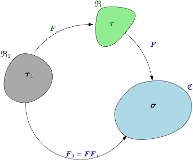
Figure 1: The constitutive relation for the initially stressed configurations $\displaystyle\mathfrak{R}_{1}$ (with initial stress $\displaystyle\boldsymbol{\tau}_{1}$) is known. The goal is to directly determine the response from the reference $\displaystyle\mathfrak{R}$ (with an arbitrary initial stress $\displaystyle\boldsymbol{\tau}$).

The deformation gradients $\displaystyle{\boldsymbol{F}}_{1}$, $\displaystyle{\boldsymbol{F}}$, and $\displaystyle{\boldsymbol{F}}_{0}$ map every infinitesimal vector from $\displaystyle\mathfrak{R}_{1}\to\mathfrak{R}$, $\displaystyle\mathfrak{R}\to\mathfrak{C}$, and $\displaystyle\mathfrak{R}_{1}\to\mathfrak{C}$ respectively, such that $\displaystyle{\boldsymbol{F}}_{0}={\boldsymbol{F}}{\boldsymbol{F}}_{1}$. The constitutive relation (2.2) is known for the reference $\displaystyle\mathfrak{R}_{1}$. We need to determine the constitutive relation for the reference $\displaystyle\mathfrak{R}$ with initial stress $\displaystyle\boldsymbol{\tau}$.

When $\displaystyle\mathfrak{R}_{1}$ is chosen as the reference, the Cauchy stress $\displaystyle\boldsymbol{\sigma}$ is a function of $\displaystyle{\boldsymbol{F}}_{1}$ and $\displaystyle\boldsymbol{\tau}_{1}$. On the other hand, when $\displaystyle\mathfrak{R}$ is the reference, Cauchy stress $\displaystyle\boldsymbol{\sigma}$ will solely be a function of $\displaystyle{\boldsymbol{F}}$ and $\displaystyle\boldsymbol{\tau}$, which is determined in this section. To the best of our knowledge, such a way of changing reference was never adapted earlier.

3.1 Determining a simple form of stress-representation from the stressed reference $\displaystyle\mathfrak{R}$

A simple form of the constitutive relation is chosen for the stressed reference $\displaystyle\mathfrak{R}_{1}$ for which

$${\Psi}_{1}=p_{0},\quad{\Psi}_{2}={\Psi}_{8}={\Psi}_{9}={\Psi}_{10}=0.\quad{\Psi}_{7}=1,$$ (3.1)

in (2.2). When $\displaystyle\Psi_{i}$ remains constant, Eqn. (3.1) satisfies the initial condition (2.3).

Using the material parameter (3.1) in the constitutive relation (2.2) for the reference $\displaystyle\mathfrak{R}_{1}$, the Cauchy stress in the configurations $\displaystyle\mathfrak{C}$ and $\displaystyle\mathfrak{R}$ (see Figure 1) are obtained as

$$\displaystyle\boldsymbol{\sigma} \displaystyle=\Psi_{1}{\boldsymbol{B}}_{0}+{\boldsymbol{F}}_{0}\boldsymbol{\tau}_{1}{\boldsymbol{F}}_{0}^{T}-p{\boldsymbol{I}},$$ (3.2)

$$\displaystyle\boldsymbol{\tau} \displaystyle=\Psi_{1}{\boldsymbol{B}}_{1}+{\boldsymbol{F}}_{1}\boldsymbol{\tau}_{1}{\boldsymbol{F}}_{1}^{T}-{p}_{1}{\boldsymbol{I}},$$ (3.3)

where $\displaystyle p$ and $\displaystyle{p}_{1}$ are the Lagrangian multipliers in $\displaystyle\mathfrak{C}$ and $\displaystyle\mathfrak{R}$ respectively.

The multiplicative decomposition $\displaystyle{\boldsymbol{F}}_{0}={\boldsymbol{F}}{\boldsymbol{F}}_{1}$, and a few simplifications reframe Equation (3.2) as

$$\displaystyle\boldsymbol{\sigma} \displaystyle=\Psi_{1}{\boldsymbol{F}}{\boldsymbol{B}}_{1}{\boldsymbol{F}}^{T}+{\boldsymbol{F}}{\boldsymbol{F}}_{1}\boldsymbol{\tau}_{1}{\boldsymbol{F}}_{1}^{T}{\boldsymbol{F}}^{T}-p{\boldsymbol{I}}$$ (3.4)

$$\displaystyle={\boldsymbol{F}}\left[\Psi_{1}{\boldsymbol{B}}_{1}+{\boldsymbol{F}}_{1}\boldsymbol{\tau}_{1}{\boldsymbol{F}}_{1}^{T}\right]{\boldsymbol{F}}^{T}-p{\boldsymbol{I}}.$$ (3.5)

We can also rewrite Equation (3.3) as

$$\displaystyle\Psi_{1}{\boldsymbol{B}}_{1}+{\boldsymbol{F}}_{1}\boldsymbol{\tau}_{1}{\boldsymbol{F}}_{1}^{T}=\boldsymbol{\tau}+p_{1}{\boldsymbol{I}}.$$ (3.6)

Substitution of (3.6) into the bracketed portion of (3.5) provides

$$\displaystyle\boldsymbol{\sigma}=p_{1}{\boldsymbol{B}}+{\boldsymbol{F}}\tau{\boldsymbol{F}}^{T}-p{\boldsymbol{I}}$$ (3.7)

The constitutive relation (3.7) completely depends on deformation measured from the reference $\displaystyle\mathfrak{R}\rightarrow\mathfrak{C}$ and the initial stress $\displaystyle\boldsymbol{\tau}$ in $\displaystyle\mathfrak{R}$. Hence (3.7) represents the Cauchy stress $\displaystyle\boldsymbol{\sigma}$ from the initially stressed reference $\displaystyle\mathfrak{R}$.

The unknown parameter $\displaystyle p_{1}$ is determined from initial stress $\displaystyle\boldsymbol{\tau}$, by computing the determinants of both the sides of (3.6) as

$$\displaystyle\text{det}\left({\boldsymbol{F}}_{1}\right)\text{det}\left(\Psi_{1}{\boldsymbol{I}}+\boldsymbol{\tau}_{1}\right)\text{det}\left({\boldsymbol{F}}_{1}^{T}\right)=\text{det}\left(\boldsymbol{\tau}+p_{1}{\boldsymbol{I}}\right)$$ (3.8)

The incompressibility condition $\displaystyle\text{det}\left({\boldsymbol{F}}_{1}\right)=1$ simplifies (3.8) as,

$$\displaystyle\text{det}\left(\Psi_{1}{\boldsymbol{I}}+\boldsymbol{\tau}_{1}\right)=\text{det}\left(\boldsymbol{\tau}+p_{1}{\boldsymbol{I}}\right)$$ (3.9)

$$\displaystyle\implies \displaystyle\Psi_{1}^{3}+\Psi_{1}^{2}I_{4}+\Psi_{1}I_{5}+I_{6}=p_{1}^{3}+p_{1}^{2}I_{1_{\tau}}+p_{1}I_{2_{\tau}}+I_{3_{\tau}}$$ (3.10)

where $\displaystyle I_{4}$, $\displaystyle I_{5}$, and $\displaystyle I_{6}$ are the three invariants (2.1) of $\displaystyle\boldsymbol{\tau}_{1}$ and $\displaystyle I_{1_{\tau}}$, $\displaystyle I_{2_{\tau}}$, and $\displaystyle I_{3_{\tau}}$ are the invariants of $\displaystyle\boldsymbol{\tau}$. We can solve Equation (3.10) to determine the parameter $\displaystyle p_{1}$.

Note that. for $\displaystyle\boldsymbol{\tau}={\boldsymbol{Q}}\boldsymbol{\tau}_{1}{\boldsymbol{Q}}^{T}$, where $\displaystyle{\boldsymbol{Q}}$ is a pure rotation, Equation (3.10) yields

$$p_{1}=\Psi_{1}.$$ (3.11)

In this case, the constitutive relation (3.2) for the reference $\displaystyle\mathfrak{R}_{1}$ is also applicable to $\displaystyle\mathfrak{R}$ and vice versa.

Since the reference $\displaystyle\mathfrak{R}$ is subject to an arbitrary initial stress $\displaystyle\boldsymbol{\tau}$. It can be chosen to be $\displaystyle\boldsymbol{\tau}=\bf 0$, for which the solution to Equation (3.10) is

$$\bar{p}=\sqrt[3]{\Psi_{1}^{3}+\Psi_{1}^{2}I_{4}+\Psi_{1}I_{5}+I_{6}},$$ (3.12)

where $\displaystyle p_{1}=\bar{p}$ for $\displaystyle\boldsymbol{\tau}=\bf 0$. For this case, (3.7), reduces to

$$\displaystyle\boldsymbol{\sigma}=\bar{p}{\boldsymbol{B}}-p{\boldsymbol{I}}.$$ (3.13)

which is the response of the stress-free material.

This section provides a direct and easy way to determine the constitutive relation for the arbitray stressed reference $\displaystyle\mathfrak{R}$ and the stress-free reference $\displaystyle\mathfrak{R}_{0}$, which is further generalized in Section 5.

We next focus on our most general approach, for which the constitutive relation becomes implicit by changing the reference configuration.

4 The second approach to determine the response of the stress-free reference $\displaystyle\mathfrak{R}_{0}$ and any arbitrary stressed reference $\displaystyle\mathfrak{R}$

Our first goal in this section is to determine the constitutive response of the stress-free material in Section 4.1, which includes many special cases. In Section 4.2, the constitutive relations of an arbitrary stressed reference $\displaystyle\mathfrak{R}$ is determined in various ways.

The general response in both cases can be implicit, as we find out.

4.1 Identifying the response of the stress-free reference

In this section, we determine the stress-free material response through an in-depth exploration and inversion of a new kind of constitutive relation. In Appendix A, universal relations [15, 16, 17] are established for an implicit constitutive class which helps in simplification

4.1.1 Determining the general implicit constitutive relation for stress-free materials

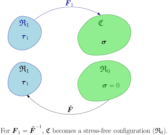
Figure 2: The configurations required in Section 2 and Section 4.1. Top: the deformation gradient $\displaystyle{\boldsymbol{F}}_{1}$ maps a stressed reference $\displaystyle\mathfrak{R}_{1}$ to the current configuration $\displaystyle\mathfrak{C}$, with Cauchy stress $\displaystyle\boldsymbol{\sigma}$. Bottom: the deformation gradient $\displaystyle\hat{{\boldsymbol{F}}}$ maps a vector from the stress-free reference $\displaystyle\mathfrak{R}_{0}$ to initially stressed body $\displaystyle\mathfrak{R}_{1}$. This deformation $\displaystyle\hat{{\boldsymbol{F}}}$ is associated with initial strain/ residual strain. Note: when Cauchy stress $\displaystyle\boldsymbol{\sigma}=0$ in the current configuration $\displaystyle\mathfrak{C}$, it is equivalent to $\displaystyle\mathfrak{R}_{0}$. In this particular case, we have an access the stress-free reference without a destructive testing.

It is not easy to obtain a stress-free material without performing a destructive testing. In this section, we use a thought experiment, demonstrated in Figure 2, to access the stress-free configuration.

Figure 2 (top) shows that a deformation gradient $\displaystyle{\boldsymbol{F}}_{1}$ maps the stressed configuration $\displaystyle\mathfrak{R}_{1}$ to the current configuration $\displaystyle\mathfrak{C}$ with Cauchy stress $\displaystyle\boldsymbol{\sigma}$. The constitutive relation for $\displaystyle\mathfrak{R}_{1}$ is governed by Eqn. (2.2). Our goal is to determine the response of reference $\displaystyle\mathfrak{R}_{0}$.

When $\displaystyle\boldsymbol{\sigma}$ vanishes in the current, $\displaystyle\mathfrak{C}$ represents a stress-free configuration, i.e., $\displaystyle\mathfrak{C}\equiv\mathfrak{R}_{0}$. This provides a way to access the stress-free reference $\displaystyle\mathfrak{R}_{0}$. In this case, we have

$${\boldsymbol{F}}_{1}=\hat{{\boldsymbol{F}}}^{-1},$$ (4.1)

where $\displaystyle\hat{{\boldsymbol{F}}}$ (Figure 2 (bottom)) maps the stress-free configuration $\displaystyle\mathfrak{R}_{0}$ to the stressed reference $\displaystyle\mathfrak{R}_{1}$. This deformation gradient $\displaystyle\hat{{\boldsymbol{F}}}$ is associated with the initial strain in $\displaystyle\mathfrak{R}_{1}$. Eqn. (4.1) further implies

$$\displaystyle{\boldsymbol{C}}_{1}=\hat{{\boldsymbol{B}}}^{-1},\quad{\boldsymbol{B}}_{1}=\hat{{\boldsymbol{C}}}^{-1},$$ (4.2)

where $\displaystyle\hat{{\boldsymbol{B}}}=\hat{{\boldsymbol{F}}}\hat{{\boldsymbol{F}}}^{T}$, $\displaystyle\hat{{\boldsymbol{C}}}=\hat{{\boldsymbol{F}}}^{T}\hat{{\boldsymbol{F}}}$ represent alternative measures of residual strain in the reference $\displaystyle\mathfrak{R}_{1}$, $\displaystyle{\boldsymbol{B}}_{1}={\boldsymbol{F}}_{1}{\boldsymbol{F}}_{1}^{T}$, and $\displaystyle{\boldsymbol{C}}_{1}={\boldsymbol{F}}_{1}^{T}{\boldsymbol{F}}_{1}$.

Note that the stress-free configuration $\displaystyle\mathfrak{R}_{0}$ can undergo any additional arbitrary rotation, and still remains stress-free. Consequently, this configuration is not unique. This non-uniqueness, however does not influence the present investigation as explained in Appendix B.

Substituting equations Eqn. (4.1) and Eqn. (4.2 b) into Eqn. (2.2), and considering that the Cauchy stress vanishes, i.e., $\displaystyle\boldsymbol{\sigma}=\bf 0$, the condition to obtain a stress-free current configuration $\displaystyle\left(\mathfrak{R}_{0}\equiv\mathfrak{C}\right)$ is given by

$$\displaystyle\bf 0 \displaystyle=\bar{\Psi}_{1}\hat{{\boldsymbol{C}}}^{-1}+\bar{\Psi}_{2}\hat{{\boldsymbol{C}}}^{-2}+\bar{\Psi}_{7}\hat{{\boldsymbol{F}}}^{-1}\boldsymbol{\tau}_{1}\hat{{\boldsymbol{F}}}^{-T}+\bar{\Psi}_{8}\left(\hat{{\boldsymbol{F}}}^{-1}\boldsymbol{\tau}_{1}\hat{{\boldsymbol{F}}}^{-T}\hat{{\boldsymbol{C}}}^{-1}+\hat{{\boldsymbol{C}}}^{-1}\hat{{\boldsymbol{F}}}^{-1}\boldsymbol{\tau}_{1}\hat{{\boldsymbol{F}}}^{-T}\right)$$

$$\displaystyle+\bar{\Psi}_{9}\hat{{\boldsymbol{F}}}^{-1}\boldsymbol{\tau}_{1}^{2}\hat{{\boldsymbol{F}}}^{-T}+\bar{\Psi}_{10}\left(\hat{{\boldsymbol{F}}}^{-1}\boldsymbol{\tau}_{1}^{2}\hat{{\boldsymbol{F}}}^{-T}\hat{{\boldsymbol{C}}}^{-1}+\hat{{\boldsymbol{C}}}^{-1}\hat{{\boldsymbol{F}}}^{-1}\boldsymbol{\tau}_{1}^{2}\hat{{\boldsymbol{F}}}^{-T}\right)-\bar{p}{\boldsymbol{I}},$$ (4.3)

$$\displaystyle\text{where }\quad\bar{\Psi}_{i}={\Psi}_{i}\big{|}_{{\boldsymbol{F}}_{1}=\hat{{\boldsymbol{F}}}^{-1}}\quad\text{and}\quad\bar{p}={{p}}\big{|}_{{\boldsymbol{F}}_{1}=\hat{{\boldsymbol{F}}}^{-1}}.$$ (4.4)

Pre-multiplying $\displaystyle\hat{{\boldsymbol{F}}}$ and post-multiplying $\displaystyle\hat{{\boldsymbol{F}}}^{T}$ to both sides of (4.3), we obtain

$$\displaystyle\bf 0 \displaystyle=\bar{\Psi}_{1}{\boldsymbol{I}}+\bar{\Psi}_{2}\hat{{\boldsymbol{B}}}^{-1}+\bar{\Psi}_{7}\boldsymbol{\tau}_{1}+\bar{\Psi}_{8}\left(\boldsymbol{\tau}_{1}\hat{{\boldsymbol{B}}}^{-1}+\hat{{\boldsymbol{B}}}^{-1}\boldsymbol{\tau}_{1}\right)+\bar{\Psi}_{9}\boldsymbol{\tau}_{1}^{2}+\bar{\Psi}_{10}\left(\boldsymbol{\tau}_{1}^{2}\hat{{\boldsymbol{B}}}^{-1}+\hat{{\boldsymbol{B}}}^{-1}\boldsymbol{\tau}_{1}^{2}\right)-\bar{p}\hat{{\boldsymbol{B}}}.$$ (4.5)

Now (see Figure 2 (bottom)), we choose $\displaystyle\mathfrak{R}_{0}$ as the stress-free reference and $\displaystyle\mathfrak{R}_{1}$ as the current configuration. In this case, $\displaystyle\hat{{\boldsymbol{F}}}$, $\displaystyle\hat{{\boldsymbol{B}}}$, and $\displaystyle\boldsymbol{\tau}_{1}$ respectively represent the deformation gradient, the left Cauchy-Green stretch, and the Cauchy stress in the current configuration $\displaystyle\mathfrak{R}_{1}$. Altogether, Equation (4.5) represents the constitutive relation for the stress-free reference $\displaystyle\mathfrak{R}_{0}$, which involves the Cauchy stress $\displaystyle\boldsymbol{\tau}_{1}$ and the left Cauchy stretch $\displaystyle\hat{{\boldsymbol{B}}}$. Very interestingly, this general constitutive relation (4.5) is implicit by nature which is equivalent to, and bears considerable similarity with the standard form of implicit constitutive relation [10, 9, 13, 39].

The constitutive relation (4.5) clearly shows that the stress-free reference $\displaystyle\mathfrak{R}_{0}$ is isotropic. We further establish the universal relations for these general implicit elastic materials in Appendix A, which incidentally simplifies (4.5). It is noted that Rajagopal and Wineman [17] have developed universal relation for another class of implicit elasticity. Using the universal relations (Appendix A), we have

$$\hat{{\boldsymbol{B}}}^{-1}\boldsymbol{\tau}_{1}=\boldsymbol{\tau}_{1}\hat{{\boldsymbol{B}}}^{-1},\quad\hat{{\boldsymbol{B}}}^{-1}\boldsymbol{\tau}_{1}^{2}=\boldsymbol{\tau}_{1}^{2}\hat{{\boldsymbol{B}}}^{-1}.$$ (4.6)

Use of Eqn. (4.6) further simplifies (4.5) as

$$\displaystyle\bf 0 \displaystyle=\left(\bar{\Psi}_{1}{\boldsymbol{I}}+\bar{\Psi}_{7}\boldsymbol{\tau}_{1}+\bar{\Psi}_{9}\boldsymbol{\tau}_{1}^{2}\right){\boldsymbol{I}}-\bar{p}\hat{{\boldsymbol{B}}}+\left(\bar{\Psi}_{2}{\boldsymbol{I}}+2\bar{\Psi}_{8}\boldsymbol{\tau}_{1}+2\bar{\Psi}_{10}\boldsymbol{\tau}_{1}^{2}\right)\hat{{\boldsymbol{B}}}^{-1},\text{ or}$$ (4.7)

$$\displaystyle\bf 0 \displaystyle=\left(\bar{\Psi}_{1}{\boldsymbol{I}}-\bar{p}\hat{{\boldsymbol{B}}}+\bar{\Psi}_{2}\hat{{\boldsymbol{B}}}^{-1}\right){{\boldsymbol{I}}}+\left(\bar{\Psi}_{7}{\boldsymbol{I}}+2\bar{\Psi}_{8}\hat{{\boldsymbol{B}}}^{-1}\right){\boldsymbol{\tau}_{1}}+\left(2\bar{\Psi}_{10}{\boldsymbol{I}}+\bar{\Psi}_{9}\hat{{\boldsymbol{B}}}\right){\boldsymbol{\tau}_{1}^{2}}\$$ (4.8)

It is noted that when $\displaystyle\bar{\Psi}_{i}\left({\boldsymbol{X}}_{1}\right)$ are independent of $\displaystyle\boldsymbol{\tau}_{1}$ or $\displaystyle\hat{{\boldsymbol{F}}}_{1}$, we have

$${\Psi}_{i}\left({\boldsymbol{X}}_{1}\right)=\bar{\Psi}_{i}\left({\boldsymbol{X}}_{1}\right)={\Psi}_{i_{0}}\left({\boldsymbol{X}}_{1}\right).$$ (4.9)

(Also see Eqn. 4.4, and Eqn. 2.3.)

Equation (4.7, 4.8) represent the general implicit constitutive relation between the Cauchy stress $\displaystyle\boldsymbol{\tau}_{1}$ and the left Cauchy stretch $\displaystyle\hat{{\boldsymbol{B}}}$ for the stress-free reference $\displaystyle\mathfrak{R}_{0}$. All these constitutive relations are implicit, represented in a slightly different form.

We also determine two special explicit form of this constitutive relation for the stress-free reference $\displaystyle\mathfrak{R}_{0}$ in Section 4.1.2 and Section 4.1.3, respectively.

4.1.2 Special case-I

In this section, we consider the special case

$$\bar{\Psi}_{1}=p_{0},\quad\bar{\Psi}_{2}=\bar{\Psi}_{8}=\bar{\Psi}_{9}=\bar{\Psi}_{10}=0.\quad\bar{\Psi}_{7}=1,$$ (4.10)

to determine the explicit response of the stress-free material. For this choice, the implicit constitutive relation (4.7) for the stress-free reference $\displaystyle\mathfrak{R}_{0}$ reduces to

$$\boldsymbol{\tau}_{1}=\bar{p}\hat{{\boldsymbol{B}}}-\bar{\psi}_{1}{\boldsymbol{I}}=\bar{p}\hat{{\boldsymbol{B}}}-p_{0}{\boldsymbol{I}}.$$ (4.11)

(Since we consider that constitutive relation depends on reference, only Eqn. (4.5) applies to the reference $\displaystyle\mathfrak{R}_{0}$, not Eqn. (2.2).) Note that the parameter $\displaystyle p_{0}=\bar{\Psi}_{1}$ appears to the Lagrange multiplier of incompressibility when the stress-free configuration $\displaystyle\mathfrak{R}_{0}$ is used as the reference and $\displaystyle\mathfrak{R}_{1}$ as the current.

We further invert (4.11) to determine the initial strain $\displaystyle\hat{{\boldsymbol{B}}}$ in $\displaystyle\mathfrak{R}_{1}$ as

$$\hat{{\boldsymbol{B}}}=\frac{1}{\bar{p}}\boldsymbol{\tau}_{1}+\frac{p_{0}}{\bar{p}}{\boldsymbol{I}}.$$ (4.12)

The parameter $\displaystyle\bar{p}$ here is obtained by equating the determinant of both the sides of (4.12) to unity (due to incompressibility) as follows

$$\bar{p}=\sqrt[3]{\text{det}\left[\boldsymbol{\tau}_{1}+\bar{\Psi}_{1}{\boldsymbol{I}}\right]}.$$ (4.13)

We recall that the constitutive relation (4.11) is applicable when $\displaystyle\mathfrak{R}_{0}$ is chosen as the reference and $\displaystyle\mathfrak{R}_{1}$ as the current configuration. Extending (4.11), the general constitutive relation for the stress-free reference $\displaystyle\mathfrak{R}_{0}$ and a current configuration $\displaystyle\mathfrak{C}_{1}$ (see Figure 4) is obtained as

$$\boldsymbol{\sigma}=\bar{p}{{\boldsymbol{B}}}_{tot}-p{\boldsymbol{I}}.$$ (4.14)

where $\displaystyle{\boldsymbol{B}}_{tot}={\boldsymbol{F}}_{tot}{\boldsymbol{F}}_{tot}^{T}$, $\displaystyle{\boldsymbol{F}}_{tot}$ maps any vector from $\displaystyle\mathfrak{R}_{0}$ to a current configuration $\displaystyle\mathfrak{C}_{1}$.

Note that a new deformation gradient $\displaystyle{\boldsymbol{F}}_{tot}$ and new current configuration $\displaystyle\mathfrak{C}_{1}$ are introduced at this point. Once, we know the response of the stress-free reference, the reference $\displaystyle\mathfrak{R}_{1}$ is not needed to further change the reference configuration. We use the constitutive relation (4.14) for $\displaystyle\mathfrak{R}_{0}$ to determine the response of an arbitrary initial stressed reference $\displaystyle\mathfrak{R}$ (in Section 4.2.2).

4.1.3 Special case-II

Here we consider the special case:

$$\bar{\Psi}_{2}=p_{0},\quad\bar{\Psi}_{1}=\bar{\Psi}_{7}=\bar{\Psi}_{9}=\bar{\Psi}_{10}=0,\quad\bar{\Psi}_{8}=\frac{1}{2},$$ (4.15)

for which the constitutive relation (4.5):

$$\displaystyle\bf 0 \displaystyle=\bar{\Psi}_{2}\hat{{\boldsymbol{B}}}^{-1}+\bar{\Psi}_{8}\left(\boldsymbol{\tau}_{1}\hat{{\boldsymbol{B}}}^{-1}+\hat{{\boldsymbol{B}}}^{-1}\boldsymbol{\tau}_{1}\right)-\bar{p}\hat{{\boldsymbol{B}}}.$$ (4.16)

can be simplified into

$$\displaystyle\boldsymbol{\tau}_{1} \displaystyle=\frac{\bar{p}}{2\bar{\Psi}_{8}}\hat{{\boldsymbol{B}}}^{2}-\frac{\bar{\Psi}_{2}}{2\bar{\Psi}_{8}}{\boldsymbol{I}},$$ (4.17)

either through a few intermediate steps, or by directly substituting Eqn. (4.15) into Eqn. (4.7).

In the constitutive relation (4.17), $\displaystyle\tfrac{\bar{\Psi}_{2}}{2\bar{\Psi}_{8}}$ acts as the Lagrange multiplier, when we consider $\displaystyle\mathfrak{R}_{0}$ as the reference and $\displaystyle\mathfrak{R}_{1}$ as the current. Consequently, the initial strain in $\displaystyle\mathfrak{R}_{1}$ is evaluated as

$$\displaystyle\hat{{\boldsymbol{B}}}=\sqrt{\left(\frac{2\bar{\Psi}_{8}}{\bar{p}}\boldsymbol{\tau}_{1}+\frac{\bar{\Psi}_{2}}{\bar{p}}{\boldsymbol{I}}\right)},$$ (4.18)

and $\displaystyle\bar{p}$ can be determined as

$$\bar{p}=\sqrt[3]{\text{det}\left[2\bar{\Psi}_{8}\boldsymbol{\tau}_{1}+\bar{\Psi}_{2}{\boldsymbol{I}}\right]}.$$ (4.19)

from the incompressibility condition $\displaystyle\text{det}\hat{{\boldsymbol{B}}}=1$.

By extending (4.17), the general constitutive relation for the stress-free reference $\displaystyle\mathfrak{R}_{0}$ and current configuration $\displaystyle\mathfrak{C}_{1}$ (in Figure 4) is obtained as

$$\boldsymbol{\sigma}=\frac{\bar{p}}{2\bar{\Psi}_{8}}{{\boldsymbol{B}}}^{2}_{tot}-p{\boldsymbol{I}}.$$ (4.20)

where $\displaystyle{\boldsymbol{B}}_{tot}={\boldsymbol{F}}_{tot}{\boldsymbol{F}}_{tot}^{T}$, $\displaystyle{\boldsymbol{F}}_{tot}$ (see Figure 4) maps an infinitesimal vector from $\displaystyle\mathfrak{R}_{0}$ to a current configuration $\displaystyle\mathfrak{C}_{1}$. We use this relation to determine the response of the initially stressed reference $\displaystyle\mathfrak{R}$ in Section 4.2.3

4.2 The response of any arbitrary stressed reference $\displaystyle\mathfrak{R}$

In this section, our goal is to determine the response of any arbitrarily stressed reference $\displaystyle\mathfrak{R}$ with initial stress $\displaystyle\boldsymbol{\tau}$.

4.2.1 An implicit constitutive relation for the stressed reference $\displaystyle\mathfrak{R}$

In contrast with the approach of Section 4.1.1, here we consider that the current configuration $\displaystyle\mathfrak{C}$ is not stress-free. The Cauchy stress in $\displaystyle\mathfrak{C}$ is given by $\displaystyle\boldsymbol{\tau}$, such that we have $\displaystyle\mathfrak{C}\equiv\mathfrak{R}$. This set up is schematically shown in Fig. 3 (top). By choosing $\displaystyle\mathfrak{R}_{1}$ as the reference and $\displaystyle\mathfrak{R}$ as the current, where the constitutive relation Eqn. (2.2) is applicable, the Cauchy stress $\displaystyle\boldsymbol{\tau}$ in the current configuration is given by

$$\displaystyle\boldsymbol{\tau} \displaystyle=\Psi_{1}{\boldsymbol{B}}_{1}+\Psi_{2}{\boldsymbol{B}}_{1}^{2}+\Psi_{7}{\boldsymbol{F}}_{1}\boldsymbol{\tau}_{1}{\boldsymbol{F}}_{1}^{T}+\Psi_{8}\left({\boldsymbol{F}}_{1}\boldsymbol{\tau}_{1}{\boldsymbol{F}}_{!}^{T}{\boldsymbol{B}}_{1}+{\boldsymbol{B}}_{1}{\boldsymbol{F}}_{1}\boldsymbol{\tau}_{1}{\boldsymbol{F}}_{1}^{T}\right)$$

$$\displaystyle+\Psi_{9}{\boldsymbol{F}}_{1}\boldsymbol{\tau}_{1}^{2}{\boldsymbol{F}}_{1}^{T}+\Psi_{10}\left({\boldsymbol{F}}_{1}\boldsymbol{\tau}_{1}^{2}{\boldsymbol{F}}_{1}^{T}{\boldsymbol{B}}_{1}+{\boldsymbol{B}}_{1}{\boldsymbol{F}}_{1}\boldsymbol{\tau}_{1}^{2}{\boldsymbol{F}}_{1}^{T}\right)-p{\boldsymbol{I}}.$$ (4.21)

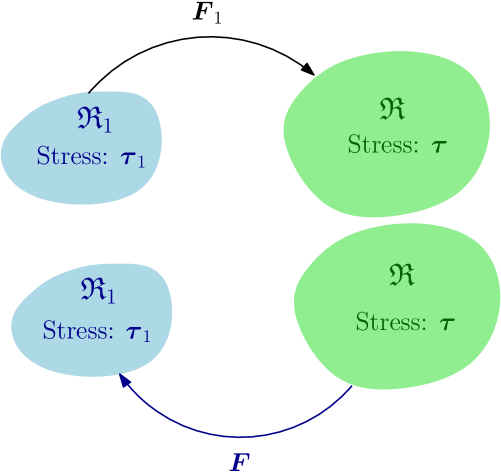
Figure 3: The problem set up for Section 4.2.1. Top: we choose $\displaystyle\mathfrak{R}_{1}$ as the reference, and $\displaystyle\mathfrak{R}$ as the current, where the deformation gradient is $\displaystyle{\boldsymbol{F}}_{1}$. Bottom: $\displaystyle\mathfrak{R}$ is chosen as the reference and $\displaystyle\mathfrak{R}_{1}$ as the current, with deformation gradient $\displaystyle{\boldsymbol{F}}={\boldsymbol{F}}_{1}^{-1}$. The constitutive relation is known for the case at the Top and determined for the case at the Bottom.

As shown in Figure 3 (bottom), we next consider $\displaystyle\mathfrak{R}$ as the initially stressed reference and $\displaystyle\mathfrak{R}_{1}$ as the current, where the Cauchy stress is $\displaystyle\boldsymbol{\tau}_{1}$ and determine the constitutive relation. In this section, the deformation gradient from $\displaystyle\mathfrak{R}$ to $\displaystyle\mathfrak{R}_{1}$ is denoted by $\displaystyle{\boldsymbol{F}}$.

We substitute $\displaystyle{\boldsymbol{F}}_{1}={\boldsymbol{F}}^{-1}$ and $\displaystyle{\boldsymbol{B}}_{1}={\boldsymbol{C}}^{-1}$ into Eqn. (4.21), pre-multiply the resulting equation with $\displaystyle{{\boldsymbol{F}}}$, and post-multiply the same with $\displaystyle{{\boldsymbol{F}}}^{T}$, to obtain

$$\displaystyle 0 \displaystyle=\bar{\Psi}_{1}{\boldsymbol{I}}+\bar{\Psi}_{2}{{\boldsymbol{B}}}^{-1}+\bar{\Psi}_{7}\boldsymbol{\tau}_{1}+\bar{\Psi}_{8}\left(\boldsymbol{\tau}_{1}{{\boldsymbol{B}}}^{-1}+{{\boldsymbol{B}}}^{-1}\boldsymbol{\tau}_{1}\right)+\bar{\Psi}_{9}\boldsymbol{\tau}_{1}^{2}+\bar{\Psi}_{10}\left(\boldsymbol{\tau}_{1}^{2}{{\boldsymbol{B}}}^{-1}+{{\boldsymbol{B}}}^{-1}\boldsymbol{\tau}_{1}^{2}\right)-{{\boldsymbol{F}}}\boldsymbol{\tau}{{\boldsymbol{F}}}^{T}-\bar{p}{{\boldsymbol{B}}}.$$ (4.22)

Eqn. (4.22) is the implicit constitutive relation for the arbitrary stressed reference $\displaystyle\mathfrak{R}$ (with initial stress $\displaystyle\boldsymbol{\tau}$), with $\displaystyle\mathfrak{R_{1}}$ as the current configuration (with Cauchy stress $\displaystyle\boldsymbol{\tau}_{1}$).

Mukherjee [41] has developed an implicit elastic framework for initially stressed materials. The present constitutive relation Eqn. (4.22) belongs to the general form Eqn. (2.2) of [41]. However, they have not developed any constitutive relation of the present form by changing the reference configuration.

Please also note that the present constitutive relation Eqn (4.22) is not determined using a virtual stress-free configuration.

Since, we have determined the explicit response for the stress-free reference in Section 4.1.2 and Section 4.1.3, respectively, we next use them to find out the constitutive relation of $\displaystyle\mathfrak{R}$ in the approach of Johnson, Hoger [1, 2], and Saravanan [3, 42]. The configuration $\displaystyle\mathfrak{R}_{1}$ is no longer necessary to this end. A new current configuration $\displaystyle\mathfrak{C}_{1}$ is introduced in Figure 4.

4.2.2 A Green elastic constitutive relation for the stressed reference $\displaystyle\mathfrak{R}$

When the stress-free configuration $\displaystyle\mathfrak{R}_{0}$ is governed by the constitutive relation (4.14) (Section 4.1.2), we determine here the constitutive relation for the initially stressed reference $\displaystyle\mathfrak{R}$.

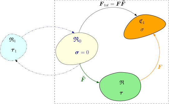
Figure 4: Using the response of stress-free reference $\displaystyle\mathfrak{R}_{0}$, calculated in Section 4.1.2 and 4.1.3, we obtain the constitutive relation for an arbitrarily stressed reference $\displaystyle\mathfrak{R}$ (Section 4.2.2 and 4.2.3). The configuration $\displaystyle R_{1}$ is not used in here any more. Note the multiplicative decomposition of the deformation gradient $\displaystyle\boldsymbol{F}_{0}=\boldsymbol{\tilde{F}}{\boldsymbol{F}}$.

Figure 4 describes the stress-free configuration $\displaystyle\mathfrak{R}_{0}$, initially stressed reference $\displaystyle\mathfrak{R}$, and the current configuration $\displaystyle\mathfrak{C}_{1}$. The deformation gradient from $\displaystyle\mathfrak{R}_{0}\rightarrow\mathfrak{R}$ is $\displaystyle\tilde{{\boldsymbol{F}}}$, from $\displaystyle\mathfrak{R}\rightarrow\mathfrak{C}_{1}$ is $\displaystyle{\boldsymbol{F}}$, and from $\displaystyle\mathfrak{R}_{0}\rightarrow\mathfrak{C}_{1}$ is given by $\displaystyle{\boldsymbol{F}}_{tot}={\boldsymbol{F}}\tilde{{\boldsymbol{F}}}$.

Applying the constitutive relation (4.14) for the reference $\displaystyle\mathfrak{R}_{0}$, while the current configuration is chosen respectively as $\displaystyle\mathfrak{R}$ and $\displaystyle\mathfrak{C}_{1}$, we obtain

$$\displaystyle\boldsymbol{\tau} \displaystyle=\bar{p}\boldsymbol{\tilde{B}}-\tilde{p}{\boldsymbol{I}},$$ (4.23)

$$\displaystyle\boldsymbol{\sigma} \displaystyle=\bar{p}{\boldsymbol{F}}_{tot}{\boldsymbol{F}}_{tot}^{T}-p{\boldsymbol{I}}=\bar{p}{\boldsymbol{F}}\boldsymbol{\tilde{B}}{\boldsymbol{F}}^{T}-p{\boldsymbol{I}},$$ (4.24)

where the multiplicative decomposition $\displaystyle{\boldsymbol{F}}_{tot}={\boldsymbol{F}}\tilde{{\boldsymbol{F}}}$ is used. Eqn. (4.23) can also be alternatively expressed as

$$\bar{p}\boldsymbol{\tilde{B}}=\boldsymbol{\tau}+\tilde{p}{\boldsymbol{I}}.$$ (4.25)

The unknown residual strain $\displaystyle\boldsymbol{\tilde{B}}=\boldsymbol{\tilde{F}}\boldsymbol{\tilde{F}}^{T}$ in (4.24) can be eliminated by substituting Eqn. (4.25) into Eqn. (4.24) to obtain

$$\boldsymbol{\sigma}={\boldsymbol{F}}\boldsymbol{\tau}{\boldsymbol{F}}^{T}+\tilde{p}{\boldsymbol{B}}-p{\boldsymbol{I}}.$$ (4.26)

The constitutive relation (4.26) depends on the the initial stress $\displaystyle\boldsymbol{\tau}$ in the reference $\displaystyle\mathfrak{R}$, and on the deformation gradient $\displaystyle{\boldsymbol{F}}$ from $\displaystyle\mathfrak{R}$ to $\displaystyle\mathfrak{C}_{1}$. Hence, it represents the constitutive relation for the arbitrary stressed reference $\displaystyle\mathfrak{R}$. The unknown parameter $\displaystyle\tilde{p}$ is determined in terms of $\displaystyle\boldsymbol{\tau}$ as follows. Calculating the determinant on both the sides of (4.25) and substituting the incompressibility condition $\displaystyle\text{det}\tilde{{\boldsymbol{B}}}=1$, we obtain

$$\bar{p}^{3}=\text{det}\left(\boldsymbol{\tau}+\tilde{p}{\boldsymbol{I}}\right),$$ (4.27)

which can be solved for $\displaystyle\tilde{p}$, once $\displaystyle\bar{p}$ is obtained from Equation (4.12).

4.2.3 Another Green elastic constitutive relation for the stressed reference $\displaystyle\mathfrak{R}$

When the stress-free material $\displaystyle\mathfrak{R}_{0}$ follows the constitutive relation Eqn. (4.20) (Section 4.1.3), we determine the response of the reference $\displaystyle\mathfrak{R}$ with initial stress $\displaystyle\boldsymbol{\tau}$ (Figure 4).

Substituting $\displaystyle{\boldsymbol{F}}_{tot}={\boldsymbol{F}}\tilde{{\boldsymbol{F}}}$ into Eqn. (4.20) with simplifications, we obtain

$$\boldsymbol{\sigma}=\frac{\bar{p}}{2\bar{\Psi}_{8}}{\boldsymbol{F}}\tilde{{\boldsymbol{B}}}{\boldsymbol{C}}\tilde{{\boldsymbol{B}}}\tilde{{\boldsymbol{F}}}^{T}-p{\boldsymbol{I}}.$$ (4.28)

Considering $\displaystyle\mathfrak{R}_{0}$ as the reference and $\displaystyle\mathfrak{R}$ as the current (see Figure 4), we have

$$\boldsymbol{\tau}=\frac{\bar{p}}{2\bar{\Psi}_{8}}{\tilde{{\boldsymbol{B}}}}^{2}-\tilde{p}{\boldsymbol{I}},$$ (4.29)

where $\displaystyle\tilde{p}$ is the Lagrange multiplier for the configuration $\displaystyle\mathfrak{R}$.

Eqn. (4.29) can be inverted as

$$\tilde{{\boldsymbol{B}}}=\sqrt{\left(\frac{2\bar{\Psi}_{8}}{\bar{p}}\boldsymbol{\tau}+\frac{2\bar{\Psi}_{8}\tilde{p}}{\bar{p}}{\boldsymbol{I}}\right)}$$ (4.30)

We can substitute Eqn. (4.30) into Eqn. (4.29) to determine the representation of Cauchy stress from an arbitrary stressed reference $\displaystyle\mathfrak{R}$. The Lagrange multiplier $\displaystyle\tilde{p}$ is evaluated by applying the incompressibility condition $\displaystyle\text{det}\tilde{{\boldsymbol{B}}}=1$ into Eqn. (4.30), after calculating $\displaystyle\bar{p}$ from Eqn. (4.19).

This section considers an explicit constitutive relation for a given initially stressed reference $\displaystyle\mathfrak{R}_{1}$ and observes that the general constitutive relation for the stress-free reference $\displaystyle\mathfrak{R}_{0}$, or another initially stressed reference $\displaystyle\mathfrak{R}$ can be implicit. This demonstrates the importance and generality of the implicit elasticity [10, 9, 43, 13]

For two specific cases, the explicit constitutive relations are determined for a stress-free reference $\displaystyle\mathfrak{R}_{0}$ and that of any arbitrary initially stressed reference $\displaystyle\mathfrak{R}$.

5 The third approach to determine the response of the stress-free reference $\displaystyle\mathfrak{R}_{0}$ and any arbitrary stressed reference $\displaystyle\mathfrak{R}$

The previous approach presented in Section 4 offers a very general method to change the reference configuration from one initially stressed state to another. The first approach (Section 3), on the other hand, is simple to understand and to apply. In Section 5.1, we show that it may not be easy to employ the second approach when the reference $\displaystyle\mathfrak{R}_{1}$ is governed by a more general constitutive relation, Eqn. (2.2). Hence, in Section 5.2, we extend the second approach for handling the more general cases– to determine more general constitutive relations for the stressed reference $\displaystyle\mathfrak{R}$.

5.1 The difficulty of extending the previous approach to more general cases

We applied the approach of Section 3 when the reference $\displaystyle\mathfrak{R}_{1}$ follows a relatively simpler constitutive relation Eqn. (3.2). When the constitutive relation for reference $\displaystyle\mathfrak{R}_{1}$ has a more general and intricate form Eqn. (2.2), the Cauchy stress in the configurations $\displaystyle\mathfrak{C}$ and $\displaystyle\mathfrak{R}$ (Figure 1) are calculated as

$$\displaystyle\boldsymbol{\sigma} \displaystyle=\Psi_{1}{\boldsymbol{B}}_{0}+\Psi_{2}{\boldsymbol{B}}_{0}^{2}+\Psi_{7}{\boldsymbol{F}}_{0}\boldsymbol{\tau}_{1}{\boldsymbol{F}}_{0}^{T}+\Psi_{8}\left({\boldsymbol{F}}_{0}\boldsymbol{\tau}_{1}{\boldsymbol{F}}_{0}^{T}{\boldsymbol{B}}_{0}+{\boldsymbol{B}}_{0}{\boldsymbol{F}}_{0}\boldsymbol{\tau}_{1}{\boldsymbol{F}}_{0}^{T}\right)$$

$$\displaystyle+\Psi_{9}{\boldsymbol{F}}_{0}\boldsymbol{\tau}_{1}^{2}{\boldsymbol{F}}_{0}^{T}+\Psi_{10}\left({\boldsymbol{F}}_{0}\boldsymbol{\tau}_{1}^{2}{\boldsymbol{F}}_{0}^{T}{\boldsymbol{B}}_{0}+{\boldsymbol{B}}_{0}{\boldsymbol{F}}_{0}\boldsymbol{\tau}_{1}^{2}{\boldsymbol{F}}_{0}^{T}\right)-p{\boldsymbol{I}}$$ (5.1)

$$\displaystyle\boldsymbol{\tau} \displaystyle=\Psi_{1}{\boldsymbol{B}}_{1}+\Psi_{2}{\boldsymbol{B}}_{1}^{2}+\Psi_{7}{\boldsymbol{F}}_{1}\boldsymbol{\tau}_{1}{\boldsymbol{F}}_{1}^{T}+\Psi_{8}\left({\boldsymbol{F}}_{1}\boldsymbol{\tau}_{1}{\boldsymbol{F}}_{1}^{T}{\boldsymbol{B}}_{1}+{\boldsymbol{B}}_{1}{\boldsymbol{F}}_{1}\boldsymbol{\tau}_{1}{\boldsymbol{F}}_{1}^{T}\right)$$

$$\displaystyle+\Psi_{9}{\boldsymbol{F}}_{1}\boldsymbol{\tau}_{1}^{2}{\boldsymbol{F}}_{1}^{T}+\Psi_{10}\left({\boldsymbol{F}}_{1}\boldsymbol{\tau}_{1}^{2}{\boldsymbol{F}}_{1}^{T}{\boldsymbol{B}}_{1}+{\boldsymbol{B}}_{1}{\boldsymbol{F}}_{1}\boldsymbol{\tau}_{1}^{2}{\boldsymbol{F}}_{1}^{T}\right)-p_{1}{\boldsymbol{I}},$$ (5.2)

The equations Eqn. (5.1) and Eqn. (5.2) are similar to the equations Eqn. (3.2) and Eqn. (3.3), respectively. Further substituting the kinematic relations: $\displaystyle{\boldsymbol{F}}_{0}={\boldsymbol{F}}{\boldsymbol{F}}_{1}$, $\displaystyle{\boldsymbol{B}}_{0}={\boldsymbol{F}}{\boldsymbol{B}}_{1}{\boldsymbol{F}}^{T},$ and $\displaystyle{\boldsymbol{B}}_{0}^{2}={\boldsymbol{F}}{\boldsymbol{B}}_{1}{\boldsymbol{C}}{\boldsymbol{B}}_{1}{\boldsymbol{F}}^{T}$ into Eqn. (5.1), we obtain

$$\displaystyle\boldsymbol{\sigma} \displaystyle=\Psi_{1}{\boldsymbol{F}}{\boldsymbol{B}}_{1}{\boldsymbol{F}}^{T}+\Psi_{2}{\boldsymbol{F}}{\boldsymbol{B}}_{1}{\boldsymbol{C}}{\boldsymbol{B}}_{1}{\boldsymbol{F}}^{T}+\Psi_{7}{\boldsymbol{F}}{\boldsymbol{F}}_{1}\boldsymbol{\tau}_{1}{\boldsymbol{F}}_{1}^{T}{\boldsymbol{F}}^{T}$$

$$\displaystyle+\Psi_{8}\left({\boldsymbol{F}}{\boldsymbol{F}}_{1}\boldsymbol{\tau}_{1}{\boldsymbol{F}}_{1}^{T}{\boldsymbol{C}}{\boldsymbol{B}}_{1}{\boldsymbol{F}}^{T}+{\boldsymbol{F}}{\boldsymbol{B}}_{1}{\boldsymbol{C}}{\boldsymbol{F}}_{1}\boldsymbol{\tau}_{1}{\boldsymbol{F}}_{1}^{T}{\boldsymbol{F}}\right)+\Psi_{9}{\boldsymbol{F}}{\boldsymbol{F}}_{1}\boldsymbol{\tau}_{1}^{2}{\boldsymbol{F}}_{1}^{T}{\boldsymbol{F}}^{T}$$

$$\displaystyle+\Psi_{10}\left({\boldsymbol{F}}{\boldsymbol{F}}_{1}\boldsymbol{\tau}_{1}^{2}{\boldsymbol{F}}_{1}^{T}{\boldsymbol{C}}{\boldsymbol{B}}_{1}{\boldsymbol{F}}^{T}+{\boldsymbol{F}}{\boldsymbol{B}}_{1}{\boldsymbol{C}}{\boldsymbol{F}}_{1}\boldsymbol{\tau}_{1}^{2}{\boldsymbol{F}}_{1}^{T}{\boldsymbol{F}}\right)-p{\boldsymbol{I}},$$ (5.3)

which has a form similar to Eqn. (3.4). To obtain the representation of stress $\displaystyle\boldsymbol{\sigma}$ from reference $\displaystyle\mathfrak{R}$, we need to express $\displaystyle\boldsymbol{\sigma}$ solely as a function of $\displaystyle{\boldsymbol{F}}$ and $\displaystyle\boldsymbol{\tau}$ (see Figure 1).

However, unlike the case of Eqn. (3.4), it is more difficult to directly eliminate the initial strain dependent terms $\displaystyle{\boldsymbol{B}}_{1}$, $\displaystyle{\boldsymbol{F}}_{1}\boldsymbol{\tau}_{1}{\boldsymbol{F}}_{1}^{T}$, and $\displaystyle{\boldsymbol{F}}_{1}\boldsymbol{\tau}_{1}^{2}{\boldsymbol{F}}_{1}^{T}$ from Eqn. (5.3).

The other option is to determine $\displaystyle{\boldsymbol{F}}_{1}$ from Eqn. (5.2) which is to be substituted in Eqn. (5.3) to eliminate $\displaystyle{\boldsymbol{F}}_{1}$ completely. However, we are not able to determine $\displaystyle{\boldsymbol{F}}_{1}$ from Eqn. (5.2), since $\displaystyle{\boldsymbol{F}}_{1}$ has $\displaystyle 9$ independent components, and Eqn. (5.2) represents $\displaystyle 6$ simultaneous equations in three dimensions. The $\displaystyle 3$ additional components appears due to the rotation part of $\displaystyle{\boldsymbol{F}}_{1}$, which is not unique. In Section 5.2, we present an approach where only $\displaystyle 6$ unknown initial strain components are determined from a set of $\displaystyle 6$ equations, to eliminate initial strain.

5.2 The more general approach

To avoid the above difficulties associated with the non-unique rotation part of $\displaystyle{\boldsymbol{F}}_{1}$ (Section 5.1), we bring in an imaginary stressed reference $\displaystyle\mathfrak{R}_{1}^{\prime}$ in such a way that there remain only $\displaystyle 6$ unknown components of the deformation gradient $\displaystyle{\boldsymbol{F}}_{1}$, and the non-unique rotation is eliminated.

We can better visualize this approach (see Figure 5) by diagonalizing $\displaystyle\boldsymbol{\tau}$ and $\displaystyle\boldsymbol{\tau}_{1}$ as

$$\displaystyle\boldsymbol{\tau}_{1}=\sum_{i}\tau_{1_{i}}{{\boldsymbol{E}}_{1}}_{i}\otimes{{\boldsymbol{E}}_{1}}_{i} \displaystyle\boldsymbol{\tau}=\sum_{i}\tau_{i}{{\boldsymbol{E}}}_{i}\otimes{{\boldsymbol{E}}}_{i},$$ (5.4)

where $\displaystyle{{\boldsymbol{E}}_{1}}_{i}$, $\displaystyle{\boldsymbol{E}}_{i}$ are the eigenvectors, and $\displaystyle\tau_{1_{i}}$, $\displaystyle\tau_{i}$ are the eigenvalues of the initial stress $\displaystyle\boldsymbol{\tau}_{1}$ and $\displaystyle\boldsymbol{\tau}$ respectively.

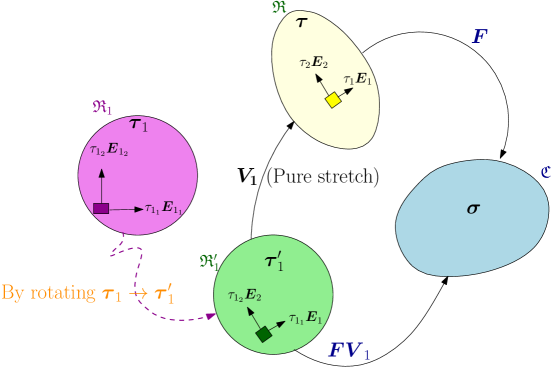
Figure 5: The general approach of Section 5. The initial stress $\displaystyle\boldsymbol{\tau}_{1}$ in $\displaystyle\mathfrak{R}_{1}$ is rotated to $\displaystyle\boldsymbol{\tau}_{1}^{\prime}={\boldsymbol{Q}}\boldsymbol{\tau}_{1}{\boldsymbol{Q}}^{T}$ to form an imaginary initially stressed configuration $\displaystyle\mathfrak{R}_{1}^{\prime}$, such that the stress $\displaystyle\boldsymbol{\tau}_{1}^{\prime}$ becomes coaxial with $\displaystyle\boldsymbol{\tau}$ in $\displaystyle\mathfrak{R}$. With this co-axiality, since the stress-free material is isotropic, the deformation from $\displaystyle\mathfrak{R}_{1}^{\prime}$ to $\displaystyle\mathfrak{R}$ has to be a pure stretch $\displaystyle{\boldsymbol{V}}_{1}$, which is coaxial with both $\displaystyle\boldsymbol{\tau}_{1}^{\prime}$ and $\displaystyle\boldsymbol{\tau}$. This pure stretch is determined by inverting constitutive relation for the reference $\displaystyle\mathfrak{R}_{1}^{\prime}$. Since $\displaystyle\mathfrak{R}_{1}^{\prime}$ is an imaginary configuration, which can not and need not be physically accessed, there is no requirement for the stress-field $\displaystyle\boldsymbol{\tau}_{1}^{\prime}$ to be self-balancing. Only the kinematic relations and constitutive relation are necessary here.

The imaginary stressed reference $\displaystyle\mathfrak{R}^{\prime}_{1}$ (see Figure 5) is subject to an initial stress

$$\boldsymbol{\tau}_{1}^{\prime}=\sum_{i}\tau_{1_{i}}{{\boldsymbol{E}}}_{i}\otimes{{\boldsymbol{E}}}_{i},$$ (5.5)

whose principal directions align with the eigenvectors of $\displaystyle\boldsymbol{\tau}$, and the principal values are the same as the eigenvalues of $\displaystyle\boldsymbol{\tau}_{1}$, such that

$$\boldsymbol{\tau}_{1}^{\prime}={\boldsymbol{Q}}\boldsymbol{\tau}_{1}{\boldsymbol{Q}}^{T}\text{ where }{\boldsymbol{Q}}=\sum_{i}{{\boldsymbol{E}}_{i}\otimes{\boldsymbol{E}}_{1_{i}}}.$$ (5.6)

Since the stress-free reference is isotropic, a mere rotation of initial stress will not alter the response of the stressed reference (see Eqn. (3.11) and the discussions followed). Hence, the response of the imaginary reference $\displaystyle\mathfrak{R}_{1}^{\prime}$ will be governed by the constitutive relation Eqn. (2.2) of the reference $\displaystyle\mathfrak{R}_{1}$.

Note here that $\displaystyle\mathfrak{R}_{1}^{\prime}$ is an imaginary configuration, which is used only to determine the constitutive relation for $\displaystyle\mathfrak{R}$. The stress field $\displaystyle\boldsymbol{\tau}^{\prime}$ need not be self-balancing, since this field is not assigned to any real reference configuration. Quite interestingly, since the initial stress $\displaystyle\boldsymbol{\tau}_{1}^{\prime}$ (in $\displaystyle\mathfrak{R}_{1}^{\prime}$) and the Cauchy stress $\displaystyle\boldsymbol{\tau}$ (in $\displaystyle\mathfrak{R}$) are co-axial with each other, and there is no source of anisotropy other than residual stress, the deformation from $\displaystyle\mathfrak{R}_{1}^{\prime}$ to $\displaystyle\mathfrak{R}$ must be a pure stretch $\displaystyle{\boldsymbol{V}}_{1}$, given by,

$${\boldsymbol{V}}_{1}=\lambda_{1}^{2}{{\boldsymbol{E}}}_{i}\otimes{{\boldsymbol{E}}}_{i},$$ (5.7)

which is coaxial with both $\displaystyle\boldsymbol{\tau}$ and $\displaystyle\boldsymbol{\tau}_{1}^{\prime}$.

Replacing $\displaystyle{\boldsymbol{F}}_{1}$ with $\displaystyle{\boldsymbol{V}}_{1}$, in Eqn. (5.2) and Eqn. (5.3), substituting $\displaystyle{\boldsymbol{V}}_{1}^{2}={\boldsymbol{B}}_{1}$, and using the co-axiality of $\displaystyle{\boldsymbol{V}}_{1}$ and $\displaystyle\boldsymbol{\tau}_{1}^{\prime}$, we obtain the Cauchy stress in configurations $\displaystyle\mathfrak{R}$ and $\displaystyle\mathfrak{C}$ given by

$$\displaystyle\boldsymbol{\tau} \displaystyle=-p_{1}{\boldsymbol{I}}+{\boldsymbol{B}}_{1}\left(\Psi_{1}{\boldsymbol{I}}+\Psi_{7}\boldsymbol{\tau}_{1}^{\prime}+\Psi_{9}\boldsymbol{\tau}_{1}^{\prime 2}\right)+{\boldsymbol{B}}_{1}^{2}\left(\Psi_{2}{\boldsymbol{I}}+2\Psi_{8}\boldsymbol{\tau}_{1}^{\prime}+2\Psi_{10}\boldsymbol{\tau}_{1}^{\prime 2}\right),$$ (5.8)

$$\displaystyle\boldsymbol{\sigma} \displaystyle=\Psi_{1}{\boldsymbol{F}}{\boldsymbol{B}}_{1}{\boldsymbol{F}}^{T}+\Psi_{2}{\boldsymbol{F}}{\boldsymbol{B}}_{1}{\boldsymbol{C}}{\boldsymbol{B}}_{1}{\boldsymbol{F}}^{T}+\Psi_{7}{\boldsymbol{F}}\boldsymbol{\tau}_{1}^{\prime}{\boldsymbol{B}}_{1}{\boldsymbol{F}}^{T}+\Psi_{8}{\boldsymbol{F}}\left(\boldsymbol{\tau}_{1}^{\prime}{\boldsymbol{B}}_{1}{\boldsymbol{C}}{\boldsymbol{B}}_{1}+{\boldsymbol{B}}_{1}{\boldsymbol{C}}{\boldsymbol{B}}_{1}\boldsymbol{\tau}_{1}^{\prime}\right){\boldsymbol{F}}^{T}$$

$$\displaystyle+\Psi_{9}{\boldsymbol{F}}\boldsymbol{\tau}_{1}^{\prime 2}{\boldsymbol{B}}_{1}{\boldsymbol{F}}^{T}+\Psi_{10}{\boldsymbol{F}}\left(\boldsymbol{\tau}_{1}^{\prime 2}{\boldsymbol{B}}_{1}{\boldsymbol{C}}{\boldsymbol{B}}_{1}+{\boldsymbol{B}}_{1}{\boldsymbol{C}}{\boldsymbol{B}}_{1}\boldsymbol{\tau}_{1}^{\prime 2}\right){\boldsymbol{F}}^{T}-p{\boldsymbol{I}},$$ (5.9)

respectively.

In three dimension, $\displaystyle{\boldsymbol{B}}_{1}$ has $\displaystyle 6$ components, and Eqn. (5.8) presents a set of exactly $\displaystyle 6$ equations. Hence, $\displaystyle{\boldsymbol{B}}_{1}$ can be evaluated by inverting Eqn. (5.8) (by extending the approach of [2, 3]). The expression of $\displaystyle{\boldsymbol{B}}_{1}$ should be substituted into Eqn. (5.9), to eliminate initial strain dependent terms.

For the simple case: $\displaystyle{\Psi}_{1}=p_{0},\quad{\Psi}_{2}={\Psi}_{8}={\Psi}_{9}={\Psi}_{10}=0,\quad{\Psi}_{7}=1,$ equations Eqn. (5.8) and Eqn. (5.9) assume the form

$$\displaystyle\boldsymbol{\tau} \displaystyle=-p_{1}{\boldsymbol{I}}+{\boldsymbol{B}}_{1}\left(p_{0}{\boldsymbol{I}}+\boldsymbol{\tau}_{1}^{\prime}\right),$$ (5.10)

$$\displaystyle\boldsymbol{\sigma} \displaystyle={\boldsymbol{F}}\left(p_{0}{\boldsymbol{I}}+\boldsymbol{\tau}_{1}^{\prime}\right){\boldsymbol{B}}_{1}{\boldsymbol{F}}^{T}-p{\boldsymbol{I}}.$$ (5.11)

We can easily invert Eqn. (5.10) to determine

$${\boldsymbol{B}}_{1}=\left(p_{0}{\boldsymbol{I}}+\boldsymbol{\tau}_{1}^{\prime}\right)^{-1}\left(p_{1}{\boldsymbol{I}}+\boldsymbol{\tau}\right),$$ (5.12)

which is substituted into Eqn. (5.11) to obtain the constitutive relation

$$\boldsymbol{\sigma}={\boldsymbol{F}}\left(p_{1}{\boldsymbol{I}}+\boldsymbol{\tau}\right){\boldsymbol{F}}^{T}-p{\boldsymbol{I}}$$ (5.13)

for the stressed reference $\displaystyle\mathfrak{R}$, which is the same as Eqn. (3.7) obtained through the previous approach. The parameter $\displaystyle p_{1}$ can be calculated similarly using incompressibility condition. The present approach is, however, applicable for more general constitutive relations of reference $\displaystyle\mathfrak{R}_{1}$.

6 Dependency and independence of the functional form of constitutive relation on the reference

Whether or not the functional form of constitutive relation depends on the choice of reference is a debatable topic [44, 45]. The goal of this paper is not to pursue the debate. However, we briefly show that the present constitutive frameworks satisfy all the existing theories in this regard. We also use a recent study on material symmetry [40] for demonstration.

So far the Cauchy stress $\displaystyle\boldsymbol{\sigma}$ is not described by a function. Now, the constitutive relation Eqn. (3.2) is now presented by the function

$$\boldsymbol{\sigma}_{1}\left(\boldsymbol{\tau}_{1},{\boldsymbol{F}}_{0}\right)=\Psi_{1}{\boldsymbol{F}}_{0}{\boldsymbol{F}}_{0}^{T}+{\boldsymbol{F}}_{0}\boldsymbol{\tau}_{1}{\boldsymbol{F}}_{0}^{T}-p{\boldsymbol{I}},$$ (6.1)

where $\displaystyle{\boldsymbol{F}}_{0}={\boldsymbol{F}}{{{\boldsymbol{F}}}}_{1}$. Similarly, we represent the relation Eqn. (3.7) using the function

$$\boldsymbol{\sigma}\left(\boldsymbol{\tau},{\boldsymbol{F}}\right)=p_{1}{\boldsymbol{F}}{\boldsymbol{F}}^{T}+{\boldsymbol{F}}\tau{\boldsymbol{F}}^{T}-p{\boldsymbol{I}}.$$ (6.2)

Each of the parameters in the above expressions may spatially vary. Since both (3.2) and (3.7) represent the Cauchy stress in the configuration $\displaystyle\mathfrak{C}$, it appears that

$$\boldsymbol{\sigma}_{1}\left(\boldsymbol{\tau}_{1},{\boldsymbol{F}}_{0}\right)=\boldsymbol{\sigma}\left(\boldsymbol{\tau},{\boldsymbol{F}}\right),\quad\text{where }{\boldsymbol{F}}_{0}={\boldsymbol{F}}\boldsymbol{\tilde{F}}.$$ (6.3)

On the other hand, from Eqn. (3.11), we have $\displaystyle p_{1}=\Psi_{1}$ for $\displaystyle\boldsymbol{\tau}=\boldsymbol{\tau}_{1}$. Using the above case into Eqn. (6.2), we have

$$\boldsymbol{\sigma}\left(\boldsymbol{\tau}_{1},{\boldsymbol{F}}_{0}\right)=\Psi_{1}{\boldsymbol{F}}_{0}{\boldsymbol{F}}_{0}^{T}+{\boldsymbol{F}}_{0}\boldsymbol{\tau}_{1}{\boldsymbol{F}}_{0}^{T}-p{\boldsymbol{I}},$$ (6.4)

Comparing Eqn. (6.1) with Eqn. (6.4), we obtain

$$\boldsymbol{\sigma}_{1}\left(\boldsymbol{\tau}_{1},{\boldsymbol{F}}_{0}\right)=\boldsymbol{\sigma}\left(\boldsymbol{\tau}_{1},{\boldsymbol{F}}_{0}\right).$$ (6.5)

Substituting Eqn. (6.5) into Eqn. (6.3) we obtain

$$\boldsymbol{\sigma}\left(\boldsymbol{\tau}_{1},{\boldsymbol{F}}_{0}\right)=\boldsymbol{\sigma}\left(\boldsymbol{\tau},{\boldsymbol{F}}\right).$$ (6.6)

Thus, both the representations Eqn. (6.6) and Eqn. (6.3) are applicable in the present case.

The existing [2, 3, 5, 36] and present approaches of changing the reference configuration will, however, remain independent on whether Eqn. (6.3), or Eqn. (6.6) is considered.

Further note that Eqn. (6.6) can be rewritten as

$$\boldsymbol{\sigma}\left(\boldsymbol{\tau}_{1},{\boldsymbol{F}}{{\boldsymbol{F}}}_{1}\right)=\boldsymbol{\sigma}\left(\boldsymbol{\tau},{\boldsymbol{F}}\right).$$ (6.7)

The constitutive relation at the left hand side of (6.7) uses $\displaystyle\mathfrak{R}_{1}$ as the reference, while the right hand side uses $\displaystyle\mathfrak{R}$ as the reference. As Rajagopal and Wineman [40] have shown that "one can only discuss the material symmetry of the body with regard to a specific configuration", Eqn. (6.7) should not be used to determine symmetry of any one of the two references $\displaystyle\mathfrak{R}_{1}$, or $\displaystyle\mathfrak{R}$.

7 Conclusions

The response of the stress-free material is commonly used to determine the response from an initially stressed reference configuration. This process [2, 5, 3, 36, 6] of changing the reference configuration always begins with a stress-free configuration. In this paper, however, we start this process from a given initially stressed state. We employ the known response of a given initially stressed reference to determine the response of the stress-free material and that of any other arbitrary initially stressed references. Three approaches are presented here.

The first approach is simple and it directly transforms the constitutive relation from one stressed reference to another.

The second approach is quite general. One of the interesting observations in this approach is that it is possible to obtain an implicit constitutive relationship by changing the reference, when the given initially stressed reference is governed by Green elasticity. This provides a direct relationship between implicit and Green elasticity.

The third approach generalizes the first approach. It involves inversion of a new family of constitutive relation. To this end, we rotate the initial stress and introduce an imaginary initially stressed configuration for the first time in literature. This approach provides a general methodology to model any arbitrary initially stressed materials.

This paper draws and reestablishes the relationship between two theories of elasticity (implicit and Green elasticity), and responses from various initially stressed and stress-free references, and develops new approaches. It also develops the universal relations in general implicit elasticity.

Appendix A Universal relations in implicit elasticity

In this section, we try to establish the universal relation for implicit elasticity, as follows. Eqn. (4.5) is rewritten below for completeness:

$$\displaystyle\bf 0 \displaystyle=\bar{\Psi}_{1}{\boldsymbol{I}}+\bar{\Psi}_{2}\hat{{\boldsymbol{B}}}^{-1}+\bar{\Psi}_{7}\boldsymbol{\tau}_{1}+\bar{\Psi}_{8}\left(\boldsymbol{\tau}_{1}\hat{{\boldsymbol{B}}}^{-1}+\hat{{\boldsymbol{B}}}^{-1}\boldsymbol{\tau}_{1}\right)+\bar{\Psi}_{9}\boldsymbol{\tau}_{1}^{2}+\bar{\Psi}_{10}\left(\boldsymbol{\tau}_{1}^{2}\hat{{\boldsymbol{B}}}^{-1}+\hat{{\boldsymbol{B}}}^{-1}\boldsymbol{\tau}_{1}^{2}\right)-\bar{p}\hat{{\boldsymbol{B}}}.$$ (A.1)

Post-multiplying both sides of (A.1) with $\displaystyle\hat{{\boldsymbol{B}}}^{n}$, we obtain

$$\displaystyle\bf 0 \displaystyle=\bar{\Psi}_{1}\hat{{\boldsymbol{B}}}^{n}+\bar{\Psi}_{2}\hat{{\boldsymbol{B}}}^{n-1}+\bar{\Psi}_{7}\boldsymbol{\tau}_{1}\hat{{\boldsymbol{B}}}^{n}+\bar{\Psi}_{8}\left(\boldsymbol{\tau}_{1}\hat{{\boldsymbol{B}}}^{n-1}+\hat{{\boldsymbol{B}}}^{-1}\boldsymbol{\tau}_{1}\hat{{\boldsymbol{B}}}^{n}\right)+\bar{\Psi}_{9}\boldsymbol{\tau}_{1}^{2}\hat{{\boldsymbol{B}}}^{n}+\bar{\Psi}_{10}\left(\boldsymbol{\tau}_{1}^{2}\hat{{\boldsymbol{B}}}^{n-1}+\hat{{\boldsymbol{B}}}^{-1}\boldsymbol{\tau}_{1}^{2}\hat{{\boldsymbol{B}}}^{n}\right)-\bar{p}\hat{{\boldsymbol{B}}}^{n+1}.$$ (A.2)

The anti-symmetric part of Eqn. (A.2) provides

$$\displaystyle\bf 0 \displaystyle=\bar{\Psi}_{7}\left(\boldsymbol{\tau}_{1}\hat{{\boldsymbol{B}}}^{n}-\hat{{\boldsymbol{B}}}^{n}\boldsymbol{\tau}_{1}\right)+\bar{\Psi}_{8}\left(\boldsymbol{\tau}_{1}\hat{{\boldsymbol{B}}}^{n-1}-\hat{{\boldsymbol{B}}}^{n-1}\boldsymbol{\tau}_{1}\right)+\bar{\Psi}_{8}\left(\hat{{\boldsymbol{B}}}^{-1}\boldsymbol{\tau}_{1}\hat{{\boldsymbol{B}}}^{n}-\hat{{\boldsymbol{B}}}^{n}\boldsymbol{\tau}_{1}\hat{{\boldsymbol{B}}}^{-1}\right)+\bar{\Psi}_{9}\left(\boldsymbol{\tau}_{1}^{2}\hat{{\boldsymbol{B}}}^{n}-\hat{{\boldsymbol{B}}}^{n}\boldsymbol{\tau}_{1}^{2}\right)$$

$$\displaystyle+\bar{\Psi}_{10}\left(\boldsymbol{\tau}_{1}^{2}\hat{{\boldsymbol{B}}}^{n-1}-\hat{{\boldsymbol{B}}}^{n-1}\boldsymbol{\tau}_{1}^{2}\right)+\bar{\Psi}_{10}\left(\hat{{\boldsymbol{B}}}^{-1}\boldsymbol{\tau}_{1}^{2}\hat{{\boldsymbol{B}}}^{n}-\hat{{\boldsymbol{B}}}^{n}\boldsymbol{\tau}_{1}^{2}\hat{{\boldsymbol{B}}}^{-1}\right).$$ (A.3)

Since (A.3) should be satisfied for all $\displaystyle n$, it appears reasonable to consider that universal relations:

$$\displaystyle\boldsymbol{\tau}_{1}\hat{{\boldsymbol{B}}}^{n}=\hat{{\boldsymbol{B}}}^{n}\boldsymbol{\tau}_{1} \displaystyle\boldsymbol{\tau}_{1}^{2}\hat{{\boldsymbol{B}}}^{n}=\hat{{\boldsymbol{B}}}^{n}\boldsymbol{\tau}_{1}^{2}$$ (A.4)

hold for implicit elasticity.

Appendix B Influence of non-unique rotation on the constitutive relation for the stress-free reference

A closer look into Figure 2 will show that any additional arbitrary rotation $\displaystyle{\boldsymbol{Q}}$ keeps the stress-free configuration $\displaystyle\mathfrak{R}_{0}$ stress-free. Considering this additional rotation, Equation (4.1) can be expressed in a more general form as

$${\boldsymbol{Q}}{\boldsymbol{F}}_{1}=\hat{{\boldsymbol{F}}}^{-1}.$$ (B.1)

This non-unique rotation $\displaystyle{\boldsymbol{Q}}$ changes Equation (4.2b) to

$${\boldsymbol{Q}}{\boldsymbol{B}}_{1}{\boldsymbol{Q}}^{T}=\hat{{\boldsymbol{C}}}^{-1}.$$ (B.2)

However, this rotation does not alter any other equation in Section 4.

References

- [1] B. E. Johnson and A. Hoger. The dependence of the elasticity tensor on residual stress. Journal of Elasticity, 33(2):145–165, 1993.
- [2] B. E. Johnson and A. Hoger. The use of a virtual configuration in formulating constitutive equations for residually stressed elastic materials. Journal of Elasticity, 41(3):177–215, 1995.
- [3] U. Saravanan. Representation for stress from a stressed reference configuration. International journal of engineering science, 46(11):1063–1076, 2008.
- [4] J. Merodio, R. W. Ogden, and J. Rodríguez. The influence of residual stress on finite deformation elastic response. International Journal of Non-Linear Mechanics, 56:43–49, 2013.
- [5] A. L. Gower, P. Ciarletta, and M. Destrade. Initial stress symmetry and its applications in elasticity. Proceedings of the Royal Society A: Mathematical, Physical and Engineering Sciences, 471(2183):20150448, 2015.
- [6] S. Mukherjee. Influence of residual stress in failure of soft materials. Mechanics Research Communications, 123:103903, 2022.
- [7] S. Mukherjee. Some models for initially stressed and initially strained structurally anisotropic incompressible materials. Mathematics and Mechanics of Solids, page 10812865231171577, 2023.
- [8] S. Mukherjee and Parag Ravindran. Representation of stress and free energy for a viscoelastic body from a stressed reference. Journal of the Mechanics and Physics of Solids, 184:105544, 2024.
- [9] K. R. Rajagopal. On implicit constitutive theories. Applications of Mathematics, 48:279–319, 2003.
- [10] K. R. Rajagopal. The elasticity of elasticity. Zeitschrift für angewandte Mathematik und Physik, 58(2):309–317, 2007.
- [11] K. R. Rajagopal and U. Saravanan. Spherical inflation of a class of compressible elastic bodies. International Journal of Non-Linear Mechanics, 46(9):1167–1176, 2011.
- [12] K. R. Rajagopal and U. Saravanan. Extension, inflation and circumferential shearing of an annular cylinder for a class of compressible elastic bodies. Mathematics and Mechanics of Solids, 17(5):473–499, 2012.
- [13] R. Bustamante and K. R. Rajagopal. A review of implicit constitutive theories to describe the response of elastic bodies. Constitutive modelling of solid continua, pages 187–230, 2020.
- [14] V. K. Devendiran, R. K. Sandeep, K. Kannan, and K. R. Rajagopal. A thermodynamically consistent constitutive equation for describing the response exhibited by several alloys and the study of a meaningful physical problem. International Journal of Solids and Structures, 108:1–10, 2017.
- [15] K. R. Rajagopal and A. S. Wineman. New universal relations for nonlinear isotropic elastic materials. Journal of elasticity, 17(1):75–83, 1987.
- [16] M. F. Beatty. A class of universal relations in isotropic elasticity theory. Journal of elasticity, 17(2):113–121, 1987.
- [17] KR Rajagopal and Alan S Wineman. Universal relations for a new class of elastic bodies. Mathematics and Mechanics of Solids, 19(4):440–448, 2014.
- [18] A. Hoger. On the residual stress possible in an elastic body with material symmetry. Archive for Rational Mechanics and Analysis, 88(3):271–289, 1985.
- [19] M. Shams, M. Destrade, and R. W. Ogden. Initial stresses in elastic solids: constitutive laws and acoustoelasticity. Wave Motion, 48(7):552–567, 2011.
- [20] J. Merodio and R. W. Ogden. Extension, inflation and torsion of a residually stressed circular cylindrical tube. Continuum Mechanics and Thermodynamics, 28(1-2):157–174, 2016.
- [21] M. H. B. M. Shariff, R Bustamante, and J Merodio. On the spectral analysis of residual stress in finite elasticity. IMA Journal of Applied Mathematics, 82(3):656–680, 2017.
- [22] N. K. Jha, J. Reinoso, H. Dehghani, and J. Merodio. A computational model for fiber-reinforced composites: hyperelastic constitutive formulation including residual stresses and damage. Computational Mechanics, 63(5):931–948, 2019.
- [23] NK Jha, J Reinoso, H Dehghani, and J Merodio. Constitutive modeling framework for residually stressed viscoelastic solids at finite strains. Mechanics Research Communications, 95:79–84, 2019.
- [24] J. Rodríguez and J. Merodio. Helical buckling and postbuckling of pre-stressed cylindrical tubes under finite torsion. Finite Elements in Analysis and Design, 112:1–10, 2016.
- [25] S. Mukherjee and A. K. Mandal. Extended gent models for residually stressed thick spheres and cylinders. International Journal of Non-Linear Mechanics, 137:103804, 2021.
- [26] Andrey Melnikov, Ray W Ogden, Luis Dorfmann, and Jose Merodio. Bifurcation analysis of elastic residually-stressed circular cylindrical tubes. International Journal of Solids and Structures, 226:111062, 2021.
- [27] D. Desena-Galarza, H. Dehghani, N. K. Jha, J. Reinoso, and J. Merodio. Computational bifurcation analysis for hyperelastic residually stressed tubes under combined inflation and extension and aneurysms in arterial tissue. Finite Elements in Analysis and Design, 197:103636, 2021.
- [28] N. T. Nam, J. Merodio, R. W. Ogden, and P. C. Vinh. The effect of initial stress on the propagation of surface waves in a layered half-space. International Journal of Solids and Structures, 88:88–100, 2016.
- [29] A. Agosti, A. L. Gower, and P. Ciarletta. The constitutive relations of initially stressed incompressible mooney-rivlin materials. Mechanics Research Communications, 93:4–10, 2018.
- [30] Y. Du, C. Lü, W. Chen, and M. Destrade. Modified multiplicative decomposition model for tissue growth: Beyond the initial stress-free state. Journal of the Mechanics and Physics of Solids, 118:133–151, 2018.
- [31] S. Mukherjee and A. K. Mandal. Static and dynamic characteristics of a compound sphere using initial stress reference independence. International Journal of Non-Linear Mechanics, 128:103617, 2021.
- [32] Y. Du, C. Lü, M. Destrade, and W. Chen. Influence of initial residual stress on growth and pattern creation for a layered aorta. Scientific Reports, 9(1):1–9, 2019.
- [33] Y. Du, C. Lü, C. Liu, Z. Han, J. Li, W. Chen, S. Qu, and M. Destrade. Prescribing patterns in growing tubular soft matter by initial residual stress. Soft matter, 15(42):8468–8474, 2019.
- [34] K. Y. Volokh. Hyperelasticity with softening for modeling materials failure. Journal of the Mechanics and Physics of Solids, 55(10):2237–2264, 2007.
- [35] S. Mukherjee. Constitutive relation, limited stretchability, and stability of residually stressed gent materials. Mechanics Research Communications, page 103850, 2022.
- [36] S. Mukherjee, M. Destrade, and A. L. Gower. Representing the stress and strain energy of elastic solids with initial stress and transverse texture anisotropy. Proceedings of the Royal Society A, 478(2266):20220255, 2022.
- [37] K. R. Rajagopal and A. R. Srinivasa. On the response of non-dissipative solids. Proceedings of the Royal Society A: Mathematical, Physical and Engineering Sciences, 463(2078):357–367, 2007.
- [38] K. R. Rajagopal and A. R. Srinivasa. On a class of non-dissipative materials that are not hyperelastic. Proceedings of the Royal Society A: Mathematical, Physical and Engineering Sciences, 465(2102):493–500, 2009.
- [39] C. Gokulnath, U. Saravanan, and K. R. Rajagopal. Representations for implicit constitutive relations describing non-dissipative response of isotropic materials. Zeitschrift für angewandte Mathematik und Physik, 68:1–14, 2017.
- [40] K. R. Rajagopal and A. Wineman. Residual stress and material symmetry. International Journal of Engineering Science, 197:104013, 2024.
- [41] S. Mukherjee. Representing implicit elasticity from a residually stressed reference. International Journal of Engineering Science, 201:104079, 2024.
- [42] U Saravanan. On large elastic deformation of prestressed right circular annular cylinders. International Journal of Non-Linear Mechanics, 46(1):96–113, 2011.
- [43] K. R. Rajagopal. On a new class of models in elasticity. Mathematical and Computational Applications, 15(4):506–528, 2010.
- [44] A. L. Gower, T. Shearer, and P. Ciarletta. A new restriction for initially stressed elastic solids. The Quarterly Journal of Mechanics and Applied Mathematics, 70(4):455–478, 2017.
- [45] R. W. Ogden. Change of reference configuration in nonlinear elasticity: Perpetuation of a basic error. Mathematics and Mechanics of Solids, page 10812865221141375, 2023.