Winning Snake: Design Choices in Multi-Shot ASP

Abstract

Answer set programming is a well-understood and established problem-solving and knowledge representation paradigm. It has become more prominent amongst a wider audience due to its multiple applications in science and industry. The constant development of advanced programming and modeling techniques extends the toolset for developers and users regularly. This paper compiles and demonstrates different techniques to reuse logic program parts (multi-shot) by solving the arcade game snake. This game is particularly interesting because a victory can be assured by solving the NP-hard problem of Hamiltonian Cycles. We will demonstrate five hands-on implementations in clingo and compare their performance in an empirical evaluation. In addition, our implementation utilizes clingraph to generate a simple yet informative image representation of the game’s progress.

1 Introduction

Answer set programming (ASP) (Brewka et al., 2011) is an established declarative programming paradigm based on stable model semantics (Gelfond and Lifschitz, 1988). It combines attributes of different fields of computer science such as knowledge representation, logic programming and SAT solving and is suited for numerous tasks like planning and configuration problems (Gebser et al., 2011). ASP is of interest as theoretical concept for computer science. Its declarative way of describing problems in a rule-based language allows for fast prototyping, offering great value for product applications as well. The ability to solve hard, discrete optimization problems makes ASP appealing for industrial applications. In recent years, different specialized ASP-tools such as clingo (Gebser et al., 2019a ), DLV (Adrian et al., 2018), WASP (Alviano et al., 2013), or alpha (Weinzierl, 2017) where introduced. clingo established itself as prominent choice, with its various tools and in-depth documentation, continuous development and many publications on various problems (Gaggl et al., 2015; Takeuchi et al., 2023; Rajaratnam et al., 2023).

With the growth of its applications, the implementation of advanced logic programs gains traction. Traditionally, the clingo workflow grounds a logic program (i.e. replacing variables by contents) and solves the resulting program afterwards. In an iterative setting, this step is repeated for a similar, slightly different logic program. This opens an opportunity to alter and re-solve the same logic program to reduce grounding and solving overhead. Especially grounding often states a significant bottleneck (Besin et al., 2023). Here, the so called multi-shot (Gebser et al., 2019b ) solving is offered by clingo.

When implementing a multi-shot workflow, one inevitably has to choose how to influence the resulting answer sets. Facts, for once, permanently fix truth values of atoms, whereas values of external atoms are fixed but can be altered between solve calls. Furthermore, assumptions can be applied on regular atoms and in a more sophisticated manner, even truth values of (negated) clauses of atoms can be influenced during the solve call. The different manipulation techniques possess their own advantages and disadvantages, requiring background knowledge for an informed decision. A fitting choice depends on the requirements and characteristics of the applications as well as the setup.

This paper aims to show different approaches to reuse logic programs on the showcase example of the popular and easy to grasp game snake. The objective of the game is to repeatedly finding a path from a snake to an apple on a grid. snake has an iterative setting and can be encoded space efficient. Strategies to enforce winning the game include solving the NP-hard (De Biasi and Ophelders, 2016) problem of Hamiltonian Cycles. Due to matching complexity, this shows to be an interesting and suited example for an ASP implementation. In the past, (multi-shot) ASP has been used to solve games such as Ricochet Robots (Gebser et al., 2015) and games in general (Thielscher, 2009).

In this paper, we formalize the underlying problems and objectives to play snake and introduce two strategies to enforce winning the game. Then, we propose, explain, and analyze five approaches to implement one snake strategy. In an extensive empirical evaluation we compare differences among the approaches and share interesting insights to develop multi-shot applications. Our software is available online and includes a visually engaging image output of the game progression via clingraph (Hahn et al., 2022).

2 Preliminaries

2.1 Answer Set Programming

A (disjunctive) program ${\Pi}$ in ASP is a set of rules $r$ of the form:

$$a_{1};\dots;a_{m}\;{:}{-}\;a_{m+1},\dots,a_{n},\;not\;a_{n+1},\dots,\;not\;a_{o}.$$

where each atom $a_{i}$ is of the form: $p(t_{1},\dots,t_{k})$, $p$ is a predicate symbol of arity $k$ and $t_{1},\dots,t_{k}$ are terms built using constants and variables. For predicates with arity $k{=}0$, we will omit the parenthesis. A naf (negation as failure) literal is of the form $a$ or $not\;a$ for an atom $a$. A rule is called fact if $m{=}1$ and $o{=}0$, normal if $m{=}1$ and integrity constraint if $m{=}0$. Each rule can be split into a head $h(r)=\{a_{1},\dots,a_{m}\}$ and a body $B(r)=\{a_{m+1},\dots,not\;a_{o}\}$, which divides into a positive part $B^{+}(r)=\{a_{m+1},\dots,a_{n}\}$ and a negative part $B^{-}(r)=\{a_{n+1},\dots,a_{o}\}$. An expression (i.e. term, atom, rule, program, …) is said to be ground if it does not contain variables. Let $M$ be a set of ground atoms, for a ground rule $r$ we say that $M\models r$ iff $M\cap h(r)\neq\emptyset$ whenever $B^{+}(r)\subseteq M$ and $B^{-}(r)\cap M=\emptyset$. $M$ is a model of $\mathcal{P}$ if $M\models r$ for each $r\in\mathcal{P}$. $M$ is a stable model (also called answer set) iff $M$ is a $\subseteq$-minimal model of the Gelfond-Lifschitz reduct of $\mathcal{P}$ w.r.t. $M$. The reduct is defined as $\mathcal{P}^{M}=\{h(r)\leftarrow{}B^{+}(r)|M\cap B^{-}(r)=\emptyset,r\in\mathcal{P}\}$ (Gelfond and Lifschitz, 1988).

To ease ASP programming, several language extensions such as conditional literals, cardinality constraints and optimization statements were introduced (Calimeri et al., 2019). Conditional literals are of the form $a{:}b_{1},\dots,b_{m}$ with naf-literals $a$ and $b_{i}$. They allow the conditional inclusion of atoms $a$ for condition $b_{1},\dots,b_{m}$ and are especially useful in combination with variables. Cardinality constraints introduce compact counting of atoms with an upper bound $s$ and lower bound $t$. They are of the form $s\texttt{\char 123\relax}{}d_{1};\dots;d_{n}\texttt{\char 125\relax}{}t$ with conditional literals $d_{i}$. Optimization statements of the form $\texttt{\#minimize{\char 123\relax}{}}w_{1}@p_{1},t_{1}{:}c_{1};\dots;w_{n}@p_{n},t_{n}{:}c_{n}\texttt{{\char 125\relax}{}.}$ aim to minimize the sum over $w_{i}$ over a set of weighted tuples $(w_{i},t_{i})$ for priority level $p_{i}$ (default level $0$) under the condition $c_{i}$. Additionally, the program clingo offers several extensions as well, such as ranges l..u, indicating any integer between l and u, including both.

2.2 Multi-Shot ASP in clingo

clingo provides an API (Gebser et al., 2019b ) to access the functionality of an ASP program within an imperative language such as python. The standard procedure is to create a clingo control object in the wrapper program, assign one or more logic program inputs, ground it, and solve it. This setup allows to alter and repeatedly run logic programs (multi-shot).

Besides basic functionality, the clingo control object provides access to several mechanics connected to the logic program. Parametrized subprograms allow grounding of rules with values of constants determined at runtime, enabling flexible data management. The solving is initialized via a solve call. The corresponding function accepts attributes to influence the execution of the solving, such as assumptions. Assumptions are a list of atom/truth value pairs, which state valid mappings for the current solve call. Another mechanic to influence truth values of atoms are externals. They are declared in the form $\texttt{\#external }a{:}b_{1},\dots,b_{m}\texttt{.}$ with conditional literal $a{:}b_{1},\dots,b_{m}$ within the logic program. An atom marked as external has a fixed truth value similar to a fact, except that in between solve calls the actual value can be changed via the function assign_external. It is even possible to remove an external permanently by releasing it.

Next to assumptions and externals, there is also the possibility to directly influence the ongoing search for models. During the solve call, truth values can be assigned to (negated) conjunctions of atoms (clauses and nogoods). In clingo this functionality is accessible by either implementing a custom propagator or indirectly through the context of a model object. The model object can be obtained by providing a callback model handling function to the solve call.

2.3 Graphs, Paths, and Hamiltonian Cycles

A grid graph $G(n,m)$ is an undirected graph formed by a rectangular grid of vertices (Itai et al., 1982). The grid consists of $n$ rows and $m$ columns, denoted as $G(n,m)=(V,E)$, where $V$ represents the set of vertices with $|V|=n{\cdot}m$ and $E\subseteq V{\times}V$ represents the set of edges. Each vertex $v(x,y)\in{}V$ corresponds to an intersection of a column $x$ and a row $y$, and each edge in $E$ connects adjacent vertices in the horizontal or vertical direction.

A path p within a grid graph $(V,E)$ is a sequence of adjacent vertices $v_{1},\dots,v_{n}$ denoted as list $[v_{1},\dots,v_{n}]$, with $\textit{p}{}_{i}=v_{i}$ and $|\textit{p}{}|=n$, such that for every $i\in\{2,\ldots,n\}$ there exists an edge $(v_{i-1},v_{i})\in E$. A subpath $\textit{p}{}^{\prime}$ of p covers a subsequence of vertices such that there exists a $c\in\mathbb{N}$, for which every $\textit{p}{}^{\prime}_{i}$ equals $\textit{p}{}_{i{+}c}$.

A Hamiltonian cycle (HC) (Itai et al., 1982) in a grid graph $G(n,m)=(V,E)$ is a path p of distinct vertices such that $(p_{n\cdot{}m},p_{1})\in E$. Therefore, an HC is a cycle that passes through every vertex of the graph without repetition, following the adjacent edges of the grid structure. Only grid graphs with even numbers of vertices admit an HC (Itai et al., 1982).

2.4 Snake Game

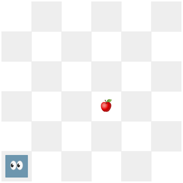
1(a) initial scenario

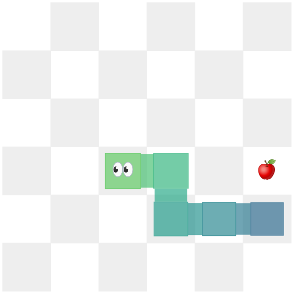
1(b) step - before

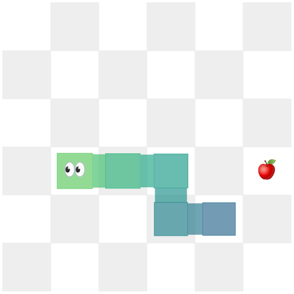
1(c) step - after

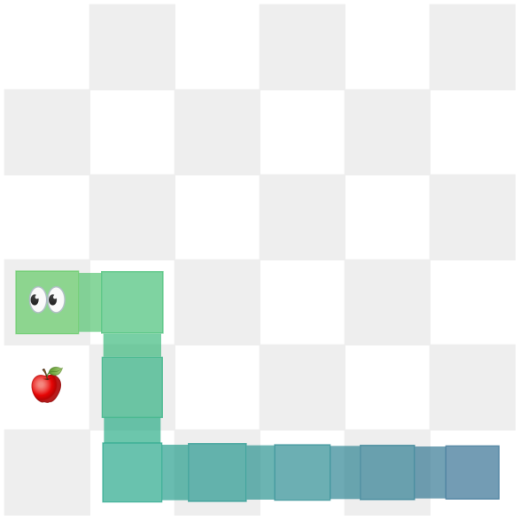
1(d) apple - before

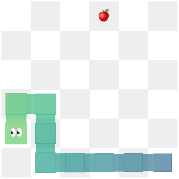
1(e) apple - after

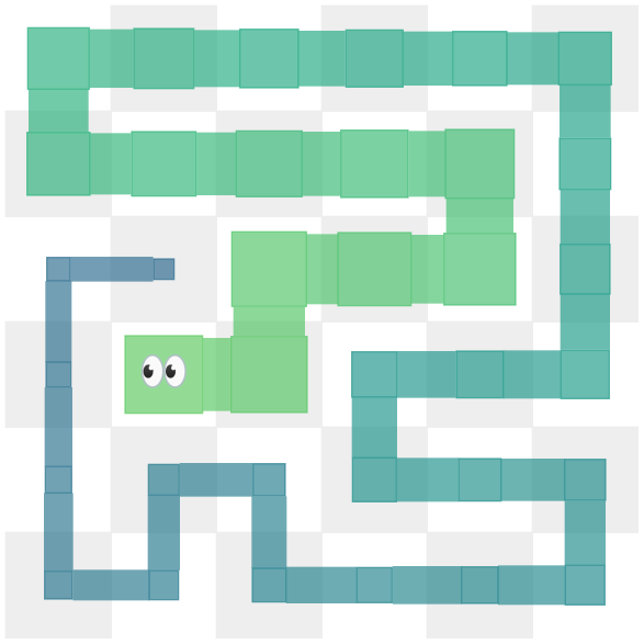
1(f) maximal length

Figure 1: Examples for a snake on a $6\times{}6$ grid generated by our software. The snake head is marked with eyes.

The game snake is a classic arcade game, where the user steers a snake’s head on a grid similar to a grid graph of dimension $n{\times}m$. The snake $\pdftooltip{\includegraphics[height=7.20007pt]{img/snake.eps}}{snakesymbol}{}$ can be interpreted as a list of grid coordinates, for example $\pdftooltip{\includegraphics[height=7.20007pt]{img/snake.eps}}{snakesymbol}{}=[(6,2),(5,2),(4,2),(4,3),(3,3)]$ for Figure 11(b) starting with the tail and ending with the head. Possible movements for the head are left, right, up and down to reach adjacent fields on the grid. The snake body follows the head movement, meaning starting with $\pdftooltip{\includegraphics[height=7.20007pt]{img/snake.eps}}{snakesymbol}{}$ after one step the new snakes $\pdftooltip{\includegraphics[height=7.20007pt]{img/snake.eps}}{snakesymbol}{}^{\prime}$ body elements $\pdftooltip{\includegraphics[height=7.20007pt]{img/snake.eps}}{snakesymbol}^{\prime}{}_{i-1}$ now equal $\pdftooltip{\includegraphics[height=7.20007pt]{img/snake.eps}}{snakesymbol}{}_{i}$ as illustrated in Figures 11(b),11(c).

A snake $\pdftooltip{\includegraphics[height=7.20007pt]{img/snake.eps}}{snakesymbol}{}$ can increase its length by placing the head on a tile occupied by an apple with coordinates $\pdftooltip{\includegraphics[height=7.20007pt]{img/apple.eps}}{applesymbol}{}$, leading for the extended snake $\pdftooltip{\includegraphics[height=7.20007pt]{img/snake.eps}}{snakesymbol}{}^{\prime}$ to occupy the fields $[\pdftooltip{\includegraphics[height=7.20007pt]{img/snake.eps}}{snakesymbol}{}_{1},\dots,\pdftooltip{\includegraphics[height=7.20007pt]{img/snake.eps}}{snakesymbol}{}_{|\pdftooltip{\includegraphics[height=4.20007pt]{img/snake.eps}}{snakesymbolinindexsize}{}|},\pdftooltip{\includegraphics[height=7.20007pt]{img/apple.eps}}{applesymbol}{}]$ as illustrated in Figures 11(d), 11(e). Now the apple is consumed and another apple appears on a random, unoccupied field. The game starts with a snake of length one in the corner of the grid ($\pdftooltip{\includegraphics[height=7.20007pt]{img/snake.eps}}{snakesymbol}=[(1,1)]$) and one apple on a random, unoccupied field as indicated in Figure 11(a). The maximal length of a snake is $n{\cdot}m$, since the snake fills all the fields and no apple can be placed, preventing any future growth of the snake as shown in Figure 11(f). The game terminates if the head lands on a field of the body, leaves the grid, or the snake reached its maximal length. For the latter the game is considered won.

3 Formalizing and Winning snake Optimally with ASP

We introduced the preliminaries and the game snake. We will now move towards defining the game objectives, then presenting strategies and their implementation in ASP.

Goal Specification.

The game itself invokes the implicit goal to maximize the snake length before the game terminates. Our first objective is to guarantee winning the game. This means at every point the snake is able to reach maximal length, independent of apple placement (G1). Second, we aim to minimize the number of snake movements (steps) to finish the game (G2). Third, we aim to minimize the computation time (G3).

3.1 Problem Description for Iterations

One snake game consists of $n{\cdot}m{-}2$ iterations of searching a path from a given snake snake symbol to a given apple apple symbol for given grid dimensions $n{\times}m$. Therefore, we can formalize a problem description for one iteration.

General Snake. Given a path $\pdftooltip{\includegraphics[height=7.20007pt]{img/snake.eps}}{snakesymbol}{}$, a goal vertex $\pdftooltip{\includegraphics[height=7.20007pt]{img/apple.eps}}{applesymbol}{}\not\in\{\pdftooltip{\includegraphics[height=7.20007pt]{img/snake.eps}}{snakesymbol}{}_{1},\cdots,\pdftooltip{\includegraphics[height=7.20007pt]{img/snake.eps}}{snakesymbol}{}_{|\pdftooltip{\includegraphics[height=4.20007pt]{img/snake.eps}}{snakesymbolinindexsize}{}|}\}$ on a grid graph $G(n,m)$, derive a path $\textit{p}{}=[\pdftooltip{\includegraphics[height=7.20007pt]{img/snake.eps}}{snakesymbol}{}_{1},\cdots,\pdftooltip{\includegraphics[height=7.20007pt]{img/snake.eps}}{snakesymbol}{}_{|\pdftooltip{\includegraphics[height=4.20007pt]{img/snake.eps}}{snakesymbolinindexsize}{}|},\cdots,\pdftooltip{\includegraphics[height=7.20007pt]{img/apple.eps}}{applesymbol}{}]$, such that $p_{a}=\pdftooltip{\includegraphics[height=7.20007pt]{img/apple.eps}}{applesymbol}{}$ iff $a=|\textit{p}{}|$ and for every $1{\leq}j{<}k{<}|\textit{p}{}|$ with $\textit{p}{}_{j}=\textit{p}{}_{k}$, then $k-j\geq{}|\pdftooltip{\includegraphics[height=7.20007pt]{img/snake.eps}}{snakesymbol}|$.

General Snake has three key points: the path has to start with snake symbol, the apple symbol vertex appears exactly once at the end and if a vertex repeats, enough steps lie between repetitions for the snake to move out of the way. General Snake covers all possible solutions for one iteration of snake.

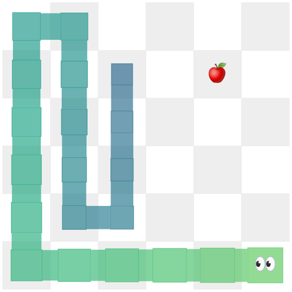
2(a) HC input

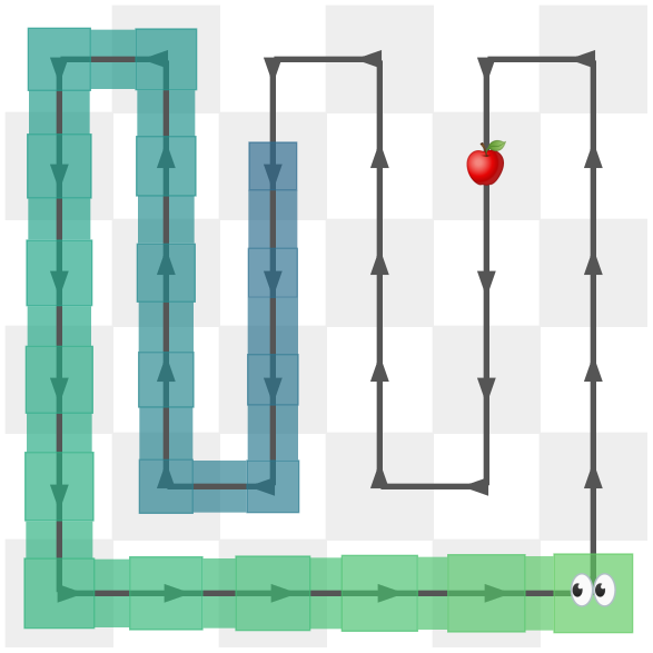
2(b) Generic HC

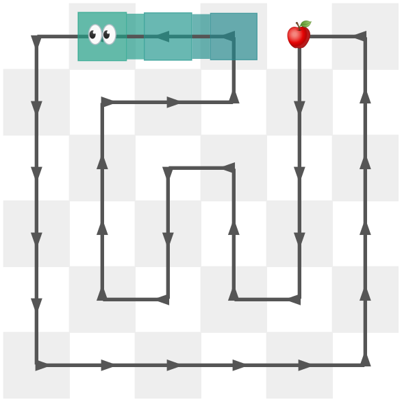
2(c) MHS

Figure 2: Examples for a snake on a $6\times{}6$ grid. Black lines indicate HCs.

While this problem description is sound to solve a single iteration, it does not ensure future iterations to be solvable (compare Figures 11(d), 11(e)). To force a game to be won (G1), each field has to be reachable in every iteration. An effective method to enforce reachability in all future iterations is deriving HCs, since the snake will visit each field of the grid before reaching the field currently occupied by its tail. Hence, we define two problems which include HCs as well, where the second is an extension of the first.

Hamiltonian Snake (HS). Given a path $\pdftooltip{\includegraphics[height=7.20007pt]{img/snake.eps}}{snakesymbol}{}$ for a grid graph $G(n,m)$, derive an HC on $G$ starting with subpath snake symbol.

Minimal Hamiltonian Snake (MHS). Given a path $\pdftooltip{\includegraphics[height=7.20007pt]{img/snake.eps}}{snakesymbol}{}$ and a goal vertex apple symbol with $\pdftooltip{\includegraphics[height=7.20007pt]{img/apple.eps}}{applesymbol}{}\not\in{}\{\pdftooltip{\includegraphics[height=7.20007pt]{img/snake.eps}}{snakesymbol}{}_{1},\cdots,\pdftooltip{\includegraphics[height=7.20007pt]{img/snake.eps}}{snakesymbol}{}_{|\pdftooltip{\includegraphics[height=4.20007pt]{img/snake.eps}}{snakesymbolinindexsize}{}|}\}$ for a grid graph $G(n,m)$, derive an HC on $G$ starting with subpath $\pdftooltip{\includegraphics[height=7.20007pt]{img/snake.eps}}{snakesymbol}{}$ which minimizes $i$ for $\textit{p}_{i}=\pdftooltip{\includegraphics[height=7.20007pt]{img/apple.eps}}{applesymbol}{}$.

An example of the problem and its (minimal) Hamiltonian snake can be seen in Figures 22(a), 22(b). Since HCs can only be derived for grid graphs with even numbers of vertices (Itai et al., 1982), we will handle grids with even number of fields only.

Complexity.

HS asks for a solution of an NP problem, putting in the complexity class of nondeterministic polynomial Function Problems (FNP). MHS asks for a solution of an NP problem for which no other solutions with certain properties exist, putting MHS in the complexity class of FNP with NP oracle calls ($\textsc{FNP}{}^{\textsc{NP}{}}$). We decided to define function problems, since strategies (see next paragraph) require actual paths as output.

3.2 Snake Strategies

To solve a whole snakes game, we will iteratively solve its $n{\cdot}m{-}2$ HS resp. MHS problems (basic setup). Starting in the first iteration with $\pdftooltip{\includegraphics[height=7.20007pt]{img/snake.eps}}{snakesymbol}{}=[(1,1)]$, every iteration has a starting snake snake symbol and random apple coordinates $\pdftooltip{\includegraphics[height=7.20007pt]{img/apple.eps}}{applesymbol}\not\in\{\pdftooltip{\includegraphics[height=7.20007pt]{img/snake.eps}}{snakesymbol}{}_{1},\ldots,\pdftooltip{\includegraphics[height=7.20007pt]{img/snake.eps}}{snakesymbol}{}_{|\pdftooltip{\includegraphics[height=4.20007pt]{img/snake.eps}}{snakesymbolinindexsize}{}|}\}$ as variable input. From the output path $\textit{p}{}=[\pdftooltip{\includegraphics[height=7.20007pt]{img/snake.eps}}{snakesymbol}{}_{1},\ldots{},\pdftooltip{\includegraphics[height=7.20007pt]{img/snake.eps}}{snakesymbol}{}_{|\pdftooltip{\includegraphics[height=4.20007pt]{img/snake.eps}}{snakesymbolinindexsize}{}|},\ldots,\textit{p}{}_{j},\ldots{},\textit{p}{}_{nm}]$ with $\textit{p}{}_{j}=\pdftooltip{\includegraphics[height=7.20007pt]{img/apple.eps}}{applesymbol}{}$ we can derive the snake coordinates $\pdftooltip{\includegraphics[height=7.20007pt]{img/snake.eps}}{snakesymbol}{}^{\prime}$ for the next iteration: $\pdftooltip{\includegraphics[height=7.20007pt]{img/snake.eps}}{snakesymbol}{}^{\prime}=[\textit{p}{}_{j-|\pdftooltip{\includegraphics[height=4.20007pt]{img/snake.eps}}{snakesymbolinindexsize}|},\ldots{},\textit{p}{}_{j}]$.

We will now introduce the naive strategy, which aims to finish the game consistently by solving its HS problems. In the first iteration, the naive strategy derives an HC. This path is followed repeatedly, removing the requirement to generate new HCs altogether. This strategy takes on average $\nicefrac{{(nm-|\pdftooltip{\includegraphics[height=4.20007pt]{img/snake.eps}}{snakesymbolinindexsize}{}|+1)}}{{2}}$ steps per iteration. The first HC can be derived in polynomial time, by replicating column two and three and row three from Figure 22(b) for arbitrary grid sizes. The number of steps per iteration is bound by the number of fields, consequently putting the naive strategy in polynomial time as well.

The naive strategy aims playing safe (G1). To minimize the total number of steps (G2) we introduce the conservative strategy, which allows the HC to change in between iterations. Hence, we follow the basic setup and solve MHS problems. Solving MHS lies in $\textsc{FNP}{}^{\textsc{NP}{}}$, which places the conservative strategy in the same complexity class.

Addressing the computation time (G3) we have to discuss and compare different implementations and design choices, which will be covered throughout this publication.

3.3 Multi-Shot Implementation Approaches

By following the conservative strategy, playing snakes boils down to generating HCs efficiently. ASP is well suited for this task, NP-Problems can be easily expressed. Furthermore, snake can be implemented quite space efficient as well: Algorithm 1 shows the base logic program for the initial iteration, with head/1 and apple/1 as variable input. field/1 defines the nodes of the grid, connected/2 the edges, next/2 represent the path choices and path/1 ensures a closed cycle. Finally, with mark/1 the path segment between head and apple is marked to be minimized in the last line. In latter iterations, a snake body can be enforced by manipulating corresponding next/2 atoms.

Input: grid dimension $\texttt{n}\times{}\texttt{m}$, position of head (head/1) and apple (apple/1)

1

2field((X,Y)) :- X=1..n, Y=1..m.

3 connected((X,Y1),(X,Y2)) :- |Y1-Y2|=1, field((X,Y1)), field((X,Y2)).

4 connected((X1,Y),(X2,Y)) :- |X1-X2|=1, field((X1,Y)), field((X2,Y)).

5

61 { next(XY,XY') : field(XY ), connected(XY,XY') } 1 :- field(XY').

7 1 { next(XY,XY') : field(XY'), connected(XY,XY') } 1 :- field(XY ).

8

9path(XY) :- field(XY), head(XY).

10path(Next) :- path(XY), next(XY,Next).

11 :- field(XY), not path(XY).

12

13mark(XY) :- field(XY), head(XY).

14mark(Next) :- mark(XY), next(XY,Next), not apple(XY).

#minimize{ 1,XY : mark(XY) }.

Algorithm 1 base logic program to solve one iteration of snakes

ASP base Algorithm 1 can be utilized to iteratively solve snake in different ways. A simple approach is to ground and solve the logical program for each iteration and discard it afterwards (one-shot). However, there are several reasons to reuse a logic program. For instance, time intense grounding or minimal changes can be exploited, especially for iterative progressing problems. There are several approaches to reuse a logic program. Main contribution of this work is a compilation and demonstration of different approaches. Therefore, we will now introduce five different clingo implementations to solve snake. Technically, they will mainly differ in the method to manipulate next/2 atoms.

An outline of the wrapper functionality for multi-shot approaches can be seen in Algorithm 2, which implements the conservative strategy. In Lines 1-3 the logic program, snake symbol and step counter are initialized. The initialization (Line 1) for multi-shot approaches includes grounding apple/1 and head/1 as externals:
....#external apple(XY): field(XY).
....#external head(XY) : field(XY).
Without these (external) atoms, the optimization statement can not be formulated. In a loop, apple symbol is picked at random (Line 5) and corresponding external values for the apple position and snake head are set (Lines 6, 7, 9, 10). The main part is represented by he retrieve function (Line 8). Here, the values of snake symbol will be tied to corresponding next/2 atoms from the logic program. Furthermore, the solve process is started and resulting models are managed and converted into paths. The implementation of the retrieve function depends on the approach (see Algorithms 3-8). In Line 11, the new snake position is derived from the path. The for loop stops once snake symbol reached maximal length or no path could be derived.

Input: grid dimension $n\times{}m$

Output: number of total steps

$\Pi\leftarrow\textit{init}(n,m)$

  // ground Algorithm 1; apple & head as external

$\pdftooltip{\includegraphics[height=7.20007pt]{img/snake.eps}}{snakesymbol}{}\leftarrow[(1,1)]$

  // snake symbol starts at position (1,1) with |snake symbol|=1

$\textit{steps}\leftarrow 0$

  // step counter

1 do ​:

       $\pdftooltip{\includegraphics[height=7.20007pt]{img/apple.eps}}{applesymbol}{}\leftarrow\textit{generate\_apple}((n,m),\pdftooltip{\includegraphics[height=7.20007pt]{img/snake.eps}}{snakesymbol}{})$

        // place on random, non-snake symbol field

2      

      $\Pi\leftarrow\textit{set\_external}(\Pi,\texttt{apple(}\pdftooltip{\includegraphics[height=7.20007pt]{img/apple.eps}}{applesymbol}{}\texttt{)},\textit{True})$

        // set external atoms

3       $\Pi\leftarrow\textit{set\_external}(\Pi,\texttt{head(}\pdftooltip{\includegraphics[height=7.20007pt]{img/snake.eps}}{snakesymbol}{}_{|\pdftooltip{\includegraphics[height=4.20007pt]{img/snake.eps}}{snakesymbolinindexsize}{}|}\texttt{)},\textit{True})$

       $\Pi,\textit{path}\leftarrow\textit{\text@underline{retrieve}}(\Pi,\pdftooltip{\includegraphics[height=7.20007pt]{img/snake.eps}}{snakesymbol}{})$

        // enforce snake symbol onto next/2, generate path

       $\Pi\leftarrow\textit{set\_external}(\Pi,\texttt{apple(}\pdftooltip{\includegraphics[height=7.20007pt]{img/apple.eps}}{applesymbol}{}\texttt{)},\textit{False})$

        // undo external atoms

4       $\Pi\leftarrow\textit{set\_external}(\Pi,\texttt{head(}\pdftooltip{\includegraphics[height=7.20007pt]{img/snake.eps}}{snakesymbol}{}_{|\pdftooltip{\includegraphics[height=4.20007pt]{img/snake.eps}}{snakesymbolinindexsize}{}|}\texttt{)},\textit{False})$

       $\pdftooltip{\includegraphics[height=7.20007pt]{img/snake.eps}}{snakesymbol}{},s\leftarrow\textit{follow\_path}(\pdftooltip{\includegraphics[height=7.20007pt]{img/snake.eps}}{snakesymbol}{},\textit{path},\pdftooltip{\includegraphics[height=7.20007pt]{img/apple.eps}}{applesymbol}{})$

        // snake symbol follows ${path}$ until apple symbol, $s$ steps

5      

      $\textit{steps}\leftarrow\textit{steps}+\textit{s}$

        // update step count

6      

7while $|\pdftooltip{\includegraphics[height=7.20007pt]{img/snake.eps}}{snakesymbol}{}|<n\cdot{}m$ and not $path=\{\}$

8return steps

Algorithm 2 Main Algorithm for iteratively computing snake paths

One-Shot.

one-shot can be understood as the default approach for logic programs. Here, the current position of the snake and the apple are introduced as facts, resulting in permanently fixing the current values. Each iteration requires grounding and solving a new logic program from scratch. While one-shot sounds rather wasteful (especially in an iterative setting), it comes with clear advantages as well: There is no need to consider mechanics of extending or manipulating logic programs, thus creating a simple, stable, straight forward and easy to debug solution. Therefore one-shot is well suited for fast development projects with easy code maintenance or noncritical execution times.

Implementing one-shot uses a similar outline as Algorithm 2, with small changes. Line 1 would be moved into the loop before the apple placement. Instead of setting externals (Lines 6, 7, 9, 10), facts are added to the logic program before solving:

$\Pi\leftarrow\Pi{}\cup{}\textit{ground}(\{\texttt{apple(}\pdftooltip{\includegraphics[height=7.20007pt]{img/apple.eps}}{applesymbol}{}\texttt{).}\;\texttt{head(}\pdftooltip{\includegraphics[height=7.20007pt]{img/snake.eps}}{snakesymbol}{}_{|\pdftooltip{\includegraphics[height=4.20007pt]{img/snake.eps}}{snakesymbolinindexsize}{}|}\texttt{).}\})$.

The retrieve function for one-shot is outlined in Algorithm 3. The function translates snake symbol into equivalent next atom facts to be added to $\Pi{}$. The program is subsequently solved and the path derived from the model returned. To fit the interface of the multi-shot algorithm, the program $\Pi{}$ is returned as well.

Input: program $\Pi$, snake position list snake symbol

Output: program $\Pi$, path

1 for $i=1\,..\,|\pdftooltip{\includegraphics[height=7.20007pt]{img/snake.eps}}{snakesymbol}{}|{-}1$ :

       $\Pi\leftarrow\Pi\cup\textit{ground}(\{\texttt{next(}\pdftooltip{\includegraphics[height=7.20007pt]{img/snake.eps}}{snakesymbol}{}_{i}\texttt{,}\pdftooltip{\includegraphics[height=7.20007pt]{img/snake.eps}}{snakesymbol}{}_{i{+}1}\texttt{).}\}$)

        // transfer snake symbol values to next/2

2      

$\textit{model}\leftarrow\textit{solve}(\Pi)$

  // generate model

$\textnormal{{return}}\;\Pi,\textit{extract\_path}(\textit{model})$

  // extract path out of model

Algorithm 3 retrieve for one-shot

Ad Hoc.

As for multi-shot implementations, adding and removing rules (Gebser et al., 2019b ; Gebser et al., 2015) will be called the ad hoc variant. Adding rules is comparatively easy, as a program is essentially a set of rules. To disable or remove rules, we utilize external atoms, since their truth values are assigned outside of the logic program. Basically, an external atom is introduced as guard to a temporary rule. Once the external guard is released, the connected rules are released as well. Released externals can not be reused.

We will explain the mechanics through the implementation of the retrieve function from Algorithm 4, fitting into Algorithm 2. In our case an atom of step/1 is declared to be external (Line 1). Now constraints enforcing the current snake symbol positions onto next/2 are added with the external as guard (Line 3). The external is set to True (Line 4) and the program solved. To remove the current restrictions on $\Pi{}$, the external is released afterwards (Line 6) and $\Pi{}$ is suited to be used in another iteration.

In current literature, usually ad hoc is utilized, since it allows adding of previously unspecified rules and atoms. This comes in handy, especially for logic programs with rising horizons. Therefore ad hoc (along with one-shot) is the most flexible of all approaches. On the downside, expanding a ground logic program may require a deeper understanding of its underlying dependencies, as existing rules need to be compliant with the added rules. Reducing the number of temporary rules (to streamline the solving process) poses another challenge, since its realization usually adds complexity to maintain the code.

1

$\Pi\leftarrow\Pi\cup\textit{ground}(\{\texttt{\#external step(}|\pdftooltip{\includegraphics[height=7.20007pt]{img/snake.eps}}{snakesymbol}{}|{\texttt{).}}\})$

  // introducing the guard

2 for $i=1\,..\,|\pdftooltip{\includegraphics[height=7.20007pt]{img/snake.eps}}{snakesymbol}{}|{-}1$ :

       $\Pi\leftarrow\Pi\cup\textit{ground}(\{\texttt{:- }\;\texttt{step(}|\pdftooltip{\includegraphics[height=7.20007pt]{img/snake.eps}}{snakesymbol}{}|\texttt{),}\texttt{ {\color[rgb]{0.328125,0.3828125,0.44921875}not} next(}\pdftooltip{\includegraphics[height=7.20007pt]{img/snake.eps}}{snakesymbol}{}_{i}\texttt{,}\pdftooltip{\includegraphics[height=7.20007pt]{img/snake.eps}}{snakesymbol}{}_{i{+}1}\texttt{).}\}$)

        // adding rules

3      

$\Pi\leftarrow\textit{set\_external}(\Pi,\texttt{step(}|\pdftooltip{\includegraphics[height=7.20007pt]{img/snake.eps}}{snakesymbol}{}|\texttt{)},\textit{True})$

  // activating guard

4 $\textit{model}\leftarrow\textit{solve}(\Pi)$

$\Pi\leftarrow\textit{release\_external}(\Pi,\texttt{step(}|\pdftooltip{\includegraphics[height=7.20007pt]{img/snake.eps}}{snakesymbol}{}|\texttt{)})$

  // removing guard and its rules

$\Pi\leftarrow\textit{cleanup}(\Pi{})$

  // cleanup after release

$\textnormal{{return}}\;\Pi,\textit{extract\_path}(\textit{model})$

  // generate path out of model

Algorithm 4 retrieve for ad hoc;   Input: $\Pi$, snake symbol;   Output: $\Pi$, path

Preground.

In a restricted setting, adding and removing rules might not be a required feature and would result in unnecessary computational overhead. Pregrounding all required temporary rules might improve computation times, reduce complexity of the code and introduces a neat interface between the wrapper program and the logic program. Each temporary rule acquires at least one external predicate in the body to be switched on and off again. Pregrounding does not include the option to add rules on the fly since all possible changes are introduced once in the beginning. Additionally, a vast amount of inactive rules might slow down the program as well. However, preground might perform well on compact programs with lots of iterations, since in comparison to ad hoc no overhead is generated.

Algorithm 2 can be extended for preground by adding the following rules to the initial grounding in Line 1:
#external prenext(X,Y) : connected(X,Y).
:- prenext(X,Y), not next(X,Y), connected(X,Y).
By setting the external prenext/2 to True, we can enforce the corresponding next/2 atom to be True as well. Algorithm 5 indicates the functionality of the retrieve function, which boils down to translating the snake into corresponding prenext/2 atoms and temporary activating them before solving.

1

2for $i=1..|\pdftooltip{\includegraphics[height=7.20007pt]{img/snake.eps}}{snakesymbol}{}|-1$ :

       $\Pi\leftarrow\textit{set\_external}(\Pi,\texttt{prenext(}\pdftooltip{\includegraphics[height=7.20007pt]{img/snake.eps}}{snakesymbol}{}_{i}\texttt{,}\pdftooltip{\includegraphics[height=7.20007pt]{img/snake.eps}}{snakesymbol}{}_{i{+}1}\texttt{)},\textit{True})$

        // enforce snake symbol positions

3      

4$\textit{model}\leftarrow\textit{solve}(\Pi)$

5 for $i=1..|\pdftooltip{\includegraphics[height=7.20007pt]{img/snake.eps}}{snakesymbol}{}|-1$ :

       $\Pi\leftarrow\textit{set\_external}(\Pi,\texttt{prenext(}\pdftooltip{\includegraphics[height=7.20007pt]{img/snake.eps}}{snakesymbol}{}_{i}\texttt{,}\pdftooltip{\includegraphics[height=7.20007pt]{img/snake.eps}}{snakesymbol}{}_{i{+}1}\texttt{)},\textit{False})$

        // deactivate

6      

7$\textnormal{{return}}\;\Pi,\textit{extract\_path}(\textit{model})$

Algorithm 5 retrieve for preground;   Input: $\Pi$, snake symbol;   Output: $\Pi$, path

Assume.

Instead of handling externals and altering the logic program every time, we can also fix truth values for non-external atoms via assumptions. This option is limited to truth values of atoms, therefore in many cases the introduction of auxiliary rules and atoms is advised, comparable to preground. Assumption atoms do not require to be declared as such and they are provided as a list of atom/truth value assignments to the solve call. In comparison to externals, assumptions are not persistent and have to be formulated for every solve call, which may lead to a less organized setup in comparison to preground. The naming convention should also be considered: names of externals are usually picked for easy access in the wrapper program, whereas assumption require to operate on predefined atom names. Handling atoms with complex terms in clingo can become convoluted quite fast, decreasing the readability of the code. assume and preground compare in functionality, with preground contributing a simpler interface and assume being more flexible.

The retrieve function for the assume approach is shown in Algorithm 6. In clingo assumptions are provided as an attribute to the solve call. Enforcing the snake symbol position via assumptions does not require any alterations of the logic program.

$\textit{assume}\leftarrow[\,]$

  // start with empty list of assumptions

1 for $i=1..|\pdftooltip{\includegraphics[height=7.20007pt]{img/snake.eps}}{snakesymbol}{}|-1$ :

       $\textit{assume.append}((\texttt{next(}\pdftooltip{\includegraphics[height=7.20007pt]{img/snake.eps}}{snakesymbol}{}_{i}\texttt{,}\pdftooltip{\includegraphics[height=7.20007pt]{img/snake.eps}}{snakesymbol}{}_{i{+}1}\texttt{)},\textit{True}))$

        // add atom/value tuple

2      

3$\textit{model}\leftarrow\textit{solve}(\Pi,\textit{assumption}=\textit{{assume})}$

4$\textnormal{{return}}\;\Pi,\textit{extract\_path}(\textit{model})$

Algorithm 6 retrieve for assume;   Input: $\Pi$, snake symbol;   Output: $\Pi$, path

Nogood.

Next to assignments of truth values to (external) atoms, clingo also offers mechanics to influence the search progress. During the search, proven sub-results are stored in form of (negated) conjunctions of literals, which are called clauses and nogoods(Weinzierl, 2017). Adding custom nogoods to an ongoing search can be utilized as multi-shot approach. Comparable to assumptions, we are able to assign truth values to not only atoms but clauses during a solve call. The nogood approach therefore can handle rules similar to preground without prior definition, since truth values can be assigned to arbitrary conjunctions of literals. In clingo nogoods require sophisticated knowledge to access: either via a customized propagator or via accessing a model from the solve call. We implemented the latter, which causes the issue of adding constraints after obtaining the initial model. Like this, the first model does not respect the snake placement. This can result in an unobtainable short path, which renders the subsequent optimization futile. However, the system can be steered to generate a predefined model using heuristics as described in the next paragraph.

To manipulate nogoods, a function to process obtained models needs to be assigned in the solve call (here: my_func). The retrieve function boils down to assigning a function for model handling as shown in Algorithm 7.

1 $model\leftarrow{}solve(\Pi,\text{on\_model}=\textit{my\_func})$

$\textnormal{{return}}\;\Pi,\textit{extract\_path}(\textit{model})$

Algorithm 7 retrieve for nogood;   Input: $\Pi$, snake symbol;   Output: $\Pi$, path

The function my_func has access to the model object during the solve call. It is its only argument. Additional objects can be provided via object oriented programming (Gebser et al., 2015). A partial implementation of my_func can be seen in Algorithm 8. At first, the function checks if the current model is the first obtained model and compliant with our not yet enforced restrictions. In our implementation, this model is marked with a special atom (dummy). If this is the case, a clause is added to enforce the current snake placement.

Input: model $model$

1 $\cdots{}$

2 if $\texttt{\text{dummy}}\in\textit{model}$  :

3       for $i=1..|\pdftooltip{\includegraphics[height=7.20007pt]{img/snake.eps}}{snakesymbol}{}|-1$ :

4             $\textit{model.context.add\_clause}(\texttt{next(}\pdftooltip{\includegraphics[height=7.20007pt]{img/snake.eps}}{snakesymbol}{}_{i}\texttt{,}\pdftooltip{\includegraphics[height=7.20007pt]{img/snake.eps}}{snakesymbol}{}_{i{+}1}\texttt{)},\textit{True})$

$\cdots{}$

Algorithm 8 my_func - code snipped to add snake symbol as search restriction

To summarize: The nogood approach combines the possible expressivity of preground without the baggage of inactive rules with the flexibility of assumptions. However, access to nogoods requires sophisticated knowledge of the clingo API. If the nogoods are set via the model object, mechanics to enforce a predefined first model might be necessary.

Initial Model via Heuristics.

For the introduced strategies, we can generate one HC from the previous iteration or a generic HC for the first iteration (compare Figure 22(a)). Therefore, we can jump-start the current solve process, guaranteeing at least one model for the optimization in the conservative strategy. We can utilize heuristics (Gebser et al., 2019a ) to inject this dummy model within the logic program in clingo:
……{dummy}.
……#heuristic dummy. [ 99, true]
……#external heur(X,Y) : connected(X,Y).
……:- dummy, heur(X,Y), not next(X,Y).
For this, an independent dummy atom is introduced and marked with a high preference to be set to True. Additional external atoms (i.e. heur/2) can be preset to influence the actual effect of the dummy atom to the models where it is contained. We are now able to set a dummy model, which benefits computation times and is required to implement the nogood approach via model object.

4 Experimental Evaluation

Setup.

To compare performance of the different approaches, we implemented all five approaches of the conservative strategy and let them solve 100 snake games for different square grid sizes ($n=m,n\in\{6,8,10,12,14,16\}$). The experiments run on a MacBook Pro (2017, 16 GB RAM, Intel Core i7, 2.8 GHz), with clingo v. 5.4.0 and python v. 3.7.4. For each run, each of the $n\cdot{}m{-}2$ iterations has a 60 seconds timeout for the solve call. Image generation via clingraph (Hahn et al., 2022) is disabled.

We utilize a symmetry breaking method to mirror the grid, such that the head always lies in the first quadrant of the grid. We used ASP-Chef (Alviano et al., 2023) for prototyping of the logic program. Our implementation and logfiles are available online.

	$n\times{}m$	$6\times{}6$	$8\times{}8$	$10\times{}10$	$12\times{}12$	$14\times{}14$	$16\times{}16$
	one-shot	213	576	1235	2441	5519	10157
	ad hoc	208	572	1226	2411	4582	7445
(a)	preground	216	563	1236	2374	4540	7482
	assume	210	563	1234	2396	4508	7540
	nogood	212	559	1240	2428	4580	7523
	one-shot	0.159	2.28	71.83	621	2216	4359
	ad hoc	0.066	3.42	90.07	674	1966	3869
(b)	preground	0.060	3.32	94.71	620	1978	3870
	assume	0.059	4.78	97.48	628	1944	3853
	nogood	0.061	3.16	94.70	702	1951	3877

Table 1: (a) Average number of total steps per run. Outliers are underlined.
(b) Average total time per game in seconds, timeout $60s$, best value bold.

Evaluation.

We expect snake to be feasible to a certain extend (E1). Furthermore, we expect multi-shot and one-shot to differ performance wise (E2) and we expect multi-shot to outperform one-shot due to the grounding bottleneck (E3). As educated guess, we expect ad hoc to outperform preground based on unused externals (E4). Due to implementation details, we expect assume to terminate slightly faster than nogood (E5).

According to our three objectives, we are interested in three features: the win/loose ratio (G1), the number of total steps (G2) and the total time (G3). Since our strategy uses the previous HC as starting model, there is a $100\%$ win ratio and G1 is fully met. For G2, we compare the total number of steps, which are listed in Table 1(a). For most grid sizes the numbers do not vary significantly. This is not surprising, since they implement the same algorithm. However one-shot falls behind for larger grid sizes ($n\geq{}14$, E2).

As for the total time (G3, Table 1(b)), the multi-shot approaches do not differ significantly except for one-shot (E2). For grid $6{\times}6$, the grounding impacts the total time negatively, placing one-shot last (E3). This changes for grid sizes $8{\times}8$ and $10{\times}10$, where one-shot consistently leads in total time. For $12{\times}12$ time consumption is on par and for larger grids ($14{\times}14$, $16{\times}16$) one-shot has the highest total time.

The data hint a disadvantage for one-shot for larger grids, therefore we will analyze the step count per iteration as seen in Figure 3. For each grid size, the average number of steps to reach the apple is plotted against the iteration number, which equals the current length of the snake. The expected step count for the naive strategy is hinted as gray dotted line. For smaller grids (${<}12{\times}12$) all implementations perform on par and the curves show roughly the same pattern. For grid $10{\times}10$ the curve pattern changes. This can be explained with the timeout ratio (colored dashed line), meaning all approaches would have required more time to finish the optimization in the first iterations. The timeout was triggered for grid $8{\times}8$ as well, but seemed to mainly affect the last step of confirming the optimum, while for $10{\times}10$ the timeout took place during the active optimization phase (E1). For grid $12{\times}12$ the curves for the different approaches do not differ much. However, for grids $14{\times}14$ and $16{\times}16$ the curve for one-shot differs significantly from the multi-shot approaches: During the first iteration, all multi-shot approaches face the same timeout rate and impact as one-shot. However, their performance improves substantially faster in the following iterations. We assume the multi-shot advantage is based on utilizing past search progress in form of learned nogoods and seems to increase for larger grid sizes.

The different multi-shot approaches operate on similar levels. assume performed best in terms of computation times. However, the differences are minor and vary for different setups. As educated guess, we would expect an advantage of ad hoc over preground for high amounts of temporary rules. Our preground implementation introduces a comparatively small number of temporary rules and the data do not support a disadvantage of pregroundfor this implementation (E4). Also, we expect assume to outperform nogood, since the handling of the nogoods counts towards the solving time. This advantage is probably too minor to manifest in the data (E5).

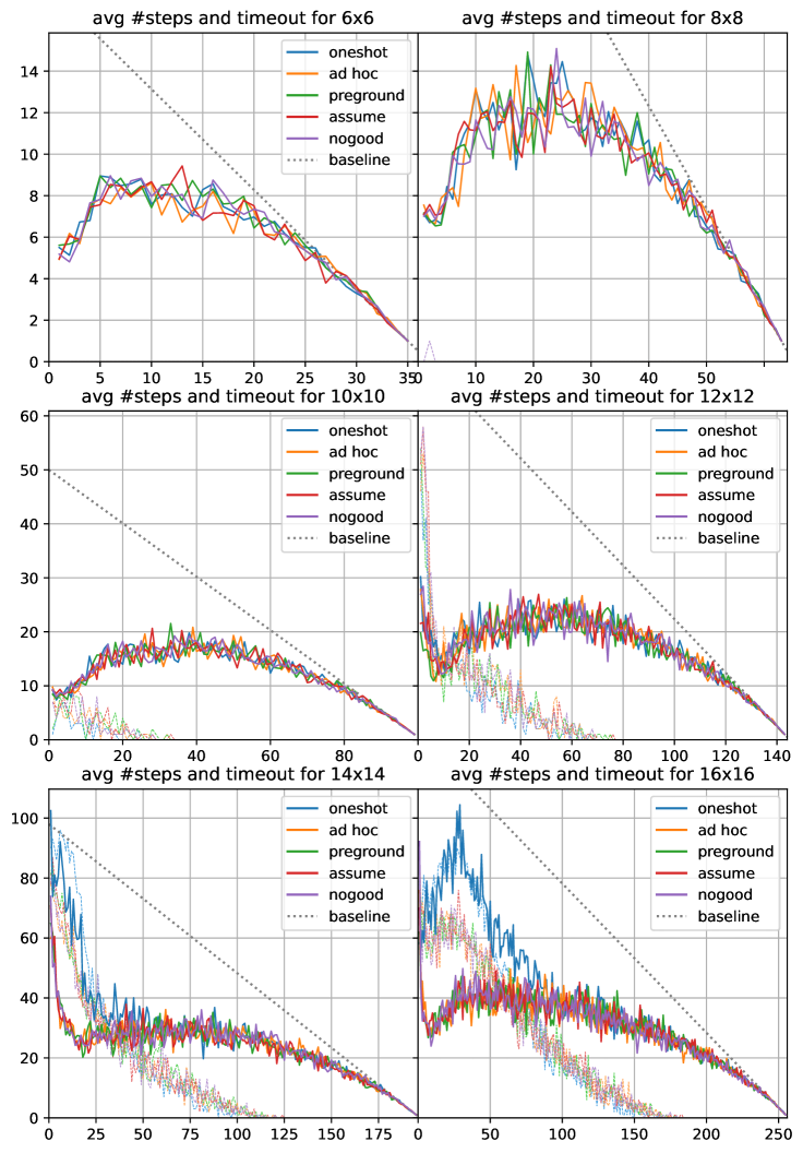
Figure 3: Average number of steps (solid lines) and timeout rate in percent (dashed lines) per iteration for different grid sizes for timeout 60s. Dotted gray line is the expected step count for the naive strategy (baseline).

Summary.

All approaches guarantee winning snakes. one-shot dominated the comparison, until resources were limited by the timeout. The other approaches struggled with the timeout as well, but could utilize the previous solving history, leading to a reduction of timeouts through the iterations. The multi-shot approaches performed on similar levels, individual rankings were not consistent throughout different setups.

Related Work

HCs for grid graphs are well studied (Itai et al., 1982). ASP was utilized to find HCs in general graphs (Hirate et al., 2023; Liu and Truszczynski, 2019). Several implementations for AI approaches on playing snake are available. A variety of search algorithms is used to play snake, varying from basic strategies such as A* and HCs (Appaji, 2020) to more sophisticated approaches (Yeh et al., 2016; Wei et al., 2018). To our knowledge no further snake implementation in logic programming has been proposed. However, multi-shot ASP has been used to solve iterative games such as Towers of Hanoi (Gebser et al., 2019b ) and Ricochet Robots (Gebser et al., 2015). Several (iterative) games are already implemented in ASP, such as Rush Hour (Cian et al., 2022), Sokoban (Gebser et al., 2008) and Icosoku (Rizzo and Dovier, 2022).

Other solvers such as DLV2 support multi-shot as well (Calimeri et al., 2022).

5 Conclusion and Future Work

This paper aims to compile different ASP multi-shot approaches on an compact and hands-on showcase. While one-shot is straightforward to implement, applications with limited resources (such as timeouts) may substantially benefit from multi-shot implementations, as demonstrated in our evaluation. For our example, the grounding bottleneck was not an issue due to a minimalistic implementation. one-shot outperformed the multi-shot approaches as long as the timeout was not met. For harder problems, the timeout had a huge impact on the performance. The multi-shot approaches could utilize the search progress from previous solving attempts, reducing the impact of the timeout in the following iterations and therefore outperforming one-shot. The different multi-shot approaches possess varying characteristics, therefore the optimal choice depends on the application and the setup. The approaches ad hoc and assume have indicated stable performance and are comparatively easy to implement.

Future work might entail another showcase application to demonstrate performance differences between the different multi-shot approaches. In addition, while the definition of MHS is sound, a different problem description may lead to even shorter paths while still guaranteeing winning the game. An example scenario can be seen in Figure 22(c), where shorter paths to enforcing a win can be derived. For this more sophisticated problem only the snake end positioning has to be able to form an HC. However, this new problem, resulting strategies, extended implementations and additional evaluation go beyond the scope of this paper. Also, the introduced strategies rely on a continuous setting, meaning our strategies can not be started from an arbitrary snake placement as seen in Figure 11(d). Strategies starting with random snake placements may be covered in the future.

Acknowledgments

The authors are stated in alphabetic order. This work was supported by BMBF in project 01IS20056_NAVAS and in BMBF grant ITEA-01IS21084 (InnoSale), DFG grant 389792660 (TRR 248), and in DAAD grant 57616814 (SECAI).

References

- Adrian et al., (2018) Adrian, W. T., Alviano, M., Calimeri, F., Cuteri, B., Dodaro, C., Faber, W., Fuscà, D., Leone, N., Manna, M., Perri, S., and others 2018. The ASP system DLV: advancements and applications. KI-Künstliche Intelligenz, 32, 177–179.
- Alviano et al., (2023) Alviano, M., Cirimele, D., and Reiners, L. A. R. Introducing ASP recipes and ASP chef. In Proc. of LPNMR’23 2023.
- Alviano et al., (2013) Alviano, M., Dodaro, C., Faber, W., Leone, N., and Ricca, F. WASP: A native ASP solver based on constraint learning. In Proc. of LPNMR’13 2013, pp. 54–66. Springer.
- Appaji, (2020) Appaji, N. S. D. 2020. Comparison of searching algorithms in AI against human agent in the snake game. Bachelor Thesis, Blekinge Institute of Technology,.
- Besin et al., (2023) Besin, V., Hecher, M., and Woltran, S. On the structural complexity of grounding - tackling the ASP grounding bottleneck via epistemic programs and treewidth. In Proc. of ECAI’23 2023, volume 372 of FAIA, pp. 247–254. IOS Press.
- Brewka et al., (2011) Brewka, G., Eiter, T., and Truszczyński, M. 2011. Answer set programming at a glance. Communications of the ACM, 54, 12, 92–103.
- Calimeri et al., (2019) Calimeri, F., Faber, W., Gebser, M., Ianni, G., Kaminski, R., Krennwallner, T., Leone, N., Maratea, M., Ricca, F., and Schaub, T. 2019. ASP-core-2 input language format. CoRR, abs/1911.04326.
- Calimeri et al., (2022) Calimeri, F., Ianni, G., Pacenza, F., Perri, S., and Zangari, J. ASP-based multi-shot reasoning via DLV2 with incremental grounding. In Proc. of PPDP’22 2022.
- Cian et al., (2022) Cian, L., Dreossi, T., Dovier, A., and others. Modeling and solving the rush hour puzzle. In CEUR Workshop Proceedings 2022, volume 3204, pp. 294–306.
- Comploi-Taupe et al., (2023) Comploi-Taupe, R., Friedrich, G., Schekotihin, K., and Weinzierl, A. 2023. Domain-specific heuristics in answer set programming: A declarative non-monotonic approach. Journal of Artificial Intelligence Research, 76.
- De Biasi and Ophelders, (2016) De Biasi, M. and Ophelders, T. The complexity of snake. In Proc. of FUN’16 2016.
- Gaggl et al., (2015) Gaggl, S. A., Manthey, N., Ronca, A., Wallner, J. P., and Woltran, S. 2015. Improved answer-set programming encodings for abstract argumentation. TPLP, 15, 4-5, 434–448.
- (13) Gebser, M., Kaminski, R., Kaufmann, B., Lindauer, M., Ostrowski, M., Romero, J., Schaub, T., Thiele, S., and Wanko, P. 2019a. Potassco User Guide, version 2.2.0 edition.
- Gebser et al., (2008) Gebser, M., Kaminski, R., Kaufmann, B., Ostrowski, M., Schaub, T., and Thiele, S. Engineering an incremental asp solver. In Logic Programming 2008, pp. 190–205. Springer.
- (15) Gebser, M., Kaminski, R., Kaufmann, B., and Schaub, T. 2019b. Multi-shot ASP solving with clingo. TPLP, 19b, 1, 27–82.
- Gebser et al., (2015) Gebser, M., Kaminski, R., Obermeier, P., and Schaub, T. 2015. Ricochet Robots Reloaded: A Case-Study in Multi-shot ASP Solving, pp. 17–32. Springer.
- Gebser et al., (2011) Gebser, M., Kaufmann, B., Kaminski, R., Ostrowski, M., Schaub, T., and Schneider, M. 2011. Potassco: The potsdam answer set solving collection. AI Communic., 24, 107–124.
- Gelfond and Lifschitz, (1988) Gelfond, M. and Lifschitz, V. The stable model semantics for logic programming. In ICLP/SLP 1988, volume 88, pp. 1070–1080. Cambridge, MA.
- Hahn et al., (2022) Hahn, S., Sabuncu, O., Schaub, T., and Stolzmann, T. Clingraph: ASP-based visualization. In Proc. of LPNMR’22 2022, volume 13416 of LNCS, pp. 401–414. Springer.
- Hirate et al., (2023) Hirate, T., Banbara, M., Inoue, K., Lu, X.-N., Nabeshima, H., Schaub, T., Soh, T., and Tamura, N. Hamiltonian cycle reconfiguration with answer set programming. In Proc. of JELIA’23 2023, 262–277. Springer.
- Itai et al., (1982) Itai, A., Papadimitriou, C. H., and Szwarcfiter, J. L. 1982. Hamilton paths in grid graphs. SIAM Journal on Computing, 11, 4, 676–686.
- Liu and Truszczynski, (2019) Liu, L. and Truszczynski, M. Encoding selection for solving hamiltonian cycle problems with ASP. In Proc. of ICLP’19 2019, volume 306 of EPTCS, pp. 302–308.
- Rajaratnam et al., (2023) Rajaratnam, D., Schaub, T., Wanko, P., Chen, K., Liu, S., and Son, T. C. 2023. Solving an industrial-scale warehouse delivery problem with answer set programming modulo difference constraints. Algorithms, 16, 4, 216.
- Rizzo and Dovier, (2022) Rizzo, N. and Dovier, A. 2022. 3cosoku and its declarative modeling. Journal of Logic and Computation, 32, 2, 307–330.
- Takeuchi et al., (2023) Takeuchi, R., Banbara, M., Tamura, N., and Schaub, T. Solving vehicle equipment specification problems with answer set programming. In Proc. of PADL 2023, pp. 232–249. Springer.
- Thielscher, (2009) Thielscher, M. Answer set programming for single-player games in general game playing. In Logic Programming 2009, pp. 327–341. Springer.
- Wei et al., (2018) Wei, Z., Wang, D., Zhang, M., Tan, A.-H., Miao, C., and Zhou, Y. Autonomous agents in snake game via deep reinforcement learning. In Proc. of ICA’18 2018. IEEE.
- Weinzierl, (2017) Weinzierl, A. Blending lazy-grounding and cdnl search for answer-set solving. In Proc. of LPNMR’17 2017, pp. 191–204. Springer.
- Yeh et al., (2016) Yeh, J.-F., Su, P.-H., Huang, S.-H., and Chiang, T.-C. Snake game AI: Movement rating functions and evolutionary algorithm-based optimization. In Proc. of TAAI’16 2016. IEEE.