Impact of Comprehensive Data Preprocessing on Predictive Modelling of COVID-19 Mortality

Abstract

Accurate predictive models are crucial for analysing COVID-19 mortality trends. This study evaluates the impact of a custom data preprocessing pipeline on ten machine learning models predicting COVID-19 mortality using data from Our World in Data (OWID). Our pipeline differs from a standard preprocessing pipeline through four key steps. Firstly, it transforms weekly reported totals into daily updates, correcting reporting biases and providing more accurate estimates. Secondly, it uses localised outlier detection and processing to preserve data variance and enhance accuracy. Thirdly, it utilises computational dependencies among columns to ensure data consistency. Finally, it incorporates an iterative feature selection process to optimise the feature set and improve model performance. Results show a significant improvement with the custom pipeline: the MLP Regressor achieved a test RMSE of 66.556 and a test R² of 0.991, surpassing the DecisionTree Regressor from the standard pipeline, which had a test RMSE of 222.858 and a test R² of 0.817. These findings highlight the importance of tailored preprocessing techniques in enhancing predictive modelling accuracy for COVID-19 mortality. Although specific to this study, these methodologies offer valuable insights into diverse datasets and domains, improving predictive performance across various contexts.

I Introduction

The COVID-19 pandemic has profoundly disrupted global health systems and daily life, presenting unprecedented challenges in disease management and resource allocation. Since the emergence of Severe Acute Respiratory Syndrome Coronavirus 2 (SARS-CoV-2) in December 2019, the pandemic has resulted in extensive morbidity and mortality worldwide. In India, where the first cases were reported in January 2020 [1], the impact has been particularly severe, with over 45 million confirmed cases and more than 530,000 deaths as of July 2024 [2]. The pandemic disproportionately affected older adults and individuals with pre-existing health conditions such as hypertension, diabetes, and cardiovascular disease [3, 4].

As the pandemic progressed, the need for accurate predictive models to guide healthcare planning and resource allocation became increasingly critical [5, 6, 7, 8, 9, 10, 11]. The foundation of these models depends heavily on the quality of data and the preprocessing steps applied, both of which are crucial for ensuring the reliability of predictions [12, 13, 14, 15]. Robust preprocessing transforms raw data into meaningful features through techniques such as dropping irrelevant columns [16, 17, 18, 19, 20], creating new features [21], and renaming columns [22]. Imputing missing values using zero, mean, or median values, along with interpolation and extrapolation methods [23, 24, 25, 26, 27, 28, 29, 17, 30, 31] ensures that gaps in the data do not compromise the model accuracy. Outlier processing—whether through dropping, trimming, transforming, or winsorizing [32, 33, 34, 26], preserves data integrity by addressing anomalies. Feature selection, using methods such as correlation [35], principal component analysis (PCA) [31], random feature exploration [17], ranking features through univariate and multivariate filter methods, and wrapper methods [20, 36] optimizes model performance by reducing multicollinearity and eliminating redundant features [37]. These steps are essential for enhancing the reliability and accuracy of predictive models [38, 39].

Despite significant advancements in predictive modelling, many current approaches prioritize model development over thorough data preprocessing. This oversight often results in a superficial understanding of the data, neglecting its inherent patterns, relationships, and dependencies, crucial for developing robust models. For instance, failing to account for weekly reporting patterns can distort model training and degrade performance. Ignoring computational dependencies between columns can introduce inconsistencies, undermining the integrity of the entire modelling process. Moreover, using global outlier detection methods with fixed thresholds, such as z-scores, fails to accommodate the local variability inherent in time-series data like COVID-19, resulting in inaccurate anomaly detection. Finally, neglecting rigorous feature selection can lead to multicollinearity, and feature redundancy, and result in issues such as underfitting or overfitting, all of which severely model accuracy and reliability.

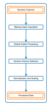
(a) Standard Preprocessing Pipeline

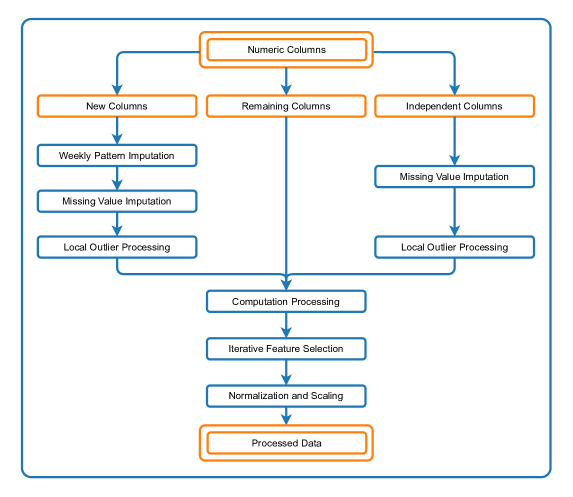
(b) Custom Preprocessing Pipeline

Figure 1: COVID Data Preprocessing Pipelines for (a) Standard and (b) Custom approaches

This study addresses these gaps by introducing a novel custom preprocessing pipeline (see Figure 1b) designed to address the unique challenges of COVID-19 datasets. The primary objective is to enhance data consistency and coherence through comprehensive exploration, meticulous cleaning, and effective preprocessing. The custom pipeline incorporates several innovative steps:

Weekly Pattern Imputation

Transforms weekly reported totals into daily updates by averaging the weekly sum and distributing it evenly across each day, thereby correcting summing errors and addressing reporting inconsistencies.

Local Outlier Processing

Uses a rolling window approach for local outlier detection, which accommodates local data variability rather than relying on standard global outlier detection methods.

Computation Processing

Calculates column values by leveraging inter-column dependencies, thereby preserving data consistency.

Iterative Feature Selection

Employs advanced techniques such as Permutation Feature Importance (PFI) [40], Mutual Information (MI) [41], Single Feature Impact (SFI) [14], and the Variance Inflation Factor (VIF) [42] to systematically eliminate redundant and collinear features while retaining the most significant ones. This approach refines the feature set by balancing predictive power, addressing multicollinearity, and improving overall model performance.

Our results show that all tested models benefit from the custom preprocessing pipeline, with non-linear models achieving the highest scores as anticipated. The consistent and stable performance across training, validation, and test sets highlights the novel contributions of this custom preprocessing pipeline in improving predictive accuracy and reliability. These findings offer valuable insights for researchers, policymakers, and healthcare professionals, supporting improved decision-making in pandemic management and future health crises.

The remainder of this paper is organized as follows: Section II outlines the data sources, preprocessing techniques, and machine learning models and evaluation strategies used in this study. Section III compares the model performance across different preprocessing pipelines and discusses the impact of various preprocessing techniques. Finally, Section IV summarizes the findings, highlights the contributions, and offers recommendations for future work.

II Data and Methodology

II-A Data

The dataset used in this study is sourced from Our World In Data (OWID) [2], and comprises over 400,000 rows and 67 columns, covering data from around the world. The dataset includes information from 244 countries, 6 continents, the European Union, and various income levels. Our analysis focuses specifically on India, using data collected from January 5, 2020, to August 11, 2024, amounting to 1,680 records.

The dataset includes one date column, four categorical columns (e.g., $iso\_code$, $location$, $continent$, and $tests\_units$), and 62 numeric columns that provide a detailed view of COVID-19 trends and influencing factors. Among the numeric columns, 12 are empty, 15 are constant, and 35 exhibit variability, which provides a rich source for analysis.

II-B Standard Preprocessing Pipeline

In the standard preprocessing pipeline (see Figure 1a), we applied traditional methods for dataset preparation. The process included the following steps:

II-B1 Extracting Numeric Features

We focused on numeric columns as categorical columns remained constant across countries and did not contribute to the analysis.

II-B2 Missing Value Imputation

We handled missing values using a two-step approach. Firstly, we applied linear interpolation and extrapolation to estimate the missing values. Then, we filled any remaining gaps with zero imputation. The orange line in Figure 5 visually illustrates how we applied this process to impute $positive\_rate$.

II-B3 Global Outlier Processing

We identified outliers using a z-score threshold of 2 and then processed them by applying linear interpolation. Figure 3a shows how we used this method for $new\_vaccinations$.

II-B4 Iterative Feature Selection

We systematically identified the most relevant features for our predictive model and addressed multicollinearity through iterative feature selection, as detailed in Algorithm 1. The key steps included:

Correlation Filtering

We removed features with correlations above 0.8 ($corr_{th}=0.8$) to minimise redundancy and multicollinearity. We also discarded constant features (zero correlations) and empty features (undefined correlations), because they do not provide useful information.

Calculating Importance Metrics

We assessed the importance of each remaining feature using three metrics:

• Permutation Feature Importance (PFI): Measures the impact on model performance when feature values are shuffled, reflecting overall predictive power.

• Mutual Information (MI): Quantifies the information a feature provides about the target, capturing both linear and non-linear dependencies.

• Single Feature Impact (SFI): Assesses the predictive power of each feature in isolation, offering a baseline view of its importance.

These metrics provided a comprehensive view of feature importance. PFI captured interactions, MI identified non-linear relationships, and SFI evaluated the individual predictive strength of each feature.

Variance Inflation Factor (VIF)

We quantified multicollinearity using the Variance Inflation Factor (VIF), defined as:

$$VIF_{j}=\frac{1}{1-R_{j}^{2}}$$ (1)

where $R_{j}^{2}$ is the coefficient of determination when regressing feature $j$ on all other features. The generally accepted thresholds for VIF are:

• $VIF=1$: No multicollinearity.

• $1<VIF<5$: Moderate multicollinearity, generally acceptable.

• $VIF>5$: High multicollinearity, potentially problematic.

We set a threshold of 10 to flag features for removal, balancing the need to address multicollinearity with maintaining a sufficient number of features for model stability and interpretability.

Iterative Removal of Features

We refined the feature set by iteratively removing features with high VIF and low combined importance:

• We identified features with VIF values exceeding the threshold.

• We removed the feature with the lowest combined importance score among those flagged.

Algorithm 1 Iterative Feature Selection

  Input: features, target

  Output: features

  $vif_{th}\leftarrow 10$

  $corr_{th}\leftarrow 0.8$

  Step 1: Correlation Filtering

  $features\leftarrow\text{CORR\_FILTER}(features,target,corr_{th})$

  repeat

     Step 2: Calculate Importance Metrics

     $pfi\leftarrow\text{PERM\_IMP}(features,target)$

     $mi\leftarrow\text{MUT\_INFO}(features,target)$

     $sfi\leftarrow\text{SINGLE\_FEAT\_IMPACT}(features,target)$

     Step 3: Compute VIF

     $vif\leftarrow\text{VIF}(features)$

     Step 4: Combine Importances

     $comb\_imp\leftarrow\text{COMB\_IMP}(pfi,mi,sfi)$

     Termination Condition:

     if $\max(vif)\leq vif_{th}$ then

        Return: features

     else

        Step 5: Identify and Remove Features

        $high\_vif\leftarrow\{f\mid vif[f]>vif_{th}\}$

        $imp_{min}\leftarrow\min(\{comb\_imp[f]\mid f\in high\_vif\})$

        for each $f\in high\_vif$ do

           if $comb\_imp[f]=imp_{min}$ then

              $features\leftarrow features\setminus\{f\}$ {Remove feature with high VIF and lowest importance}

              break

           end if

        end for

        Step 6: Regularization for Further Refinement

        $features\leftarrow\text{REFINE\_WITH\_REG}(features)$ {Drop features with zero coefficients}

     end if

  until $\max(vif)\leq vif_{th}$

Regularization for Further Refinement

We further refined the feature set by eliminating features with zero coefficients.

Termination Condition

The iterative process concluded when all remaining features had VIF values below the threshold, ensuring a relevant feature set with minimal redundancy.

II-B5 Normalization and Scaling

We standardized the shortlisted features to have a mean of zero and a standard deviation of one. This normalization ensured equal contribution of all features to model performance, facilitating effective comparison and analysis.

II-C Custom Preprocessing Pipeline

We designed the custom preprocessing pipeline (see Figure 1b) to enhance data quality and model performance through several tailored preprocessing steps. This section details the unique procedures we applied, the rationale behind them, and their impact on the data and model performance.

II-C1 Grouping Columns

We grouped columns into three categories to apply specialized preprocessing methods:

• New Columns: We identified columns such as $new\_cases$ and $new\_deaths$ as having weekly update patterns, which required specific handling to avoid bias.

• Independent Columns: We classified columns such as $new\_tests$, $new\_vaccinations$, $reproduction\_rate$, $people\_vaccinated$, $people\_fully\_vaccinated$, $total\_boosters$, and $stringency\_index$ as not exhibiting weekly patterns and we did not consider any computational dependencies for them.

• Remaining Columns: We designated the remaining columns as either constant or have computational dependencies.

II-C2 Preprocessing ‘New Columns’

For ‘New Columns’, we applied the following preprocessing methods:

Weekly Pattern Imputation

We corrected the weekly update pattern by redistributing total weekly values evenly across all days. This adjustment aimed to prevent bias, particularly in the $new\_deaths$ data, which showed weekly variations that could distort model predictions. Figure 2 visually represents the effectiveness of this imputation compared to the standard approach, highlighting the removal of bias introduced by weekly patterns.

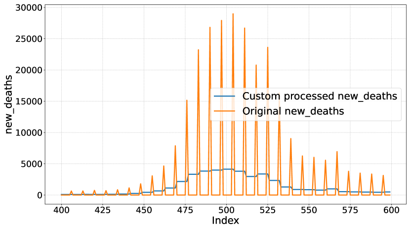
Figure 2: Comparison of Original vs. Custom Processed $new\_deaths$ Data (Zoomed-In View of Samples from index 400 to 600): Highlighting the Effectiveness of Weekly Pattern Imputation.

Missing Value Imputation

We handled missing values with linear interpolation followed by zero imputation, consistent with the standard pipeline approach to ensure comparability.

Local Outlier Processing

We addressed local extrema in time-series data by applying rolling z-scores with a 30-day window and a z-score threshold of 2. This approach effectively differentiated between genuine outliers and natural data variations, preserving critical data patterns. Figures 3 compare global and local outlier detection methods, demonstrating how the local approach preserved data variations and accurately detected outliers.

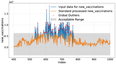
(a) Global outlier detection and processing

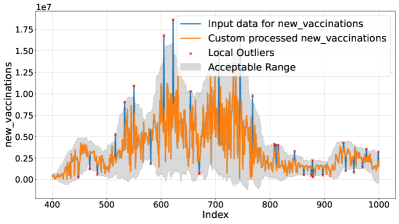
(b) Local outlier detection and processing

Figure 3: Comparison of outlier detection and winsorization techniques for the $new\_vaccinations$ column from index 400 to 1000. (a) Global outlier detection and processing with the standard pipeline, and (b) Local outlier detection and processing with the custom pipeline.

II-C3 Preprocessing ‘Independent Columns’

We applied the same preprocessing steps to ‘Independent Columns’ as those used for ‘New Columns’, except for weekly pattern imputation. This uniform treatment ensured consistency across different column types.

II-C4 Preprocessing ‘Remaining Columns’

For the ‘Remaining Columns’, we applied the following computation processing:

Computation Processing

We leveraged computational dependencies among columns to ensure consistency and resolve discrepancies. Figure 4 illustrates the dependencies and computation orders for the death-related columns. We processed $new\_deaths$ first, followed by $total\_deaths$ (using equation 3), $new\_deaths\_smoothed$ (using equation 6), and $new\_deaths\_per\_million$ (using equation 7) as they share the same processing order (order 2). Subsequently, we processed $total\_deaths\_per\_million$ and $new\_deaths\_smoothed\_per\_million$ (using equation 7) with processing order 3. Adhering to these manually determined but logically sequenced processing orders ensured both the consistency of computations and the integrity of the data.

Figure 5 compares the standard imputation method and our computation-based approach for the $positive\_rate$ column. While the standard pipeline imputed missing values with constant values (depicted by the orange line), our custom method calculated $positive\_rate$ using equation 4. This approach, which relies on processed $new\_cases$ and $new\_tests$ values, delivered accurate and consistent results that captured natural variations (particularly within the shaded region) rather than relying on constant extrapolation.

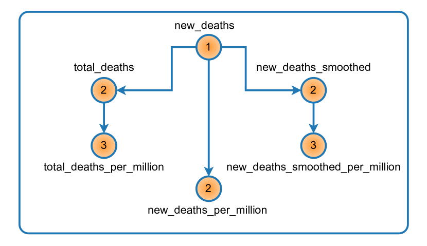
Figure 4: Column dependency graph for the ‘death’ columns with processing orders

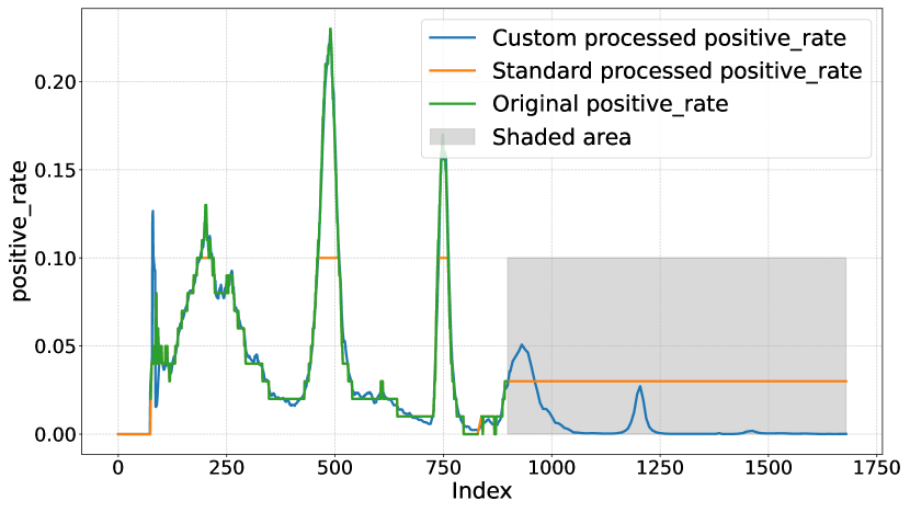
Figure 5: Plotting for computation processing of $positive\_rate$ column

$new$ Columns

Computed as the difference between $total$ column values at the current index $t$ and the previous index $t-1$:

$$X_{new}^{t}=\begin{cases}X_{total}^{t}&{\text{, if }}t=0\\ X_{total}^{t}-X_{total}^{t-1}&{\text{, if }}t>0\end{cases}$$ (2)

We created a new column $new\_people\_vaccinated$ in our custom approach and used this equation to compute $new\_people\_vaccinated$ from $people\_vaccinated$.

$total$ Columns

Computed as the cumulative sum of the corresponding $new$ column:

$$X_{total}^{t}=\sum_{i=0}^{t}X_{new}^{i}$$ (3)

This equation calculated $total$ columns from their corresponding $new$ columns, such as $new\_cases$, $new\_deaths$, $new\_tests$, and $new\_vaccinations$.

$positive\_rate$

Represented the proportion of positive test results among the total tests conducted, calculated from $new\_cases$ and $new\_tests$:

$$X_{positive\_rate}^{t}=\frac{\sum_{i=0}^{6}\frac{X_{new\_cases}^{t-i}}{X_{new\_tests}^{t-i}}}{7}$$ (4)

Refer to Figure 5 for a visualization of the $positive\_rate$ computation.

$tests\_per\_case$

Represented the number of tests conducted per confirmed case of COVID-19, calculated as the reciprocal of $positive\_rate$:

$$X_{tests\_per\_case}^{t}=\frac{1}{X_{positive\_rate}^{t}}$$ (5)

$smoothed$ Column

Calculated as the 7-day moving average of the corresponding $raw$ column:

$$X_{smoothed}^{t}=\frac{\sum_{i=0}^{6}X_{raw}^{t-i}}{7}$$ (6)

This equation is applied to columns such as $new\_cases$, $new\_deaths$, $new\_tests$, $new\_vaccinations$, and $new\_people\_vaccinated$.

$per\_million$ Column

Calculated by dividing each $raw$ value by the total population and multiplying by one million:

$$X_{per\_million}^{t}=\frac{X_{raw}^{t}\times 10^{6}}{population}$$ (7)

This equation was used to derive the $per\_million$ values for columns such as $total\_cases$, $new\_cases$, $total\_deaths$, $new\_deaths$, $new\_deaths\_smoothed$, $new\_cases\_smoothed$, and $new\_vaccinations\_smoothed$.

$per\_thousand$ Column

Calculated by dividing each $raw$ value by the total population and multiplying by one thousand:

$$X_{per\_thousand}^{t}=\frac{X_{raw}^{t}\times 10^{3}}{population}$$ (8)

This formula was used to derive $per\_thousand$ values for columns such as $total\_tests$, $new\_tests$, and $new\_tests\_smoothed$.

$per\_hundred$ Column

Calculated by dividing each $raw$ value by the total population and multiplying by one hundred:

$$X_{per\_hundred}^{t}=\frac{X_{raw}^{t}\times 10^{2}}{population}$$ (9)

This formula was used to derive $per\_hundred$ values for columns such as $total\_vaccinations$, $people\_vaccinated$, $people\_fully\_vaccinated$, $total\_boosters$, and $new\_people\_vaccinated\_smoothed$.

After preprocessing, we split the dataset into training, validation, and test sets. The training data then underwent iterative feature selection, followed by normalization and scaling, using the same methods as in the standard pipeline.

II-D Model Training and Evaluation

We trained and evaluated ten regression models using the preprocessed datasets from both pipelines: Linear Regression, Ridge Regression, Lasso Regression, ElasticNet Regression, Support Vector Regression (SVR), Random Forest Regression, Gradient Boosting Regression, Decision Tree Regression, K-Nearest Neighbors Regression (KNN), and Neural Network Regression (Multilayer Perceptron). To prevent overfitting and optimize model performance, we applied 5-fold cross-validation and hyperparameter tuning.

II-D1 Evaluation Results

We assessed the models’ performance using three key metrics: $RMSE$, $R^{2}$, and RMSE Variance.

$RMSE$ (Root Mean Squared Error) and $R^{2}$ (Coefficient of Determination) are standard metrics for evaluating model accuracy and explanatory power. To assess the consistency of a model’s performance across different data splits, we introduced an additional metric, RMSE Variance. This metric measures how consistently a model performs across the training, validation, and testing datasets. It is computed as follows:

$$\textit{RMSE Variance}=\frac{1}{n}\sum_{i=1}^{n}\left(RMSE_{i}-\overline{RMSE}\right)^{2}$$ (10)

where $RMSE_{i}$ represented the $RMSE$ for the training, validation, and testing datasets, $\overline{RMSE}$ was the mean $RMSE$ across these datasets, and $n$ was the total number of datasets (which is 3 in this case). RMSE Variance thus measured the variance of these three $RMSE$ values. A lower RMSE Variance indicated consistent performance across datasets, suggesting better generalizability and robustness, while a higher variance might have indicated potential overfitting or poor generalization.

By employing these metrics, we gained insights into the overall accuracy, generalization capability, and performance consistency of the models across different stages. The evaluations were conducted separately for the standard and custom preprocessing pipelines, enabling a direct comparison of the impact each pipeline had on model performance.

II-E Implementation Details

The implementation was carried out in Python using Jupyter Notebooks, executed on Google Colab in a CPU environment. The complete notebook runs in approximately one hour on a standard Google Colab CPU instance (Intel Xeon CPU @ 2.20GHz with 12.6 GB of RAM).

II-E1 Source Code

The complete source code for this study is available in a Jupyter Notebook and can be accessed through the Github repository.

III Results and Discussion

III-A Model Performance Evaluation

This section presents and analyzes the performance metrics of various regression models evaluated using standard and custom preprocessing pipelines.

III-A1 Test Results: Test RMSE and R²

Table I summarizes the evaluation results for each model in both pipelines (for further details, see the GitHub repository). The custom preprocessing pipeline consistently outperformed the standard one across all models. The MLPRegressor with the custom pipeline achieved the best performance, recording an RMSE of 66.556 and an R² of 0.991. In contrast, the DecisionTreeRegressor in the standard pipeline had the best results among the standard models, with an RMSE of 222.858 and an R² of 0.817. The custom pipeline’s lower RMSE and higher R² values indicate superior predictive accuracy and a better model fit across the board.

TABLE I: Performance Metrics for Various Models Using Standard and Custom Pipelines

Pipeline	Model	Test RMSE	Test R²	RMSE Variance
Standard	DecisionTreeRegressor	222.858	0.817	776.666
	RandomForestRegressor	238.373	0.790	3740.121
	GradientBoostingRegressor	242.053	0.784	1762.070
	SVR	278.971	0.713	746.453
	KNeighborsRegressor	366.496	0.504	8318.961
	Ridge	406.051	0.391	1437.239
	ElasticNet	406.054	0.391	1437.262
	LinearRegression	406.144	0.391	1438.698
	Lasso	406.185	0.391	1441.244
	MLPRegressor	419.340	0.350	13739.921
Custom	MLPRegressor	66.556	0.991	52.125
	KNeighborsRegressor	84.510	0.985	210.551
	GradientBoostingRegressor	86.926	0.984	108.862
	RandomForestRegressor	144.046	0.956	2126.466
	DecisionTreeRegressor	146.775	0.955	1768.430
	SVR	208.737	0.908	766.496
	Ridge	406.188	0.652	6.828
	LinearRegression	406.204	0.652	6.889
	Lasso	406.322	0.652	6.967
	ElasticNet	406.342	0.652	6.772

III-A2 Generalizability: Overfitting and Underfitting

The consistency of model performance across different datasets was assessed using RMSE variance, where lower values indicate better generalization. Models from the custom pipeline generally exhibited lower RMSE variances, suggesting they were less prone to overfitting. For instance, the MLPRegressor in the custom pipeline demonstrated high stability with an RMSE variance of 52.125, while the same model in the standard pipeline showed significant instability with an RMSE variance of 13,739.921, indicating potential overfitting.

III-A3 Impact of Weekly Pattern Imputation

The dataset initially displayed a weekly update pattern for $new\_deaths$, with zeros reported for six days and the total on the seventh day, This pattern could bias models by distorting the underlying trend. The custom pipeline addressed this by redistributing the weekly totals across all days, which enhanced model performance. Although we tested $new\_deaths\_smoothed$ as a target variable, results indicated that the standard pipeline performed unusually well with this target due to global outlier processing. This processing stripped away essential data variations, inflating performance metrics artificially, as shown in Figure 3a. This finding underscores the importance of preserving data variability for accurate model evaluation.

III-A4 Global vs. Local Outlier Processing

Global outlier detection and processing, using fixed z-score thresholds, often fails to capture local data variability. Our findings suggest that local outlier detection, which adapts thresholds contextually, better preserves data integrity and improves model accuracy. This approach is preferred for time-series data like COVID-19.

III-A5 Computation Processing and Feature Stability

Computation processing ensured consistent relationships between features, leading to more stable models. Early iterations of the feature selection exhibited infinite Variance Inflation Factor (VIF) values for most columns (see the GitHub repository), indicating perfectly consistent feature relationships. In contrast, the standard pipeline showed finite VIF values, reflecting less consistent feature dependencies and contributing to less reliable model performance.

III-A6 Iterative Feature Selection and its Impact

Iterative feature selection was employed to refine the feature set, reducing the number of numeric features from 34 (excluding the target) to 5 in the custom pipeline and 7 in the standard pipeline. Despite this reduction, the custom pipeline achieved higher accuracy and consistency, demonstrating the effectiveness of the feature selection approach. The iterative process effectively managed feature relationships and minimized multicollinearity, as indicated by VIF values below 5 (see Table II) in both pipelines. However, the custom pipeline’s features exhibited superior combined importance scores, contributing to its enhanced performance.

Feature Importance Scores

Table II compares the combined feature importance scores and VIF values for features selected by the standard and custom pipelines. This table highlights the differences in feature importance and multicollinearity between the pipelines. Features in the custom pipeline have significantly higher combined importance scores compared to those in the standard pipeline, reflecting more effective data processing. For instance, the $stringency\_index$ was shortlisted by both pipelines, but its combined importance score was 0.160 in the standard pipeline compared to 1.128 in the custom pipeline. This discrepancy underscores the substantial performance improvement achieved with the custom pipeline.

TABLE II: Combined Feature Importance Scores and VIF Values for Shortlisted Features in Standard and Custom Pipelines

Pipeline	Features	Combined Importance	VIF
Standard	$new\_cases\_per\_million$	0.807	1.096
	$new\_deaths\_smoothed$	0.353	3.197
	$total\_cases\_per\_million$	0.328	3.013
	$tests\_per\_case$	0.242	3.131
	$new\_people\_vaccinated\_smoothed$	0.237	4.718
	$new\_vaccinations$	0.190	4.998
	$stringency\_index$	0.160	4.852
Custom	$new\_cases$	2.161	1.570
	$total\_deaths\_per\_million$	1.676	2.464
	$stringency\_index$	1.128	2.696
	$tests\_per\_case$	1.001	1.395
	$new\_people\_vaccinated$	0.708	1.464

The custom pipeline’s features exhibited infinite VIF values, indicating stable relationships, whereas the standard pipeline’s finite VIF values suggested less effective feature selection.

III-B Summary and Recommendations

Weekly Pattern Imputation

Redistributing weekly totals to daily updates improved model performance by preserving data integrity and minimizing bias. We recommend this approach for accurate and reliable predictions.

Local Outlier Processing

Local outlier processing effectively identifies and handles outliers while preserving data variance. This method is preferred over global outlier processing for consistent and accurate modelling.

Computation Processing

The custom pipeline’s computation processing ensured perfect feature consistency, leading to superior model performance. Identifying and leveraging computational dependencies is essential for accurate imputation and modelling.

Iterative Feature Selection

The custom pipeline’s iterative feature selection, despite using fewer features, achieved higher accuracy and consistency due to the effective management of feature relationships and multicollinearity. This approach is recommended for optimizing feature sets in predictive modelling.

In conclusion, the custom pipeline’s tailored approaches in imputation, outlier processing, computation, and feature selection resulted in more robust and accurate predictive models. These methods not only demonstrated superiority over the standard pipeline but also have broad applicability to other preprocessing and machine learning tasks. Adopting these custom approaches can enhance predictive modelling across various domains and datasets.

IV Conclusion

This study highlights the essential role of a tailored data preprocessing pipeline in enhancing the accuracy and reliability of COVID-19 mortality predictions. By redistributing weekly totals for the target variable ($new\_deaths$), utilizing local outlier detection to preserve data variance, leveraging computational dependencies, and employing iterative feature selection, the custom pipeline significantly outperformed the standard approach. Specifically, the MLPRegressor model with the custom pipeline achieved an RMSE of 66.556, an R² of 0.991, and an RMSE variance of 52.125, compared to the best standard pipeline results with the DecisionTreeRegressor, which recorded an RMSE of 222.858, an R² of 0.817, and an RMSE variance of 776.666, highlighting the substantial improvement. These improvements demonstrate the effectiveness of custom preprocessing, particularly for time-series data with distinct patterns and outliers. Although this study focuses on data from India, future research should apply this pipeline to datasets from other countries, where additional dependencies may need to be addressed. The techniques of local outlier detection, iterative feature selection, and RMSE variance evaluation are broadly applicable and can enhance data integrity, consistency, and model performance across diverse domains and datasets.

References

- [1] M. Andrews, B. Areekal, K. Rajesh, J. Krishnan, R. Suryakala, B. Krishnan, C. Muraly, and P. Santhosh, “First confirmed case of covid-19 infection in india: A case report,” The Indian journal of medical research, vol. 151, no. 5, p. 490, 2020.
- [2] E. Mathieu, H. Ritchie, L. Rodés-Guirao, C. Appel, C. Giattino, J. Hasell, B. Macdonald, S. Dattani, D. Beltekian, E. Ortiz-Ospina, and M. Roser, “Coronavirus pandemic (covid-19),” Our World in Data, 2020. https://ourworldindata.org/coronavirus.
- [3] A. L. Mueller, M. S. McNamara, and D. A. Sinclair, “Why does covid-19 disproportionately affect older people?,” Aging (albany NY), vol. 12, no. 10, p. 9959, 2020.
- [4] D. R. Petretto and R. Pili, “Ageing and covid-19: What is the role for elderly people?,” 2020.
- [5] C. An, H. Lim, D.-W. Kim, J. H. Chang, Y. J. Choi, and S. W. Kim, “Machine learning prediction for mortality of patients diagnosed with covid-19: a nationwide korean cohort study,” Scientific reports, vol. 10, no. 1, p. 18716, 2020.
- [6] F. Rustam, A. A. Reshi, A. Mehmood, S. Ullah, B.-W. On, W. Aslam, and G. S. Choi, “Covid-19 future forecasting using supervised machine learning models,” IEEE access, vol. 8, pp. 101489–101499, 2020.
- [7] A. K. Das, S. Mishra, and S. S. Gopalan, “Predicting covid-19 community mortality risk using machine learning and development of an online prognostic tool,” PeerJ, vol. 8, p. e10083, 2020.
- [8] A. L. Booth, E. Abels, and P. McCaffrey, “Development of a prognostic model for mortality in covid-19 infection using machine learning,” Modern Pathology, vol. 34, no. 3, pp. 522–531, 2021.
- [9] S. Subudhi, A. Verma, A. B. Patel, C. C. Hardin, M. J. Khandekar, H. Lee, D. McEvoy, T. Stylianopoulos, L. L. Munn, S. Dutta, et al., “Comparing machine learning algorithms for predicting icu admission and mortality in covid-19,” NPJ digital medicine, vol. 4, no. 1, p. 87, 2021.
- [10] M. Mahdavi, H. Choubdar, E. Zabeh, M. Rieder, S. Safavi-Naeini, Z. Jobbagy, A. Ghorbani, A. Abedini, A. Kiani, V. Khanlarzadeh, et al., “A machine learning based exploration of covid-19 mortality risk,” Plos one, vol. 16, no. 7, p. e0252384, 2021.
- [11] D. Krithika and K. Rohini, “Comparative intrepretation of machine learning algorithms in predicting the cardiovascular death rate for covid-19 data,” in 2021 International Conference on Computational Intelligence and Knowledge Economy (ICCIKE), pp. 394–400, IEEE, 2021.
- [12] H. Wang, M. J. Bah, and M. Hammad, “Progress in outlier detection techniques: A survey,” Ieee Access, vol. 7, pp. 107964–108000, 2019.
- [13] E. Rahm, H. H. Do, et al., “Data cleaning: Problems and current approaches,” IEEE Data Eng. Bull., vol. 23, no. 4, pp. 3–13, 2000.
- [14] I. Guyon and A. Elisseeff, “An introduction to variable and feature selection,” Journal of machine learning research, vol. 3, no. Mar, pp. 1157–1182, 2003.
- [15] J. Bergstra, R. Bardenet, Y. Bengio, and B. Kégl, “Algorithms for hyper-parameter optimization,” Advances in neural information processing systems, vol. 24, 2011.
- [16] L. Winston, M. McCann, G. Onofrei, et al., “Exploring socioeconomic status as a global determinant of covid-19 prevalence, using exploratory data analytic and supervised machine learning techniques: Algorithm development and validation study,” JMIR Formative Research, vol. 6, no. 9, p. e35114, 2022.
- [17] S. Moustakidis, C. Kokkotis, D. Tsaopoulos, P. Sfikakis, S. Tsiodras, V. Sypsa, T. E. Zaoutis, and D. Paraskevis, “Identifying country-level risk factors for the spread of covid-19 in europe using machine learning,” Viruses, vol. 14, no. 3, p. 625, 2022.
- [18] T. Sha’ban, H. Hailat, A. Nawafleh, and H. Najadat, “Assessing the effectiveness of covid-19/sars-cov-2 vaccinations in terms of mortality rates,” in 2023 14th International Conference on Information and Communication Systems (ICICS), pp. 1–6, IEEE, 2023.
- [19] M. Eryılmaz, Ö. Ertan, F. Yalçınkaya, and E. Kara, “A prediction study about the pandemic era based on machine learning methods,” International Journal on Recent and Innovation Trends in Computing and Communication, vol. 9, no. 12, p. 01–07, 2021.
- [20] M. Pourhomayoun and M. Shakibi, “Predicting mortality risk in patients with covid-19 using machine learning to help medical decision-making,” Smart health, vol. 20, p. 100178, 2021.
- [21] I. N. Schrarstzhaupt, M. A. d. S. Bragatte, L. Kawano-Dourado, L. R. d. Oliveira, G. F. Vieira, F. A. Diaz-Quijano, and M. Fontes-Dutra, “Interactive monitoring dashboards for the covid-19 pandemic in the world anticipating waves of the disease in brazil with the use of open data,” Revista Brasileira de Epidemiologia, vol. 27, p. e240004, 2024.
- [22] K. A. Beattie, “Worldwide bayesian causal impact analysis of vaccine administration on deaths and cases associated with covid-19: A bigdata analysis of 145 countries,” Department of Political Science University of Alberta Alberta, Canada, 2021.
- [23] C. Hu, Z. Liu, Y. Jiang, O. Shi, X. Zhang, K. Xu, C. Suo, Q. Wang, Y. Song, K. Yu, et al., “Early prediction of mortality risk among patients with severe covid-19, using machine learning,” International journal of epidemiology, vol. 49, no. 6, pp. 1918–1929, 2020.
- [24] I. U. Khan, N. Aslam, M. Aljabri, S. S. Aljameel, M. M. A. Kamaleldin, F. M. Alshamrani, and S. M. B. Chrouf, “Computational intelligence-based model for mortality rate prediction in covid-19 patients,” International journal of environmental research and public health, vol. 18, no. 12, p. 6429, 2021.
- [25] M. Zubair, M. Asif Iqbal, A. Shil, E. Haque, M. Moshiul Hoque, and I. H. Sarker, “An efficient k-means clustering algorithm for analysing covid-19,” in Hybrid Intelligent Systems: 20th International Conference on Hybrid Intelligent Systems (HIS 2020), December 14-16, 2020, pp. 422–432, Springer, 2021.
- [26] Y. Xia, P. Zhu, and Z. Zhou, “Analysis and prediction of covid-19 based on machine learning,” Highlights in Science, Engineering and Technology, vol. 38, pp. 725–735, 2023.
- [27] J. M. Jerez, I. Molina, P. J. García-Laencina, E. Alba, N. Ribelles, M. Martín, and L. Franco, “Missing data imputation using statistical and machine learning methods in a real breast cancer problem,” Artificial intelligence in medicine, vol. 50, no. 2, pp. 105–115, 2010.
- [28] G. E. Batista and M. C. Monard, “An analysis of four missing data treatment methods for supervised learning,” Applied artificial intelligence, vol. 17, no. 5-6, pp. 519–533, 2003.
- [29] A. Vaid, S. Somani, A. J. Russak, J. K. De Freitas, F. F. Chaudhry, I. Paranjpe, K. W. Johnson, S. J. Lee, R. Miotto, F. Richter, et al., “Machine learning to predict mortality and critical events in a cohort of patients with covid-19 in new york city: model development and validation,” Journal of medical Internet research, vol. 22, no. 11, p. e24018, 2020.
- [30] M. E. Chowdhury, T. Rahman, A. Khandakar, S. Al-Madeed, S. M. Zughaier, S. A. Doi, H. Hassen, and M. T. Islam, “An early warning tool for predicting mortality risk of covid-19 patients using machine learning,” Cognitive Computation, pp. 1–16, 2021.
- [31] P. Pan, Y. Li, Y. Xiao, B. Han, L. Su, M. Su, Y. Li, S. Zhang, D. Jiang, X. Chen, et al., “Prognostic assessment of covid-19 in the intensive care unit by machine learning methods: model development and validation,” Journal of medical Internet research, vol. 22, no. 11, p. e23128, 2020.
- [32] V. P. K. Turlapati and M. R. Prusty, “Outlier-smote: A refined oversampling technique for improved detection of covid-19,” Intelligence-based medicine, vol. 3, p. 100023, 2020.
- [33] A. N. Brzezińska and C. Horyń, “Outliers in covid 19 data based on rule representation-the analysis of lof algorithm,” Procedia Computer Science, vol. 192, pp. 3010–3019, 2021.
- [34] N. Herawati, K. Nisa, and S. Saidi, “Implementation of the trimmed k-means clustering method in mapping the distribution of covid-19 in indonesia,” in AIP Conference Proceedings, vol. 2563, AIP Publishing, 2022.
- [35] K. Moulaei, M. Shanbehzadeh, Z. Mohammadi-Taghiabad, and H. Kazemi-Arpanahi, “Comparing machine learning algorithms for predicting covid-19 mortality,” BMC medical informatics and decision making, vol. 22, no. 1, pp. 1–12, 2022.
- [36] T. W. Tulu, T. K. Wan, C. L. Chan, C. H. Wu, P. Y. M. Woo, C. Z. S. Tseng, A. Vodencarevic, C. Menni, and K. H. K. Chan, “Machine learning-based prediction of covid-19 mortality using immunological and metabolic biomarkers,” BMC Digital Health, vol. 1, no. 1, p. 6, 2023.
- [37] E. Gambhir, R. Jain, A. Gupta, and U. Tomer, “Regression analysis of covid-19 using machine learning algorithms,” in 2020 International conference on smart electronics and communication (ICOSEC), pp. 65–71, IEEE, 2020.
- [38] S. García, S. Ramírez-Gallego, J. Luengo, J. M. Benítez, and F. Herrera, “Big data preprocessing: methods and prospects,” Big data analytics, vol. 1, pp. 1–22, 2016.
- [39] V. Gudivada, A. Apon, and J. Ding, “Data quality considerations for big data and machine learning: Going beyond data cleaning and transformations,” International Journal on Advances in Software, vol. 10, no. 1, pp. 1–20, 2017.
- [40] U. Michelucci, “Feature importance and selection,” in Fundamental Mathematical Concepts for Machine Learning in Science, pp. 229–242, Springer, 2024.
- [41] A. Kraskov, H. Stögbauer, and P. Grassberger, “Estimating mutual information,” Physical Review E—Statistical, Nonlinear, and Soft Matter Physics, vol. 69, no. 6, p. 066138, 2004.
- [42] W. H. Greene, Econometric analysis. Pearson Education India, 2003.