The evolution of inharmonicity and noisiness in contemporary popular music

Abstract

Much of Western classical music uses instruments based on acoustic resonance. Such instruments produce harmonic or quasi-harmonic sounds. On the other hand, since the early 1970s, popular music has largely been produced in the recording studio. As a result, popular music is not bound to be based on harmonic or quasi-harmonic sounds. In this study, we use modified MPEG-7 features to explore and characterise the way in which the use of noise and inharmonicity has evolved in popular music since 1961. We set this evolution in the context of other broad categories of music, including Western classical piano music, Western classical orchestral music, and musique concrète. We propose new features that allow us to distinguish between inharmonicity resulting from noise and inharmonicity resulting from interactions between relatively discrete partials. When the history of contemporary popular music is viewed through the lens of these new features, we find that the period since 1961 can be divided into three phases. From 1961 to 1972, there was a steady increase in inharmonicity but no significant increase in noise. From 1972 to 1986, both inharmonicity and noise increased. Then, since 1986, there has been a steady decrease in both inharmonicity and noise to today’s popular music which is significantly less noisy but more inharmonic than the music of the sixties. We relate these observed trends to the development of music production practice over the period and illustrate them with focused analyses of certain key artists and tracks.

1 Introduction

Most musical instruments that perform Western classical music are based on the acoustic resonance principle. Such instruments produce harmonic or quasi-harmonic complex tones. In contemporary popular music, the means of production are more diversified. Drums play a key role, and they do not typically produce quasi-harmonic complex tones. Instruments may be based on electronic or digital sound production techniques. The instruments’ outputs may be heavily processed with effects. Musicians may not even use instruments and produce the entirety of the music on a computer. As a result, given a contemporary popular music track, it is possible that the description of the corresponding signal using quasi-harmonic complex tones is unsuitable.

In the spectral domain, a quasi-harmonic complex tone may be described as a series of partials whose frequency values are near multiples of one frequency value (the fundamental). There are at least two ways audio content may diverge from being quasi-harmonic: as exemplified in Lavengood, (2017, p. 22), the energy may not be centered around partials, in which case the signal may be described as ‘noisy’; or, as exemplified in Lavengood, (2017, p. 24), the partial frequency values may not be harmonically related, in which case the tone may be described as ‘inharmonic’.

In this paper, we trace the evolution over time of the relative amounts of inharmonicity and noise in various audio datasets. Our main focus is contemporary popular music (CPM), but we also compare this class of music with Western classical piano music, Western orchestral music, and music concrète.

One key conclusion of this study is that contemporary popular music is more inharmonic than the music from the three other datasets considered. Our diachronic analysis of the evolution of noisiness and inharmonicity in CPM leads to the conclusion that, between 1961 and 1986, recorded music evolved in a general direction that goes from acoustic, tonal instruments playing content from a musical score (or, at least, that can be transcribed to a score), to heavily processed, noisy, and inharmonic content made in the recording studio and including drums. In more recent decades, music has become slightly more harmonic.

The remainder of this paper is structured as follows. The core content of the study can be found in sections 3 and 4 (the ‘core sections’). Section 3 describes the datasets and the signal features used in the study. Section 4 presents the results of the analysis. Sections 5 to 11 elaborate on several notions introduced in the core sections. Section 5 reflects on the relationship between the means of production and the produced music. It elaborates on the reasoning that led to examining noise and inharmonicity in contemporary popular music. Section 6 details characteristics of the signal that influence the inharmonic character of the music, discusses the link between inharmonicity and acoustic beating (in other words the acoustical ‘grit’), and substantiates the definition of inharmonicity we use in the core sections. Section 7 details the reasoning leading to the definition of ‘noisiness’ we use in the core sections. Section 8 addresses the influence of the recording medium and remastering processes. Section 9 relates the results from the core sections to those of previous diachronic studies. Section 10 details the influence of the psychoacoustic weighting used in the core sections. Section 11 presents detailed analyses of specific music tracks from the perspective proposed in the core sections. The paper concludes by summarising the findings from all sections.

2 Background and motivation

A defining property of a harmonic tone is that it has a fundamental frequency or $f_{0}$. A classic music information retrieval task consists in estimating the fundamental frequency of a sound, often taken as a synonym for ‘pitch tracking’ or ‘pitch estimation’ (Kim et al.,, 2018; Riou et al.,, 2023). The models performing such tasks are trained on harmonic or quasi-harmonic audio. For instance, Riou et al., (2023) uses MIR-1K, a dataset of quasi-harmonic samples (Hsu and Jang,, 2009) and MDB-stem-synth, a dataset of ‘exact multiples of the $f_{0}$’ (Salamon et al.,, 2017).

Another classic music information retrieval task is audio-to-MIDI alignment (Raffel and Ellis,, 2016), in which MIDI files are aligned to a corresponding audio content. MIDI files have been referred to as symbolic ‘versions’ of pieces of music (Ewert et al.,, 2012; Raffel and Ellis,, 2016), a ‘transcription’ (Raffel,, 2016; Turetsky and Ellis,, 2003; Benetos et al.,, 2018) of the pitched content of the music. Such content has been characterised as ‘harmonic’ (Ono et al.,, 2008) and likely to being played with ‘harmonic instruments’ (Ewert et al.,, 2014).

In the pitch tracking and audio-to-midi alignment tasks, pitched content is generally considered harmonic or quasi-harmonic. Yet, interaction with actual professional music production may show a different picture. For example, Figure 1 shows the power spectrum of one bass ‘note’ in the 2023 track ‘¡Fire!’ by Primaal. Primaal is a brand of the Hyper Music production company mentioned by Deruty et al., (2022). In 2022 and 2023, Primaal authored music for commercials commissioned by brands such as L’Oréal, Adidas, Vichy, Honda, GoPro, and Chanel. Therefore, it is possible to consider that Primaal’s production reflects an existing trend in the music industry. We write ‘note’ in scare-quotes, as its content is not harmonic even though it provides an impression of pitch. This example is not unique. In Primaal’s production, many other parts provide an impression of pitch while not featuring harmonic content.

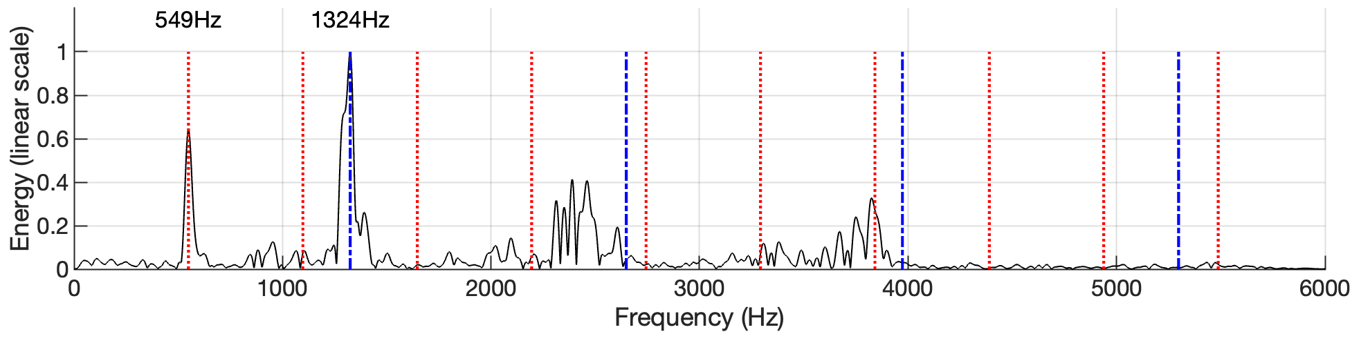
Figure 1: Power spectrum values for the first bass ‘note’ in Primaal’s ‘¡Fire!’. The vertical red and blue lines represent the fundamental and expected positions of the harmonics for the main two spectral peaks.

There, therefore, seems to be a discrepancy between such examples of the use of inharmonicity in real-world music production and what appears to be the standard view within music information retrieval that pitched content corresponds to harmonic tones. This discrepancy provides motivation for exploring the extent to which pitched elements in CPM are harmonic.

3 Methods

3.1 Datasets

In this study, we use the following four datasets of stereo audio tracks.

1. The popular music dataset, or ‘BEA dataset’, contains 30435 tracks released between 1961 and 2022. There are at least 460 tracks for each year. This dataset is an extension of the dataset used by Deruty and Pachet, (2015). The choice of tracks for the datasets stems from the ‘Best Ever Albums’ website, a review aggregator that proposes the best-rated albums for each year of production. The ratings are dynamic: new reviews may modify an album’s ranking, making the dataset a specific snapshot at the time of writing. The dataset indiscriminately involves original and remastered versions. The influence of the remastering process is discussed in section 8.

2. The piano dataset contains 4600 piano audio tracks from various sources, including Alpha’s ‘Schumann Project’, Ciccolini’s complete EMI recordings, and Brendel’s complete Decca recordings. Tracks from this dataset range from the Viennese Classical era to the early 20^th century. Different interpretations of the same original score may be found in the dataset.

3. The orchestra dataset contains 10800 orchestral and opera tracks from various sources, including Deutsche Grammophon’s ‘Classical Gold’, ‘The History of Classical Music’, Decca’s ‘55 Great Vocal Recitals’ and ‘Ultimate Boxset’ series. Tracks in this dataset range from the Baroque era to the early 20^th century. Again, different interpretations of the same original score may be found in the dataset.

4. The musique concrète dataset consists of 1000 tracks from composers related to Pierre Schaeffer’s school of thought by either having directly collaborated with him or having produced music at INA/GRM in Paris. It includes music by Pierre Henry, Bernard Parmegiani, Denis Dufour, and François Bayle.

3.2 Features

3.2.1 HR-inharmonicity

To measure inharmonicity, we use the Matlab R2022b implementation of the MPEG-7 feature HarmonicRatio. HarmonicRatio has been described as measuring ‘the proportion of harmonic components within the power spectrum’ (ISO,, 2001, p. 36), and ‘the ratio of harmonic power to total power’ (Moreau et al.,, 2006, p. 33). To our knowledge, HarmonicRatio is the only feature in the literature that measures the proportion of harmonic components in the general case. Features such as Inharmonicity in Peeters, (2004, p.17) measure ‘the […] divergence from a purely harmonic signal’ and can only be measured in relation to a single complex tone. HarmonicRatio derives from the normalised auto-correlation of the signal. The normalisation is performed so that the auto-correlation at zero lag equals one. The feature output is the maximum value of the normalised auto-correlation after the first zero-crossing. HarmonicRatio assumes values between 0 and 1, with harmonic complex tones resulting in 1. As we want to measure inharmonicity, we use a feature called HR-inharmonicity, defined as $1-HarmonicRatio$. Section  6 elaborates on the relationship between different aspects of the signal and HR-inharmonicity.

Patterson et al., (1996) and Yost, (1996, 1997) have argued that the ‘first peak of the auto-correlation function’ can be used to evaluate the ‘saliency or the strength of pitch of complex sounds’—in other words, the perceptual impression of pitch strength. The matter was further investigated by Shofner and Selas, (2002). The illustrations in Yost, (1996, p. 3330) and Shofner and Selas, (2002, p. 439) show without ambiguity that the ‘first peak of the auto-correlation function’ is the maximum value of the normalised auto-correlation after the first zero-crossing—that is, what the MPEG-7 standard designates as HarmonicRatio (ISO,, 2001; Moreau et al.,, 2006). One of our main concerns in this study is with quantifying the degree to which a signal deviates from being harmonic. However, as HarmonicRatio can be used to gauge the strength of pitch, the properties of the signal that we find to result in lower (or higher) HarmonicRatio values may also lead to a corresponding decrease (or increase) in the perceived strength of pitch.

3.2.2 Peak prominence and noisiness

Features have been proposed to measure the ‘noisiness’ of the signal, such as spectral flatness (Peeters,, 2004) and AudioSpectrumFlatnessType (ISO,, 2001). However, the two features are sensitive to the overall envelope of the spectrum: music and pink noise result in comparable spectral flatness values, which defeats the purpose of measuring ‘noisiness’. We introduce a new metric derived from spectral flatness and AudioSpectrumFlatnessType that is robust to the overall spectral profile. We refer to this feature as peak prominence and to the inverse of peak prominence as noisiness. Section 7 details the elaboration of the metric.

3.2.3 Inharmonicity

Inharmonicity has been defined as ‘the departure in frequency from the harmonic modes of vibration’ (Young,, 1952), and ‘the deviation of a set of frequencies from an exact harmonic series’ (Campbell,, 2001). A further distinction can be observed, between ‘inharmonic sounds which have little if any relevance for music (e.g., white or pink noise)’ (Schneider and Frieler,, 2009) and ‘coherent’ inharmonic signals, which ‘sound as stable and smooth as harmonic signals’ (de Boer,, 1956). In other words, inharmonicity can be the result of either inharmonic partial relations or noise. Section 6.6 elaborates on the relationship between noise and inharmonicity.

HR-inharmonicity and peak prominence are not independent. Adding white noise to a harmonic complex tone does not change the partial positions, yet it lowers the maximum value of the normalised auto-correlation after the first zero-crossing, resulting in lower HR-inharmonicity values (see section 6.6 for more details). To measure inharmonicity independently from ‘noisiness’, we perform a PCA on the distribution of HR-inharmonicity and peak prominence values that generates a 2-dimensional representation in which we denote the dimensions by PC1 and PC2. PC1 represents the total amount of noise and inharmonicity, while PC2 represents the proportion of this total that is due to inharmonic intervals between partials. In this paper, we refer to PC2 as inharmonicity.

Such an understanding of the term ‘inharmonicity’ does not align perfectly with that of other authors. For some authors, ‘inharmonicity’ designates the fact that one can observe overtones that deviate from an exact harmonic series (e.g., Young,, 1952; Campbell,, 2001; Klapuri,, 2003; Micheyl and Oxenham,, 2010). In this sense, the term does not reflect a judgment on the amount of deviation. Fletcher et al., (1962), among others, use an ‘inharmonicity coefficient’ that does reflect such a judgment, but it remains specific to cases where the positions of overtones gradually diverge from harmonic relations as frequencies increase. Schneider and Frieler, (2009) extend the notion of ‘inharmonicity’ to noisy signals but do not provide a feature to designate the prevalence of inharmonicity in the general case.

3.2.4 Audio weighting

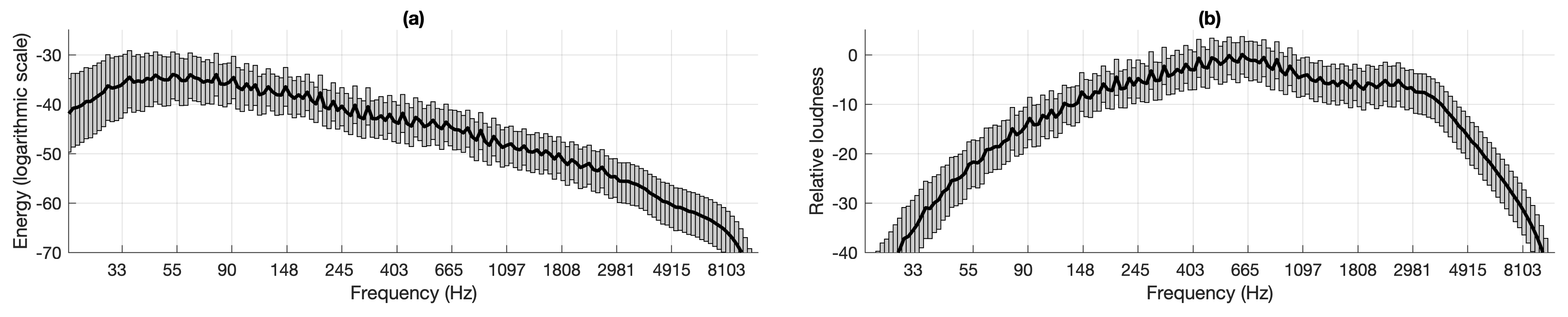
Figure 2: (a) power spectrum values for the BEA dataset. (b) relative loudness values.

Figure 2 (a) shows the power spectrum values for the BEA dataset. These results are consistent with those of Pestana et al., (2013). However, these power spectrum values are not an accurate reflection of what the listener actually hears. Humans are not equally sensitive to all frequencies (Fletcher and Munson,, 1933). Several models exist for the level of tones that are perceived as equally loud by human listeners depending on their frequency and sound pressure level. One such model is ISO226:2003 (ISO,, 2003). Figure 2 (b) shows the power spectrum weighted using the ISO226:2003 equal-loudness contour corresponding to 50 phon, which is the median contour. Most notably, bass frequencies become attenuated. To more accurately reflect what the listener hears, we weigh the audio using the ISO226:2003 50 phon equal-loudness contour and evaluate the above features on both raw and weighted audio (see section 10 for more details).

4 Results

4.1 Measures of HR-inharmonicity

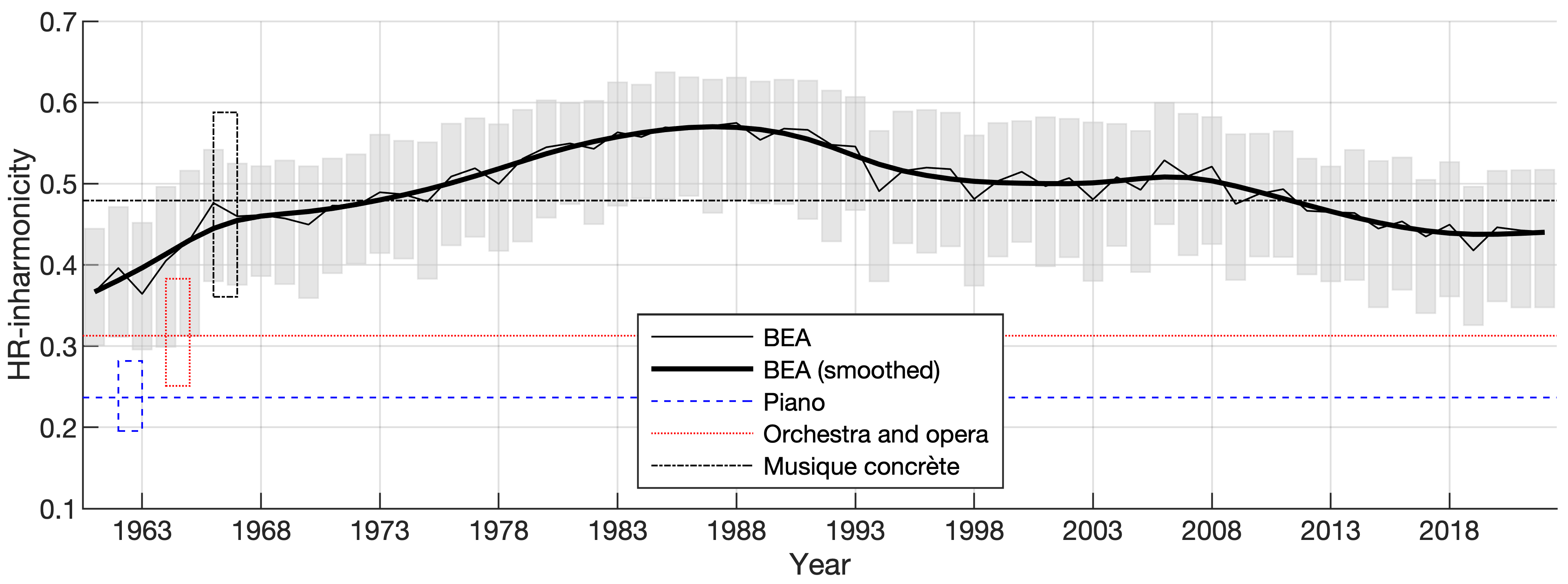
Figure 3: HR-inharmonicity for the four datasets. As in all the following similar figures, the lines represent median values, and the boxes represent interquartile ranges.

Figure 3 shows HR-inharmonicity for the four datasets. As autocorrelation is robust to level, the tracks are first gated to remove low-level parts (extensive for instance in bonus tracks), which would result in very low feature values as a result of the analysis of the background noise. The gating process only retains the parts of the original audio whose RMS power is above -20dB after peak normalisation. From Figure 3, it is possible to make the following observations.

1. HR-inharmonicity of popular music is comparable to that of musique concrète. Both are more HR-inharmonic than piano and orchestral music. It is noteworthy that the two music categories that heavily use production techniques in the recording studio have similar HR-inharmonicity values.

2. HR-inharmonicity of popular music is greater than that of orchestral music. Yet, orchestral music features a large number of instrumental sources, from typically 14–16 players during the second part of the 18^th century to 60–500 instrumentalists and voices during the 19^th century (Spitzer and Zaslaw,, 2001). It suggests that greater HR-inharmonicity (lower pitch strength) in popular music may derive from other causes than the number of sources, such as the presence of less ‘pure’ intervals and/or noise.

3. Popular music evolution over the years shows an increase in HR-inharmonicity (a decrease in pitch strength) until the mid-1980s, followed by an irregular, slower decrease that has continued up to the present day.

In section 6.5, we point out that HR-inharmonicity is correlated with the music’s ‘roughness’ (in the sense of Masina et al.,, 2022).

4.2 Measures of peak prominence

]

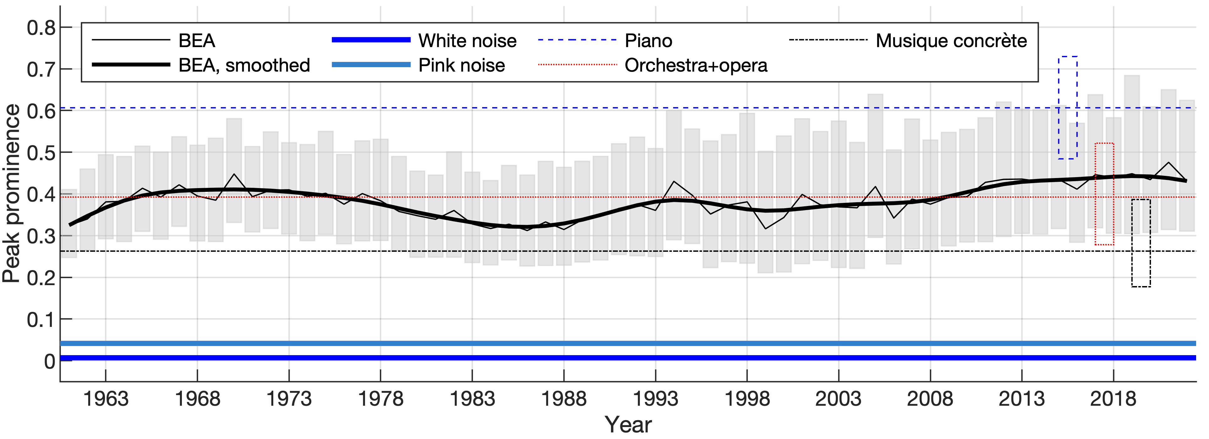
Figure 4: Measures of peak prominence for the four datasets, compared with values for pink noise and white noise.

Figure 4 shows peak prominence for the four datasets. From this graph, we can make the following observations.

1. The values corresponding to white noise and pink noise are similar. The peak prominence values for white noise and pink noise are close to each other and clearly separated from music. It shows that peak prominence is robust to the global spectral envelope of the signal (which is not the case for spectral flatness as mentioned above).

2. Popular music and orchestral music are similarly noisy. From Figure 3, we derived that greater inharmonicity in popular music may stem from the use of inharmonic sources, more inharmonic musical intervals, and/or noise. We can now exclude noise from the causes. The greater HR-inharmonicity observed in popular music is therefore likely to derive from a greater use of complex tones with inharmonic partials as well as more frequent use of inharmonic intervals between complex tones.

3. Piano music is less noisy than popular music, and musique concrète is noisier.

4. In the case of popular music, there is a local maximum at around 1970, a local minimum during the mid ’80s, and peak prominence increases slowly after 1986, continuing up to the present day. Notice that the peak prominence’s interquartile range generally increases over the entire period considered.

4.3 HR-inharmonicity and peak prominence: BEA dataset

Figure 5 (a) shows the result of the HR-inharmonicity vs. noisiness measures on the unweighted BEA dataset, including the evolution of both features according to the music’s year of release. For a single HR-inharmonicity value (same vertical position), it is possible to distinguish between inharmonicity that arises from noise (right-hand side of graph) or intervals between discrete components (left-hand side of graph). In Figure 5 (a), the bottom left corner of the graph corresponds to low noise and low HR-inharmonicity; whilst the top right corner corresponds to high noise and high HR-inharmonicity. The diagonal line extending from the bottom left of the graph to the top right corresponds to an increasing sum of noise and HR-inharmonicity. It is the axis that explains the most variance in the distribution.

Figure 5 (b) shows the result of the distribution’s PCA. In the upper two quadrants of the PCA graph, a relatively high proportion of the total amount of noise and inharmonicity is due to inharmonic intervals; while in the lower two quadrants, we have a relatively high proportion of the total amount of noise and inharmonicity being due to noise. Music tracks in the upper-right part of the PC1 vs. PC2 representation feature the highest amount of inharmonic relations between partials (high total amount of noise and inharmonicity, low proportion of this being due to noise). Conversely, tracks in the lower-left part feature the lowest density of inharmonic relations between partials.

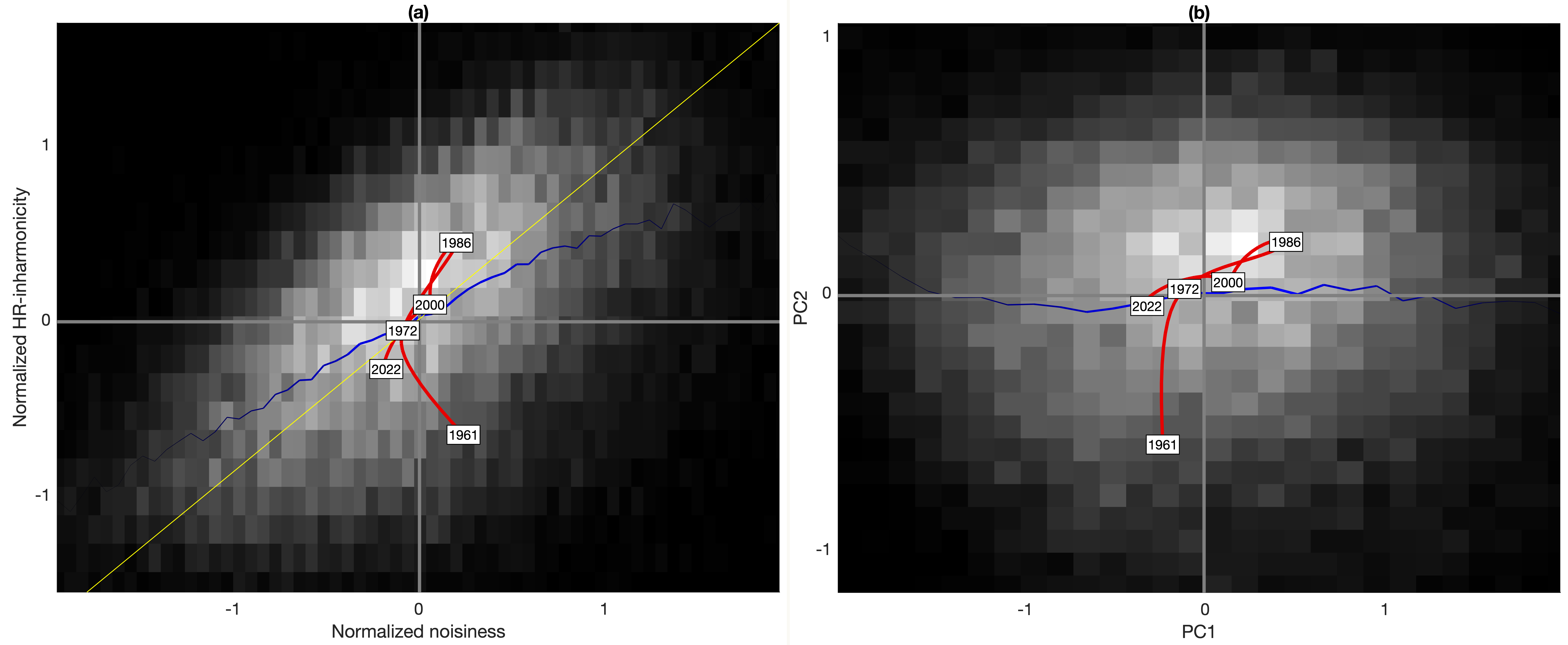
Figure 5: Noisiness and HR-inharmonicity in the BEA dataset. In (a), the $x$-axis is noisiness, while the $y$-axis is HR-inharmonicity. Distributions are made closer to normal by skewing ($x_{norm}=x^{0.18}$ and $y_{norm}=y^{0.21}$) and normalising (subtraction of the median and division by the interquartile range). The gray lines indicate the median values for each axis. The blue line indicates the median inharmonicity value for a given noisiness value. The yellow line shows the axis that explains the most variance in the distribution. The red curve shows how the centroid for the music in the dataset from a particular year evolves over the period 1961–2022, smoothed for readability purposes. The amount of smoothing is similar to that of the ‘smoothed’ BEA curves in Figures 3 and 4. (b) shows the results of carrying out a PCA on the results shown in the graph on the left, with $x$-axis being PC1 and $y$-axis being PC2. The blue line indicates the median PC2 value for a given PC1 value, and the red curve shows how the centroid for a particular year evolves over the period 1961–2022.

The graphs in Figure 5 suggest that the evolution of popular music between 1961 and 2022 can roughly be divided into three eras as follows.

1. 1961–1972    During this period, the evolution is parallel to the PC2 axis. The total amount of noise and HR-inharmonicity remains roughly constant but the relative amount of HR-inharmonicity increases, indicating that higher HR-inharmonicity values are due to an increase in the use of inharmonic intervals between partials rather than an increase in noise. It also indicates a decrease in the relative amount of noise. The end of the time frame corresponds to the advent of extensive multi-tracking (Milner,, 2011). We take it as a starting date for music referred to as ‘Contemporary Popular Music’ (CPM) in the sense of Deruty et al., (2022), with the use of extensive multi-tracking and, more generally, heavy use of the recording studio.

2. 1972–1986    During this period, there is generally increasing noise and increasing HR-inharmonicity with a relatively slightly greater increase in HR-inharmonicity, indicating that a slightly greater proportion of the HR-inharmonicity is due to inharmonic intervals, not noise, towards the end of this period.

3. 1986–2022    During this period, the trend of the previous period is reversed and extends even beyond the values at the end of the first period (i.e., the value for 1972). During the period 1986–2022 there was a general decrease in the total sum of noise and HR-inharmonicity, with music of today having, on average, roughly the same total amount of noise and HR-inharmonicity as music from the early 1960s. However, the amount of HR-inharmonicity has fallen more than the amount of noise, meaning that the proportion of HR-inharmonicity in the sum of HR-inharmonicity and noise (i.e., the PC2 value) has slightly fallen. In other words, the music of today has roughly the same total amount of noise and HR-inharmonicity as the music from the early 1960s, but a much higher proportion of this sum is due to HR-inharmonicity caused by inharmonic intervals rather than noise.

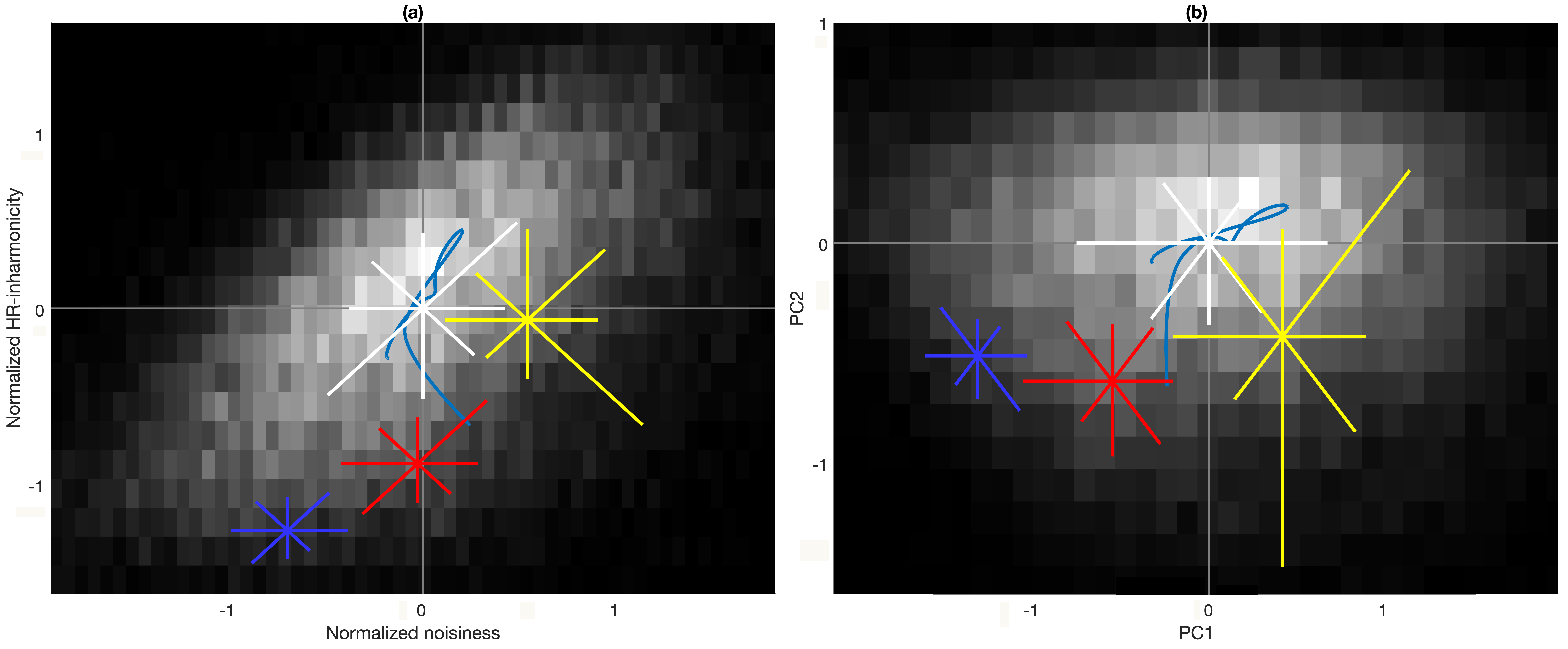
Figure 6: Respective positions of the four datasets. (a) HR-inharmonicity and noisiness. (b) PC1 and PC2 (as in Figure 5). The white, red, blue, and yellow stars respectively correspond to the BEA, orchestra, piano, and musique concrète datasets. The stars’ lines start at the median coordinates for each dataset, and stop where half of the points starting from the median were met.

4.4 HR-inharmonicity and peak prominence: all datasets

Figure 6 compiles the distribution values for the four datasets. As the distributions involving the four datasets are multimodal, we do not re-evaluate the PCs on the entire data, but keep the BEA’s PCs as axes. From Figure 6, we can observe the following:

1. Popular music from the beginning of the 1960s shows feature values that are not too different from that of orchestral music. However, CPM (popular music after 1972) uses more inharmonic intervals.

2. The ratio of HR-inharmonicity to noise is similar for piano music, orchestral music and musique concrète. However, the total amount of HR-inharmonicity and noise increases from piano music to orchestral music to musique concrète. The ratio of HR-inharmonicity to noise is higher for CPM than the other genres, indicating that relatively more of the HR-inharmonicity in CPM is due to inharmonic intervals.

3. As we will discuss in more detail below in section 5.3, Musique concrète and CPM use similar ‘resources of the performance’ (Parry,, 1911), that is to say, they are both typically created in music production studios using electronic technology. In McPherson and Tahıroğlu,’s (2020) terms, musique concrète explores a noisier ‘space for musical exploration’ with fewer inharmonic intervals between partials, and CPM explores a less noisy space with more inharmonic intervals. Both are equally distant from orchestral music.

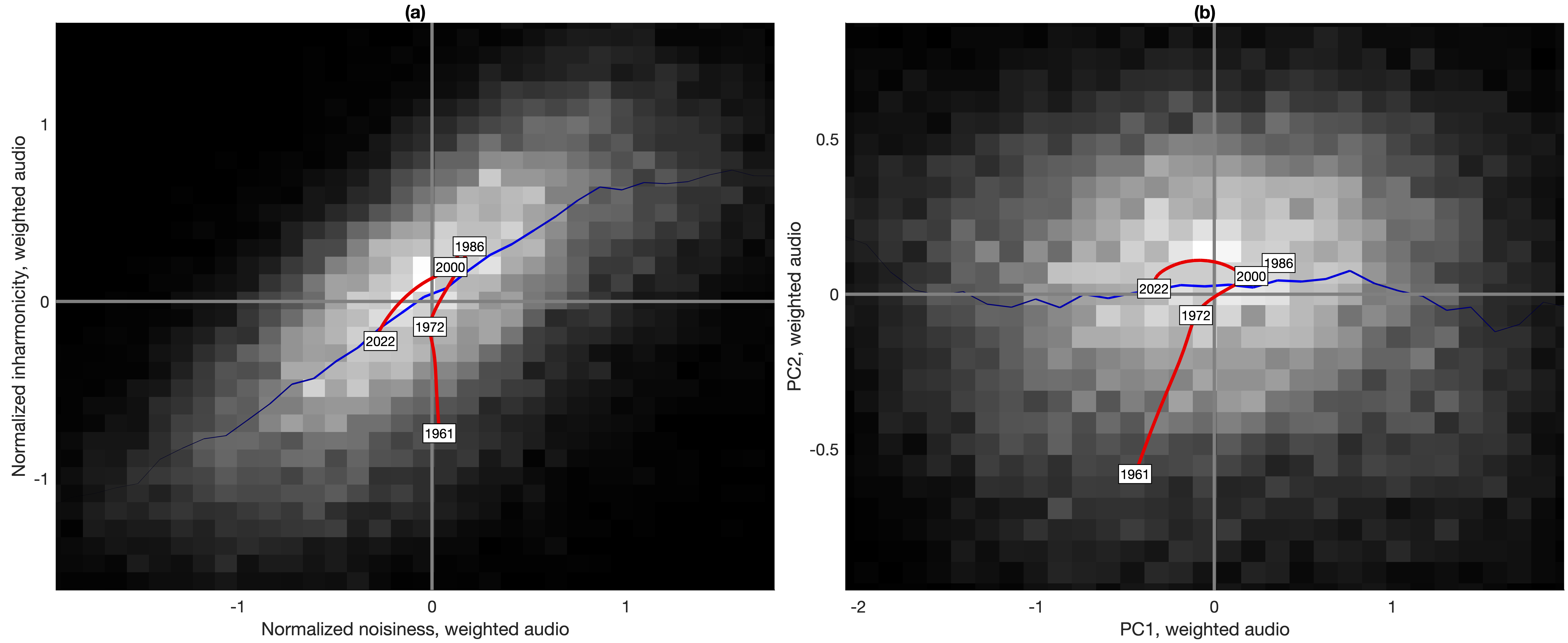
Figure 7: BEA dataset. (a) Normalised noisiness and inharmonicity from weighted audio. As in Figure 5, distributions are made closer to normal by skewing ($x_{norm}=x^{0.39}$ and $y_{norm}=y^{0.14}$) and normalising (subtraction of the median and division by the interquartile range). (b) PC1 and PC2 from weighted audio.

4.5 HR-inharmonicity and peak prominence, weighted audio

Figure 7 (a) shows the evolution of HR-inharmonicity and noisiness from weighted audio. Figure 7 (b) shows the evolution of PC1 and PC2 from weighted audio. Figure 7 may better reflect what is actually heard than Figure 5 (unweighted audio) while minimizing objective aspects of the signal that may be less perceptually salient, such as high energy values at the bottom end of the spectrum. The observable differences between Figures 5 and 7 may be summarised as follows.

1. The increase in the ratio of interval inharmonicity to noisiness (PC2) from 1961 to 1972 in Figure 5 is accompanied by a noticeable increase in total inharmonicity and noise (PC1) in Figure 7.

2. Between 1986 and 2000, the fall in inharmonicity to noise ratio (PC2) seems less than it does when viewed in terms of unweighted audio. It suggests that the faster evolution witnessed from non-weighted audio derives from very low frequencies. In other words, the faster evolution originates from a change in the properties of the medium in addition to that of the content. The weighting function gives relatively much less weight to the lower frequencies, meaning that the decrease in lower frequency energy between 1986 and 2000 would have less of an effect on the weighted audio graph of PC2.

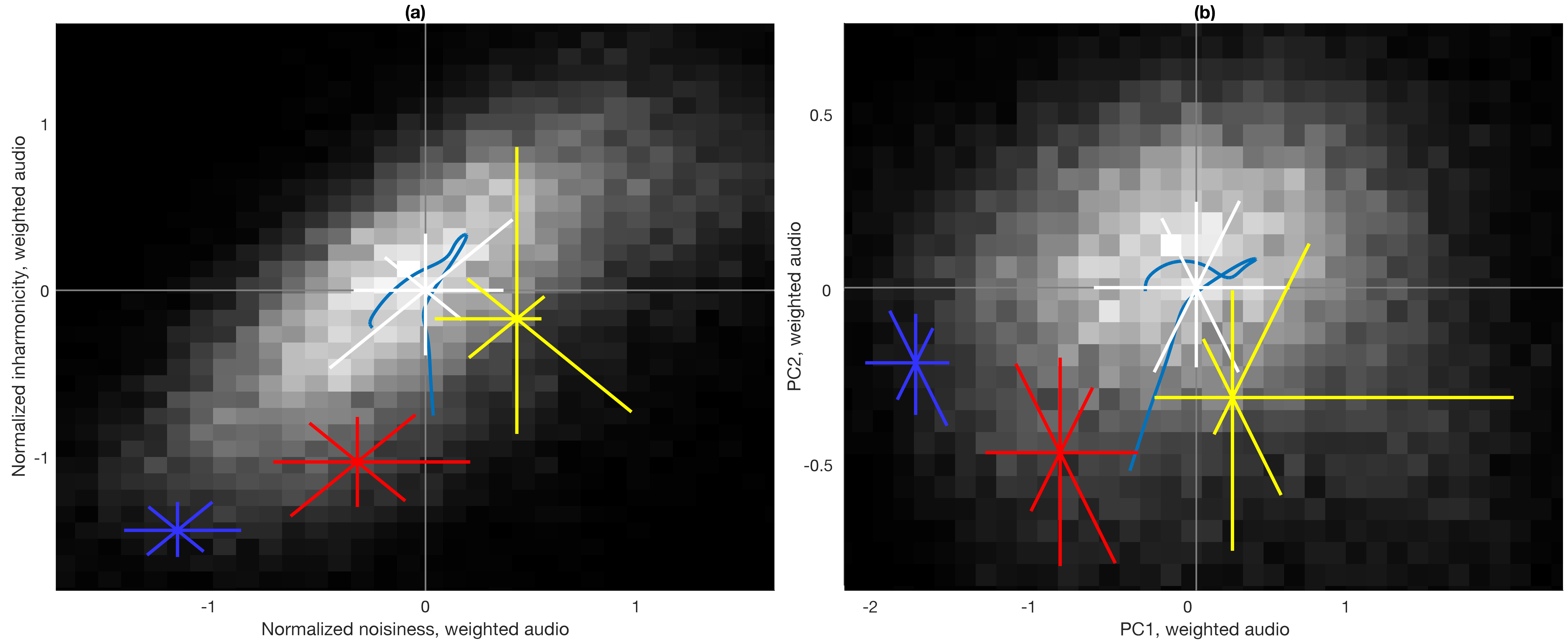
Figure 8: Respective positions of the four datasets using weighted audio. (a) Inharmonicity vs. noisiness; (b) PC2 vs. PC1. The white, red, blue and yellow stars correspond, respectively, to the BEA, orchestra, piano and musique concrète datasets, as in Figure 6.

This ends the core part of the article. The following sections elaborate on several elements from sections 3 and 4.

5 On the influence of technology on music

The example shown in section 2, Figure 1, features audio produced by a composite setup of digital instruments: superimposition of a Spectrasonics Omnisphere bass with a Eurorack setup involving FM synthesis, voltage-controlled amplifier, envelope, and ring modulator modules. It would have been difficult to produce using instruments based on the principle of the acoustic resonance. The present section elaborates on the relationship between technology and the resulting music. In section 5.1, we mention relations between the resources of the performance and the musical output. In section 5.2, we briefly focus on modern music production technology. In section 5.3, we explain the reasoning that brought us to study inharmonicity and noise in the first place. In particular, greater inharmonicity may be a case of CPM at least partially abandoning musical notes as a building block.

5.1 Resources of the performance and musical idioms

Music involves what Parry, (1911) calls the resources of the performance, such as the human voice and musical instruments. In Western classical music, a widespread class of such resources involves instruments based on acoustic resonators, of which examples are the vibrating string and the vibrating air column. Such acoustic resonators produce waveforms that feature a strongly periodic behaviour. The periodic part of such waveforms is usually modeled as the weighted sum of components based on a fundamental frequency and a series of overtones, whose frequencies are (close to) integer multiples of that fundamental (Young,, 1952).

According to Huron and Berec, (2009, p. 103), idiomaticism is, ‘of all the ways a given musical goal or effect may be achieved, the method employed by the composer/musician [that] is one of the least difficult’. Given an acoustic instrument that involves an acoustic resonator, it is easy to produce a harmonic or quasi-harmonic sound. Harmonic or quasi-harmonic sounds may therefore be described as idiomatic to instruments involving acoustic resonators.

The resulting sounds are used as elements of the musical discourse. In the case of acoustic resonators, the pitch impression derived from the harmonic or quasi-harmonic sound is denoted as a musical note, which is then used as a building block for writing musical phrases and chords. In Pascall,’s (2001) terminology, the idiom resides in the possibilities (for instance, the musical phrases and the chords) offered by the characteristic elements stemming from the use of the instrument. The properties of the sounds produced by acoustic resonators may also condition specific aspects of the musical discourse. For instance, the position of harmonics is an important factor in the determination of the musical temperament (Barbour,, 2004), and rules of Western counterpoint, such as the prohibition of parallel unisons, octaves, and fifths, can be linked to the properties of the waveform resulting from acoustic resonators (Huron,, 2001).

By providing a larger variety of resources, technological progress may influence musical idioms. In the 20^th century, one outcome of technological progress was signal analysis. Musicians such as Gérard Grisey took advantage of technology to produce spectral music, in which the score is derived from the positions of the harmonics of an acoustic instrument. One musical parameter becomes the deviation from the positions of the harmonics, resulting in a gradation from a harmonic texture to an inharmonic texture (Rose,, 1996). In this case, the idiom according to Huron and Berec, (2009) is the orchestral texture, and the idiom according to Pascall, (2001) is the gradation.

More generally, the 20^th and 21^st centuries brought considerable technical innovation in music technology (Webster,, 2002). Examples include non-acoustic musical instruments such as the Ondes Martenot (1928) (Orton,, 2001), the Moog analog synthesiser (1964) (Porcaro,, 2001) and digital synthesisers such as the FM-based Yamaha DX7 (1983) (Mattis,, 2001), which played a key role in popular music from the ’80s (Lavengood,, 2017, p. 36). Another key innovation resides in the practice of sound recording, which has been in a constant state of development since 1877 (Mumma et al.,, 2001). At least some technologies from the 20^th and 21^st centuries can be associated with musical idioms. For instance, continuously evolving frequencies can be identified as idiomatic (in the sense of Huron and Berec,, 2009) to the Ondes Martenot. Distortion can be identified as idiomatic to the use of analog circuitry, resulting in an idiom (still in the sense of Huron and Berec,) that is a definitive feature of musical genres such as heavy metal.

5.2 The ‘utopian vision of a boundless space for musical exploration’

The advent of specific idioms is not the only consequence of technological innovation. Music-related technology can assume various forms and is involved in various stages of the processes of producing music and engaging with it. One of these aspects is the compositional process itself. For instance, before the 16^th century, paper was expensive and erasable pencils did not exist (Charlton and Whitney,, 2001). As a result, composers did not have the opportunity to sketch and draft musical ideas (Bent,, 2001). The introduction of cheaper paper and erasable pencils modified the composition process. More recently, one consequence of technological progress in the composition process is the use of the recording studio for its own creative potential (Moylan,, 2014). Spicer, (2004) directly links ‘accumulative’ and ‘cumulative’ forms in pop-rock music to the rapid advances in recording technology.

During the 1990s, with the advent of the home studio, the practices that were previously exclusive to the professional studio became universally available. Almost anybody with a computer could now assume a musician–engineer hybrid role (Pras et al.,, 2013; Bell,, 2014) in a music production process to which ‘[t]he micro-manipulation of digital audio has become more and more the primary focus’ (Théberge,, 2001).

We have argued above that the recourse to musical notes can be considered as idiomatic to the use of acoustic resonators. In other words, instruments involving acoustic resonators favor the constraint (McPherson and Tahıroğlu,, 2020) according to which music should involve symbols referred to as ‘notes’, each of which denotes a harmonic or quasi-harmonic complex tone based on a particular fundamental frequency that remains approximately constant throughout the note’s duration. In the studio environment, this particular constraint disappears. One important issue becomes the determination of the idiom used by musicians in the absence of such a constraint. The issue relates to McPherson and Tahıroğlu,’s (2020) concern, according to which ‘even if we were to achieve the utopian vision of a boundless space for musical exploration, we would still be left with the question of what possibilities musicians would choose to explore within it’.

5.3 To what extent do idioms of popular music involve musical notes?

Musique concrète is an instance of music in which musicians have abandoned the musical note as a building block while working in the recording studio (Schaeffer,, 2020). This music genre, derived from Schaeffer,’s (1966) experiments, often does not involve elements that prompt a clear sensation of pitch. Still, musique concrète is not entirely devoid of pitch. According to Yost, (2009), ‘[m]usic without pitch would be drumbeats, speech without pitch processing would be whispers, and identifying sound sources without using pitch would be severely limited’. Such a description does not apply to musique concrète, as evidenced by pieces such as Temps de Pointe in Pierre Henry’s Mouvement-Rythme-Etude or Bernard Parmeggiani’s Ondes. Nevertheless, transcribing musique concrète to standard staff notation is generally difficult at best. Instead, transcriptions of musique concrète have been seen to involve freely drawn shapes that may reflect dynamics or timbre perception (Favreau et al.,, 2010).

From a commercial or large-scale social perspective, musique concrète might be considered a niche. The music charts indicate that the music that is most listened to is recent popular music. Popular music is a broad category that is distinguished from folk music and art music by its use of recorded sound as the main mode of transmission (Tagg,, 1982; Middleton,, 1990; Mazzanti,, 2019). It is characterized by commercial/industrial interests, entertainment, and strong ties to mass media (Frith,, 2004).

Deruty et al., (2022) use the term Contemporary Popular Music (CPM) to refer to popular music that is ‘contemporary’ in the sense of ‘current’ or ‘present-time’. CPM is known for its focus on technological innovation and cross-cultural and cross-genre influences (Mazzanti,, 2019; Frith,, 2004). Examples of CPM genres include post-rock, rap/hip-hop, electronica, and non-Western genres such as K-pop, J-pop, Bollywood, and reggaeton. Bertin-Mahieux et al., (2011) use the term contemporary popular music in relation to tracks released from 1922 onwards. Here, we use the term to refer to popular music released since the beginning of the 1970s. A milestone for the start of this period could be Sgt. Pepper’s Lonely Hearts Club Band, as the first release of The Beatles’ studio era (McCartney and Miles,, 1997). The dataset that we explore includes popular music released since 1961. Like musique concrète, recent popular music is produced in the recording studio. In Parry,’s (1911) terms, these two apparently very different categories there share the same ‘resources of the performance’ (the studio), and therefore have similar constraints and affordances.

Has popular music abandoned musical notes as its building blocks? Huang et al., (2020) distinguish several building blocks in the making of popular music, amongst which are melody, harmony, and percussion. The ‘melody’ and ‘harmony’ building blocks suggest that popular music can be at least partially transcribed to musical notes, either automatically (e.g., Bertin-Mahieux et al.,, 2011) or manually (e.g., Tagg,, 1982). The ‘percussion’ building block has been considered important enough to form the subject of research in both automatic transcription (Wu et al.,, 2018) and musicology (e.g., Mowitt,, 2002). From the perspective of physics, percussion instruments such as snare drums have been identified as featuring clear stochastic noise components (Fletcher and Rossing,, 2012, pp. 602-606). From the perspective of signal processing, percussive elements have been considered noisy impulses, forming ‘vertical ridges with a broadband frequency response’ (Fitzgerald,, 2010). Both perspectives suggest that the transcription of percussion to musical notes is, at best, difficult.

Percussion is not the only aspect of CPM that creates difficulties for meaningful transcription to musical notes. For instance, the practice of sampling has been documented to bring real-life noisy sounds into the music (Forman and Neal,, 2004, p. 408). The noise surrounding each partial in guitar distortion (Berger and Fales,, 2005, p. 184) may blur frequency values and therefore make pitch identification difficult. The fact that not all popular music can be meaningfully transcribed to notes (i.e., staff notation) raises the following question: is it possible to quantify the extent to which popular music deviates from being the result of a combination of ‘notes’? In other words, to what extent does it deviate from being produced (or producible) by some combination of acoustic resonators or technological devices that emulate acoustic resonators? We hope this article provides the beginning of an answer to this question.

6 A study of HarmonicRatio

In this section, we shall look more closely into the HarmonicRatio feature introduced in section 3.2.1. While it is not the focus of this paper to provide a complete understanding of the relations between the notions of ‘harmonicity’, ‘inharmonicity’, and the HarmonicRatio feature, we need an intuitive understanding of the feature’s behaviour, so that we can interpret the results of the subsequent measures involving HarmonicRatio.

6.1 Conventions

We use the following terminology:

1. The term partial denotes the spectral representation of a single periodic sine wave.

2. A harmonic complex tone designates an ensemble of partials that are integer multiples of a fundamental frequency.

3. An inharmonic complex tone designates a tone (i.e., it is perceived to have a pitch) that consists of an ensemble of partials that are near-integer multiples of a fundamental frequency. Fletcher et al., (1962) and Rasch and Plomp, (1982, p. 9) provide examples of such tones.

4. In a harmonic or inharmonic complex tone, an overtone can be any of the partials except the one that corresponds to the fundamental frequency.

5. A harmonic is any sinusoidal component of a harmonic complex tone, with the $n$th harmonic having a frequency that is $n$ times the frequency of the fundamental (so the fundamental is the first harmonic).

In this section, harmonic complex tones are generated using the model mentioned in Mauch and Dixon, (2010) and previously introduced by Gómez, (2006), according to which the $k$^th partial, denoted by $a(k)$, is assigned an amplitude $s^{k-1}$ for some constant $s<1$. Unless stated otherwise, we use 10 harmonics over a 220Hz fundamental (A3) and set $s=0.8$.

6.2 One complex tone

We start with the case of a single isolated complex tone. Figure 9 shows the evolution of HarmonicRatio values in four cases as follows.

1. Increasing number of inharmonic partials in an initially harmonic tone.

2. Increasing number of inharmonic partials in an initially harmonic tone, with harmonics having less energy than in case 1 ($s=0.7$).

3. Frequency shifting of one single partial (arbitrarily, partial 4) of an initially harmonic tone.

4. Superposition of two sine waves of equal power. The frequency of the first sine wave is 220Hz. The frequency of the second sine wave ranges from 220Hz to 880Hz.

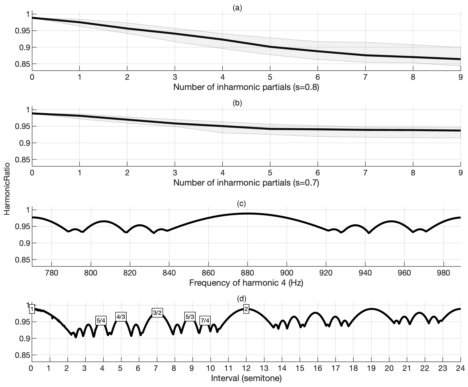
Figure 9: (a) HarmonicRatio resulting from an increasing number of inharmonic partials in an initially harmonic complex tone ($f0=200$Hz, 10 harmonics). The inharmonicity of the partials is random, the representation summarises observations from 50 tones, the black line denotes the median over the 50 observations, and the gray area the 25^th and 75^th percentiles. (b) Same as top graph, but with harmonics of lower energy. (c) HarmonicRatio resulting from the frequency shift of a single partial. (d) HarmonicRatio resulting from the superposition of two sine waves depending on the interval between them. The text boxes show the frequency ratios of the ‘purer’ intervals inside the first octave. The $y$-axis scale is identical for all graphs in order to facilitate comparison.

The results are shown in the four graphs in Figure 9, from which we can derive the following observations:

1. Figure 9 (a) confirms the MPEG-7 specification’s interpretation (ISO,, 2001), in the sense that an increasing proportion of inharmonic components in an initially harmonic complex tone indeed decreases the HarmonicRatio value.

2. Figure 9 (b) shows that the resulting HarmonicRatio value depends on the energy of the inharmonic components. As the inharmonic components become relatively more intense, the HarmonicRatio value falls.

3. Figure 9 (c) shows that when one single partial is inharmonic, the resulting HarmonicRatio value depends on the partial’s frequency.

4. Figure 9 (d) elaborates on the influence of the intervals between two partials on the resulting HarmonicRatio values. (i) ‘Purer’ or ‘simpler’ intervals, i.e., intervals that can be expressed as a fraction composed of smaller integers (Vos and van Vianen,, 1985), are local maxima of the HarmonicRatio values. The ratio’s denominator is a key influence on the HarmonicRatio of the interval. (ii) Intervals result in comparatively higher HarmonicRatio values as they get wider. Observations (i) and (ii) are reminiscent of sensory dissonance (Sethares,, 2005, p.46, p.85), and what Masina et al., (2022) refer to as ‘roughness’, following Hutchinson and Knopoff, (1978) and Plomp and Levelt, (1965).

To summarise, given one complex tone, low HarmonicRatio values may be the combined result of the following:

1. a high proportion of intervals between partials that are not close to ‘pure’ intervals; and

2. the intervals that are far from ‘pure’ intervals involve partials with high energy values.

6.3 Several complex tones

The properties leading to low HarmonicRatio values in single complex tones remain valid in the case of the superposition of several complex tones. One difference lies in the fact that the distribution of the complex tones’ fundamentals often reflects scales or tuning systems (e.g., a diatonic scale or 12-tone equal temperament). We examine the HarmonicRatio values resulting from the superposition of complex tones whose fundamentals conform to different scales. We start from one harmonic complex tone, and add complex tones whose fundamentals range from 220Hz to 2200Hz. We compare the HarmonicRatio measures in four cases:

1. the fundamental frequencies can take on any value;

2. their values are restricted to a chromatic scale using equal temperament;

3. their values are restricted to major triads using equal temperament; and

4. their values are restricted to major triads using the pure intervals shown in Figure 9.

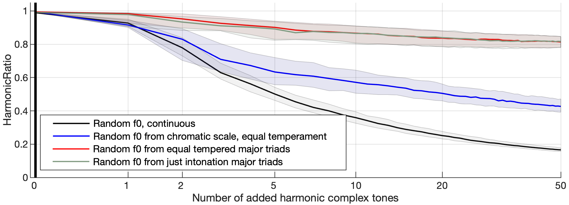
Figure 10: HarmonicRatio resulting from the sum of harmonic complex tones, depending on the distribution of fundamental frequencies. As the fundamental frequencies are randomly sampled from their respective distribution, the measures are performed 500 times. The solid lines represent the median, and the areas are bounded by the 25^th and 75^th percentiles.

The results are shown in Figure 10, from which we can observe the following:

1. A higher number of harmonic tones leads to decreasing HarmonicRatio values. In other words, the more voices in the music, the more it becomes inharmonic.

2. HarmonicRatio values are influenced by the scales on which the music relies. HarmonicRatio is lowest when the scale is continuous (case 1). It increases when the scale is restricted to the twelve-tone chromatic scale (case 2). It increases again when the fundamentals only constitute major triads (case 3). Finally, it remains similar when the major triads use pure intervals instead of equal-tempered intervals (case 4).

3. The very low HarmonicRatio values resulting from fundamental frequencies not following a discrete scale suggest that the presence of continuous frequency contours (e.g., human voices in music) may be a factor that lowers HarmonicRatio values.

Additionally, two factors that can influence HarmonicRatio values in the case of several complex tones derive from observations that were made in section 6.2 in the case of one single complex tone:

1. Proximity of f0s. We saw that closer partials generally result in lower HarmonicRatio values. As a result, fundamental frequencies that are close to each other (as may happen, for instance, in near-coincident musical voices) will result in relatively low HarmonicRatio values.

2. Voices of equal energies. In the case where all partials are inharmonic, e.g. in piano sounds (Fletcher et al.,, 1962), the lowest HarmonicRatio values will be obtained when the partials have approximately equal energy. This may happen with two musical voices of close energy. If the fundamentals are close in frequency, then the lowest HarmonicRatio values will be obtained if the fundamentals have the same energy.

To summarise, given several complex tones, low HarmonicRatio values may be the combined result of

1. a high number of simultaneous voices;

2. voices being close together in frequency;

3. voices having the same level;

4. musical intervals not being ‘pure’; and

5. a continuous distribution of f0 values.

6.4 Respective contribution of fundamental and overtones

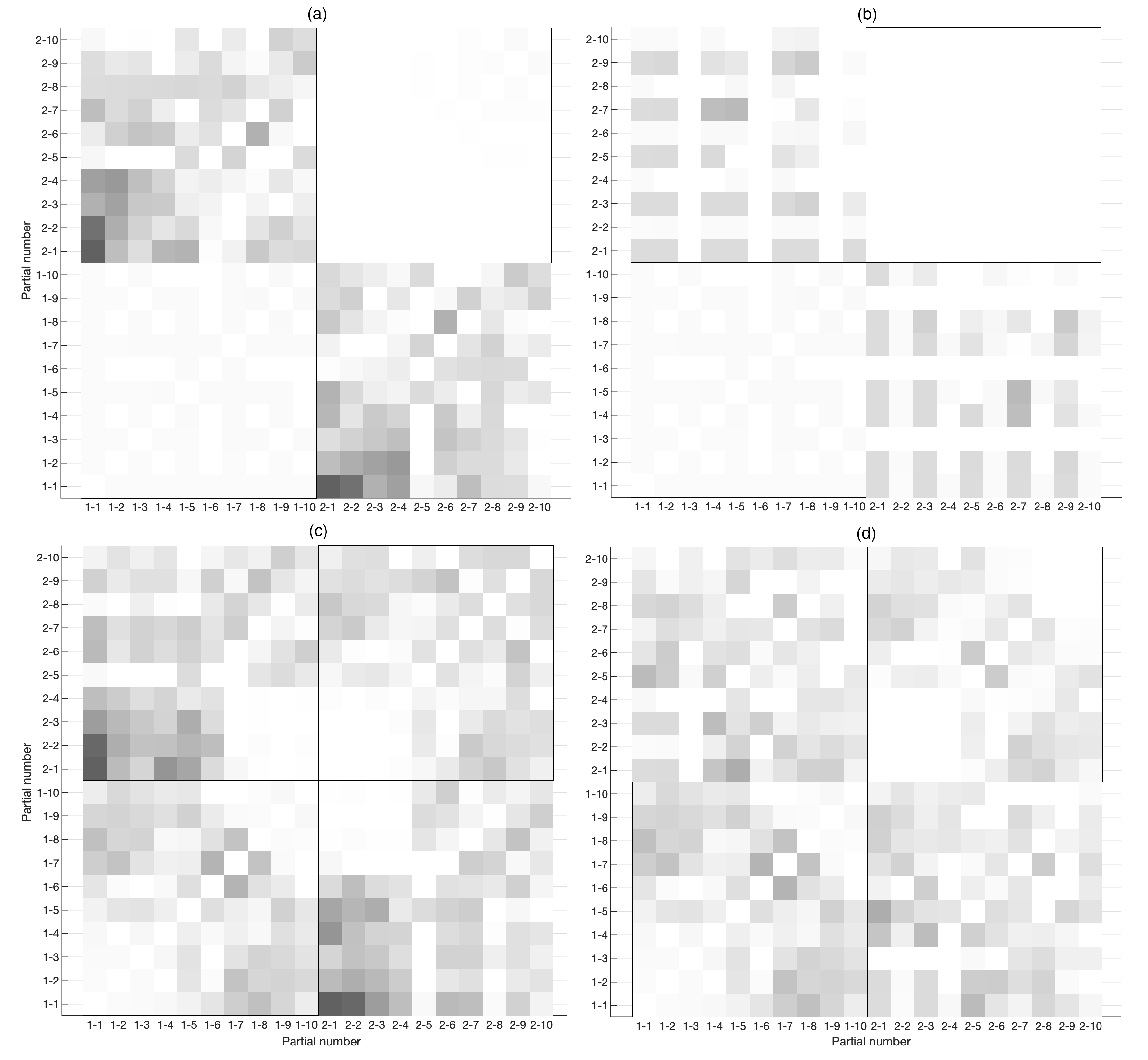
Figure 11: First row, HarmonicRatio derived from the pairwise combination of elements in two harmonic tones. Clearer shades correspond to higher values, and darker shades to lower values. The interval between the two tones is (a) 3 half-tones and (b) 5 half-tones. Partial numbers are written as ‘tone number-partial number’ (e.g., ‘2-3’ corresponds to the third partial of the second tone). Second row, (c) and (d), HarmonicRatio derived from the pairwise combination of elements in two inharmonic tones (same fundamentals as first row, inharmonicity coefficient is 0.002 as defined by Fletcher et al., (1962)).

Figure 11, graphs (a) and (b) show the HarmonicRatio values resulting from the pairwise superposition of each component of two harmonic complex tones. The tones leading to Figure 11 (a) and (c) have fundamentals that are 3 semitones apart (an equal-tempered minor third). The tones leading to Figure 11 (b) and (d) have fundamentals that are 5 semitones apart (an equal-tempered perfect fourth).

As shown in Figure 9 (d) in the case of two sine waves, the equal-tempered minor third corresponds to a lower HarmonicRatio than the perfect fourth. In the case of complex tones, we can make a distinction between harmonic and inharmonic complex tones:

1. Two harmonic complex tones (the two top graphs in Fig. 11)    For both the minor third and the perfect fourth, HarmonicRatio values deriving from the superposition of overtones inside one harmonic complex tone are higher than HarmonicRatio deriving from the superposition of overtones belonging to different harmonic complex tones. The observation would be valid for all intervals except the octave, in which case all the harmonics of the upper tone would coincide with harmonics of the lower tone and the HarmonicRatio values resulting from the interaction between harmonics within one of the complex tones would be no different from those resulting from the interaction between harmonics in different tones.

2. Two inharmonic complex tones (the two bottom graphs in Fig. 11)    HarmonicRatio values resulting from the superposition of partials within a complex tone are generally lower than in the case of harmonic complex tones. In the case of the five-semitone interval (right-hand side of figure), they are lower than the values resulting from the superposition of the fundamentals. The observation would be valid for all intervals corresponding to a high HarmonicRatio value.

To summarise:

1. Low HarmonicRatio values may originate from both the intervals between complex tones and the inharmonicity of individual complex tones.

2. Increasing the inharmonicity of individual complex tones reduces the relative influence on inharmonicity of the intervals between complex tones.

6.5 HarmonicRatio and acoustic beating

As mentioned in section 6.2, the behaviour shown by the graph at the bottom of Figure 9 is reminiscent of that of ‘roughness’. According to Masina et al., (2022), relations between the sensation of ‘roughness’ and acoustic beats were introduced in 1832–1837 by Foderà (Barbieri,, 2002) and in the middle of the 19^th century by Helmholtz (Helmholtz and Ellis,, 1885, pp. 197-211). Rasch and Plomp, (1982, p. 15) illustrate how acoustic beating corresponds to the sensation of ‘roughness’ when the interval between two tones is smaller than that of a critical band. We compare measures of acoustic beating and HarmonicRatio values deriving from the superposition of harmonic complex tones.

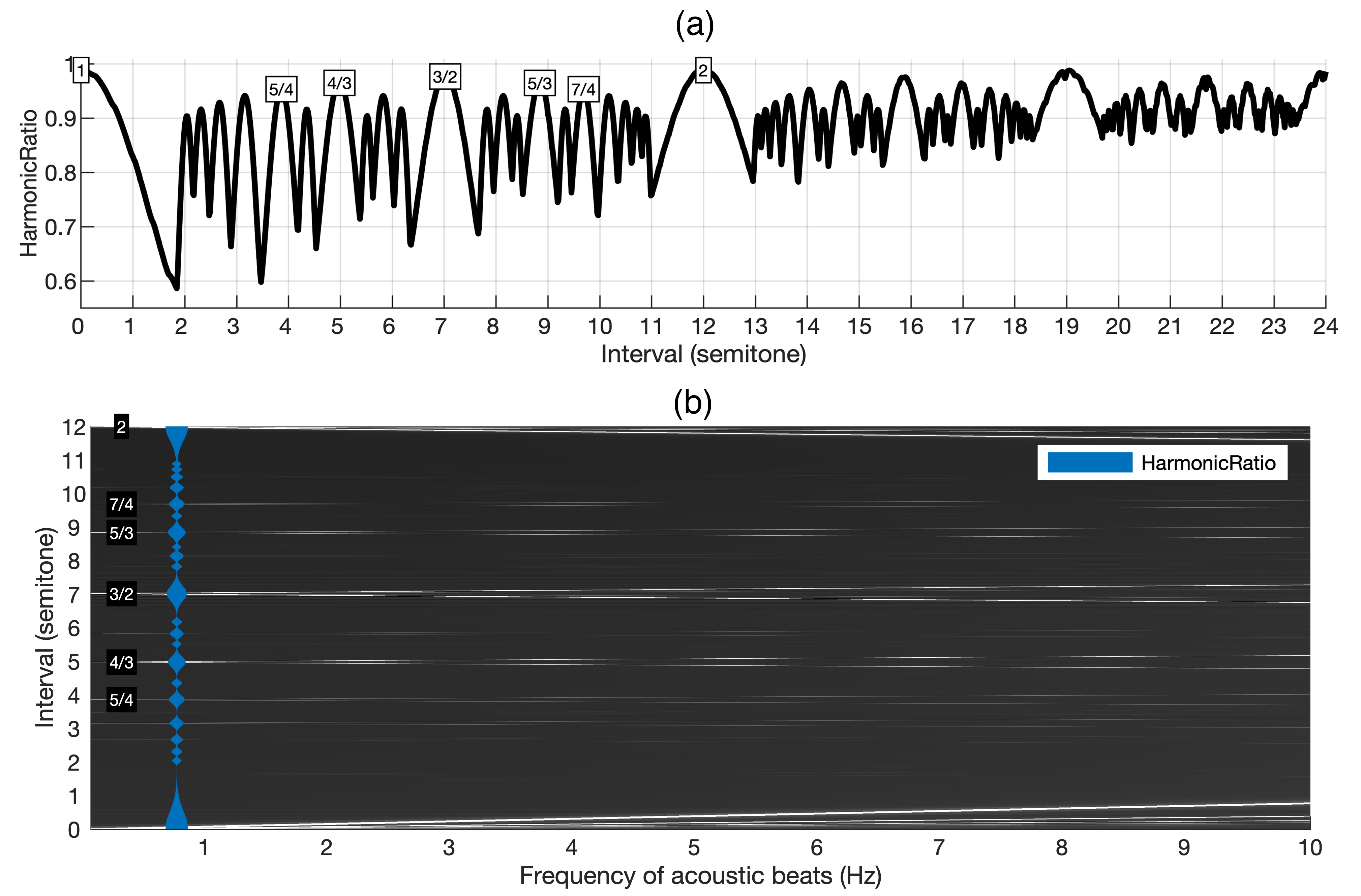
Figure 12: (a) HarmonicRatio resulting from the superposition of two harmonic complex tones depending on the interval between them (10 harmonics, $s=0.8$) As in Figure 9, bottom, the text boxes show the frequency ratios of the ‘purer’ intervals inside the first octave. (b) Frequency beating resulting from the superposition of two harmonic complex tones. The $y$-axis corresponds to the first part of the top graph’s $x$-axis. The $x$-axis is the frequency of the signal’s RMS. White values indicate a high RMS variation, in other words, a high acoustic beating amplitude. The width of the superposed blue area denotes the HarmonicRatio values as shown in the top graph. The location of the blue area along the $x$-axis is arbitrary.

Figure 12 (a) is the result of the same process as Figure 9 (d) using two harmonic complex tones instead of two sine waves. The f0 of the first complex tone is 220Hz and the f0 of the second complex tone ranges from 220Hz to 880Hz. In Figure 12 (b), we superpose the HarmonicRatio values from Figure 12, top, with measures of acoustic beating (background image). We evaluate acoustic beating by computing the power spectrum of the envelope (0.05s windows) of the sum of the two complex tones. High power spectrum values correspond to the presence of acoustic beating at the corresponding frequency. We use a higher number of harmonics (40) and a higher $s$ factor (0.95) so that the white lines deriving from acoustic beating are more visible. From these results, we can make the following observations:

1. Pure intervals correspond to infinitely slow acoustic beating (i.e., no beating). Increased deviation from pure intervals corresponds to acoustic beating becoming faster. In that sense, more ‘roughness’ may correspond to faster acoustic beats.

2. The local maxima of the HarmonicRatio values occur when acoustic beating is slowest. In that sense, high HarmonicRatio values is associated with low ‘roughness’ and slow acoustic beating.

From this point of view, results involving HarmonicRatio (such as in section 4) may equally apply to the period of the acoustic beating, in other words, the ‘roughness’ or acoustical ‘grit’ of the music.

6.6 HarmonicRatio and noise

The tones used to produce the results shown in Figures 9–12 were each composed of a finite number of sinusoidal components. Such signals do not contain noise. As previously mentioned in reference to Schneider and Frieler, (2009), inharmonicity can also stem from noise. In this case, low HarmonicRatio values can be understood in principle as being the result of the presence of inharmonic relations between the (infinite set of notional) sine waves that constitute the noise whose frequencies can be infinitesimally different from each other.

From the perspective of discrete spectral transforms, an infinite-length signal can be identified as devoid of noise when spectral bins with non-zero values are separated by bins with zero values. Conversely, the presence of noise may be characterised by several contiguous bins with non-zero values. In practice, however, it is difficult to define precisely what constitutes ‘noise’ in a spectral transform because

1. even the spectra of harmonic tones are not actually line spectra because they do not have infinite duration; and

2. a transform takes place on an audio window that covers a time span so that a sine wave with even small frequency changes within the window (such as the result of a vibrato) will not result in a line but in a distribution of frequencies.

As it is difficult to distinguish noise from spectral lines in practice, we choose not to distinguish between them. We fall back on the objective information we have. Thus, from a spectral domain perspective, the signal’s information is represented as values attached to spectral bins. Frequency intervals are only defined between the spectral bin center frequencies, and any information we derive from the signal originates from the values attached to the spectral bins. From this point of view, a feature representing the ‘degree of inharmonicity’ in the signal may be conceptualised as deriving from the ensemble of pairwise combinations between all frequency bins (positions and energy values). As a result, a feature representing the ‘degree of inharmonicity’ in the signal will not be able to distinguish between ‘inharmonic sounds which have little if any relevance for music (e.g., white or pink noise)’ (Schneider and Frieler,, 2009) and ‘coherent’ inharmonic signals, which ‘sound as stable and smooth as harmonic signals’ (de Boer,, 1956), i.e., inharmonic complex tones with a finite number of sinusoidal components. In light of the relation between HarmonicRatio and pitch strength mentioned at the beginning of section 3.2.1, the ‘first peak of the auto-correlation function’ (Patterson et al.,, 1996; Yost,, 1996, 1997; Shofner and Selas,, 2002) is unable to determine whether a lower pitch strength perception derives from relations between partials, or from noise. We need to find a method to estimate the relative extent to which inharmonicity results from the interaction between (approximately) discrete partials as opposed to the presence of noise.

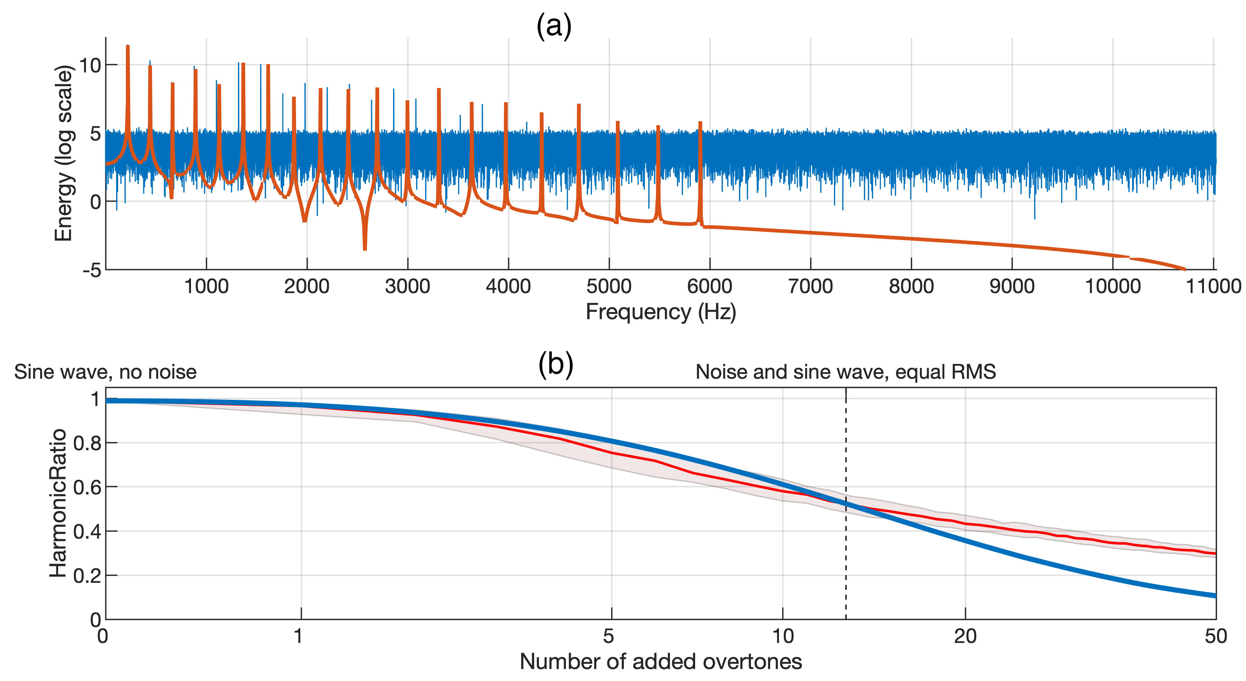
Figure 13: HarmonicRatio, inharmonicity and noisy signals. (a) The signals corresponding to the two spectra have the same HarmonicRatio value of 0.9558. The red signal is inharmonic, with an inharmonicity coefficient of 0.002 according to Fletcher et al., (1962). The blue signal is the sum of a harmonic complex tone and white noise. The white noise’s RMS power is 13.5dB below the harmonic tone’s. (b) Comparative decrease of HarmonicRatio values starting from a sine wave. The blue curve is the result of added white noise. The red curve is the result of adding sine waves of random frequencies. The frequencies being random, the experiment is repeated 200 times. The red area shows the 25^th and 75^th percentiles of the results.

Figure 13 (a) illustrates how an inharmonic complex tone and a harmonic complex tone with white noise can result in the same HarmonicRatio value. Conversely, given a HarmonicRatio value less than 1, the original audio may consist of a non-inharmonic tone superposed with noise, or of a noiseless inharmonic complex tone.

Figure 13 (b) illustrates how a sum of sine waves and a sine wave with white noise can result in the same HarmonicRatio values. Specifically, in this graph it can be seen that a sine wave superposed with noise of equal RMS power is as inharmonic on average as a sum of 14 sine waves of the same energy and random frequencies.

6.7 Inharmonicity as 1$-$HarmonicRatio.

The output of the HarmonicRatio feature can be viewed as a reflection of the pairwise relations between the values in all spectral bins, regardless of whether the spectral bin values originate from noise or from partials. High HarmonicRatio values correspond to harmonic partials without noise. Any deviation will lower the resulting HarmonicRatio values. The deviation can derive from inharmonicity in complex tones, inharmonic relations that derive from certain combinations of complex tones, and inharmonic relations deriving from the presence of contiguous non-zero spectral bins, which can originate from noise. This summary characterises an ‘inharmonicity’ feature, which we call ‘HR-inharmonicity’ and directly derive from HarmonicRatio:

$$\mathit{HR\mbox{-}inharmonicity}=1-\mathit{HarmonicRatio}\,.$$

7 ‘Noisiness’, spectral flatness and peak prominence

In the previous section, we established that:

1. A harmonic complex tone with noise and a noiseless inharmonic complex tone may lead to the same value of HarmonicRatio.

2. A discrete ensemble of sine waves with no harmonic relations and white noise added to a sine wave may lead to the same value of HarmonicRatio.

In order to discriminate between noiseless and noisy signals leading to the same value of HarmonicRatio, we need a feature that measures the noisiness of the signal. To that end, we introduce a new metric derived from the spectral flatness (Peeters,, 2004) and AudioSpectrumFlatnessType (ISO,, 2001) features, which is robust to the overall spectral profile.

Peeters, (2004, p. 20) defines spectral flatness as ‘a measure of the noisiness […] / sinusoidality of a spectrum’. It is computed using the ratio of the geometric mean to the arithmetic mean, which is equivalent to the Wiener entropy (WE) of the energy spectrum value. A comparison between the WE and the variance of the power spectra derived from the BEA dataset shows that the two measures are highly correlated (Pearson correlation = 0.9973). As a result, in the context of this study, it is possible to intuitively understand spectral flatness as similar to the variance of the power spectrum. Intuitively, low spectral flatness values (i.e., high WE and high variance) denote the presence of spectral peaks, while high values (i.e., low WE and low variance, ‘flat’ spectrum) denote a noise-like signal.

Spectral flatness is included in the Essentia toolbox (Bogdanov et al.,, 2013) as FlatnessDB and in the MPEG-7 standard as AudioSpectrumFlatnessType (ISO,, 2001, p. 26). For the evaluation of the spectrum, the MPEG-7 documentation specifies a logarithmic frequency resolution of a 1/4 octave. We prefer to use a higher resolution so that the spectral peaks are more clearly defined. We use one-quarter of a semi-tone (25 cents). This interval is close to a Pythagorean comma and of roughly the same order of magnitude as the minimum perceivable pitch difference (Zarate et al.,, 2012) or ‘just noticeable difference’ (Stern and Johnson,, 2010) for pitch. The use of such a higher resolution is made possible by the analysis taking place on the Fourier transform instead of the short-term Fourier transform as is the case in the MPEG-7 standard.

As a preliminary step, we calculate spectral flatness for the music datasets, for pink noise, and for white noise. The output value is $0.998$ for white noise. The value for pink noise ($0.84$) is between the values for the BEA dataset ($0.83$) and the orchestra dataset ($0.86$). The difference between the values for white noise and pink noise stems from the fact that the original spectrum is evaluated on a logarithmic frequency scale. In the case of white noise, bands are of constant width in terms of frequency; whereas, in the case of pink noise, they are decreasing. When we use a linear frequency scale, the situation is reversed. Spectral flatness is sensitive to the global envelope of the spectrum. The fact that the spectral flatness values of pink noise and music are similar, defeats the original purpose of measuring noisiness. We want to measure the prominence of the peaks, in other words, the noisiness of the signal, independently of the global envelope. Therefore, we perform median filtering on the spectrum before evaluating its WE. The filtering involves 8-bin windows (1 tone). Experiments show that window widths between 4 and 16 bins lead to comparable results.

When using median filtering, the values corresponding to the spectral troughs may be close to zero, with both positive and negative values. This poses a challenge when evaluating WE, which uses a geometric mean numerator and cannot be evaluated when negative values are present. One solution is to zero all negative values, but this will always result in WE being zero, as illustrated by Peeters, (2004, p. 20). To avoid this, we scale the filtered spectrum so that its minimum value is one. However, this process makes WE sensitive to gain, meaning that two identical audio samples with different levels will have different WE values. To address this problem, we first normalise the audio samples using RMS power to make the measure robust to gain. Finally, to make the distribution more normal and following the recommendations of Peeters, (2004, p. 20) in regards to what he calls ‘tonality measure’, we express the result on a log scale. We refer to the resulting feature as ‘peak prominence’.

To summarise, the steps leading to the measure of peak prominence are: RMS normalisation, power spectrum evaluation (log frequency scale, 25-cent wide bands), median filtering (8-bin windows), Wiener Entropy, and log of the result:

$$\mathit{Peak\>prominence}=\log(\mathit{WE}(\mathit{median\mbox{-}filtered\>spectrum\>of\>RMS\mbox{-}normalised\>audio}))\,.$$

Peak prominence was designed to be the opposite of ‘noisiness’, which leads to:

$$\mathit{Noisiness}=-\mathit{peak\>prominence}\,.$$

8 Influence of the medium and remastering processes

The medium on which the music is recorded may bring noise. According to Brandt et al., (2019), early recording media, such as wax cylinders, had signal-to-noise ratios (SNRs) of below 40 dB. Vinyl discs have SNRs of 55 to 60 dB, and magnetic tape storage SNRs of 60 to 70dB. To evaluate the influence of the noise brought by the medium on noisiness, we compute the difference between the noisiness in the original BEA files and the same files on which we add white noise corresponding to an SNR of 40dB. The median of the absolute value of the difference is 0.000007. In section 4.2, figure 4, typical noisiness values for the BEA dataset are shown to be ca. 0.3. The comparison suggests that the influence of the noise brought by the medium is negligible.

Music albums may be remastered. Deruty, (2011) suggests that remastering significantly affects the album’s loudness. We compared HR-inharmonicity values for the songs from the original and remastered version of the British band The Cure, as Deruty, (2011) did for loudness values. The median of the absolute value of the difference is 0.015 for non-weighted audio and 0.008 for weighted audio. In section 4.1, Figure 3, typical HR-inharmonicity values for the BEA dataset range between 0.3 and 0.63. Along with the influence of the background noise, the comparison suggests that the study’s results are robust to remastering processes.

9 Relations with some other diachronic studies

Mauch et al., (2015) investigate the US Billboard Hot 100 between 1960 and 2010. Using music information retrieval and text-mining tools, they demonstrate quantitative trends in their harmonic and timbral properties. Using NNLS Chromas (Mauch and Dixon,, 2010) and MFCCs, they find that ‘1964, 1983 and 1991 are periods of particularly rapid musical change’. They remark that ‘other measures may give different results’, which is indeed the case in this study, where we observe the fastest changes occurring throughout the 1960s (see Figures 5 and 7). The features used in Mauch et al., (2015) do not seem well-correlated to the features we use, suggesting that chromas and MFCC may fail to recognise certain properties of the music. As a general rule, it may be that the interpretation of feature-based studies should be limited to the interpretation of the features themselves rather than to ‘the music’ as a whole.

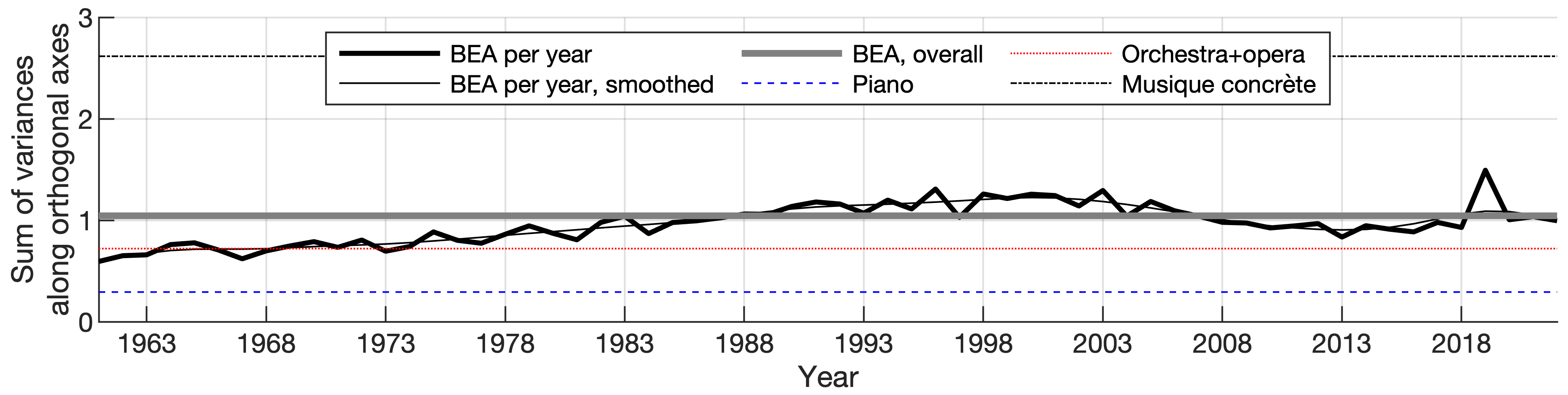
Figure 14: Variance of the distribution along PC1 and PC2 (unweighted audio).

In section 4.3, Figure 5, PC1 and PC2 are orthogonal. Therefore, the variance for the 2D data can be estimated as the sum of the variances along each axis. Figure 14 represents the sum of the variances along PC1 and PC2 for each dataset, as well as for the year-by-year data of the BEA dataset. The results are identical in terms of comparison for the original and PC representations. The following points are worth noting.

1. The variety of popular music in terms of the features we use is higher than that of orchestral music after 1978, and higher overall. It suggests that in terms of noise and HR-inharmonicity, popular music uses a wider ‘space for musical exploration’ than orchestral music.

2. The variety of musique concrète in terms of the features we use is greater than that of popular music. In terms of noise and HR-inharmonicity, Musique concrète takes greater advantage of the lack of constraints in the production process.

3. Serrà et al., (2012) find that the evolution of popular music goes ‘towards a consistent homogenization of the timbral palette’. Figure 14 suggests that no such homogenization of the timbral palette has taken place in terms of noisiness and inharmonicity (or, equivalently, peak prominence and pitch strength).

10 ELC weighting

This section elaborates on the difference between analyses performed using raw and weighted audio that was introduced in section 3.2.4.

Figure 15 (a) shows the power spectrum values for the BEA dataset according to the year of release. Figure 15 (b) shows the same values, normalised using each band’s mean. The lower graph clearly shows an increase in the power in the lowest two bands over the period. A similar evolution in the levels of bass is documented by Hove et al., (2019). Over the period represented by the BEA dataset, the lowest frequencies have become increasingly available for manipulation and processing due to technological progress in the recording process (Fine,, 2008). Note that there is a local maximum of energy above 2275Hz around 1986. The energy of harmonics around this time is closer to the energy of the fundamental. As seen in sections 6.2 and 6.3, louder inharmonic partials result in lower HarmonicRatio values. The local maximum of energy above 2275Hz around 1986 may, therefore, be a contributing factor to the local maximum of HR-inharmonicity around that time.

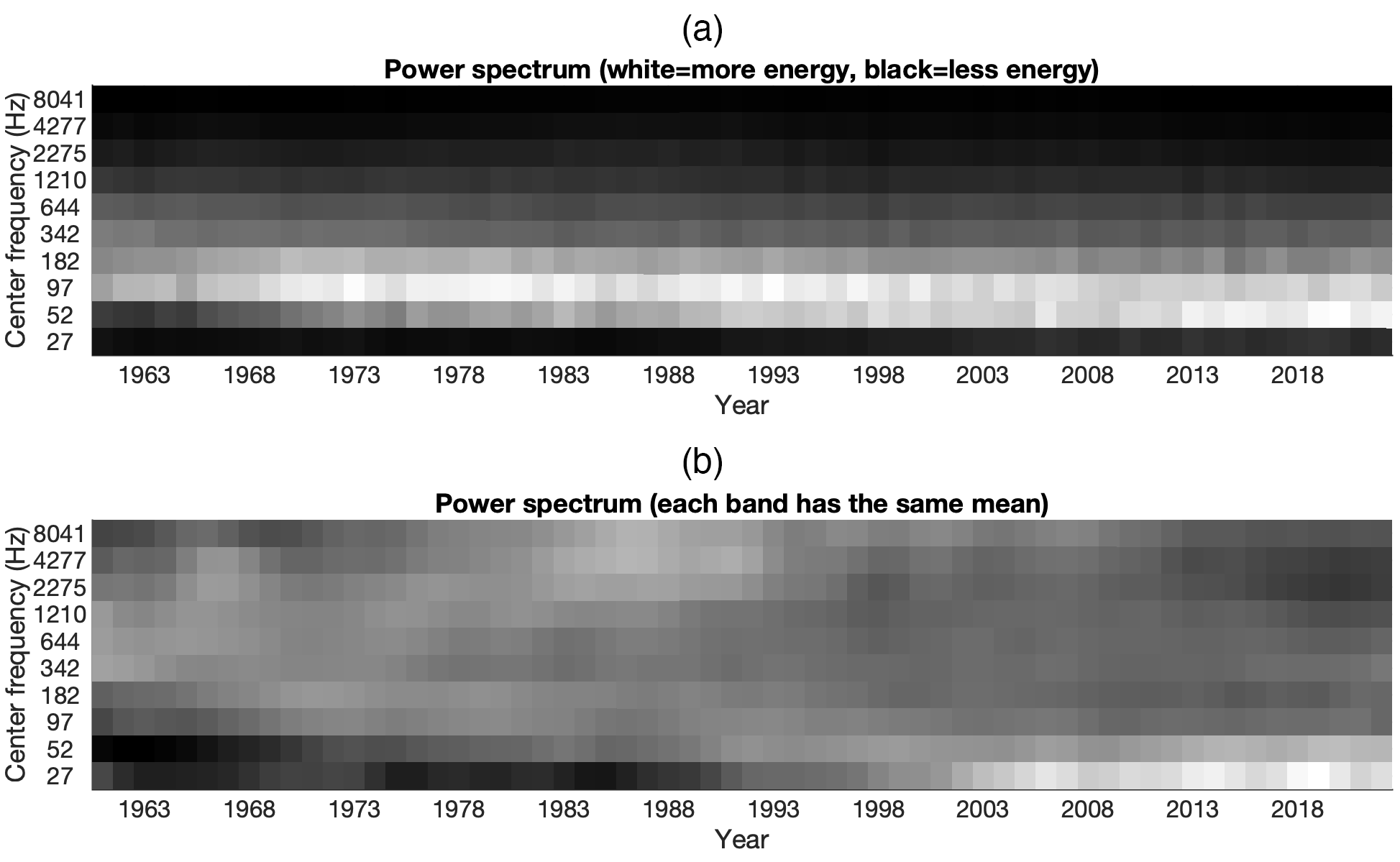
Figure 15: Power spectrum, BEA. (a) Spectrum for raw values. (b) Spectrum transformed so that values for each band have the same mean. The lower graph is blurred for better readability.

Figure 8 (section 4.5) shows the PC1 and PC2 values from weighted audio for the four datasets. One key difference between Figures 6 (original audio) and 8 (weighted audio) is that the four datasets are more clearly separated (obvious in the case of piano, orchestra, and popular music). The weighted data appears to be less long-tailed, with fewer outliers. We investigate to what extent this is the case. Figure 16 shows PC2 values according to the percentile to which the examples belong. The weighting process indeed reduces the proportion of outliers. Three examples of the phenomenon are shown in Figure 17:

• ‘Floor 555’, by XXXTentacion    This track results in exceptionally high PC1 and PC2 values. There exist other tracks from the dataset that do not sound so different from ‘Floor 555’ but that do not result in such extreme values. An example is ‘Surf Solar’ by band Fuck Buttons, which also features noisy elements around the high-medium frequencies and a solid rhythm track with a prominent kick drum. A close examination of ‘Floor 555’ shows that the extreme PC values result from low-frequency elements in the kick drum. Such elements cannot be heard at normal monitoring levels on most playback systems. Using weighted audio results in PC values that still correspond to inharmonic and noisy content but that are more commensurate to comparable-sounding tracks.

• ‘No gold teeth’ by Danger Mouse and ‘New tank’ by Playboi Carti    Both tracks have in common a loud, non-inharmonic bass, as well as higher frequency, more inharmonic elements. When weighted, the influence of the bass diminishes, and the relative inharmonicity (PC2) values are significantly increased.

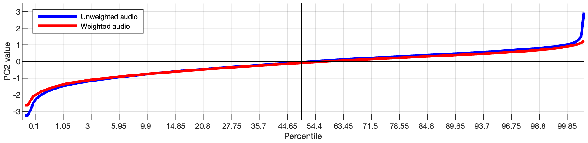
Figure 16: BEA dataset, PC2, unweighted and weighted audio, correspondence between percentiles and values.

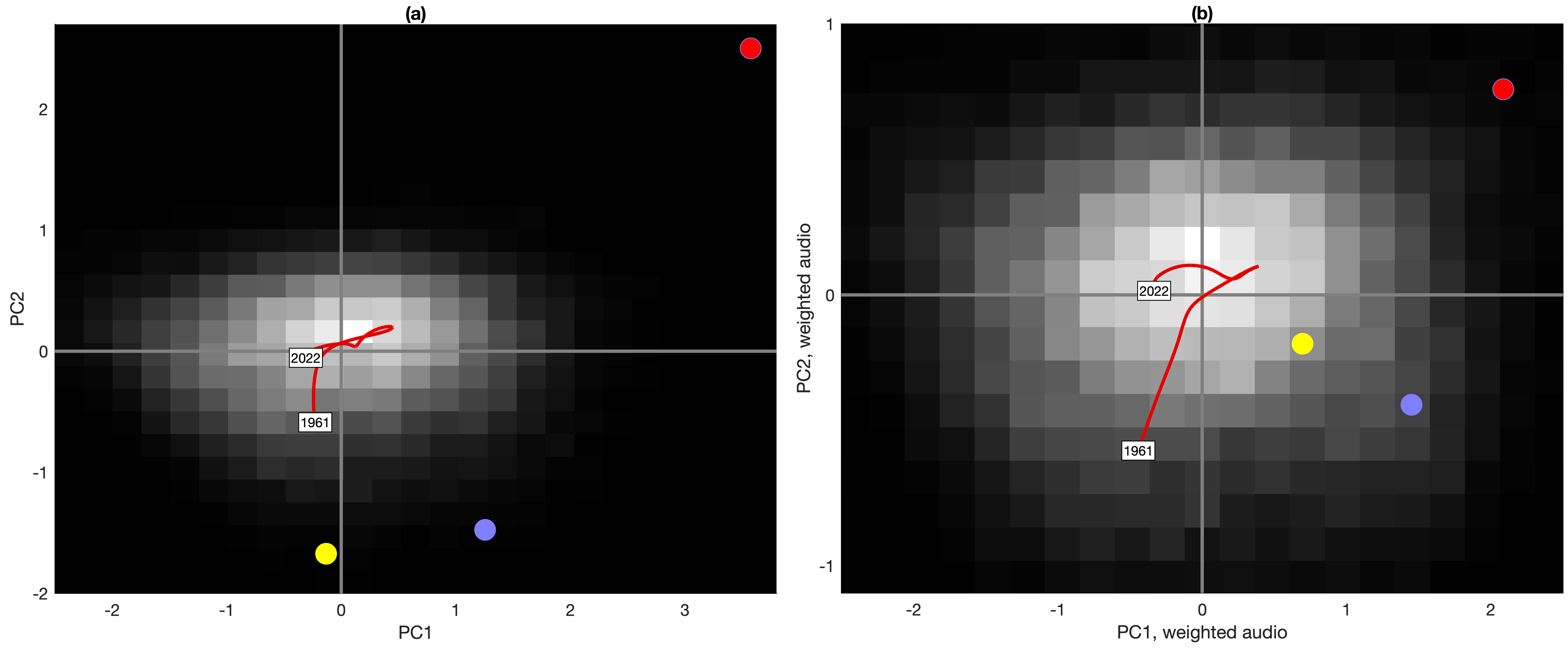
Figure 17: Positions of XXXTentacion’s ‘Floor 555’ (red), Danger Mouse’s ‘No gold teeth’ (blue), and Playboi Carti’s ‘New tank’ (yellow), in the representations from unweighted audio (a) and weighted audio (b).

Overall, we can observe a higher uniformity in terms of PC1 and PC2 when the corresponding content can be more easily perceived. In other words, music producers may be more conservative when they work with frequency bands for which the ear is more sensitive.

11 Analysis of specific tracks and artists

In this section, we focus on the music of particular artists using the analysis of weighted audio proposed in section 4.5. We suggest links between the analysis results and production methods.

11.1 Selected artists

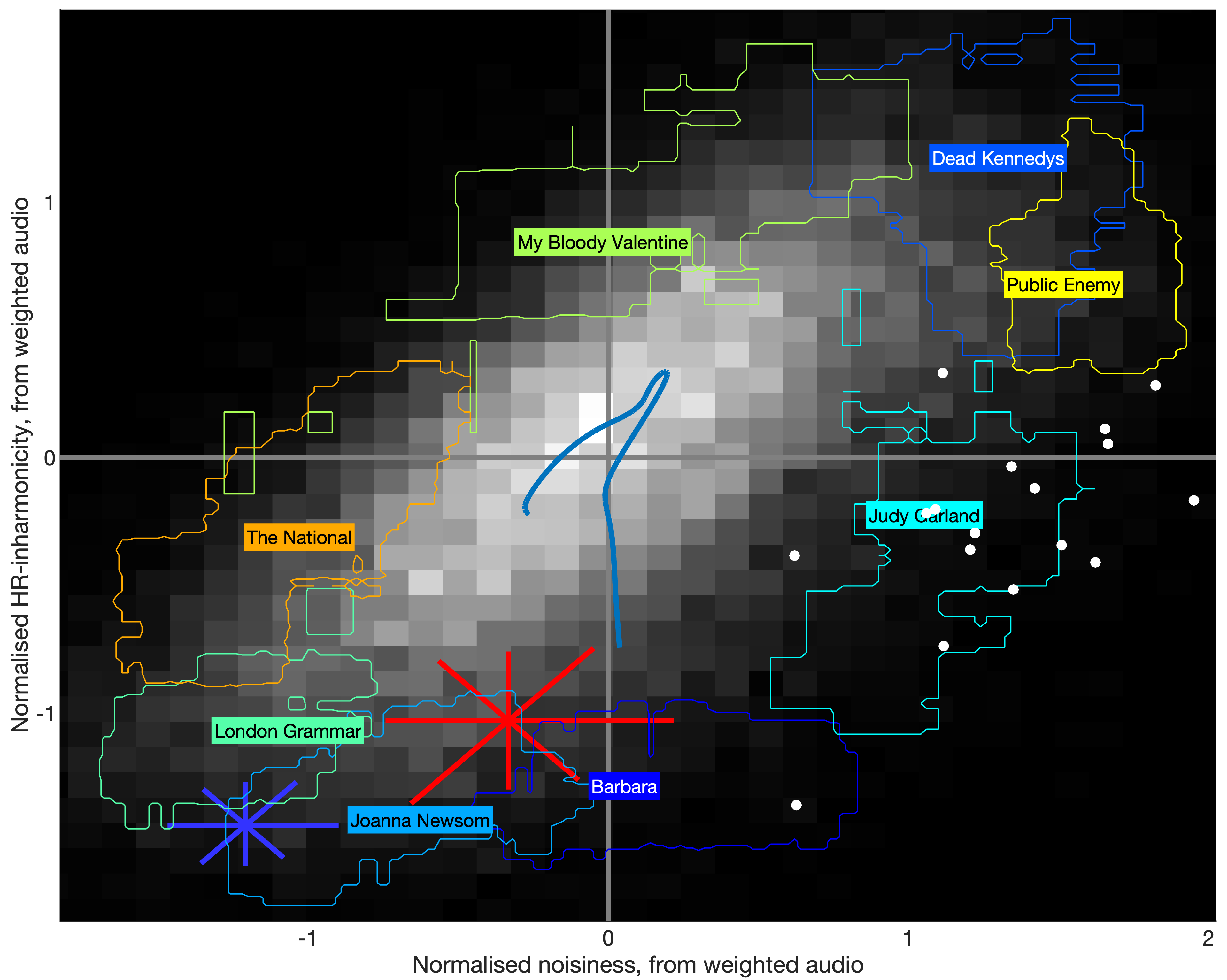
Figure 18: BEA dataset, normalised noisiness and HR-inharmonicity corresponding to particular artists as well as to monodic speech tracks. For each artist, the contours represent the isolines at half-height. Contours are evaluated on a mean filter of the distribution for better readability. The artist’s name is centered on the median. The white dots correspond to individual monodic and possibly processed speech tracks (the ‘skits’). The red and blue stars denote the feature distributions for the piano and orchestral music datasets, as in Figure 6.

Figure 18 illustrates noisiness and HR-inharmonicity values for several artists and speech tracks (weighted audio). Artists were chosen that lie on the edges of the distribution so that it is easier to understand the perceptual meaning of the two dimensions. Figure 19 shows the same data after PCA. We go through each element in Figures 18 and 19 so as to identify links between the feature values and aspects of the corresponding audio content.

1. Initial reference: speech tracks. The speech tracks in Figures 18 and 19 (white dots) are ‘interludes’ or ‘skits’ as found in hip-hop music. They generally have a low PC2 value. Low PC2 values for speech tracks illustrate how a sound can be non-inharmonic while not featuring stable pitch values. Higher PC2 values are observed in some of the examples of distorted voices. Higher PC1 values are observed in the examples that feature a high background noise.

2. PC2 values that are comparable to speech. The two artists whose music corresponds to PC2 values similar to those for speech are Barbara and Judy Garland. Their music features a monodic lead singer with piano and/or orchestral accompaniment. Drums may be present in Garland’s music but not in Barbara’s, which may account for the lower noisiness and PC1 values of the latter.

3. Exemplification of the 1961–1986 evolution. The combined evolution of PC1 and PC2 from 1961 to 1986 is exemplified by the production of the artist Barbara on the one hand, and the production of the band My Bloody Valentine on the other. The music of My Bloody Valentine is characterised by complex guitar textures involving open tuning (Leonard,, 2021), pitch bending and tremolo (Di Perna,, 1992), as well as an extensive effect rig (Double,, 1992). Listening to this music suggests that although chords seem to be identifiable, the perception of individual notes is difficult. This observation is consistent with (a) the fact that the tracks from the band feature a high amount of inharmonic relations between partials (top right of the PC1–PC2 representation) and (b) the conception according to which perception of pitch in inharmonic sounds is more ambiguous than in harmonic sounds (Schneider,, 2000; Schneider and Frieler,, 2009). According to the music critic Anthony Fantano, the ever-prominent guitar in ‘Loveless’, one of the band’s albums in the dataset, is ‘slathered with all of these seducing waves of pink smog, and these waves are so plentiful to the point where it obscures the guitar but also kind of make you see the guitar in a different light’. The examples of Barbara and My Bloody Valentine suggest that between 1961 and 1986, recorded music evolved in a general direction that goes from acoustic, tonal instruments playing content from a musical score (or, at least, that can be transcribed to a score), to heavily processed, noisy, and inharmonic content made in the recording studio and including drums.

   

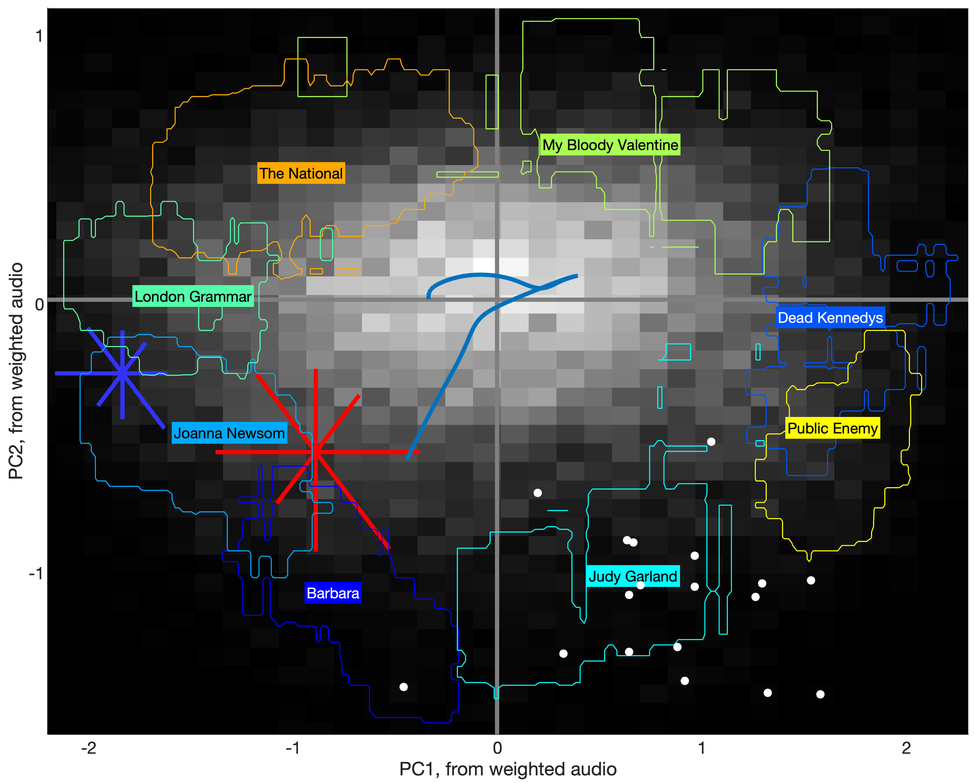
   Figure 19: Same data as in Figure 18, PCA.

4. Noise from distortion. The position of Dead Kennedys in Figures 18 and 19 indicates that they have very high total noise and inharmonicity and that the proportion of inharmonicity relative to noise is close to the median value for that level of noise. Dead Kennedys is a punk rock band from the 1980s whose music features noisy vocals, drums, bass, and distorted guitar. The noise is likely to originate from the vocals, drums, and guitar. Drums have a wide frequency range. In heavy-metal type distortion, the noise is not layered with the harmonics; it surrounds each harmonic (Berger and Fales,, 2005, p. 184). Figure 20 shows that noise in Dead Kennedys is indeed distributed on different frequencies. PC2 values are lower than in the case of My Bloody Valentine, possibly deriving from Dead Kennedys’ guitar parts mixed less loudly and containing fewer layers.

5. Exemplification of the 1986–2020 evolution. The combined evolution of PC1 and PC2 from 1986 to 2020 is exemplified by the production of the band Dead Kennedys on the one hand, and the production of the band London Grammar on the other. The inharmonicity to noise ratio is close to the median for the entire BEA dataset for both Dead Kennedys and London Grammar, but the total amount of noise and inharmonicity is very low for London Grammar and very high for Dead Kennedys. London Grammar is an indie pop band from the 2010s. The band’s music is studio and synth oriented (MusicTech,, 2023), carefully produced (Senior,, 2014) and inspired by atmospheric pieces (7Digital United States,, 2013). Listening to the music reveals lead vocals with smoothed plosives, noiseless but rich and multi-layered arrangements, and much reverb. The numerous layers and reverb may account for higher PC2 values than in the case of Joanna Newsom’s music. The examples of Dead Kennedys and London Grammar suggest that between 1986 and 2020, recorded music evolves in a general direction that goes from simpler and noisier tones to more polished, complex, and multi-layered studio works. The evolution in this direction is of lesser magnitude than the aforementioned evolution between 1961 and 1986.

6. Slightly inharmonic music based on acoustic instruments. The music of Joanna Newsom has a higher PC2 value than the music of Barbara, but lower total noise and inharmonicity. This means that the ratio of inharmonicity to noise is higher in Newsom’s music than in Barbara’s and that this higher ratio comes from inharmonic tones. Listening to Newsom’s music suggests that it features fewer layers than in the music of London Grammar. According to the interpretation of HarmonicRatio provided in section 6.3, fewer elements may result in less inharmonicity. Newsom’s music consists of vocals with mostly harp accompaniment, and sometimes piano and orchestra accompaniment. Higher PC2 values than Barbara’s music may result from the use of the harp. The harp is difficult to tune (Cathcart,, 2018) and features an initial ‘twang’ resulting in higher frequencies that converge to the target pitch (Fletcher,, 2000). Given the inharmonicity of piano strings (Rasch and Heetvelt,, 1985), such extensive use of the harp is consistent with Newsom’s proximity to the piano dataset values. The PC2 value for Newsom’s music is still below the median, meaning that the amount of inharmonicity relative to the level of noise is still lower than average. Low noisiness values may originate from the clean instrumentation, the relative absence of drums, as well as the lack of salient plosives in the vocal part.

7. Noise from sampling. The music of Public Enemy is as noisy as, but less inharmonic than, Dead Kennedys’ music. The two Public Enemy albums in the dataset were released in 1988 and 1990. The music results from the recombination of numerous samples over several layers (McLeod and DiCola,, 2011, pp. 22-26). It is ‘part musique concrete, […] a noisy collage of sputtering Uzis [a type of machine gun], wailing sirens, fragments of radio and TV commentary […], all riding on rhythms articulated by constantly changing drum voices […] Off-kilter loops, aliased or scratchy samples, and high-pitched spiraling sounds’ (Forman and Neal,, 2004, p. 408), accounting for the high noisiness. The lower inharmonicity-to-noise ratio than Dead Kennedys may derive from Public Enemy employing relatively fewer pitched elements. Like the music of Joanna Newsom, that of Public Enemy has a lower-than-average inharmonicity-to-noise ratio (PC2). However, in contrast to Newsom’s music, the total amount of inharmonicity and noise in Public Enemy’s music is very high (PC1).

8. Does studio work lead to more inharmonic partials? The music of The National is less noisy than that of My Bloody Valentine, with an almost equal proportion of inharmonicity deriving from partials. As in the case of My Bloody Valentine, the production work involves much studio experimentation (Doyle,, 2017). The band features two guitarists, who make use of extensive pedal-boards and place ‘more importance on textural soundscaping than [virtuosity]’. One goal of the band is to create a ‘lattice work of notes’ (Guitar.com,, 2017). An example of a method leading to such a result resides in the album ‘Sleep Well Beast’, where ‘the pianos are playing off each other by an eighth note’ (Guitar.com,, 2017). Such a process will increase the number of simultaneous pitch values. Considering, as seen previously, that more numerous different tones result in more inharmonicity, such methods may contribute to increasing inharmonicity values. Much sustain and reverb will also lead to increased inharmonicity because of tones that are close together in pitch in the same part or voice overlapping in time.

Figure 20: Band-by-band normalised noisiness for the Dead Kennedys’ music. The gray rectangles represent the noisiness values for the entire dataset (25^th, 50^th and 75^th percentiles), adjusted so that the median is zero. The red rectangles represent the adjusted noisiness values for Dead Kennedys.

A key observation from the above is that low PC2 values appear to correspond to tonal music with clearly distinguishable elements (Barbara, Judy Garland). If we consider the gradation from low to high PC2 values on the low PC1 side (Barbara, Joanna Newson, London Grammar, The National), then the music appears to gradually involve more and more studio work. This would result in keeping the total amount of inharmonicity and noise roughly constant (and low) and increasing the ratio of inharmonicity to noise, which means increasing the extent to which inharmonicity results from partials rather than noise. High PC2 values seem to correspond to music in which heavy studio production work is performed on ‘pitched’ instruments, especially on guitars (The National, My Bloody Valentine).

11.2 Possible causes for high PC1 and PC2 values

PC1 values are generally higher in the case of popular music than in the case of orchestral music (see section 4, Figures 6 and 8, as well as Figure 21 below). Possible factors for higher PC1 values may involve loud drums (Dead Kennedys, Public Enemy), distortion (Dead Kennedys, My Bloody Valentine), noisy samples (Public Enemy), and vocals with loud plosives (Dead Kennedys, Public Enemy).

PC2 values are also generally higher in the case of CPM than in the case of orchestral music. As PC2 is the ratio of inharmonicity to noise, a higher PC2 value indicates that noise makes a relatively smaller contribution to the total sum of inharmonicity and noisiness (i.e., to PC1). As previously stated, lower HarmonicRatio values may be obtained either from properties deriving from each complex tone (e.g., inharmonicity) or from properties deriving from the combination of complex tones (e.g., number of sources and scales). Judging from the facts that (1) orchestras have a high number of sources, and (2) harmony in CPM does not appear to be more chromatic than that of Western classical music, we might conclude that the higher PC2 values in CPM originate from tone inharmonicity.

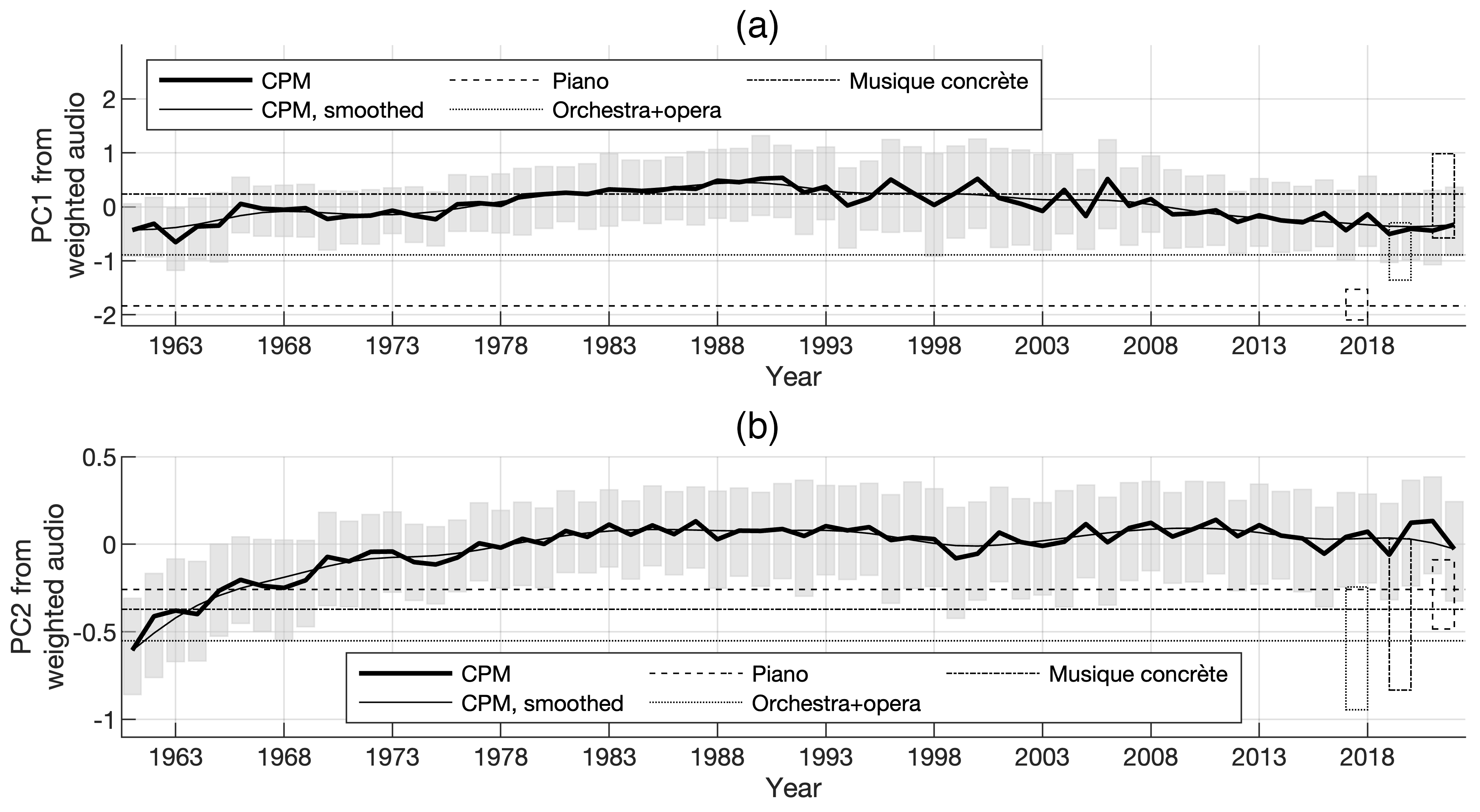
Figure 21: Measures of (a) PC1 and (b) PC2 from weighted audio for the four datasets.

11.3 High inharmonicity—to what extent?

Given that we perform the analysis on final stereo tracks, it is difficult to verify this conclusion in the general case. However, it is possible to analyse a particular example to understand one way to reach high PC2 values. The song ‘Sometimes’ by My Bloody Valentine features particularly high PC2 values. At the end of the song, a solo guitar chord corresponds to even higher PC2 values. We isolate this part and evaluate its power spectrum. Figure 22, top, shows that the part is a quasi-harmonic 37.5Hz complex tone with its fundamental missing. Figure 22, middle, shows that the relative loudness of the overtones is high, which explains why this single complex tone was initially perceived as a chord: we hear some of the overtones as independent notes. Figure 22, bottom, shows the frequency difference between consecutive partials. The difference is not constant, which makes the complex tone strongly inharmonic.

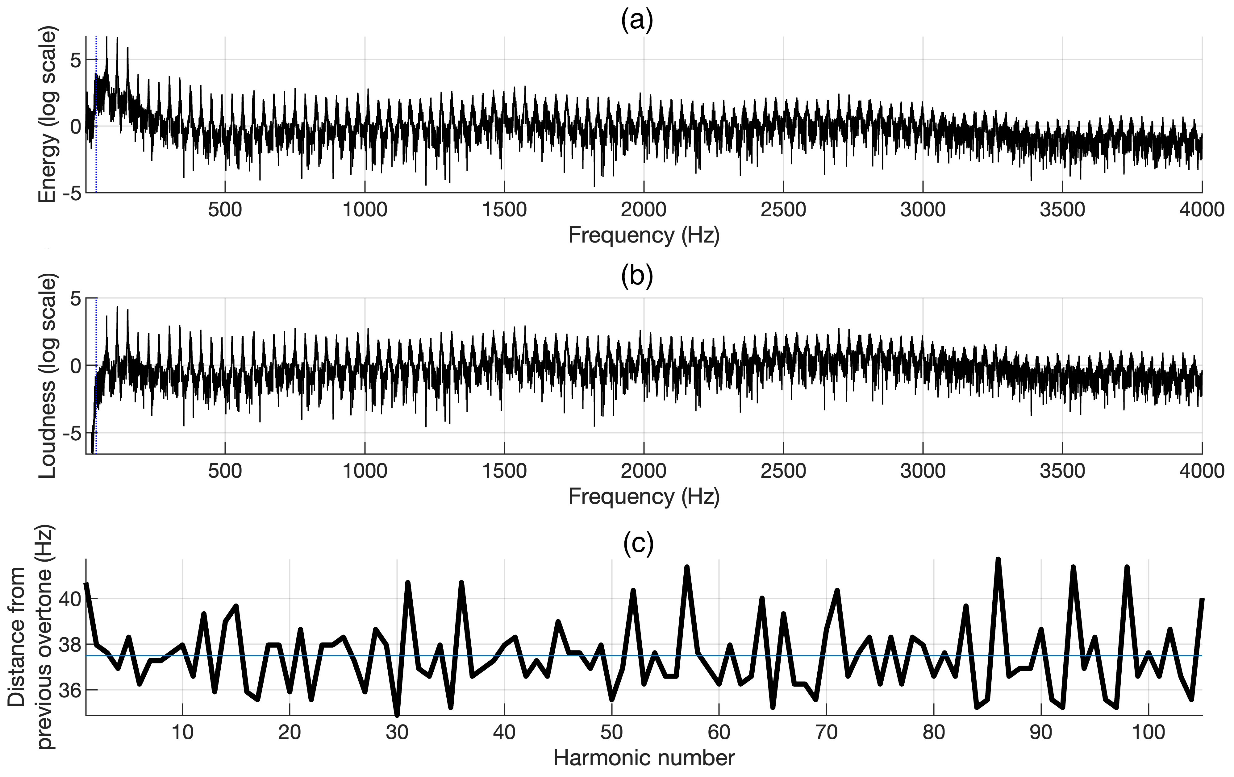
Figure 22: Excerpt from My Bloody Valentine, ‘Sometimes’, from the album ‘Loveless’. The excerpt’s timing is 5’06 to 5’19. (a) Power spectrum. (b) Power spectrum weighted with ISO226:2003, 50 phon. (c) Distance between the harmonics. The mean frequency difference between consecutive partials (37.5Hz) is drawn in the top and middle diagram as the blue dotted line.

Such properties of the signal are not specific to this particular song. For instance, we can witness a similar tone architecture in the keyboard part at the end of Alt-J’s ‘Hunger Of The Pine’—albeit with fewer inharmonic overtones. It is also worth noting that ‘Loveless’ has been highly influential, being an inspiration to artists such as The Verve, Oasis, Deerhunter, M83, DIIV, Deafheaven and Coldplay (Hudson,, 2021). It is rated by BestEverAlbums.com as the second best album of 1991, second only to the extremely successful ‘Nevermind’ by Nirvana.

Schneider and Frieler, (2009) studied inharmonicity in bells from the belfry of Brugge. They remark that the SPINET pitch detection algorithm (Cohen et al.,, 1995) fails to provide interpretable results in single bell samples. They also note that using bells as instruments ‘hampers [human] detection of the pitches’, which in turn prevents the following of voices as well as the understanding of tonal functions. One question that therefore arises is to what extent inharmonicity in CPM hampers or even prevents the algorithmic detection of pitch, the following of voices, and the understanding of tonal functions. We compare PC1 and PC2 values corresponding to bells from Dutch belfries with the values corresponding to the BEA dataset. The results are shown in Figure 23. Bells generally have higher PC1 and PC2 values than popular music. However, the values corresponding to the complex tone showcased in Figure 22 are above the median values corresponding to bell samples in both cases. This complex tone involves a higher total amount of noise and inharmonicity (PC1) and a higher proportion of noise and inharmonicity that is due to inharmonic intervals between partials (PC2) than most bell sounds, which results in more inharmonic relations between partials. It suggests that in CPM, at least some instruments (in this case, the electric guitar, which is not a marginal instrument) may result in enough inharmonic relations between partials to prevent human and algorithmic identification of pitch. The conclusion is relevant to one initial interrogation mentioned in section 2: in CPM, to what extent are pitched elements harmonic?

Figure 23: Comparison of normalised (a) PC1 and (b) PC2 values from weighted audio: bells, BEA dataset, and end part of My Bloody Valentine’s ‘Sometimes’.

12 Conclusions

The initial question, as introduced in section 1 and elaborated upon in section 5.3, can be phrased as follows: given that recent popular music, unlike Western classical music, is not subject to the constraint of (almost exclusively) using acoustic resonators (as employed in acoustic instruments), to what extent do the two music categories differ in terms of properties that can be related to the use of acoustic resonators? The short answer to this question is that recent popular music is both noisier and more inharmonic than Western classical music (section 4, Figures 6 and 8). It is also more inharmonic than musique concrète and slightly less noisy.

We now summarise the methods on which the study is based.

1. We directly derived the HR-inharmonicity feature (section 3.2.1, detailed in section 6) from the MPEG-7’s HarmonicRatio feature, which in turn has been used to measure pitch strength.

2. We used the noisiness feature (section 3.2.2, detailed in section 7), derived from the MPEG-7’s AudioFlatnessType feature, primarily characterised as being the opposite of peak prominence. Noisiness denotes a locally ‘flat’ spectrum.

3. We argued that as the human ear is not equally sensitive to all frequencies, weighting the audio using equal loudness contours prior to feature evaluation can provide results that better reflect what a human listener actually hears (section 3.2.4, detailed in section 10). Measures showed that the weighting increases the proximity of perceptually similar tracks and reduces the number of outliers.

4. As HR-inharmonicity and noisiness are not independent of each other (section 3.2.3, detailed in section 6.6), we used PCA to define two new features, PC1 and PC2. PC2 is particularly significant, as it measures the proportion of inharmonicity that is due to inharmonic relations between partials and not to noise. It follows that it also measures the respective contribution of inharmonic relations between partials and noise in pitch strength.

We now summarise the main findings of the study.

1. We showed that HR-inharmonicity of popular music is comparable to that of musique concrète (section 4.1). At the beginning of the 1960s, it was similar to that of Western orchestral music, and it then increased to reach a peak in the mid-1980s. In section 6, we showed that high HR-inharmonicity values, and, therefore, low pitch strength, may derive from noise and/or interaction between inharmonically related partials within and between complex tones. In the latter case, the degree of inharmonicity depends on both the proximity and energy of interacting partials. We also showed that higher HR-inharmonicity values prompt faster acoustic beating.

2. We showed that noisiness of popular music is comparable to that of Western orchestral music and lower than that of musique concrète (section 4.2). It reaches a maximum during the mid-1980s.

3. In regards to the frequencies to which humans are the most sensitive, popular music is generally slightly noisier and considerably more HR-inharmonic (lesser pitch strength) than orchestral music (section 4.4). The total amount of HR-inharmonicity and noisiness combined (PC1) is greater on average in popular music than in Western classical music.

4. The proportion of HR-inharmonicity that is due to inharmonic relations between partials for popular music at the beginning of the 1960s was comparable to that of orchestral music (section 4.4). It then increased rapidly until ca. 1972. Later evolutions are slower. It was therefore suggested that popular music released after the evolution forms a category of its own, which we proposed to refer to as ‘Contemporary Popular Music’ (CPM). CPM may be characterised by a density of inharmonic relations between partials that is, on average, significantly higher than that of music from other categories.

We linked feature values with examples drawn from the popular music dataset (sections 11.1 and 11.2) and observed the following:

1. High noisiness values appear to be easy to link with the audio content. Noise may be heard in drums, vocal plosives, distortions, and ‘real-life’ noisy ambiances.

2. HR-inharmonicity and PC2 are more difficult to pinpoint. We formulated the hypothesis according to which high HR-inharmonicity and PC2 values may derive from the use of ‘tonal’ sounds coupled with intensive use of the studio. Such use of the studio may be specific to CPM, as musique concrète, another category of studio-based music, is both noisier and less HR-inharmonic.

We were able to draw other conclusions that are not direct answers to the initial question but may remain useful in the context of the domain of music information retrieval:

1. While high inharmonicity values may originate from both the intervals between complex tones and the inharmonicity of individual complex tones, increasing the inharmonicity of individual complex tones reduces the relative influence on inharmonicity of the intervals between complex tones (section 6.4).

2. According to Peeters, (2004, p. 20), ‘Spectral Flatness is a measure of the noisiness (flat, decorrelation)/sinusoidality of a spectrum’. According to (ISO,, 2001, p. 26), ‘[t]his descriptor expresses the deviation of the signal’s power spectrum over frequency from a flat shape (corresponding to a noise-like or an impulse-like signal). A high deviation from a flat shape may indicate the presence of tonal components’. According to the Essentia documentation, spectral flatness is ‘a measure of how noise-like a sound is, as opposed to being tone-like’. However, we showed that if one considers that pink noise and white noise should both result in high noisiness values, which may better correspond to the intuitive notion of ‘noisiness’, the overall spectral envelope should be filtered out prior to spectral flatness evaluation (section 7).

3. In terms of noisiness and inharmonicity, we could not find the effects of the ‘homogenization of the timbral palette’ reported by Serrà et al., (2012). On the contrary, the transition towards CPM shows a significant increase in the diversity of noisiness and inharmonicity values, which evolves to be greater than that of orchestral music (section 9).

4. The output of feature-based studies may be made more reliable by attenuating the influence of audio frequencies human listeners are less sensitive to (section 10). In particular, the weighting function gives relatively much less weight to the lower frequencies. This suggests that it may be useful to weigh the initial signal using models such as ISO226:2003 (ISO,, 2003).

Finally, in section 11.3, we compared HR-inharmonicity and PC2 in popular music and church bells. Although church bells generally involve more inharmonic relations between partials than popular music, it may be that some instruments in popular music tracks result in more inharmonic relations between partials than most church bells. Given that inharmonicity in bells hampers automatic pitch detection and human perception of pitch, it is possible that as a consequence of the use of specific resources of the performances, some instruments in popular music, such as the electric guitar, may result in content that is inharmonic enough to make it unsuitable for analysis and description as musical notes. Using the terms introduced in sections 5.1 and 5.3, idioms of popular music may not always involve musical notes, even when the elements on which the idioms are based involve waveforms that feature a strongly periodic behaviour and convey an impression of pitch. This is a topic we intend to explore further in future studies.

Disclosure statement

The authors report there are no competing interests to declare.

References

- 7Digital United States, (2013) 7Digital United States (2013). London Grammar Interview.
- Barbieri, (2002) Barbieri, P. (2002). La nascita delle teorie ’continue’ della consonanza. La ignorata curva di Draghetti e Foderà, poi di Helmholtz (1771–1837). Acta Musicologica, 74(Fasc. 1):55–75.
- Barbour, (2004) Barbour, J. M. (2004). Tuning and temperament: A historical survey. Courier Corporation.
- Bell, (2014) Bell, A. P. (2014). Trial-by-fire: A case study of the musician–engineer hybrid role in the home studio. Journal of Music, Technology & Education, 7(3):295–312.
- Benetos et al., (2018) Benetos, E., Dixon, S., Duan, Z., and Ewert, S. (2018). Automatic music transcription: An overview. IEEE Signal Processing Magazine, 36(1):20–30.
- Bent, (2001) Bent, I. D. (2001). Notation. Grove Music Online.
- Berger and Fales, (2005) Berger, H. M. and Fales, C. (2005). ’heaviness’ in the perception of heavy metal guitar timbres: The match of perceptual and acoustic features over time. Wired for Sound: Engineering and Technologies in Sonic Cultures, pages 181–197.
- Bertin-Mahieux et al., (2011) Bertin-Mahieux, T., Ellis, D. P., Whitman, B., and Lamere, P. (2011). The million song dataset. In 12th International Society for Music Information Retrieval Conference (ISMIR 2011).
- Bogdanov et al., (2013) Bogdanov, D., Wack, N., Gómez Gutiérrez, E., Gulati, S., Boyer, H., Mayor, O., Roma Trepat, G., Salamon, J., Zapata González, J. R., Serra, X., et al. (2013). Essentia: An audio analysis library for music information retrieval. In Britto A, Gouyon F, Dixon S, editors. 14th Conference of the International Society for Music Information Retrieval (ISMIR); 2013 Nov 4-8; p. 493-8. International Society for Music Information Retrieval (ISMIR).
- Brandt et al., (2019) Brandt, M., Doclo, S., and Bitzer, J. (2019). Automatic noise psd estimation for restoration of archived audio. Journal of the Audio Engineering Society, 67(1/2):38–53.
- Campbell, (2001) Campbell, M. (2001). Inharmonicity. Grove Music Online.
- Cathcart, (2018) Cathcart, C. (2018). Ringing strings - you can’t tune a harp. Folk Harp Journal, 180.
- Charlton and Whitney, (2001) Charlton, D. and Whitney, K. (2001). Score (i). Grove Music Online.
- Cohen et al., (1995) Cohen, M. A., Grossberg, S., and Wyse, L. L. (1995). A spectral network model of pitch perception. The Journal of the Acoustical Society of America, 98(2):862–879.
- de Boer, (1956) de Boer, E. (1956). Pitch of inharmonic signals. Nature, 178(4532):535–536.
- Deruty, (2011) Deruty, E. (2011). Dynamic range and the loudness war. Sound on Sound–September 2011, pages 22–24.
- Deruty et al., (2022) Deruty, E., Grachten, M., Lattner, S., Nistal, J., and Aouameur, C. (2022). On the development and practice of AI technology for contemporary popular music production. Transactions of the International Society for Music Information Retrieval, 5(1).
- Deruty and Pachet, (2015) Deruty, E. and Pachet, F. (2015). The MIR perspective on the evolution of dynamics in mainstream music. In Proceedings of the 16th ISMIR Conference, volume 723.
- Di Perna, (1992) Di Perna, A. (1992). Bloody guy. Guitar World.
- Double, (1992) Double, S. (1992). Kevin Shields, My Bloody Valentine Interview. New Musical Express.
- Doyle, (2017) Doyle, T. (2017). The national. aaron dessner and jonathan low: Recording sleep well beast. Sound on Sound.
- Ewert et al., (2012) Ewert, S., Muller, M., Konz, V., Mullensiefen, D., and Wiggins, G. A. (2012). Towards cross-version harmonic analysis of music. IEEE Transactions on Multimedia, 14(3):770–782.
- Ewert et al., (2014) Ewert, S., Pardo, B., Muller, M., and Plumbley, M. D. (2014). Score-informed source separation for musical audio recordings: An overview. IEEE Signal Processing Magazine, 31(3):116–124.
- Favreau et al., (2010) Favreau, E., Geslin, Y., and Lefèvre, A. (2010). L’acousmographe 3. In Journées d’Informatique Musicale - 2010, Rennes, France.
- Fine, (2008) Fine, T. (2008). The dawn of commercial digital recording. ARSC Journal, 39(1):1–17.
- Fitzgerald, (2010) Fitzgerald, D. (2010). Harmonic/percussive separation using median filtering. In Proc. of the 13th Int. Conference on Digital Audio Effects (DAFx-10), Graz, Austria, September 6-10, 2010.
- Fletcher et al., (1962) Fletcher, H., Blackham, E. D., and Stratton, R. (1962). Quality of piano tones. The Journal of the Acoustical Society of America, 34(6):749–761.
- Fletcher and Munson, (1933) Fletcher, H. and Munson, W. A. (1933). Loudness, its definition, measurement and calculation. Bell System Technical Journal, 12(4):377–430.
- Fletcher, (2000) Fletcher, N. (2000). Inharmonicity, nonlinearity and music. The Physicist, 37(5):171–175.
- Fletcher and Rossing, (2012) Fletcher, N. H. and Rossing, T. D. (2012). The physics of musical instruments. Springer Science & Business Media.
- Forman and Neal, (2004) Forman, M. and Neal, M. A. (2004). That’s the joint!: the hip-hop studies reader. Psychology Press.
- Frith, (2004) Frith, S. (2004). Popular music: Critical concepts in media and cultural studies, volume 1. Psychology Press.
- Gómez, (2006) Gómez, E. (2006). Tonal description of music audio signals. Department of Information and Communication Technologies.
- Guitar.com, (2017) Guitar.com (2017). Interview: The national – national anthems. Guitar.com.
- Helmholtz and Ellis, (1885) Helmholtz, H. L. F. v. and Ellis, A. J. (1885). On the sensations of tone as a physiological basis for the theory of music. Longmans, Green, and Co.
- Hove et al., (2019) Hove, M. J., Vuust, P., and Stupacher, J. (2019). Increased levels of bass in popular music recordings 1955–2016 and their relation to loudness. The Journal of the Acoustical Society of America, 145(4):2247–2253.
- Hsu and Jang, (2009) Hsu, C.-L. and Jang, J.-S. R. (2009). On the improvement of singing voice separation for monaural recordings using the mir-1k dataset. IEEE transactions on audio, speech, and language processing, 18(2):310–319.
- Huang et al., (2020) Huang, C.-Z. A., Koops, H. V., Newton-Rex, E., Dinculescu, M., and Cai, C. J. (2020). AI song contest: Human-AI co-creation in songwriting. In 21st International Society for Music Information Retrieval Conference (ISMIR 2020).
- Hudson, (2021) Hudson, A. (2021). ’Loveless’ at 30: Zoon Reflects on the Influence of My Bloody Valentine’s Shoegaze Blueprint. Exlaim.ca.
- Huron, (2001) Huron, D. (2001). Tone and voice: A derivation of the rules of voice-leading from perceptual principles. Music Perception, 19(1):1–64.
- Huron and Berec, (2009) Huron, D. and Berec, J. (2009). Characterizing idiomatic organization in music: A theory and case study of musical affordances. Empirical Musicology Review, 4(1):103–122.
- Hutchinson and Knopoff, (1978) Hutchinson, W. and Knopoff, L. (1978). The acoustic component of western consonance. Journal of New Music Research, 7(1):1–29.
- ISO, (2001) ISO (2001). ISO/MPEG N4224. International Standard 15938-4 Information Technology - Multimedia Content Description Interface - Part 4 Audio.
- ISO, (2003) ISO (2003). Normal equal-loudness level contours-ISO 226: 2003.
- Kim et al., (2018) Kim, J. W., Salamon, J., Li, P., and Bello, J. P. (2018). Crepe: A convolutional representation for pitch estimation. In 2018 IEEE International Conference on Acoustics, Speech and Signal Processing (ICASSP), pages 161–165. IEEE.
- Klapuri, (2003) Klapuri, A. P. (2003). Multiple fundamental frequency estimation based on harmonicity and spectral smoothness. IEEE Transactions on speech and audio processing, 11(6):804–816.
- Lavengood, (2017) Lavengood, M. (2017). A new approach to the analysis of timbre. City University of New York.
- Leonard, (2021) Leonard, M. (2021). How Kevin Shields and My Bloody Valentine changed the course of guitar playing forever. Guitar.com.
- Masina et al., (2022) Masina, I., Presti, G. L., and Stanzial, D. (2022). Dyad’s consonance and dissonance: combining the compactness and roughness approaches. The European Physical Journal Plus, 137(11):1254.
- Mattis, (2001) Mattis, O. (2001). Chowning, John M(acLeod). Grove Music Online.
- Mauch and Dixon, (2010) Mauch, M. and Dixon, S. (2010). Approximate note transcription for the improved identification of difficult chords. In ISMIR, pages 135–140.
- Mauch et al., (2015) Mauch, M., MacCallum, R. M., Levy, M., and Leroi, A. M. (2015). The evolution of popular music: Usa 1960–2010. Royal Society open science, 2(5):150081.
- Mazzanti, (2019) Mazzanti, S. (2019). Defining popular music: Towards a “historical melodics”. Contemporary Popular Music Studies: Proceedings of the International Association for the Study of Popular Music 2017, pages 17–26.
- McCartney and Miles, (1997) McCartney, P. and Miles, B. (1997). Paul McCartney: many years from now. Secker & Warburg, London, UK.
- McLeod and DiCola, (2011) McLeod, K. and DiCola, P. (2011). Creative license: The law and culture of digital sampling. Duke University Press, Durham, USA.
- McPherson and Tahıroğlu, (2020) McPherson, A. and Tahıroğlu, K. (2020). Idiomatic patterns and aesthetic influence in computer music languages. Organised sound, 25(1):53–63.
- Micheyl and Oxenham, (2010) Micheyl, C. and Oxenham, A. J. (2010). Pitch, harmonicity and concurrent sound segregation: Psychoacoustical and neurophysiological findings. Hearing research, 266(1-2):36–51.
- Middleton, (1990) Middleton, R. (1990). Studying popular music. McGraw-Hill Education (UK).
- Milner, (2011) Milner, G. (2011). Perfecting sound forever: The story of recorded music. Granta Books.
- Moreau et al., (2006) Moreau, N., Sikora, T., and Kim, H.-G. (2006). MPEG-7 audio and beyond: Audio content indexing and retrieval. John Wiley & Sons.
- Mowitt, (2002) Mowitt, J. (2002). Percussion: drumming, beating, striking. Duke University Press.
- Moylan, (2014) Moylan, W. (2014). Understanding and crafting the mix: The art of recording. CRC Press.
- Mumma et al., (2001) Mumma, Gordon, H. R., Kernfeld, B., and Sheridan, C. (2001). Recording. Grove Music Online.
- MusicTech, (2023) MusicTech (2023). My Forever Studio S5 E1: Dot Major doesn’t drag and drop beats.
- Ono et al., (2008) Ono, N., Miyamoto, K., Kameoka, H., and Sagayama, S. (2008). A real-time equalizer of harmonic and percussive components in music signals. In ISMIR, pages 139–144.
- Orton, (2001) Orton, R. (2001). Ondes martenot. Grove Music Online.
- Parry, (1911) Parry, C. H. H. (1911). Style in musical art. Macmillan, London, UK.
- Pascall, (2001) Pascall, R. (2001). Style. Grove Music Online.
- Patterson et al., (1996) Patterson, R. D., Handel, S., Yost, W. A., and Jaysurya Datta, A. (1996). The relative strength of the tone and noise components in iterated rippled noise. The Journal of the Acoustical Society of America, 100(5):3286–3294.
- Peeters, (2004) Peeters, G. (2004). A large set of audio features for sound description (similarity and classification) in the cuidado project. CUIDADO Ist Project Report, 54(0):1–25.
- Pestana et al., (2013) Pestana, P. D., Ma, Z., Reiss, J. D., Barbosa, A., and Black, D. A. (2013). Spectral characteristics of popular commercial recordings 1950-2010. In Audio Engineering Society Convention 135. Audio Engineering Society.
- Plomp and Levelt, (1965) Plomp, R. and Levelt, W. J. M. (1965). Tonal consonance and critical bandwidth. The journal of the Acoustical Society of America, 38(4):548–560.
- Porcaro, (2001) Porcaro, A. F. (2001). Moog, Robert A(rthur). Grove Music Online.
- Pras et al., (2013) Pras, A., Guastavino, C., and Lavoie, M. (2013). The impact of technological advances on recording studio practices. Journal of the American Society for Information Science and Technology, 64(3):612–626.
- Raffel, (2016) Raffel, C. (2016). Learning-based methods for comparing sequences, with applications to audio-to-midi alignment and matching. 2016.
- Raffel and Ellis, (2016) Raffel, C. and Ellis, D. P. (2016). Optimizing dtw-based audio-to-midi alignment and matching. In 2016 IEEE International Conference on Acoustics, Speech and Signal Processing (ICASSP), pages 81–85. IEEE.
- Rasch and Plomp, (1982) Rasch, R. and Plomp, R. (1982). The perception of musical tones. In Deutsch, D., editor, The Psychology of Music, pages 1–24. Academic Press, 1st edition.
- Rasch and Heetvelt, (1985) Rasch, R. A. and Heetvelt, V. (1985). String inharmonicity and piano tuning. Music Perception, 3(2):171–189.
- Riou et al., (2023) Riou, A., Lattner, S., Hadjeres, G., and Peeters, G. (2023). Pesto: Pitch estimation with self-supervised transposition-equivariant objective. arXiv preprint arXiv:2309.02265.
- Rose, (1996) Rose, F. (1996). Introduction to the pitch organization of french spectral music. Perspectives of New Music, pages 6–39.
- Salamon et al., (2017) Salamon, J., Bittner, R. M., Bonada, J., Bosch, J. J., Gómez Gutiérrez, E., and Bello, J. P. (2017). An analysis/synthesis framework for automatic f0 annotation of multitrack datasets. In Hu X, Cunningham SJ, Turnbull D, Duan Z. ISMIR 2017 Proceedings of the 18th International Society for Music Information Retrieval Conference; 2017 Oct 23-27; Suzhou, China.[Suzhou]: ISMIR; 2017. International Society for Music Information Retrieval (ISMIR).
- Schaeffer, (1966) Schaeffer, P. (1966). Traité des objets musicaux. Editions du Seuil. Paris, France.
- Schaeffer, (2020) Schaeffer, P. (2020). La musique concrète. PUF. Paris, France.
- Schneider, (2000) Schneider, A. (2000). Inharmonic sounds: Implications as to ’pitch’, ’timbre’ and ’consonance’. Journal of New Music Research, 29(4):275–301.