On the Spectral Efficiency of Movable and Rotary Access Points under Rician Fading

Abstract

Multi-User Multiple-Input Multiple-Output (MU-MIMO) is a pivotal technology in present-day wireless communication systems. In such systems, a base station or Access Point (AP) is equipped with multiple antenna elements and serves multiple active devices simultaneously. Nevertheless, most of the works evaluating the performance of MU-MIMO systems consider APs with static antenna arrays, that is, without any movement capability. Recently, the idea of APs and antenna arrays that are able to move have gained traction among the research community. Many works evaluate the communications performance of antenna systems able to move on the horizontal plane. However, such APs require a very bulky, complex and expensive movement system. In this work, we propose a simpler and cheaper alternative: the utilization of rotary APs, i.e. APs that can rotate. We also analyze the performance of a system in which the AP is able to both move and rotate. The movements and/or rotations of the APs are computed in order to maximize the mean per-user achievable spectral efficiency, based on estimates of the locations of the active devices and using particle swarm optimization. We adopt a spatially correlated Rician fading channel model, and evaluate the resulting optimized performance of the different setups in terms of mean per-user achievable spectral efficiencies. Our numerical results show that both the optimal rotations and movements of the APs can provide substantial performance gains when the line-of-sight components of the channel vectors are strong. Moreover, the simpler rotary APs can outperform the movable APs when their movement area is constrained.

I Introduction

Multi-User Multiple-Input Multiple-Output (MU-MIMO) technologies play a crucial role in contemporary wireless communication networks such as 4G LTE Advanced [1], 5G NR [2] and WiFi 6 [3]. In MU-MIMO networks, a base station or Access Point (AP) equipped with multiple antennas serve multiple active devices at the same time. By utilizing beamforming techniques, MU-MIMO provides numerous benefits, including diversity and array gains, spatial multiplexing capabilities, and interference suppression. These benefits collectively enhance the capacity, reliability, and coverage of wireless networks [4].

The vast majority of works investigating the performance of MU-MIMO networks consider APs equipped with fixed antenna arrays, i.e., antenna arrays with no movement capabilities. Nevertheless, the idea of antenna arrays that are able to move has gained attention among the research community, since some recent works have shown that antenna movements can substantially improve the quality of wireless links [5, 6, 7, 8, 9, 10, 11]. Some of their contributions will be discussed in the following subsection.

I-A Related Works

The utilization of antenna arrays with movement capabilities is not something new. For instance, authors in [12] proposed a Direction of Arrival (DOA) estimation method that utilizes a rotary Uniform Linear Array (ULA) of antennas. The rotary ULA presents satisfactory performance for under-determined DOA estimations, where the number of source signals can be larger than the number of receive antenna elements. The performance of point-to-point Line-of-Sight (LoS) links where both the transmitter and receiver are equipped with a rotary ULA was studied in [5]. Their setup is able to approach the LoS capacity at any desired Signal-to-Noise Ratio (SNR). López et. al. [6, 7] and Lin et. al. [11] proposed the utilization of rotary ULAs for wireless energy transfer. They studied a system where a power beacon, or AP, equipped with a rotary ULA is constantly rotating and transmitting energy signals in the downlink to several devices. The devices harvest energy from the transmitted signal in order to recharge their batteries. The authors in [8] developed and tested a prototype for hybrid mechanical-electrical beamforming for mmWave WiFi. Their experimental results in a point-to-point setup showed that the optimal rotation of the antenna array can bring significant improvements in throughput for both LoS and Non-LoS (NLoS) scenarios.

More recently, movable antennas, which are antennas that are able to move along the horizontal plane within a constrained movement area, have been proposed [9, 10]. By exploiting the wireless channel spatial variation in a confined region, the position of the antennas can be dynamically changed to obtain better channel conditions and improve the communication performance. However, their major drawback is their difficult implementation: each movable antenna requires two servo-motors, cables and slide tracks in order to move, which represents high deployment, operation and maintenance costs.

UAVs operating as flying base stations [13, 14] can be also interpreted as APs with movement capabilities. Their most notable advantage is the several degrees of freedom for movement, since a UAV can be positioned at any point of the coverage area, at any height, and their position can be easily changed as needed. However, the main drawbacks of their utilization are their limited load capacity, very high power consumption, and the consequent need for frequent recharges [15].

The most important advantages of the rotary ULAs when compared to the alternative approaches are the lower deployment, operation and maintenance costs, since each AP requires a single servo-motor to perform the rotation of its ULA [8, 11].

I-B Contributions and Organization of the Paper

In this work, we propose rotary APs as a low cost and low complexity alternative to the movable antennas studied in the literature. We also propose the combination of both techniques into movable and rotary APs. We consider an uplink data transmission scenario under spatially correlated Rician fading, and we adopt the mean per-user achievable Spectral Efficiency (SE) as the performance metric. The optimal position and/or rotation of the APs is computed based on estimates of the locations of the active devices and using Particle Swarm Optimization (PSO). Our numerical results based on Monte Carlo simulations show that all the approaches yield substantial performance gains compared to the case of a static AP when the LoS component of the channel vectors is strong. Besides, if the movement area of the APs is not constrained, the movable and rotary AP present the best performance, followed by the movable AP and then the rotary AP. Conversely, in the case of a constrained movement areas or large coverage areas, the rotary APs outperform the movable APs.

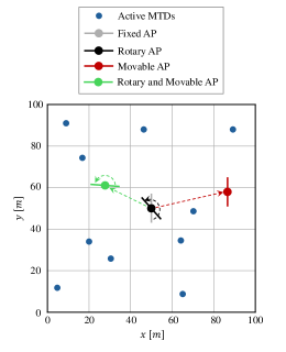
Figure 1: Illustration of the system model and the four types of APs considered in this work, for $L_{A}=100$ m and $K=10$.

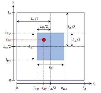
Figure 2: Illustration of the movement area of the movable APs (blue square). The red dot represents the position of the movable AP.

This paper is organized as follows. Section II presents the system and signal models, the proposed framework, the adopted performance metric and a mathematical model for the localization error. Section III introduces the mechanism for the optimization of the angular position of the rotary ULAs and the proposed location-based beamforming method to compute the objective function. Section IV presents and discusses the numerical results. Finally, Section V concludes the paper.

Notation: lowercase bold face letters denote column vectors, while boldface upper case letters denote matrices. $a_{i}$ is the $i$-th element of the column vector a, while $\textbf{a}_{i}$ is the $i$-th column of the matrix A. $\textbf{I}_{M}$ is the identity matrix with size $M\times M$. The superscripts $(\cdot)^{T}$ and $(\cdot)^{H}$ denote the transpose and the conjugate transpose of a vector or matrix, respectively. The magnitude of a scalar quantity or the cardinality of a set are denoted by $|\cdot|$. The Euclidean norm of a vector (2-norm) is denoted by $\|\cdot\rVert$. We denote the one dimensional uniform distribution with bounds $a$ and $b$ by $\mathcal{U}(a,b)$. We denote the multivariate Gaussian distribution with mean $\mathbf{a}$ and covariance $\mathbf{B}$ by $\mathcal{N}(\mathbf{a},\mathbf{B})$.

II System Model

We consider an indoor of a building. square coverage area with dimensions $L_{A}\times L_{A}\;\text{m}^{2}$. The coverage area is served by a single Access Point (AP) equipped with a Uniform Linear Array (ULA) of $M$ half-wavelength spaced antenna elements, and placed at height $h_{\text{AP}}$. The default/initial position of the AP is at the center of the coverage area, i.e., $\textbf{p}_{\text{AP}}^{0}=(x_{\text{AP}}^{0},y_{\text{AP}}^{0})=(L_{A}/2,L_{A}/2)$.

The AP serves $K$ active MTDs simultaneously. Let $\textbf{p}_{k}=(x_{k},y_{k})^{T}$ denote the coordinates of the $k$-th device, assuming for simplicity that all devices are located at the same height $h_{\text{device}}$ [17, 18].

In this work, we compare the performance of four different types of APs:

1. Fixed AP: the AP has no movement capabilities.

2. Rotary AP: the AP is able to rotate.

3. Movable AP: the AP is able to move on the $(x,y)$ directions.

4. Rotary and Movable AP: the AP can both rotate and move across the horizontal plane.

The system model is illustrated in Figure 2. The movable APs are able to move within a square area with dimensions $L_{B}\times L_{B}$ that is inscribed on the square coverage area, as illustrated in Fig. 2. Finally, Fig. 3 shows illustrations of the rotary and movable AP systems. Note that the rotary AP is equipped with a single servo motor, while the movable AP has two servo motors, cables and slide tracks.

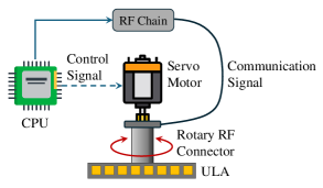
(a)

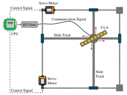
(b)

Figure 3: Illustration of (a) Rotary AP and (b) Movable AP systems [9]. The APs are equipped with a ULA of $M=8$ antenna elements.

II-A Channel Model

We adopt a spatially correlated Rician fading channel model [19]. Let $\textbf{h}_{k}\in\mathbb{C}^{M\times 1}$ denote the channel vector between the $k$-th device and the AP. It can be modeled as [20]

$$\textbf{h}_{k}=\sqrt{\dfrac{\kappa}{1+\kappa}}\textbf{h}_{k}^{\text{los}}+\sqrt{\dfrac{1}{1+\kappa}}\textbf{h}_{k}^{\text{nlos}},$$ (1)

where $\kappa$ is the Rician factor, $\textbf{h}_{k}^{\text{los}}\in\mathbb{C}^{M\times 1}$ is the deterministic LoS component, and $\textbf{h}_{k}^{\text{nlos}}\in\mathbb{C}^{M\times 1}$ is the random NLoS component.

The deterministic LoS component is given by

$$\textbf{h}_{k}^{\text{los}}=\sqrt{\beta_{k}}\begin{bmatrix}1\\ \exp(-j2\pi\Delta\sin(\phi_{k}))\\ \exp(-j4\pi\Delta\sin(\phi_{k}))\\ \vdots\\ \exp(-j2\pi(S-1)\Delta\sin(\phi_{k}))\\ \end{bmatrix},$$ (2)

where $\beta_{k}$ is the power attenuation due to the distance between the $k$-th device and the AP, $\Delta$ is the normalized inter-antenna spacing, and $\phi_{k}\in[0,2\pi]$ is the azimuth angle relative to the boresight of the ULA of the AP. Meanwhile, the random NLoS component is distributed as

$$\textbf{h}_{k}^{\text{nlos}}\sim\mathcal{CN}(\textbf{0},\textbf{R}_{k}).$$ (3)

Note that

$$\textbf{h}_{k}\sim\mathcal{CN}\left(\sqrt{\dfrac{\kappa}{1+\kappa}}\textbf{h}_{k}^{\text{los}},\dfrac{\textbf{R}_{k}}{\kappa+1}\right),$$ (4)

where $\textbf{R}_{k}\in\mathbb{C}^{M\times M}$ with $\text{Tr}(\textbf{R}_{k})=\beta_{k}$ is the positive semi-definite covariance matrix describing the spatial correlation of the NLoS components.

The spatial covariance matrices can be (approximately) modeled using the Gaussian local scattering model [21, Sec. 2.6]. Specifically, the $s$-th row, $m$-th column element of the correlation matrix is

$$\begin{split}[\textbf{R}_{k}]_{s,m}=\dfrac{\beta_{k}}{N}\sum_{n=1}^{N}\exp[j\pi(s-m)\sin(\psi_{k,n})]\\ \times\exp\left\{-\dfrac{\sigma_{\phi}^{2}}{2}[\pi(s-m)\cos(\psi_{k,n})]^{2}\right\},\end{split}$$ (5)

where $N$ is the number of scattering clusters, $\psi_{k,n}$ is the nominal Angle of Arrival (AoA) for the $n$-th cluster, and $\sigma_{\psi}$ is the Angular Standard Deviation (ASD).

To take advantage of its multiple antennas, the AP needs to estimate the channel responses from the MTDs that are active. The channel estimation is often done using pilot sequences that the UEs transmit in the uplink and are known by the AP [21]. In practice, the channel estimates are not perfect, i.e., there is a channel estimation error associated to them. The estimated channel vector of the $k$-th device, $\hat{\textbf{h}}_{k}\in\mathbb{C}^{M\times 1}$, can be modeled as the sum of the true channel vector plus a random error vector as [22, 23, 24]

$$\hat{\textbf{h}}_{k}=\textbf{h}_{k}+\tilde{\textbf{h}}_{k},$$ (6)

where $\tilde{\textbf{h}}_{k}\sim\mathcal{CN}(\textbf{0},\sigma_{\text{csi}}^{2}\textbf{I})$ is the vector of channel estimation errors. Note that the true channel realizations and the channel estimation errors are uncorrelated.

The parameter $\sigma_{\text{csi}}^{2}$ indicates the quality of the channel estimates. Let

$$\rho=\dfrac{p}{\sigma_{n}^{2}},$$ (7)

denote the per-AP antenna transmit SNR, where $p\geq 0$ is the fixed uplink transmit power (which is the same for all the devices) and $\sigma_{n}^{2}$ is the receive noise power at the APs. We assume there are $\tau_{p}$ orthogonal pilot sequences during the uplink data transmission phase, such that $\tau_{p}\geq K$. We also assume that the duration of the uplink pilot transmission phase is equal to $\tau_{p}$ symbols. Then, variance of the channel estimation errors can be modeled as a decreasing function of $\rho$ as [22, 23, 24]

$$\sigma_{\text{csi}}^{2}=\dfrac{1}{\tau_{p}\rho}.$$ (8)

Note that the channel estimation error depends only on the uplink transmit power, receive noise power and number of orthogonal pilots, thus it is the same for all devices.

II-B Signal Model

The matrix $\textbf{H}\in\mathbb{C}^{M\times K}$ containing the channel vectors of the $K$ devices transmitting their data to the AP can be written as

$$\textbf{H}=[\textbf{h}_{1},\textbf{h}_{2},\ldots,\textbf{h}_{K}].$$ (9)

Then, the $M\times 1$ received signal vector can be written as

$$\textbf{y}=\sqrt{p}\textbf{H}\textbf{x}+\textbf{n},$$ (10)

where $\textbf{x}\in\mathbb{C}^{K\times 1}$ is the vector of symbols simultaneously transmitted by the $K$ devices, and $\textbf{n}\in\mathbb{C}^{M\times 1}$ is the vector of additive white Gaussian noise samples such that $\textbf{n}\sim\mathcal{CN}(\textbf{0}_{M\times 1},\sigma^{2}_{n}\textbf{I}_{M})$.

Let $\textbf{V}\in\mathbb{C}^{M\times K}$ be a linear detector matrix used for the joint decoding of the signals transmitted from the $K$ devices. The received signal after the linear detection operation is split to $K$ streams and given by

$$\textbf{r}=\textbf{V}^{H}\textbf{y}=\sqrt{p}\textbf{V}^{H}\textbf{H}\textbf{x}+\textbf{V}^{H}\textbf{n}.$$ (11)

Let $r_{k}$ and $x_{k}$ denote the $k$-th elements of r and x, respectively. Then, the received signal corresponding to the $k$-th device can be written as

$$r_{k}=\underbrace{\sqrt{p}\textbf{v}_{k}^{H}\textbf{h}_{k}x_{k}}_{\text{Desired signal}}+\underbrace{\sqrt{p}\textbf{v}_{k}^{H}\sum_{k^{\prime}\neq k}^{K}\textbf{h}_{k^{\prime}}x_{k^{\prime}}}_{\text{Inter-user interference}}+\underbrace{\textbf{v}_{k}^{H}\textbf{n}}_{\text{Noise}},$$ (12)

where $\textbf{v}_{k}$ and $\textbf{h}_{k}$ are the $k$-th columns of the matrices V and H, respectively. From (12), the signal-to-interference-plus-noise ratio of the uplink transmission from the $k$-th device is given by

$$\gamma_{k}=\dfrac{p|\textbf{v}_{k}^{H}\textbf{h}_{k}|^{2}}{p\sum_{k^{\prime}\neq k}^{K}|\textbf{v}_{k}^{H}\textbf{h}_{k^{\prime}}|^{2}+\sigma^{2}_{n}\lVert\textbf{v}_{k}^{H}\rVert^{2}}.$$ (13)

The receive combining matrix V is computed as a function of the matrix of estimated channel vectors $\hat{\textbf{H}}\in\mathbb{C}^{M\times K}$, $\hat{\textbf{H}}=[\hat{\textbf{h}}_{1},\ldots,\hat{\textbf{h}}_{K}]$. In this work, we adopt Zero Forcing (ZF) combining. The receive combining matrix is computed as [26]

$$\textbf{V}=\hat{\textbf{H}}(\hat{\textbf{H}}^{H}\hat{\textbf{H}})^{-1}.$$ (14)

II-C Proposed Framework

In this subsection, we describe our proposed framework for the optimization of the rotation and/or position of the AP and uplink data transmission. Inspired by the three-phase scheduled random access scheme from [27], our framework has the following phases:

1. Active MTDs, i.e., MTDs seeking to send data to the network, transmit non-orthogonal uplink pilots for activity detection.

2. The AP identifies the set of active MTDs and, utilizing some indoor localization techniques, obtains estimates of the locations of the active MTDs.

3. The AP assumes pure LoS propagation and utilizes the estimated locations of the MTDs and location based beamforming to compute its optimal rotation and/or position.

4. The AP broadcasts a common downlink feedback message to assign each user an orthogonal pilot sequence.

5. The MTDs transmit their orthogonal pilot sequences and data during multiple time slots. The uplink orthogonal pilots are used to compute the CSI estimates shown in (6) for each coherence time interval, which are then used to compute the ZF receive combining vectors in (14).

The proposed framework is illustrated in Fig. 4. Note that phase 5 extends over $T$ time slots. Within each time slot, the $K$ active devices transmit simultaneously. Each time slot is as long as the channel’s coherence time interval and contains $\tau_{c}$ symbols. The first $\tau_{p}$ symbols of each time slot are used for the transmission of the orthogonal pilot sequences, while the remaining $\tau_{d}=\tau_{c}-\tau_{p}$ symbols are utilized for uplink data transmission. The numerical results presented in this work, that is, the mean per-user achievable SE presented in Section II-D, correspond to the uplink communication performance achieved in the data transmission.

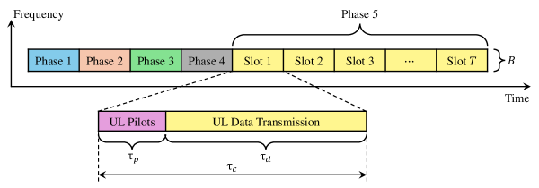
Figure 4: Illustration of the proposed framework for optimization of the rotation and/or position of the AP and uplink data transmission.

II-D Performance Metrics

We adopt as the performance metric the per-user mean achievable uplink Spectral Efficiency (SE). The achievable uplink SE of the $k$-th device is [26]

$$R_{k}=\dfrac{\tau_{d}}{\tau_{c}}\mathbb{E}_{\textbf{H}}\{\log_{2}(1+\gamma_{k})\}.$$ (15)

Then, the per-user mean achievable uplink SE is obtained by averaging over the achievable uplink SE of the $K$ devices, i.e.,

$$\bar{R}=\dfrac{1}{K}\sum_{k=1}^{K}R_{k}.$$ (16)

II-E Localization Error Model

We adopt the same localization error model that was utilized in our previous work [16]. Considering that all the devices are at the same height $h_{\text{device}}$, the imperfect positioning impairment refers to the uncertainty on the location of the devices only on the $(x,y)$ directions. Let $\textbf{p}_{k}=(x_{k},y_{k})$ denote the true location of the $k$-th device, and $\hat{\textbf{p}}_{k}=(\hat{x}_{k},\hat{y}_{k})$ denote the estimated location. The localization error vector associated to the $k$-th device can be modeled as

$$\textbf{e}_{k}=\textbf{p}_{k}-\hat{\textbf{p}}_{k}=(x_{e,k},y_{e,k}),$$ (17)

where

$$x_{e,k}=x_{k}-\hat{x}_{k},$$ (18)

$$y_{e,k}=y_{k}-\hat{y}_{k}$$ (19)

are the $x$ and $y$ components of the localization error vector, respectively.

Aiming at generality (that is, in order to not introduce any additional assumption or bias related to indoor localization in our system model), we model the localization error as a bivariate Gaussian distribution, since it is the least informative distribution for any given variance [28]. The localization error has mean $\bm{\mu}=[\textbf{0}\;\textbf{0}]^{T}$ and covariance matrix $\bm{\Sigma}=\sigma_{e}^{2}\textbf{I}_{2}$ [29]. Then, the $x$ and $y$ components of the localization error vector follow a Normal distribution:

$$x_{e,k},y_{e,k}\sim\mathcal{N}(0,\sigma_{e}^{2}).$$ (20)

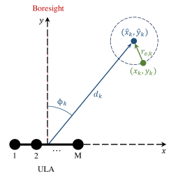
(a)

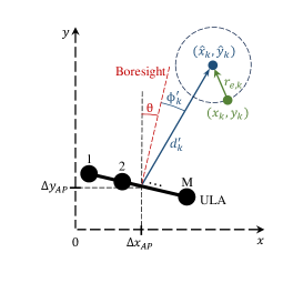
(b)

Figure 5: Illustration of the ULA of an AP and its position and rotation with respect to one active MTD (a) before movements (b) after movements. The green circle represents the true location of the device, and the blue circle represents the estimated location.

III Optimization of the Position and Rotation

In each time slot, $K$ distinct devices are active. For each subset of $K$ locations of active devices, there is a distinct optimal rotation and/or optimal position for the AP.

Let $(x_{\text{AP}}^{0},y_{\text{AP}}^{0})$ denote the initial position of the AP, and let $\theta\in[0,\pi]$ denote its rotation. The AP and its position with respect to an active MTD, before and after its movement and rotation, is illustrated in Fig. 5. The position of the AP after its movement can be written as

$$x_{\text{AP}}^{\prime}:=x_{\text{AP}}^{0}+\Delta x_{\text{AP}},$$ (21)

$$y_{\text{AP}}^{\prime}:=y_{\text{AP}}^{0}+\Delta y_{\text{AP}}.$$ (22)

The angle between the $k$-th device and the AP after the rotation of the AP is given by

$$\phi_{k}^{\prime}:=\phi_{k}+\theta.$$ (23)

These three variables can be jointly optimized. The optimization problem can be written as

maximize $$f(x_{\text{AP}},y_{\text{AP}},\theta\;|\;\hat{\textbf{p}}_{k},\forall k)$$ (24)

subject to $$l_{B}\leq x_{\text{AP}},y_{\text{AP}}\leq u_{B},$$

$$0\leq\theta\leq\pi,$$

where $f(\cdot)$ is the objective function to be maximized, and $l_{B}$ and $u_{B}$ are, the lower and upper bounds, respectively, for the movements of the AP in both $x$ and $y$ directions. The mechanism utilized to obtain the objective function is described in Section III-A. Considering that the movable APs can move only within a square with dimensions $L_{B}\times L_{B}$, inscribed on the square coverage area with dimensions $L_{A}\times L_{A}$, the lower and upper bounds for both $x_{\text{AP}},y_{\text{AP}}$ are respectively given by

$$l_{B}=\dfrac{L_{A}-L_{B}}{2},$$ (25)

$$u_{B}=\dfrac{L_{A}+L_{B}}{2}.$$ (26)

III-A Location-Based Beamforming

In this subsection, we present the mechanism utilized to compute the objective function $f(\cdot)$, which is maximized using PSO. Given the estimates of the locations of all active MTDs, that is, $\hat{\textbf{p}}_{k},\;\forall k$, we adopt a location-based beamforming [30, 31, 32, 33] approach to determine $f(\cdot)$ as a function of the position and rotation of the AP.

Based on $\hat{\textbf{p}}_{k},\;\forall k$, the AP computes the estimates for the distances and azimuth angles between the AP and the MTDs, i.e. $\hat{d}_{k}$ and $\hat{\phi}_{k}$, $\forall k$. Then, it computes pseudo channel vectors assuming pure LoS propagation as

$$\textbf{h}_{k}^{\text{pseudo}}=\sqrt{\hat{\beta}_{k}}\begin{bmatrix}1\\ \exp(-j2\pi\Delta\sin(\hat{\phi}_{k}))\\ \exp(-j4\pi\Delta\sin(\hat{\phi}_{k}))\\ \vdots\\ \exp(-j2\pi(S-1)\Delta\sin(\hat{\phi}_{k}))\\ \end{bmatrix}.$$ (27)

Note that the estimated large-scale fading coefficient $\hat{\beta}_{k}$ is computed as a function of the estimated distances $\hat{d}_{k}$ assuming a known channel model. Receive combining vectors are then computed as a function of the pseudo channel vectors according to (14). Finally, the objective function is obtained by computing the predicted mean-per user achievable SE utilizing the pseudo-channel vectors from (27) and the corresponding receive combining vectors in (13), (15) and (16). The objective function corresponds to the predicted mean per-user achievable SE, which is predicted assuming assuming full LoS propagation, versus the rotation and/movement of the AP.

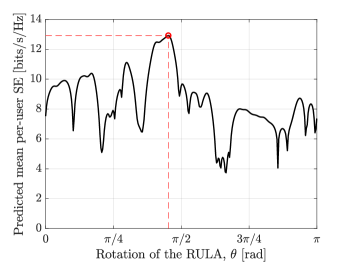
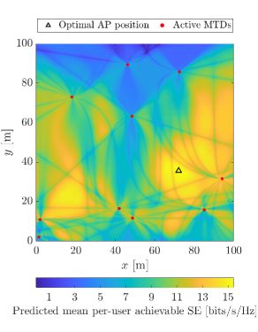
Figure 6: Objective function of the rotary AP, for $L_{A}=100$ m, $M=16$, and $K=10$.

Figure 7: Objective function of the movable AP, for $L_{A}=L_{B}=100$ m, $M=16$, and $K=10$.

Considering a single network realization, i.e., a single set of locations of $K$ active MTDS, we numerically evaluate the objective functions to be optimized. In Fig. 7, we show the objective function for the case of a rotary AP, which is the predicted mean per-user achievable SE versus the rotation of the AP. Moreover, Fig. 7 shows the objective function for the case of a movable AP, which is the predicted mean per-user achievable SE for all the points of the square coverage area. Note that both objective functions present several local minimum and maximum points. Thus, it is not possible to obtain the optimal points utilizing, for instance, convex optimization techniques [34]. For this reason, in order to obtain the optimal rotation and/or position of the AP, we employ Particle Swarm Optimization (PSO), which will be presented in the next subsection.

III-B Particle Swarm Optimization

PSO [35, Ch. 16] is an optimization algorithm highly effective for tackling problems where discovering the global maximum or minimum of a function is challenging. This algorithm operates with a population of candidate solutions, referred to as agents or particles, which are moved within the search space based on their current positions and velocities. Each particle’s trajectory is influenced by its own best-known position, as well as the global best-known position in the search space. These local and global best positions are updated with each iteration, aiming to direct the swarm of particles towards the optimal solution.

The PSO was first introduced in [36], designed to simulate social behaviors such as the motion in bird flocks or fish schools. It has been applied to a variety of optimization problems in communication systems, such as optimal deployment, node localization, clustering, and data aggregation in wireless sensor networks [37]. Additionally, it has been utilized in antenna design to achieve a specific side-lobe level or to determine the positions of antenna elements in a non-uniform array. In communication systems, it has also proven useful in computing the optimal precoding vector to maximize the throughput of a multi-user MIMO system [38], optimizing scheduling in the downlink of multi-user MIMO systems [39], and initializing channel estimates for MIMO-OFDM receivers that simultaneously perform channel estimation and decoding [40].

The parameters of the PSO algorithm are listed in Table I. Moreover, a pseudo-code for the PSO algorithm is listed in Algorithm 1. The inertial weight $w$ controls the particle’s tendency to continue in its current direction. Parameters $c_{1}$ and $c_{2}$ are the acceleration coefficients, and controls the influence of the personal and global best positions, respectively. The termination criterion might be a pre-determined maximum number of iterations, a certain threshold of the objective function $f(\cdot)$, or any other criteria related to the optimization problem.

TABLE I: Parameters of the PSO Algorithm

Symbol	Parameter
$f(\cdot)$	Objective function
$x_{i}$	Position of the $i$-th particle
$v_{i}$	Velocity of the $i$-th particle
$w$	Inertial weight
$c_{1}$	Cognitive constant
$r_{1},r_{2}$	Random numbers between 0 and 1
$c_{2}$	Social constant
$p_{b,i}$	Personal best of the $i$-th particle
$g_{b}$	Global best

Algorithm 1 Particle Swarm Optimization for $x$, $y$, and $\theta$

1:Initialize swarm:

2:for each particle $i$ in the swarm do

3:     Initialize position $\textbf{p}_{i}=(x_{i},y_{i},\theta_{i})$ randomly

4:     Initialize velocity $\textbf{v}_{i}=(v_{x_{i}},v_{y_{i}},v_{\theta_{i}})$ randomly

5:     Initialize personal best position $\textbf{p}_{b,i}=(x_{b,i},y_{b,i},\theta_{b,i})$ to the initial position

6:end for

7:Initialize global best position $\textbf{g}_{b}=(x_{gb},y_{gb},\theta_{gb})$ to the best initial particle position

8:while Stopping criterion is not met do

9:     for each particle $i$ in the swarm do

10:         for each dimension $(x,y,\theta)$ do

11:              Update velocity:

12:              $v_{x_{i}}=wv_{x_{i}}+c_{1}r_{1}(x_{b,i}-x_{i})+c_{2}r_{2}(x_{gb}-x_{i})$

13:              $v_{y_{i}}=wv_{y_{i}}+c_{1}r_{1}(y_{b,i}-y_{i})+c_{2}r_{2}(y_{gb}-y_{i})$

14:              $v_{\theta_{i}}=wv_{\theta_{i}}+c_{1}r_{1}(\theta_{b,i}-\theta_{i})+c_{2}r_{2}(\theta_{gb}-\theta_{i})$

15:         end for

16:         Update position:

17:         $x_{i}=x_{i}+v_{x_{i}}$

18:         $y_{i}=y_{i}+v_{y_{i}}$

19:         $\theta_{i}=\theta_{i}+v_{\theta_{i}}$

20:         if $f$($\textbf{p}_{i}$) is better than $f$($\textbf{p}_{b,i}$) then

21:              Update personal best: $\textbf{p}_{b,i}=(x_{i},y_{i},\theta_{i})$

22:              if $f$($\textbf{p}_{b,i}$) is better than $f$($\textbf{g}_{b})$ then

23:                  Update global best: $\textbf{g}_{b}=(x_{b,i},y_{b,i},\theta_{b,i})$

24:              end if

25:         end if

26:     end for

27:end while

28:return global best position $\textbf{g}_{b}=(x_{gb},y_{gb},\theta_{gb})$

IV Numerical Results

In this section, we present Monte Carlo simulation results to compare the performance achieved by the four different types of APs studied in this work.

IV-A Simulation Parameters

The power attenuation due to the distance (in dB) is modelled using the log-distance path loss model as

$$\beta_{k}=-L_{0}-10\eta\log_{10}\left(\dfrac{d_{k}}{d_{0}}\right),$$ (28)

where $d_{0}$ is the reference distance in meters, $L_{0}$ is the attenuation owing to the distance at the reference distance (in dB), $\eta$ is the path loss exponent and $d_{k}$ is the distance between the $k$-th device and the AP in meters. The attenuation at the reference distance is calculated using the Friis free-space path loss model and given by

$$L_{0}=20\log_{10}\left(\dfrac{4\pi d_{0}}{\lambda}\right),$$ (29)

where $\lambda=c/f_{c}$ is the wavelength in meters, $c$ is the speed of light and $f_{c}$ is the carrier frequency, as already defined in ².

Unless stated otherwise, the values of the simulation parameters adopted in this work are listed in Table III. We assume far-field propagation conditions between all the APs and all the MTDs (please refer to Appendix A). Moreover, the adopted parameters for the PSO algorithm are listed in Table III. Considering the selected values of $M$ and $h_{\text{AP}}$, the communication links between the AP and any device experience far-field propagation conditions.

The noise power (in Watts) is given by $\sigma^{2}_{n}=N_{0}BN_{F}$, where $N_{0}$ is the power spectral density of the thermal noise in W/Hz, $B$ is the signal bandwidth in Hz, and $N_{F}$ is the noise figure at the receivers. For the computation of the correlation matrices $\textbf{R}_{k},\;\forall k$, we consider $N=6$ scattering clusters, $\psi_{k,n}\sim\mathcal{U}[\phi_{k}-40\degree,\phi_{k}+40\degree]$, and $\sigma_{\psi}=5\degree$ [19].

TABLE II: Simulation parameters [17, 19, 41].

Parameter	Symbol	Value
Total number of antenna elements	$M$	16
Number of active MTDs	$K$	$10$
Length of the side of the square area	$L_{A}$	$100$ m
Uplink transmission power	$p$	100 mW
PSD of the noise	$N_{0}$	$4\times 10^{-21}$ W/Hz
Signal bandwidth	$B$	20 MHz
Noise figure	$N_{F}$	9 dB
Length of the pilot sequences	$\tau_{p}$	10 samples
Length of the time slot	$\tau_{p}$	200 samples
Height of the APs	$h_{\text{AP}}$	12 m
Height of the UEs	$h_{\text{UE}}$	1.5 m
Carrier frequency	$f_{c}$	$3.5$ GHz
Normalized inter-antenna spacing	$\Delta$	$0.5$
Path loss exponent	$\eta$	$2$
Reference distance	$d_{0}$	$1$ m

TABLE III: Parameters of the PSO Algorithm [42].

Symbol	Parameter	Value
$w$	Inertial weight	$[0.1,1.1]$
$c_{1}$	Cognitive constant	$1.49$
$c_{2}$	Social constant	$1.49$
$N_{\text{vars}}$	Number of variables	$[1,2,3]$
$|\mathcal{A}|$	Swarm size	$\min\{100,10N_{\text{vars}}\}$
$N_{\text{max}}$	Maximum number of iterations	$200N_{\text{vars}}$
$N_{\text{stall}}$	Maximum number of stall iterations	20
$\epsilon$	Function tolerance	$10^{-6}$

IV-B Simulation Results and Discussions

The locations of the devices are uniformly randomly generated in the coverage area, i.e., $x_{k},y_{k}\sim\mathcal{U}[0,L_{A}]$. We generate average performance results for networks of $K$ devices by averaging the per-user mean achievable SE over multiple network realizations. In other words, the numerical results correspond to the expected SE performance gains for networks of $K$ devices in the considered setup. For each network realization, the achievable SE of the $K$ devices is obtained by averaging over several channel realizations, i.e. distinct realizations of the channel matrix H. In the case of movable APs, we evaluate the performance achieved with different sizes of the movement area, i.e., different values of $L_{B}$. Note that, in practice, the movement area of the movable APs cannot be very large owing to size and costs constraints. Moreover, moving an AP over long distances might take a considerable amount of time (which can be longer than the coherence time of the wireless channel), even when high-speed servo motors are utilized. Thus, the numerical results for the case of $L_{B}=L_{A}=100$ m, that is, when the movement area covers the whole coverage area, are hypothetical results that represent an ideal scenario and are utilized here solely for benchmark purposes.

Fig. 11 shows the mean per-user achievable SE versus the Rician factor. In the case of an AP equipped with a static antenna array or a movable AP with a very constrained movement area, we observe that the achievable SE decreases with the Rician factor, while it increases with $\kappa$ when we adopt a rotary AP or a movable AP with a large movement area. Note that the performance gains obtained with the optimal rotations or movements become very significant when the LoS component is very strong. As expected, the best performance is achieved with the movable and rotary AP, since it has three degrees of freedom for the movements. However, it features the most complex and expensive setup. The movable AP, which has two degrees of freedom for the movement, outperforms the rotary AP only when the movement area covers the whole coverage area. It is very interesting to observe that the rotary AP outperforms the movable AP in the case of $L_{B}=25$ m, which corresponds to a very large movement area.

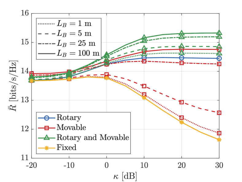
Figure 8: Mean per-user achievable SE versus the Rician factor $\kappa$, for $\sigma_{e}^{2}=-10$ dB.

Figure 9: Mean per-user achievable SE versus dimensions of the movement area, for $\kappa=10$ dB and $\sigma_{e}^{2}=-10$ dB.

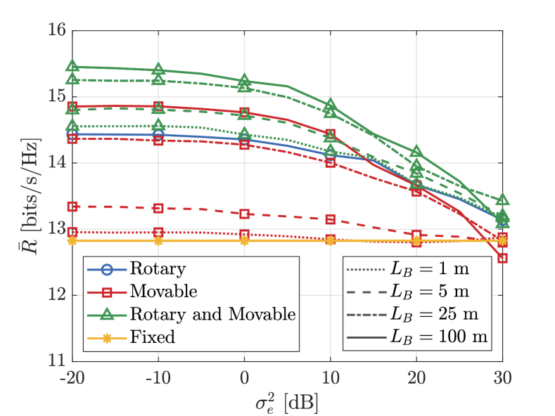
Figure 10: Mean per-user achievable SE versus variance of the localization error considering $\kappa=10$ dB.

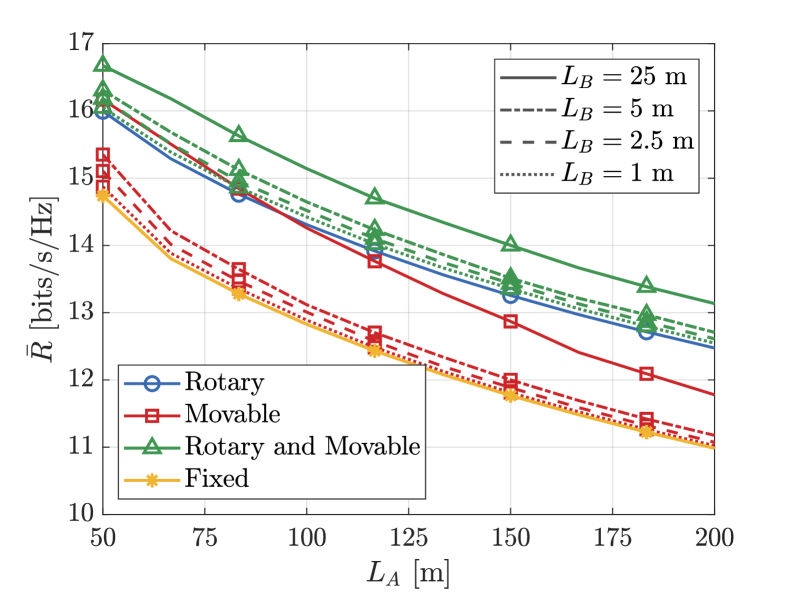
Figure 11: Mean per-user achievable SE versus dimensions of the coverage area, for $\kappa=10$ dB and $\sigma_{e}^{2}=-10$ dB.

Fig. 11 shows the mean per-user achievable SE versus the dimensions of the movement area for $\kappa=10$ dB, i.e., a situation where the LoS component of the channel vectors is very strong. When $L_{B}\rightarrow 0$ m, the performance obtained with the movable AP converges to the performance obtained with the static one, while the performance obtained with the rotary and movable AP converges to the performance obtained with the rotary AP, as expected. As we increase the size of the movement area, the performance gains obtained with the movement of the antenna array becomes noticeable. We observe again that the rotary and movable AP always presents the best performance. When adopting the movable AP, we need a considerably large movement area ($L_{B}>25$ m) in order to achieve the same performance that can be obtained by simply rotating the antenna array. Note also that the performance improvement obtained by increasing the size of the movement area is negligible for $L_{B}\geq 50$ m.

Fig. 11 shows the mean per-user achievable SE versus the variance of the localization error. We observe that all the optimal rotations and movements of the APs bring noticeable performance improvements even when the accuracy of the localization information is poor. However, the performance gains on the achievable SE when compared to the case of a fixed AP decay rapidly for $\sigma_{e}^{2}\geq 10$ dB. We again observe that the best performance is achieved by the movable and rotary AP, followed by the movable AP and then the rotary AP. Nevertheless, note that increasing the accuracy of the localization information to sub-cm or mm levels do not yield performance improvements.

Finally, Fig. 11 shows the mean per-user achievable SE versus the dimensions of the coverage area, for $M=16$ and $K=10$. As expected, the achievable SE decreases with $L_{A}$ for any of the considered setups due to the increased path-losses. We also observe that rotating and/or moving the AP always improves the mean per-user achievable SE compared to the case of a fixed AP. Nonetheless, when the movement area is very constrained, specifically $L_{B}=1$ m, the performance improvement obtained by moving the AP on the horizontal plane is very small. Therefore, a larger movement area is essential to achieve substantial improvements in spectral efficiency. It is noteworthy that the rotary AP always outperforms the movable APs with $L_{B}=\{1,2.5,5\}$ m, and it can even outperform the movable AP with $L_{B}=25$ m when $L_{A}>95$ m, which corresponds to a setup with a large movement area. This finding demonstrates that rotating the AP provides greater improvements in the mean per-user achievable SE compared to moving the AP along the horizontal plane, even when the movement area on the horizontal plane is relatively large. Finally, note that the best performance is always achieved by the rotary and movable AP, which has more degrees of freedom at the cost of the most complex setup.

Overall, the optimal movements and rotations of the APs bring substantial improvements in the mean per-user achievable SE when the LoS components of the channel vectors is strong. When the movement area is not constrained, the best performance is achieved by the movable and rotary AP (which has three degrees of freedom for movement), followed by the movable AP (two degrees of freedom) and then by the rotary AP (one degree of freedom). Nevertheless, the movements of the APs on the $(x,y)$ directions need to be constrained in practice due to size, costs, complexity and latency limitations. Moving the AP along large distances might induce very high latency. When the movements of the APs are constrained, the rotary APs outperforms them, while simultaneously presenting a significantly lower size, complexity, and deployment and maintenance costs.

V Conclusions

In this work, we compared the performance of movable APs, which are able to move on the horizontal plane using two servo motors, cables and slide tracks, with rotary APs, which are APs simply equipped a single servo motor that can rotate on its own axis. We also proposed the combination of both schemes into movable and rotary APs, which are APs that can move on the horizontal plane and also rotate. The optimal position and/or rotation of the APs is computed based on estimates of the locations of the active MTDs and using PSO. Our numerical results show that the movable APs outperform the rotary APs when their movement area is large enough, but at the cost of a bulkier setup with higher maintenance and deployment costs. When the movement area of the APs is constrained, the rotary APs perform better and also correspond to a simpler and cheaper system. All the proposed techniques offer significant performance gains in terms of mean per-user achievable SE when compared to static APs when the LoS component of the channel vectors is strong, and all the schemes are robust against imperfect location estimates.

Appendix A Far-Field Propagation Conditions

The Fraunhofer distance determines the threshold between the near-field and far-field propagation, and is given by $d_{F}=2D^{2}/\lambda$ [43], where $D$ is the largest dimension of the antenna array, $\lambda=c/f_{c}$ is the wavelength, $c$ is the speed of the light and $f_{c}$ is the carrier frequency. In the case of an ULA with $M$ antenna elements spaced by half-wavelength, the length of the ULA is $D_{\text{ULA}}=(M-1)\lambda/2$.

Considering that a device can be located right bellow an AP in an indoor setting, the minimum height of the AP required to ensure far-field propagation conditions for all the devices is given by

$$\begin{split}h_{\text{AP}}^{\text{min}}&=d_{F}+h_{\text{device}}\\ &=\dfrac{2}{\lambda}\left((M-1)\dfrac{\lambda}{2}\right)^{2}+h_{\text{device}}\\ &=\dfrac{\lambda}{2}(M-1)^{2}+h_{\text{device}}.\end{split}$$ (30)

Considering $f_{c}=3.5$ GHz, $M=16$, $h_{\text{device}}=1.5$ m, we obtain $D_{\text{ULA}}=0.64$ m and $d_{F}=9.64$ m. Thus, the minimum height of the APs is $h_{\text{AP}}^{\text{min}}=11.14$ m.

References

- [1] C. Lim et al., “Recent Trend of Multiuser MIMO in LTE-Advanced,” IEEE Commun. Mag., vol. 51, no. 3, pp. 127–135, 2013.
- [2] F. Boccardi et al., “Five Disruptive Technology Directions for 5G,” IEEE Commun. Mag., vol. 52, no. 2, pp. 74–80, 2014.
- [3] S. Avallone et al., “Will OFDMA Improve the Performance of 802.11 Wifi Networks?” IEEE Wireless Commun., vol. 28, no. 3, pp. 100–107, 2021.
- [4] R. W. Heath Jr and A. Lozano, Foundations of MIMO Communication. Cambridge University Press, 2018.
- [5] H. Do, N. Lee, and A. Lozano, “Reconfigurable ULAs for Line-of-Sight MIMO Transmission,” IEEE Trans. Wireless Commun., vol. 20, no. 5, pp. 2933–2947, 2021.
- [6] O. L. A. López et al., “A Low-Complexity Beamforming Design for Multiuser Wireless Energy Transfer,” IEEE Wireless Commun. Letters, vol. 10, no. 1, pp. 58–62, 2021.
- [7] ——, “CSI-Free Rotary Antenna Beamforming for Massive RF Wireless Energy Transfer,” IEEE Internet Things J., vol. 9, no. 10, pp. 7375–7387, 2022.
- [8] A. Zubow, A. Memedi, and F. Dressler, “Towards Hybrid Electronic-Mechanical Beamforming for IEEE 802.11ad,” in 18th Wireless On-Demand Netw. Syst. Serv. Conf. (WONS), 2023, pp. 88–91.
- [9] L. Zhu, W. Ma, and R. Zhang, “Movable Antennas for Wireless Communication: Opportunities and Challenges,” IEEE Commun. Mag., vol. 62, no. 6, pp. 114–120, 2024.
- [10] Z. Xiao et al., “Multiuser Communications with Movable-Antenna Base Station: Joint Antenna Positioning, Receive Combining, and Power Control,” arXiv preprint arXiv:2308.09512, 2023.
- [11] K. Lin et al., “On CSI-Free Multiantenna Schemes for Massive Wireless-Powered Underground Sensor Networks,” IEEE Internet Things J., vol. 10, no. 19, pp. 17 557–17 570, 2023.
- [12] J. Li et al., “DOA estimation with a rotational uniform linear array (RULA) and unknown spatial noise covariance,” Multidimens. Syst. Signal Process., vol. 29, pp. 537–561, 2018.
- [13] H. Wang et al., “Deployment Algorithms of Flying Base Stations: 5G and Beyond With UAVs,” IEEE Internet Things J., vol. 6, no. 6, pp. 10 009–10 027, 2019.
- [14] G. Amponis et al., “Drones in B5G/6G Networks as Flying Base Stations,” Drones, vol. 6, no. 2, p. 39, 2022.
- [15] S. A. H. Mohsan et al., “Unmanned Aerial Vehicles (UAVs): Practical Aspects, Applications, Open Challenges, Security Issues, and Future Trends,” Intell. Serv. Robot., vol. 16, no. 1, pp. 109–137, 2023.
- [16] E. N. Tominaga et al., “On the Spectral Efficiency of Indoor Wireless Networks with a Rotary Uniform Linear Array,” arXiv preprint arXiv:2402.05583, 2024.
- [17] H. Q. Ngo et al., “Cell-Free Massive MIMO Versus Small Cells,” IEEE Trans. Wireless Commun., vol. 16, no. 3, pp. 1834–1850, 2017.
- [18] Z. Chen and E. Björnson, “Channel Hardening and Favorable Propagation in Cell-Free Massive MIMO With Stochastic Geometry,” IEEE Trans. Commun., vol. 66, no. 11, pp. 5205–5219, 2018.
- [19] O. Özdogan, E. Björnson, and E. G. Larsson, “Massive MIMO With Spatially Correlated Rician Fading Channels,” IEEE Trans. Commun., vol. 67, no. 5, pp. 3234–3250, 2019.
- [20] D. Kumar et al., “Latency-Aware Joint Transmit Beamforming and Receive Power Splitting for SWIPT Systems,” in IEEE 32nd Annu. Int. Symp. Personal Indoor Mobile Radio Commun. (PIMRC), 2021, pp. 490–494.
- [21] E. Björnson et al., “Massive MIMO networks: Spectral, energy, and hardware efficiency,” Foundations and Trends® in Signal Processing, vol. 11, no. 3-4, pp. 154–655, 2017.
- [22] C. Wang, T. C.-K. Liu, and X. Dong, “Impact of Channel Estimation Error on the Performance of Amplify-and-Forward Two-Way Relaying,” IEEE Trans. Veh. Technol., vol. 61, no. 3, pp. 1197–1207, 2012.
- [23] E. Eraslan, B. Daneshrad, and C.-Y. Lou, “Performance Indicator for MIMO MMSE Receivers in the Presence of Channel Estimation Error,” IEEE Wireless Commun. Letters, vol. 2, no. 2, pp. 211–214, 2013.
- [24] O. L. A. López et al., “Massive MIMO With Radio Stripes for Indoor Wireless Energy Transfer,” IEEE Trans. Wireless Commun., vol. 21, no. 9, pp. 7088–7104, 2022.
- [25] D. Tse and P. Viswanath, Fundamentals of Wireless Communication. Cambridge University Press, 2005.
- [26] P. Liu et al., “Spectral Efficiency Analysis of Cell-Free Massive MIMO Systems With Zero-Forcing Detector,” IEEE Trans. Wireless Commun., vol. 19, no. 2, pp. 795–807, 2020.
- [27] J. Kang and W. Yu, “Scheduling Versus Contention for Massive Random Access in Massive MIMO Systems,” IEEE Trans. Commun., vol. 70, no. 9, pp. 5811–5824, 2022.
- [28] F. Gustafsson and F. Gunnarsson, “Mobile Positioning Using Wireless Networks: Possibilities and Fundamental Limitations Based on Available Wireless Network Measurements,” IEEE Signal Process. Mag., vol. 22, no. 4, pp. 41–53, 2005.
- [29] B. Zhu, Z. Zhang, and J. Cheng, “Outage Analysis and Beamwidth Optimization for Positioning-Assisted Beamforming,” IEEE Commun. Lett., vol. 26, no. 7, pp. 1543–1547, 2022.
- [30] R. Maiberger, D. Ezri, and M. Erlihson, “Location Based Beamforming,” in IEEE 26th Convention Electrical Electron. Eng. Israel, 2010, pp. 000 184–000 187.
- [31] P. Kela et al., “Location Based Beamforming in 5G Ultra-Dense Networks,” in IEEE 84th Veh. Technol. Conf. (VTC-Fall), 2016, pp. 1–7.
- [32] S. Yan and R. Malaney, “Location-Based Beamforming for Enhancing Secrecy in Rician Wiretap Channels,” IEEE Trans. Wireless Commun., vol. 15, no. 4, pp. 2780–2791, 2016.
- [33] C. Liu and R. Malaney, “Location-Based Beamforming and Physical Layer Security in Rician Wiretap Channels,” IEEE Trans. Wireless Commun., vol. 15, no. 11, pp. 7847–7857, 2016.
- [34] S. P. Boyd and L. Vandenberghe, Convex Optimization. Cambridge University Press, 2004.
- [35] A. P. Engelbrecht, Computational Intelligence: an Introduction. John Wiley & Sons, 2007.
- [36] J. Kennedy and R. Eberhart, “Particle Swarm Optimization,” in Proc. Int. Conf. Neural Networks (ICNN), vol. 4, 1995, pp. 1942–1948 vol.4.
- [37] R. V. Kulkarni and G. K. Venayagamoorthy, “Particle Swarm Optimization in Wireless-Sensor Networks: A Brief Survey,” IEEE Trans. Syst. Man Cybern. Part C (Appl. Rev.), vol. 41, no. 2, pp. 262–267, 2011.
- [38] F. Shu, W. Gang, and L. Shao-Qian, “Optimal Multiuser MIMO Linear Precoding with LMMSE Receiver,” EURASIP J. Wireless Commun. Netw., vol. 2009, pp. 1–10, 2009.
- [39] Y. Hei et al., “Novel Scheduling Strategy for Downlink Multiuser MIMO System: Particle Swarm Optimization,” Sci. China Ser. F: Inf. Sci., vol. 52, no. 12, pp. 2279–2289, 2009.
- [40] C. Knievel et al., “Particle Swarm Enhanced Graph-Based Channel Estimation for MIMO-OFDM,” in IEEE 73rd Veh. Technol. Conf. (VTC-Spring), 2011, pp. 1–5.
- [41] Nokia and Nokia Shangai Bell, “Scenarios, Frequencies and New Field Measurements Results from Two Operational Factory Halls at 3.5 GHz for Various Antenna Configurations.” Document R1-1813177, 3GPP, Sophia Antipolis, France, Nov. 2018. [Online]. Available: https://www.3gpp.org/ftp/tsg_ran/WG1_RL1/TSGR1_95/Docs/
- [42] MathWorks, Particle Swarm Optimization, 2024, Accessed: 2024-06-20. [Online]. Available: https://se.mathworks.com/help/gads/particleswarm.html
- [43] J. Sherman, “Properties of Focused Apertures in the Fresnel Region,” IRE Trans. Antennas Propag., vol. 10, no. 4, pp. 399–408, 1962.