One Year of SN 2023ixf: Breaking Through the Degenerate Parameter Space in Light-Curve Models with Pulsating Progenitors

Abstract

We present and analyze the extensive optical broadband photometry of the Type II SN 2023ixf up to one year after explosion. We find that, when compared to two pre-existing model grids, the pseudo-bolometric light curve is consistent with drastically different combinations of progenitor and explosion properties. This may be an effect of known degeneracies in Type IIP light-curve models. We independently compute a large grid of MESA+STELLA single-star progenitor and light-curve models with various zero-age main-sequence masses, mass-loss efficiencies, and convective efficiencies. Using the observed progenitor variability as an additional constraint, we select stellar models consistent with the pulsation period and explode them according to previously established scaling laws to match plateau properties. Our hydrodynamic modeling indicates that SN 2023ixf is most consistent with a moderate-energy ($E_{\rm exp}\approx 7\times 10^{50}$ erg) explosion of an initially high-mass red supergiant progenitor ($\gtrsim 17\ M_{\odot}$) that lost a significant amount of mass in its prior evolution, leaving a low-mass hydrogen envelope ($\lesssim 3\ M_{\odot}$) at the time of explosion, with a radius $\gtrsim 950\ R_{\odot}$ and a synthesized ⁵⁶Ni mass of $0.07\ M_{\odot}$. We posit that previous mass transfer in a binary system may have stripped the envelope of SN 2023ixf’s progenitor. The analysis method with pulsation period presented in this work offers a way to break degeneracies in light-curve modeling in the future, particularly with the upcoming Vera C. Rubin Observatory Legacy Survey of Space and Time, when a record of progenitor variability will be more common.

1 Introduction

Type II supernovae (SNe II) are hydrogen-rich core-collapse supernovae (CCSNe) that are thought to mark the violent deaths of massive stars ($\gtrsim 8\ M_{\odot}$; e.g., Woosley & Weaver 1986). Those with a plateau shape in the light curves (SNe IIP) are the most common variety of massive star explosion, representing about half of all CCSNe (Smith et al. 2011). Their progenitors have been confirmed to be red supergiants (RSGs) by pre-explosion detections, with zero-age main-sequence (ZAMS) masses in the range $\sim 8-20\ M_{\odot}$ (Van Dyk et al. 2003, 2012, 2023; Li et al. 2006; Smartt 2009, 2015; Davies & Beasor 2020). Even with direct detections of the progenitor star in pre-explosion imaging, inferring the initial mass of the exploding star is subject to significant uncertainty, leading to much debate about the initial masses of SNe IIP (Smartt 2015; Davies & Beasor 2018, 2020). Clues to the star’s mass may also be inferred from the shape of the plateau light curve, since this shape is mediated by the recombination of the hydrogen envelope (e.g., Popov 1993; Kasen & Woosley 2009; Dessart et al. 2013). This is complicated, however, by the fact that the light-curve shape depends on other factors like the explosion energy and progenitor radius (e.g., Martinez et al. 2022b).

Extensive photometric and spectroscopic follow-up at multiple wavelengths over the duration of SN II light curves can help probe the underlying physics during different phases of their evolution (e.g., Dessart & Hillier 2005; Hillier & Dessart 2019). In particular, when SNe II are discovered very soon after explosion, early observations offer unique insight into explosion geometry, surrounding environments, mass loss during the final years of a massive star’s life, which remains poorly understood (see, e.g., Smith 2014; Li et al. 2024).

Spectroscopic observations of some SNe II within a few days from explosion revealed narrow emission features from slow circumstellar material (CSM) with high-ionization states (Niemela et al., 1985; Garnavich & Ann, 1994; Quimby et al., 2007; Gal-Yam et al., 2014; Groh, 2014; Smith et al., 2015; Shivvers et al., 2015; Khazov et al., 2016; Yaron et al., 2017; Bullivant et al., 2018; Tartaglia et al., 2021; Bruch et al., 2021, 2023; Zhang et al., 2023; Andrews et al., 2024; Shrestha et al., 2024a, b). Combined with recent efforts of detailed hydrodynamic and radiative transfer modeling (Morozova et al. 2017, 2018; Boian & Groh 2019; Moriya et al. 2023) and a number of SNe II exhibiting light-curve excess above the canonical shock-cooling model (e.g., Hosseinzadeh et al. 2018; Andrews et al. 2019; Dong et al. 2021; Tartaglia et al. 2021; Hosseinzadeh et al. 2022; Pearson et al. 2023; Andrews et al. 2024; Shrestha et al. 2024a, b), we now see an increasing number of SN II progenitors enshrouded in dense CSM shells or inflated envelopes (e.g., Förster et al. 2018; Morozova et al. 2018; Bruch et al. 2023; Jacobson-Galán et al. 2024). If one assumes the dense CSM shell is unbound, its formation requires an enhanced mass-loss rate $\sim 10^{-4}-10^{-2}\ M_{\odot}\ {\rm yr^{-1}}$ in the months to years prior to the onset of core-collapse, which is much higher than values expected for normal stellar winds of RSGs (e.g., Mauron & Josselin 2011; Beasor & Davies 2018; Beasor et al. 2020; Beasor & Smith 2022). While the exact nature for such an intense mass-loss episode is still unclear, several mechanisms have been proposed, including, but not limited to, late-phase nuclear burning instabilities (Arnett & Meakin 2011; Smith & Arnett 2014; Woosley & Heger 2015), gravity wave driven mass loss (Quataert & Shiode 2012; Shiode et al. 2013; Shiode & Quataert 2014; Fuller 2017; Wu & Fuller 2021, 2022), binary interaction (Smith & Arnett, 2014), atmospheric shocks (Fuller & Tsuna, 2024), and pulsation-driven superwinds (Yoon & Cantiello 2010).

Recently, SN 2023ixf provided another clear case of an SN II progenitor surrounded by dense CSM structures, since it was discovered very early after explosion (Hosseinzadeh et al. 2023b; Li et al. 2024) and showed short-lived narrow emission lines in its early spectra. SN 2023ixf is a SN II (Perley et al. 2023) discovered on 2023 May 19 17:27:15.00 UT (Itagaki 2023) in the Pinwheel galaxy. Nevertheless, the earliest observation of this SN can be traced back to about 0.9 day before discovery, corresponding to a phase at about 1 hour after explosion (Li et al. 2024). Its proximity to Earth offers an unprecedented opportunity to study the late-stage evolution of RSGs and physics pertaining to SNe II encoded in its extensively sampled light curve across the electromagnetic spectrum. Analyses of both the early light curve and spectral series from radio to X-ray wavelengths all indicated the presence of dense CSM surrounding the RSG progenitor (Berger et al. 2023; Bostroem et al. 2023; Grefenstette et al. 2023; Hiramatsu et al. 2023; Jacobson-Galán et al. 2023; Matthews et al. 2023; Panjkov et al. 2023; Smith et al. 2023; Teja et al. 2023; Yamanaka et al. 2023; Zhang et al. 2023; Chandra et al. 2024). This was further supported by optical spectropolarimetry observations (Vasylyev et al. 2023; Singh et al. 2024) and evolution of shock breakout emission (Li et al. 2024), suggesting that the either the CSM or the explosion was asymmetric. The inferred mass-loss rate from these studies probed a wide range of $\sim 10^{-6}-10^{-2}\ M_{\odot}\ {\rm yr}^{-1}$ at various layer of the CSM, indicating a time-variable mass-loss history.

Using pre-explosion images from the Hubble Space Telescope, Spitzer Space Telescope, and various ground-based facilities, the properties of the candidate RSG progenitor of SN 2023ixf have also been estimated. In particular, the ZAMS mass estimated independently from spectral energy density (SED) fitting, comparison with single-star evolutionary tracks, environmental study in the vicinity of the SN, and analysis of infrared (IR) variability collectively yield a large range of $\sim 8-20\ M_{\odot}$ (Jencson et al. 2023; Niu et al. 2023; Pledger & Shara 2023; Qin et al. 2023; Soraisam et al. 2023; Van Dyk et al. 2024; Neustadt et al. 2024; Xiang et al. 2024). Given the uncertainties in both the progenitor’s inferred mass-loss rate and initial mass, it is useful to derive the progenitor properties using an alternative method. For example, Bersten et al. (2024) compared the bolometric light curve and expansion velocity evolution of SN 2023ixf to hydrodynamic models. They found a model with an initial mass of $12\ M_{\odot}$, an explosion energy of $1.2\times 10^{51}\ {\rm erg}$, and a synthesized ⁵⁶Ni mass of $0.05\ M_{\odot}$ to be compatible with the observed luminosity evolution. Similar low-mass progenitor models were also favored in Moriya & Singh (2024) and Singh et al. (2024).

In this paper, we present new observations and an independent analysis of the densely sampled optical light curves of SN 2023ixf. The optical photometry presented in this paper has a $\sim 2$ day cadence in 5 bands, extending up to a year after discovery. We give a description of the observations and the data reduction process in Section 2, followed by the methodologies used to calculate the pseudo-bolometric light curve and plateau and radioactive tail properties of SN 2023ixf. Section 3 compares our observations to publicly available hydrodynamic model grids and Section 4 presents our independent modeling of the pseudo-bolometric and multi-band light curves. We additionally include the observed RSG variability to aid model selection, and this reveals evidence for a small H-rich envelope mass and high ZAMS mass for SN 2023ixf’s progenitor. As such, we discuss the possible formation channel and implications for the progenitor of SN 2023ixf in Section 5. Finally, we summarize our findings and draw conclusions in Section 6.

2 Observations and Initial Analysis

2.1 Photometry and Reductions

Following the discovery of SN 2023ixf by Itagaki (2023), continuous photometric monitoring of the Pinwheel Galaxy was carried out using the Sinistro cameras on Las Cumbres Observatory’s robotic 1m telescopes (Brown et al. 2013) located at the Siding Spring Observatory, the South African Astronomical Observatory, and the Cerro Tololo Inter-American Observatory as part of the Global Supernova Project (GSP) collaboration (Howell & Global Supernova Project 2017). The $UBVgriz_{s}$ data were reduced using lcogtsnpipe (Valenti et al. 2016), a PyRAF-based image reduction pipeline that utilizes a standard point-spread function fitting procedure to measure instrumental magnitudes. UBV magnitudes were calibrated to stars in the L92 standard fields of Landolt (1983, 1992) observed on the same night with the same telescopes, gri magnitudes were calibrated to the AAVSO Photometric All-Sky Survey (Henden et al. 2016) catalog, and the z_s magnitudes were calibrated to the Sloan Digital Sky Survey (SDSS Collaboration 2017) catalog. The early photometry up to 2023 June 18 (MJD = 60113; 30 days after discovery) following the same reduction procedures has been presented in Hosseinzadeh et al. (2023b) and Hiramatsu et al. (2023). The reduced light curves are shown in Figure 1.

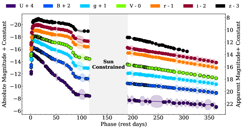
Figure 1: Optical ($UBVgriz_{s}$) light curves of SN 2023ixf from LCO, corrected for Milky Way and host extinctions. The error bars of the observed magnitudes ($\lesssim 0.1$ mag) are smaller than the marker size. The vertical region shaded in light gray indicates the duration that SN 2023ixf was unobservable. Solid colored lines are the median interpolated values and colored regions correspond to $1\sigma$ bounds from our GP interpolator for each filter. Due to gaps in data in some bands, the $1\sigma$ uncertainties returned by the GP interpolators are sometimes larger than the typical error bars associated with observations.
(The data used to create this figure are available in the published version.)

The Pinwheel Galaxy has a luminosity distance of $d_{L}=6.71\pm 0.14$ Mpc ($\mu=29.135\pm 0.045$ mag; Riess et al. 2016), measured via the Leavitt (1908) Law of Cepheid variables. The Milky Way reddening in the direction of SN 2023ixf is $E(B-V)_{\rm MW}=0.0077$ mag (Schlafly & Finkbeiner 2011), and the host-galaxy extinction is $E(B-V)_{\rm host}=0.031\pm 0.006$ mag (Lundquist et al. 2023; Smith et al. 2023). We correct for these using a Fitzpatrick (1999) extinction law with $R_{V}=3.1$ and adopt MJD 60082.788 as the explosion date, following the analysis of Li et al. (2024). $UBV$ and $griz_{s}$ magnitudes are reported in the Vega and AB systems, respectively.

2.2 Pseudo-Bolometric Light Curve

With a large set of photometric data with optical coverage ($3250-9740$ Å), we first proceed to calculate the pseudo-bolometric light curve of SN 2023ixf used for subsequent modeling purposes. We note that without additional UV photometry coverage (such as those from Swift; Hiramatsu et al. 2023; Zimmerman et al. 2024; Singh et al. 2024), the pseudo-bolometric luminosity may be underestimated by a factor of $\sim 2-10$ during the first $\approx 10$ days of SN 2023ixf’s evolution. However, as we show later in this paper, we are primarily concerned with properties on the plateau and not the initial peak, therefore our pseudo-bolometric light curve constructed with only optical coverage is sufficient (e.g., Martinez et al. 2022a, 2024). To obtain observations at all intermediate epochs, we interpolate the multi-band light curves using Gaussian processes (GPs) as done in Martinez et al. (2022a), carried out in scikit-learn (Pedregosa et al. 2011). The resulting interpolations are shown in Figure 1. In constructing the pseudo-bolometric light curve, we do not extrapolate $z$-band at early times ($t<4.4$ days) since the interpolated values for these epochs are not well-behaved owing to a lack of observed data to constrain the GP interpolators (and once again, do not contribute as much compared to UV emissions).

Equipped with photometric measurements and interpolations in all available bands at all epochs, we convert the magnitudes to monochromatic fluxes at the mean wavelength of each filter using the transmission functions and the AB magnitude zero-points. The pseudo-bolometric light curve is then calculated via full integration of the monochromatic fluxes using the trapezoidal rule within the mean wavelength range. To account for magnitude uncertainties, we perform a Monte Carlo procedure by sampling a Gaussian distribution centered at the magnitude value with the magnitude uncertainty as one standard deviation. This procedure is done 10,000 times for each epoch, and we report the median and standard deviation as the corresponding pseudo-bolometric luminosity and uncertainty for the epoch.

For later modeling purposes, we also perform blackbody fits to the SED to obtain the effective blackbody temperature and photospheric radius at day 50 using the Python-based MCMC routine emcee (Foreman-Mackey et al. 2013), implemented in the Light Curve Fitting package (Hosseinzadeh et al. 2023a). We calculate UV and IR bolometric corrections at day 50 by integrating the best-fit blackbody spectrum from zero to $U$-band and from $z$-band to infinity. The bolometric luminosity at day 50 ($L_{50}$) is then derived by summing the pseudo-bolometric luminosity with the bolometric corrections. A similar Monte Carlo procedure is performed by sampling the posterior distributions of the blackbody fits to obtain uncertainty estimates on $L_{50}$. Since SN 2023ixf has already transitioned to the photospheric phase by day 50, we regard our calculation of $L_{50}$ to be an accurate value that enables robust modeling (see Section 4.1).

We do not calculate the full bolometric light curve since we do not have complete coverage of UV and NIR photometry, which are crucial for determining bolometric corrections at early and late times, respectively. Furthermore, blackbody approximations become an inadequate description for SEDs during the nebular phase, since the spectrum for SN 2023ixf becomes mostly emission-dominated (e.g., Ferrari et al. 2024; Singh et al. 2024). For the full evolution of photospheric properties of SN 2023ixf, we refer readers to Zimmerman et al. (2024) and Singh et al. (2024).

2.3 Measuring Plateau Duration and Nickel Mass

We estimate the plateau duration $t_{p}$ following Valenti et al. (2016), fitting the functional form $y(t)=V_{\rm mag}$ to the $V$-band light curve and $y(t)=\log_{10}(L_{\rm pseudo})$ to the pseudo-bolometric light curve around the fall from the plateau:

$$y(t)=\frac{-A_{0}}{1+e^{(t-t_{p})/W_{0}}}+P_{0}\times\left(t-t_{p}\right)+M_{0}$$ (1)

We fit the light curves starting at day 60 (which corresponds to when the evolution is $\approx$75% of the way to its steepest descent; Goldberg et al. 2019) using the Python routine scipy.optimize.curve_fit, fixing $P_{0}$ to be the slope on the ⁵⁶Ni tail. The derived median and $1\sigma$ uncertainty for the plateau duration is $t_{p}=81.75^{+0.38}_{-0.38}$ days for the $V$-band light curve and $t_{p}=81.50^{+0.11}_{-0.11}$ days for the pseudo-bolometric light curve.

Curiously, the derived slope on the radioactive tail for the $V$-band light curve corresponds to a decline rate of $\approx 1.26$ mag per 100 days, higher than the value of $\approx 0.98$ mag per 100 days expected for the typical ⁵⁶Ni decay. The steepened slope during the nebular phase could be explained by incomplete trapping due to $\gamma$-ray leakage, commonly seen in short-plateau SNe IIP with steeper declines, where the progenitors have partially-stripped, low-density envelopes (e.g., Anderson et al. 2014; Morozova et al. 2015; Paxton et al. 2018; Hiramatsu et al. 2021). In accordance with the steeper decline rate, we fit the pseudo-bolometric light curve with a modified energy deposition rate from Wheeler et al. (2015):

$$L_{\rm tail}=Q_{\rm Ni}\left(1-e^{-(T_{0}/t)^{2}}\right)$$ (2)

where

$$Q_{\rm Ni}=\frac{M_{\rm Ni}}{M_{\odot}}\left(6.45e^{-t/t_{\rm Ni}}+1.45e^{-t/t_{\rm Co}}\right)\times 10^{43}\ {\rm erg\ s^{-1}}$$ (3)

is the ⁵⁶Ni$\rightarrow$⁵⁶Co$\rightarrow$⁵⁶Fe decay luminosity given by Nadyozhin (1994), $t_{\rm Ni}=8.8$, $t_{\rm Co}=111.3$ days, $t$ is the time in days since the explosion, and $T_{0}$ is the $\gamma$-ray diffusion timescale. Roughly speaking, $T_{0}$ indicates the strength of $\gamma$-ray trapping within the ejecta. As $T_{0}\rightarrow\infty$, the instantaneous heating rate given by Equation 3 is recovered and no leakage occurs (i.e., complete trapping). We note that since we are using the pseudo-bolometric light curve, the values derived here only serve as lower limits, as NIR luminosity contributes up to a factor of $\sim 2$ in the total luminosity (Singh et al. 2024). The fit to Equation 2 yields a lower limit on the nickel mass of $M_{\rm Ni}>0.04\ M_{\odot}$ and a leakage timescale of $T_{0}\approx 277$ days. If we multiply the pseudo-bolometric luminosity by a factor of $\sim 2$ to approximate the missing NIR luminosity, we obtain an estimate of $M_{\rm Ni}\approx 0.08\ M_{\odot}$ for SN 2023ixf, which is consistent with a mass of $0.071\ M_{\odot}$ from Zimmerman et al. (2024) (and similar to $0.075\ M_{\odot}$ measured for SN 1987A; Turatto et al. 1998), but higher compared to other studies (see Section 3).

3 Comparison to Light-Curve Model Grids

The main goal of this work is to constrain progenitor properties (e.g., envelope mass and progenitor radius), as well as explosion properties (e.g., explosion energy and nickel mass) for SN 2023ixf. Since these intrinsic SN properties are constrained primarily by quantities on the plateau, we only consider phases when CSM interaction no longer dominates the total luminosity during the photometric evolution (i.e., t$\geq 50$ days; although there is evidence for low levels of continued interaction—see Singh et al. 2024). In the following section, we compare our pseudo-bolometric light curve to two sets of model grids (Hiramatsu et al. 2021; Moriya et al. 2023), which vary progenitor, CSM, and explosion properties. For simplicity, we evaluate $\chi^{2}$ values and infer progenitor and explosion properties based on the $\chi^{2}$ distribution of each model grid used.

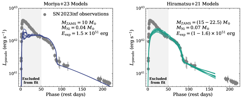
Figure 2: Comparison of our pseudo-bolometric light curve to models from Moriya et al. (2023) (left) and Hiramatsu et al. (2021) (right). While both model grids contain synthetic light curves that reproduce the plateau and nebular phase behaviors of SN 2023ixf, they survey different range of progenitor and explosion properties. The regions shaded in light gray indicate epochs excluded from the $\chi^{2}$ fitting procedure.

3.1 Moriya+23 Accelerated Wind Models

We obtain the large grid of pre-computed multi-frequency hydrodynamic models from Moriya et al. (2023). The grid contains 228,016 synthetic light curves simulated using the multi-group radiation hydrodynamics code STELLA (Blinnikov et al. 1998, 2000, 2006; Blinnikov & Sorokina 2004; Baklanov et al. 2005), based on five RSG progenitor models with initial masses of 10, 12, 14, 16, and 18 $M_{\odot}$ from Sukhbold et al. (2016), evolved with KEPLER (Weaver et al. 1978). Confined CSM density structures following a $\beta$-law wind velocity profile are attached on top the progenitor models, with varying mass-loss rates, CSM extents, and wind acceleration parameters. We refer readers to Moriya et al. (2023) for more details on the setup of the model grid. We retrieve simulated SEDs with a wavelength range from 1 Å to 50,000 Å at different phases with respect to the explosion date. We compute the pseudo-bolometric luminosity by integrating the SEDs from the mean transmission wavelength of $U$ to $z$ bands for each model in the grid. We present a few of the top models in the left panel of Figure 2.

The top models from the Moriya et al. (2023) model grid are consistent with the luminosity of SN 2023ixf on the plateau. They all share the same progenitor and explosion parameters: an initial mass of $M_{\rm ZAMS}=10\ M_{\rm ZAMS}$, a pre-explosion radius of $R=510\ R_{\odot}$, an explosion energy of $E_{\rm exp}=1.5\times 10^{51}$ erg, and a nickel mass of $M_{\rm Ni}=0.04\ M_{\odot}$. The main differences between these models are the CSM parameters. Since we are only concerned with behaviors from the plateau and beyond, we recover a different explosion energy than Moriya & Singh (2024), who performed a similar $\chi^{2}$-minimization search on the model grid, which is expected when simultaneously fitting the initial luminosity excess caused by CSM interaction.

3.2 Hiramatsu+21 CSM-Free Models

While there are models within the Moriya et al. (2023) grid that are consistent with the plateau and nebular phase luminosity, the coarse sampling in $M_{\rm ZAMS}$ raises doubts on whether a low-mass progenitor is the only possibility for SN 2023ixf. Furthermore, the plateau properties are closely related to the progenitor structure, such as the radius and the hydrogen-rich envelope mass (e.g., Popov 1993; Kasen & Woosley 2009; Dessart et al. 2013; Moriya et al. 2016). In this vein, the progenitor models from Sukhbold et al. (2016) may not reflect the true properties of SN 2023ixf. Moreover, the non-uniqueness of light-curve properties as a function of progenitor mass in SNe IIP has been discussed in detail (e.g., Dessart & Hillier 2019; Goldberg et al. 2019; Goldberg & Bildsten 2020), especially when considering variations in stellar structure due to varied stellar mass loss (e.g., Morozova et al. 2015; Dessart et al. 2024).

Motivated by these reasons, we retrieve the CSM-free model grids from Hiramatsu et al. (2021) constructed using Modules for Experiments in Stellar Astrophysics (MESA; Paxton et al. 2011, 2013, 2015, 2018, 2019; Jermyn et al. 2023) + STELLA, and compare them with our observations in the right panel of Figure 2. The advantages of the models from Hiramatsu et al. (2021) are that they survey a wider range of progenitor mass ($10-25\ M_{\odot}$) and they take varied mass-loss efficiencies ($\eta_{\rm wind}=0-3$) into consideration over the lifetime of the RSG progenitors. These extra measures result in a more diverse array of progenitor structures prior to explosion compared to those from Sukhbold et al. (2016). Again, note that we are not attempting to fit the early peak of the light curve, which we assume is dominated by extra luminosity from CSM interaction; we are most interested in matching the late plateau and decay tail from day 50 and onward.

Instead of a low-mass progenitor, we find that the best-fitting models from Hiramatsu et al. (2021) are relatively more massive stars ($M_{\rm ZAMS}>15\ M_{\odot}$) that undergo intense mass-loss (losing $>30\%$ of their initial masses). Such mass loss may be unrealistically high for single RSGs (e.g., Beasor et al. 2020) undergoing standard stellar evolution, and we will discuss the implications of this later in the paper. These progenitor models also have larger radii ($R\approx 680-810\ R_{\odot}$) at the time of explosion, but with lower envelope masses ($\approx 3-5\ M_{\odot}$, compared to $7.2\ M_{\odot}$ for the $M_{\rm ZAMS}=10\ M_{\odot}$ model from Moriya et al. 2023). We derive a ⁵⁶Ni mass of $0.07\ M_{\odot}$ here, which is consistent with the value quoted by Zimmerman et al. (2024), marginally agrees with $0.059\ M_{\odot}$ from Singh et al. (2024), but deviates from $0.04\ M_{\odot}$ inferred using the model grid from Moriya et al. (2023) and $0.05\ M_{\odot}$ from Bersten et al. (2024). Given that relatively low-mass progenitors with little mass loss and higher-mass progenitors with enhanced mass loss can both reproduce plateau behaviors, additional constraints must be imposed to further discern the physical origin of SN 2023ixf.

4 Constraining Progenitor and Light-Curve Models with Pulsation Period

4.1 Degeneracy in Type IIP SN Light Curves

An important caveat of the model grid from Moriya et al. (2023) is the fixed mass-radius relationship of the progenitors when applying explosion models of STELLA. In fact, this caveat applies to any attempt to derive a mass from a grid of progenitor models where each underlying progenitor star exploded is identified with a single progenitor radius at the time of explosion. As shown in Goldberg et al. (2019) and Goldberg & Bildsten (2020), there exist degeneracies (“a family of explosions”) between progenitor radius, ejecta mass, and explosion energy that cannot be lifted with one-to-one mappings of progenitor and explosion properties. These degeneracies can be well-described by the scaling relations of Popov (1993), Kasen & Woosley (2009), Sukhbold et al. (2016), Goldberg et al. (2019), and others. We show the corresponding degeneracy curves for SN 2023ixf using the scaling relations of Goldberg et al. (2019) in Figure 3 (their Eq. 22), calculated with the luminosity at day 50 $L_{50}$, plateau duration $t_{p}$, and ⁵⁶Ni mass $M_{\rm Ni}$, overplotted with the models from Moriya et al. (2023) and Hiramatsu et al. (2021).

Instead of plotting $M_{\rm ej}$, we show the H-rich envelope mass $M_{\rm H,env}$ in Figure 3. The original argument for using $M_{\rm ej}$ to calibrate the scaling relations in Goldberg et al. (2019) was that their models exhibited strong mixing of hydrogen deep into the interior of the star from self-consistent mixing via the Duffell (2016) Rayleigh-Taylor Instability mixing prescription. This resulted in the majority of the ejecta partaking in hydrogen recombination and thus collectively driving the evolution of the SN on the plateau. However, the models in Moriya et al. (2023) (with progenitors from Sukhbold et al. 2016), Hiramatsu et al. (2021), and our own (see the following subsection) contain progenitors that only have zero to moderate amounts of hydrogen mixed into the core. Additionally, in partially-stripped envelopes, the H-rich envelope mass makes up a smaller fraction of the total ejecta mass. Therefore, the envelope mass at the time of explosion is the more appropriate choice to use for comparing to scaling relations here, as it drives the bulk evolution of the luminosity during the photospheric phase.

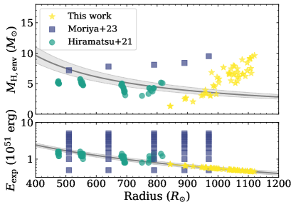
Figure 3: Degeneracy curves for SN 2023ixf recovered from the scaling relations of Goldberg et al. (2019) as a function of progenitor radius. The gray solid lines indicate the H-rich envelope mass (top panel) and explosion energy (bottom panel) required for a given progenitor radius to match the observed SN properties such as plateau duration and luminosity at day 50. For demonstration purposes, the degeneracy curves were constructed with a nickel mass of $M_{\rm Ni}=0.07\ M_{\odot}$. Shaded regions correspond to $1\sigma$ bounds that take the intrinsic scatter of the scaling relations and errors on the parameters used into account. We also show models from Moriya et al. (2023) (navy squares; all possible combination), Hiramatsu et al. (2021) (green circles; top 50 models selected via $\chi^{2}$ fitting), and our own modeling (yellow stars; top 50 models selected via pulsation period).

From Figure 3, it is not surprising to see that the best-fitting models from the pre-computed grid of Moriya et al. (2023) are all consistent with a low-mass progenitor with a higher explosion energy, as the $10\ M_{\odot}$ progenitor model exploded with $E_{\rm exp}=(1.5-2)\times 10^{51}$ erg perfectly intersect both degeneracy curves. The same argument goes for the initially high-mass progenitors from Hiramatsu et al. (2021) that lose significant amounts of mass and end up with larger radii prior to core collapse, thereby only requiring $E_{\rm exp}\approx 10^{51}$ erg (note as well that these models all have similar remaining H envelope mass of $\approx 3-5\ M_{\odot}$, due to the stronger mass-loss prescription adopted in more massive stars). Models that intersect the degeneracy curves are also the best-fitting models selected via $\chi^{2}$ distributions in Section 3, further supporting the choice of using $M_{\rm H,env}$ instead of $M_{\rm ej}$. The ability of these simple scaling laws in predicting explosion properties highlights the crucial need for independent measurements of the progenitor radius in aiding hydrodynamical modeling of SN IIP light curves.

Due to the highly dusty and therefore extincted nature of the progenitor of SN 2023ixf (Jencson et al. 2023; Kilpatrick et al. 2023; Soraisam et al. 2023; Xiang et al. 2024; Van Dyk et al. 2024), however, the measurement of pre-explosion radius is a non-trivial and highly uncertain task. In the next section, we seek to remedy our inability to accurately determine progenitor radius by creating an additional small grid of MESA models with a wide range of progenitor properties, and narrow down viable candidate models via observed variability.

4.2 MESA Progenitor Models Matching Observed Progenitor Variability

An important, unique constraint on the nature of SN 2023ixf’s progenitor comes from the observed IR variability with a perodicity of $P\approx 1100$ days (Soraisam et al., 2023; Jencson et al., 2023; Kilpatrick et al., 2023). RSG variability has been well-studied in galactic and nearby stellar populations (e.g., Jurcevic et al. 2000; Kiss et al. 2006; Percy & Khatu 2014; Soraisam et al. 2018; Conroy et al. 2018; Chatys et al. 2019; Ren et al. 2019), with periods typically ranging from a few hundred to a few thousand days with period-luminosity relations characteristic of fundamental-mode and first-overtone radial pulsations. While the pulsation phase may impact the light curves via the $\approx$10% variation in the progenitor radius at the time of explosion (Goldberg et al., 2020), RSG pulsation periods are very sensitive to the star’s envelope mass, radius, and luminosity (Stothers, 1969; Guo & Li, 2002; Joyce et al., 2020). We thus construct additional models in order to incorporate additional information about the stellar structure provided by the observed progenitor variability.

Using MESA revision 24.03.1, we construct non-rotating, solar-metallicity ($Z=0.02$) models with varying ZAMS masses ($M_{\rm ZAMS}=10–25\ M_{\odot}$ in increments of $0.5\ M_{\odot}$) and convective efficiencies ($\alpha_{\rm MLT}=1.5–3$ in increments of 0.5) in the hydrogen-rich envelope. We note that varying $\alpha_{\rm MLT}$ provides additional variation in the stellar radius (Stothers & Chin, 1995; Massey & Olsen, 2003; Meynet et al., 2015; Goldberg et al., 2022a). We adopt MESA’s “Dutch” prescription for winds with varying efficiency factor ($\eta_{\rm wind}=0–3$ in increments of 0.5), and use modest convective overshooting parameters $f_{\rm ov}=0.01$ and $f_{\rm 0,ov}=0.005$. For reference, a wind efficiency of $\eta_{\rm wind}=1$ under the Dutch scheme translates to a mass-loss rate that is $\sim 10$ higher than measured values for normal RSG winds ($\dot{M}_{\rm wind}\lesssim 10^{-5}\ M_{\odot}\ {\rm yr^{-1}}$; e.g., Beasor et al. 2020). Other inputs are determined following the 12M_pre_ms_to_core_collapse case of the MESA test suite, which is based on the setup described in Section 6 of Paxton et al. (2018) and Farmer et al. (2016).

To compare the candidate RSG progenitor of SN 2023ixf, which exhibited strong variability with a long baseline period of $P\approx 1100$ days (Jencson et al. 2023; Soraisam et al. 2023), we use the the pulsation instrument GYRE (Townsend & Teitler 2013) to identify the period for the fundamental radial ($l=0$) mode at $\approx 7000$ days prior to the onset of core collapse. We plot the period as a function of the hydrogen envelope mass $M_{\rm H,env}$ and progenitor radius at core collapse in Figure 4, which shows that a low envelope mass ($\lesssim 10\ M_{\odot}$) and a large progenitor radius ($\gtrsim 800\ R_{\odot}$) are required to match the observed variability. We note that as in Hiramatsu et al. (2021), we find that many low-mass models ($M_{\rm ZAMS}\lesssim 12.5M_{\odot}$) develop highly degenerate cores and fail during later burning stages that require off-center ignition. While excluding these models may introduce some bias to our sample, most of these low-mass progenitors likely will not have the correct physical properties (e.g., a low envelope mass with a larger radius; see Figure 4) required to satisfy the high fundamental-mode pulsation period observed for SN 2023ixf. We therefore discard these models at this stage.

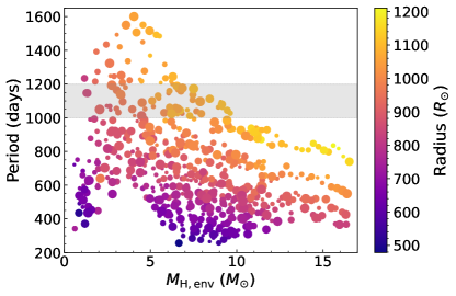
Figure 4: Pulsation period at $\approx$7000 days before core collapse as a function of the hydrogen envelope mass $M_{\rm H,env}$ at explosion. Each model is color-coded by the progenitor radius and the size corresponds to the initial mass $M_{\rm ZAMS}$. The shaded region in gray highlights the models with periods within the range $P=1000-1200$ days, consistent with the observed IR variability in Soraisam et al. (2023) and Jencson et al. (2023).

We continue evolving models with periods in the range of $P=1000-1200$ days through core collapse, then explode the stellar models via a thermal bomb energy deposition by modifying the ccsn_IIp test suite before handing off to the radiation-hydrodynamics software instrument STELLA to create synthetic observables. While exploding progenitor models at the appropriate pulsational phase by injecting a velocity profile proportional to the fundamental mode eigenfunction as done in Goldberg et al. (2020) can provide additional constraints, it is outside the scope of this paper and we leave it as an avenue for improved modeling in the future. As first-order estimates for progenitor and explosion properties, we return to the scaling relations to calculate the explosion energy $E_{\rm exp}$ required to match the plateau properties. Since the scaling relations, as well as $L_{50}$ and $t_{p}$, have intrinsic uncertainties associated with them, we also capture the $1\sigma$ bounds for $E_{\rm exp}$ for a total of three explosion energies for each progenitor model. Due to the large progenitor radii required to reproduce the observed pulsation period, most of our progenitor models favor relatively low-energy explosions in order to simultaneously reproduce the light curve brightness and duration ($E_{\rm exp}<10^{51}\ {\rm erg}$), contrary to previous findings (Hiramatsu et al. 2023; Bersten et al. 2024; Singh et al. 2024). The SN shock propagation is modeled following the prescription of Duffell (2016) for mixing via Rayleigh–Taylor instability until near shock breakout, with the final ⁵⁶Ni scaled to match a total mass of $M_{\rm Ni}=0.07M_{\odot}$ derived in Section 3.2. Here, we do not mix any ⁵⁶Ni into the hydrogen envelope, as it is not clear if and how far ⁵⁶Ni is mixed beyond the core (see, e.g., Kasen & Woosley 2009; Bersten et al. 2011; Dessart et al. 2013; Moriya et al. 2016, for the effects of ⁵⁶Ni mixing on the characteristics of the decay tail).

As baseline measures, we first explore CSM-free explosion models. We use 800 spatial zones for the SN ejecta and 100 frequency bins to yield convergence in the synthetic bolometric and pseudo-bolometric light curves produced by STELLA. Any late-time fallback material produced by reverse shocks from core boundaries interacting with the lowest-velocity inner material is excised via the zero-energy technique described in Paxton et al. (2019) and Goldberg et al. (2019), with an additional standard velocity cut of 500 km s^-1 at the inner boundary at handoff between MESA and STELLA. We find that the low explosion energies inferred for our models are not significantly larger than the magnitude of the binding energy of their progenitors at the time of explosion. As such, we observe non-negligible fallback, with $M_{\rm fallback}\approx 0.5-3.6\ M_{\odot}$. This is also seen in models of some other short-plateau SNe IIP (e.g. Teja et al., 2024). These materials that do not collapse into the initial compact remnant object could supply additional accretion-powered luminosity that interacts with the ejecta and thereby alter the observed light-curve properties (e.g., Dexter & Kasen 2013; Chan et al. 2018; Lisakov et al. 2018; Moriya et al. 2019). We also note that it is only the innermost core layers which experience this fallback, so plateau properties mediated by H-recombination might be unaffected by this fallback until the fall from the plateau, with other signatures of fallback accretion possibly manifesting at much later times. Since the proper treatment of late-time fallback and subsequent accretion onto the proto-neutron star in 1D simulations remains an open question, we therefore caution that our models should be viewed as approximations and may not reflect all physical processes at work.

Table 1: Progenitor and Explosion Properties of our MESA+STELLA Models

	$M_{\rm ZAMS}$	$\eta_{\rm wind}$	$\alpha_{\rm MLT}$	$M_{\rm final}$	$M_{\rm H,env}$	Radius	Period	$E_{\rm exp}$	$M_{\rm ej}$	$M_{\rm fallback}$
Progenitor Model
	($M_{\odot}$)			($M_{\odot}$)	($M_{\odot}$)	($R_{\odot}$)	(days)	($10^{51}$ erg)	($M_{\odot}$)	($M_{\odot}$)
17.5M_eta2.5_alpha2.0	17.5	2.5	2.0	8.74	3.26	994	1138	0.66	6.99	0.78
18.0M_eta1.5_alpha1.5	18.0	1.5	1.5	8.80	3.04	974	1164	0.68	6.98	1.18
20.5M_eta1.5_alpha1.5	20.5	1.5	1.5	9.56	3.03	945	1053	0.48	7.62	1.83
21.5M_eta1.5_alpha1.5	21.5	1.5	1.5	9.90	3.13	950	1031	0.71	7.92	1.64
18.0M_eta2.5_alpha1.5	18.0	2.5	1.5	8.53	3.02	975	1166	0.68	6.85	0.80

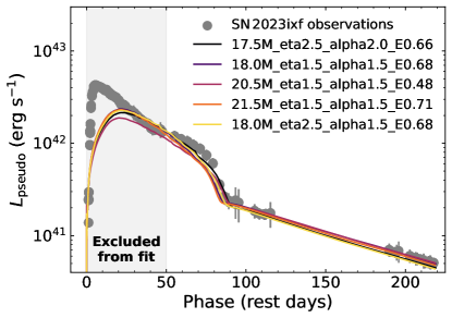
Figure 5: Top five best-fitting CSM-free models for SN 2023ixf. The region shaded in light gray indicates epochs excluded from the $\chi^{2}$ fitting procedure. With the additional constraints from pulsation period and the degeneracy curves, our synthetic light curves recover the plateau properties well. The assumption of $M_{\rm Ni}=0.07\ M_{\odot}$ provides an excellent agreement with observations on the radioactive tail.

We list the progenitor and explosion properties of our top five best-fit models in Table 1 and show the corresponding synthetic light curves in Figure 5. The naming convention follows $\langle M_{\rm ZAMS}\rangle$M_eta$\langle\eta_{\rm wind}\rangle$_alpha$\langle\alpha_{\rm MLT}\rangle$_E$\langle E_{\rm exp}\rangle$. With a more detailed modeling that follows the degenerate scaling relations, we recover high-mass progenitors that shed a significant portion of their hydrogen envelopes to match the plateau behaviors best, similar to our findings in Section 3.2. The models are in excellent agreement with observations, albeit slightly underluminous during later plateau phases ($t\gtrsim 60$ days). The plateau duration and the radioactive tail, however, are in excellent agreement with observations.

In Figure 6 we show the corresponding multi-band light curves for the same models, which are constructed by convolving the SEDs returned by STELLA with the transmission function of each filter ($UBVgriz_{s}$) at each timestep. The luminosity excess in the observed pseudo-bolometric and multi-band light curves compared to our models at $t\gtrsim 60$ days could be explained by the presence of a less dense and extended CSM structure (e.g., Morozova et al. 2017) that supplies more UV radiation. The excess on the radioactive tail in redder bands could be attributed to radiation leaking out from bluer bands, and a more centrally concentrated ⁵⁶Ni distribution could potentially resolve the discrepancies in colors.

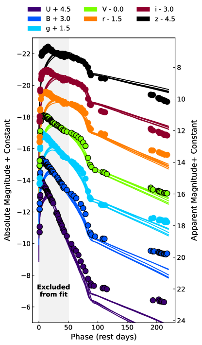
Figure 6: The corresponding multi-band light curves of the models in Figure 5. The region shaded in light gray indicates epochs excluded from the $\chi^{2}$ fitting procedure.

4.3 Steady-State Wind

To account for the missing early-time and plateau luminosity, we explore the addition of steady-state winds on top of each progenitor model. As found in Hiramatsu et al. (2023), to match the peak luminosity with a steady-state wind with a velocity of $v_{\rm wind}=115$ km s^-1 (Smith et al. 2023) requires $\dot{M}_{\rm wind}\geq 0.3\ M_{\odot}\ {\rm yr^{-1}}$ over a duration of $t_{\rm wind}=1-2\ {\rm yr}$ prior to explosion. Also noted in Morozova et al. (2017) is that for any given mass-loss rate, the radial extent of the CSM itself heavily influences the peak luminosity and decline rate post-maximum luminosity. Therefore, we attach CSM structures following a steady-state wind with $\dot{M}_{\rm wind}=10^{-2}-1\ M_{\odot}\ {\rm yr^{-1}}$ (0.5 dex increments) and extents of $R_{\rm wind}=2-10\times 10^{14}\ {\rm cm}$ ($2\times 10^{14}$ increments, which correspond to a mass-loss duration of $t_{\rm wind}\approx 0.5-2.8$ yrs prior to explosion) on top of the five best-fitting CSM-free progenitor models. We use an additional 200 spatial zones for the CSM attached in STELLA, on top of the 800 zones used for the SN ejecta. We show the effects of varying the CSM extent and mass-loss rate for 17.5M_eta2.5_alpha2.5_E0.66 in Figure 7.

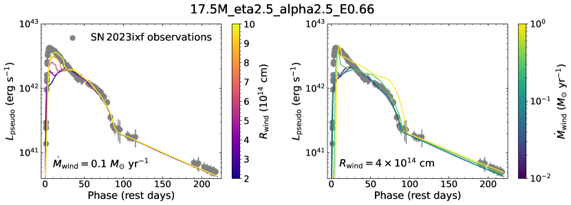
Figure 7: Comparison of the pseudo-bolometric light curve of SN 2023ixf with CSM from a steady-state wind with a velocity of 115 km s^-1 on top of 17.5M_eta2.5_alpha2.5_E0.66. We show the effects of varying the extent for a fixed mass-loss rate ($R_{\rm wind}$; left) and varying the mass-loss rate for a fixed extent ($\dot{M}_{\rm wind}$; right).

Akin to previous studies of CSM interaction in SN light curves, the primary effect of varying the CSM extent is raising the peak luminosity, while varying the mass-loss rate raises the brightness and prolong the plateau duration. While some combinations of $\dot{M}_{\rm wind}$ and $R_{\rm wind}$ can reasonably reproduce the luminosity during first $\approx 20$ days of the SN evolution, the rise times are too long and the decline rates are inconsistent compared to observations. Nevertheless, a steady-state wind is likely not an accurate depiction of the CSM configuration for SN 2023ixf, as the measured wind velocity of 115 km s^-1 is much higher than a typical RSG wind velocity of $\sim 20$ km s^-1 and likely requires radiative acceleration (Moriya et al. 2018; Tsuna et al. 2023). We discuss alternative CSM configurations in Section 5. Similar to the plateau luminosity, there likely also exists a degeneracy between progenitor, explosion, and CSM properties that require careful treatments via independent constraints from other avenues, such as simultaneously modeling the evolution of Fe II line velocities and the time of disappearance of narrow line features (Martinez et al. 2024).

5 Discussion

5.1 Differences Compared to Previous Work

Since SN 2023ixf’s discovery, numerous studies have been published in an effort to unveil its properties, ranging from pre-explosion observations of the SN site to properties of the SN itself. There is, however, a disagreement on the initial mass inferred from pre-explosion observations, with a wide range of values of $M_{\rm ZAMS}=8-20\ M_{\odot}$. Previous hydrodynamical modeling (e.g., Bersten et al. 2024; Hiramatsu et al. 2023; Moriya & Singh 2024; Singh et al. 2024) pointed to low H envelope masses, and thus seemed to agree with the lower end of initial mass estimation from some progenitor studies (Kilpatrick et al. 2023; Neustadt et al. 2024; Van Dyk et al. 2024; Xiang et al. 2024).

From our detailed light-curve modeling, however, we have found that, contrary to previous studies (e.g., Hiramatsu et al. 2023; Bersten et al. 2024; Moriya & Singh 2024; Singh et al. 2024), SN 2023ixf does not need to be an energetic explosion of a low-mass progenitor. Instead, a more massive RSG progenitor ($M_{\rm ZAMS}=17-22\ M_{\odot}$) that lost more than half of its ZAMS mass can also reproduce observed light-curve behaviors. This work is the first light-curve modeling effort that derives a progenitor mass that is consistent with higher initial masses (Jencson et al. 2023; Niu et al. 2023; Qin et al. 2023; Soraisam et al. 2023), and is further supported by the independent constraint of the progenitor star’s pulsation period.

Both these options—a lower initial mass with less mass loss, as compared to a higher initial mass with more mass loss—can end up at the time of explosion with the right combination of H-envelope mass and stellar radius (see the top panel of Figure 3). This is the main reason that any family of models can adequately approximate the light-curve shape when exploded with the correct explosion energy. It is important to recognize that these model differences are completely artificial because they simply depend on the adopted mass-loss prescription, none of which resemble the much lower mass-loss rates of actual RSG winds (e.g., Beasor et al. 2020, 2023; Antoniadis et al. 2024; Decin et al. 2024). With more realistic mass-loss rates, single RSGs at all initial masses lose very little mass via steady winds during the RSG phase, so single RSGs should retain most of their H envelopes until the time of explosion (Beasor et al., 2021). Additionally, as noted by Beasor et al. (2020), the baseline “Dutch” mass-loss prescription overestimates normal RSG winds by a factor of $\sim$10, whereas the winds with $\eta_{\rm wind}$ values of 1.5-2.5 are even more artificially inflated. Nevertheless, the models with extremely strong winds seem to do a good job of yielding a final envelope mass that explains the light-curve shape of SN 2023ixf.

5.2 A Binary Companion Stripping the Envelope?

In the context of RSG evolution, the most plausible way to interpret the agreement of observations with our models that have artificially inflated mass-loss rates is not that the progenitor had a bizarrely strong wind (even though this is how the models are engineered to lose their envelopes). Rather, a much more likely scenario is that the progenitor was in a binary system, and the removal of much of the H envelope was accomplished via stripping by close encounters with its companion star. If the progenitor did in fact have a higher initial mass, as our analysis of the progenitor’s pulsation period seems to require, then strong mass stripping via mass transfer to a binary companion is essential to achieve the low envelope mass required to explain SN 2023ixf. This is consistent with the growing observational consensus that most massive stars live in binaries (e.g., Sana et al. 2012; de Mink et al. 2013; Moe & Di Stefano 2017) and the lack of bright precursor outbursts before SN 2023ixf (Dong et al. 2023; Hiramatsu et al. 2023; Neustadt et al. 2024; Ransome et al. 2024). Although, some studies show that binary interaction may be the formation channel for only a modest fraction of all SNe IIP (e.g., Sravan et al. 2019; Ercolino et al. 2024), which could make SN 2023ixf an unusual case.

While binary interaction is a natural explanation for the low envelope mass inferred in this work, there are several caveats. Our study requires that a large mass of order 10 $M_{\odot}$ was removed by the star by some mechanism prior in its evolution in order to attain the appropriate properties for the observed pulsation period (see Figure 4). This might correspond to either Case A or Case B mass transfer, where Roche lobe overflow (RLOF) occurs during core H burning and before core He depletion, respectively (see Marchant & Bodensteiner 2023 for a review). Multiple studies predict, however, that the donor stars in these scenarios inevitably end up as either yellow supergiants or blue supergiants, if not completely stripped to become Wolf-Rayet stars (e.g., Götberg et al. 2017; Laplace et al. 2020; Sen et al. 2022; Marchant & Bodensteiner 2023). This would seem at odds with the identification of SN 2023ixf’s progenitor as a RSG from pre-explosion imaging (e.g., Jencson et al. 2023; Soraisam et al. 2023; Van Dyk et al. 2024), unless the progenitor swelled up to become red in its final years.

Perhaps a more suitable scenario for SN 2023ixf is a binary system that has undergone Case C (RLOF after core He depletion) or Case BC mass transfer (Case B followed by Case C), which is consistent with simulations of interacting wide massive binaries (Ercolino et al. 2024). We caution, however, that the presence of a nearby companion close to explosion (i.e., the explosion took place during binary interaction or soon after) may modify the geometry of the progenitor, which may violate the spherical symmetry assumed when calculating the pulsation period using GYRE. A more detailed analysis of the pulsation period for a non-spherical star may then be necessary to further constrain the progenitor mass. Nevertheless, even without the aid of pulsation period, models with high initial mass and strong envelope mass loss are still contenders for the progenitor of SN 2023ixf, as indicated by our light-curve comparison in Section 3.2. Case BC mass transfer also paints a more self-consistent picture for the dense CSM in the vicinity of the progenitor, where most of the envelope mass is stripped during core He burning and the CSM is formed during later interactions. This is supported by Matsuoka & Sawada (2024), where the mass-loss rates achieved via binary interactions during the final evolutionary stages of RSG stars are comparable to values inferred for SN 2023ixf.

Spectropolarimetric data from Vasylyev et al. (2023) and Singh et al. (2024) also revealed a continuum polarization level of $\approx 1\%$ one day after discovery, before dropping to $\approx 0.5\%$ and eventually disappearing along with narrow emission-line features over the first $\sim 5$ days of SN 2023ixf’s evolution. This indicates that either the pre-explosion mass-loss was highly asymmetric in nature (which is in agreement with the results of high-resolution spectroscopy in the first week after explosion; Smith et al. 2023), the shock broke out aspherically (Matzner et al. 2013; Goldberg et al. 2022b; Singh et al. 2024), or both. A disk-like CSM geometry is different from the spherically symmetric mass loss assumed in most models for SN 2023ixf in the literature. It does, however, seem in obvious agreement with the hypothesis that the progenitor was in an interacting binary system, as noted above. The motion of a nearby companion star, or perhaps a companion embedded in the common envelope of the inflated RSG progenitor, could drive mass ejection concentrated toward the equatorial plane leading up to the time of explosion (e.g., Smith & Arnett 2014; Pejcha et al. 2016). In this framework, a CSM structure that consists of a dense, asymmetric disk or torus in conjunction with a low-density, extended wind (Smith et al. 2023; Singh et al. 2024) may be the most plausible configuration for SN 2023ixf.

5.3 Other Possible Mechanisms for Envelope Stripping and CSM Formation

Can some other mass-loss mechanism besides binary mass stripping account for the loss of most of SN 2023ixf’s H envelope? Currently, there is no observational evidence for any bright outbursts in SN 2023ixf’s progenitor star for the last $\sim 15$ years (Dong et al. 2023; Hiramatsu et al. 2023; Neustadt et al. 2024; Ransome et al. 2024). More importantly, in the case of SN 2023ixf, brief signatures of shock interaction limit the CSM to a total mass of $\lesssim 0.1\ M_{\odot}$ (Bostroem et al. 2023; Jacobson-Galán et al. 2023), lost in the few years just before core collapse, with a much weaker preceding stellar wind (Bostroem et al. 2024). The dense CSM has nowhere near enough mass to account for the $\sim 10M_{\odot}$ lost during the star’s life, so the removal of the H envelope must have occurred much earlier in the progenitor’s evolution. Thus, any eruptive mass-loss mechanism tied to instabilities in the final nuclear burning phases (Ne, O, and Si burning; Arnett & Meakin 2011; Smith & Arnett 2014; Woosley & Heger 2015) or gravity waves excited during those same phases (Quataert & Shiode 2012; Shiode et al. 2013; Shiode & Quataert 2014; Fuller 2017; Wu & Fuller 2021, 2022) cannot be the culprit for shedding most of the H envelope.

There have been some suggestions for how to achieve strong RSG mass loss in the literature. Cheng et al. (2024) postulated that local super-Eddington luminosities due to the presence of opacity peaks in the stellar envelope during the transition from the main sequence to the red giant branch can lead to short-timescale, likely eruptive, mass-loss events of up to $\approx 10^{-3}\ M_{\odot}\ {\rm yr^{-1}}$ for stars with $M_{\rm ZAMS}\lesssim 20\ M_{\odot}$. However, this means that the progenitor would need to spend the entire $\sim 10^{4}$ years across the Hertzsprung gap in eruption in order to achieve the $\sim 10\ M_{\odot}$ loss in its envelope, which is unlikely, and generally not seen in their models below $30\ M_{\odot}$. Aside from eruptive mass loss, there have been other strong mass-loss mechanisms proposed for RSGs. For example, radial pulsations driven by a $\kappa$-mechanism in the partially ionized hydrogen envelope may produce sufficiently large pulsation amplitudes to create a “superwind” (e.g., Heger et al. 1997; Yoon & Cantiello 2010). The idea of RSG “boil-off” proposed by Fuller & Tsuna (2024), based on the large-scale turbulent motion of dense plumes of convective material near the photosphere of RSGs (Chiavassa et al. 2011, 2024; Goldberg et al. 2022a), is another mechanism that, hypothetically, could drive enhanced mass-loss episodes of up to $\sim 10^{-5}\ M_{\odot}\ {\rm yr^{-1}}$ for stars with $M_{\rm ZAMS}\lesssim 20\ M_{\odot}$.

In order to strip such a significant portion of the progenitor’s envelope, however, would require either the pulsation-driven superwinds or turbulent mass ejections to have been sustained for a long duration, as required by the low envelope mass and the pulsation period. This may be in conflict with observations of normal RSGs, which limit any enhanced mass-loss phases to about 1% of the time during the post-main-sequence phase or less (Beasor & Smith, 2022). With a much lower mass inferred for the CSM, any such strong mass loss that removed $\sim 10\ M_{\odot}$ from the envelope must have occurred at a much earlier evolutionary stage (probably before core C burning), and weakened (if not completely turned off) long before core collapse. The reason that this is problematic is because these strong wind mechanisms tend to scale with close proximity to the luminosity-to-mass ratio of the progenitor, which monotonically increases as the star evolves up the RSG branch and as it continually loses more mass. One therefore does not expect these mechanisms to slow down or shut off with a significant H envelope remaining; instead, they should ramp up or at least stay constant when the remaining stellar lifetime is shorter than the thermal timescale across the entire envelope.

As noted above, the large mass of $\sim 10\ M_{\odot}$ that was evidently removed from the H envelope was nowhere near the star at the time of death. Combined with the low remaining H-envelope mass ($\lesssim 3\ M_{\odot}$) of our models, current evidence seems to imply that whatever caused the envelope mass loss may not be the same mechanism as that which formed the CSM, nor can it be a continuous process. If such extreme wind mass loss was responsible for stripping the envelope, it is unclear when and what could trigger such an abrupt halt to these mechanisms. Furthermore, the mass-loss rates inferred by these processes are hard to reconcile with observations of nearby RSG populations, which do not show evidence of such strong wind mass loss during their normal He burning evolution (Beasor et al. 2020, 2023; Antoniadis et al. 2024; Decin et al. 2024), and therefore unlikely to strip such a large portion of the H envelope. On the other hand, the dense CSM has more direct observational constraints, and is less in conflict with observations of normal RSGs, since it must have been formed in a very brief phase. Thus, whatever mechanism gave rise to SN 2023ixf’s strong but very brief CSM interaction was therefore likely a different mass-loss or mass-loading episode than what removed most of the H envelope.

Are there other mechanisms that could produce the dense CSM in the vicinity of SN 2023ixf’s progenitor? While bright outbursts have not been detected, observations do not yet rule out the possibility that the progenitor had faint outbursts on shorter timescales compared to the cadence of these dedicated precursor searches (Davies et al. 2022; Dong et al. 2023). Such faint and brief outbursts may contribute to the CSM around the progenitor at the time of explosion. Pulsation-driven superwinds and RSG boil-offs, while not likely to be the cause for the strong envelope stripping, may still be good candidates for forming the immediate CSM structures around SN 2023ixf’s progenitor. When taken together, the combination of pulsation-driven superwinds and convectively-levitated envelope materials have also been proposed as a way to create a long-lived “effervescent zone” around the progenitor star (Soker 2021, 2023). Although, a stagnant effervescent zone may be in tension with the high outflow velocity in the CSM of SN 2023ixf (Smith et al. 2023). We additionally emphasize that the strengths of these phenomena (eruptions/pulsation-driven superwinds/RSG boil-offs/effervescent zones) are amplified with increasing progenitor luminosity, which would be more consistent with our claim of a relatively high initial mass based on the progenitor’s long pulsation period, as compared to an initially lower mass star suggested in other studies.

With current observational constraints, we cannot confidently rule out the idea that enhanced wind mass loss contributes in some way at an earlier phase of the progenitor’s evolution. Follow-up observations in the next decade will be crucial for determining whether any additional dense shells of CSM also exist far away from the progenitor of SN 2023ixf, as in the case of several SNe IIP that showed signatures of late-time CSM interaction years after explosion (e.g., Maguire et al. 2010; Prieto et al. 2012; Mauerhan et al. 2017; Andrews & Smith 2018; Weil et al. 2020). Regardless, binary mass stripping still remains the most straightforward and self-consistent explanation for removing most of SN 2023ixf’s envelope and shaping the immediate dense CSM, even with the aforementioned caveats in Section 5.2, and follow-up observations could similarly reveal any surviving companion. Nevertheless, these are only a few alternatives to produce strong mass loss responsible for the envelope mass loss and the formation of CSM around RSGs. Together, they highlight the diversity of physical processes and formation channels that could produce the progenitor and CSM structures of SNe IIP.

6 Conclusions

We present extensive follow-up photometric observations of SN 2023ixf in the first year of its evolution. By comparing the pseudo-bolometric light curve to available grids of hydrodynamical models, we find that the plateau properties can be recovered with drastically varying physical parameters for the SN and its progenitor, owing to previously established degeneracies between explosion and progenitor properties. Motivated by this, we construct additional numerical progenitor and light-curve models. For the first time, we impose an additional constraint drawn from the observed period of the progenitor star’s pre-explosion variability.

Our results suggest that SN 2023ixf may have originated from the explosion of an initially massive ($M_{\rm ZAMS}\gtrsim 17\ M_{\odot}$) RSG progenitor star, with an explosion energy of $\approx 7\times 10^{50}$ erg, and a ⁵⁶Ni production of 0.07 $M_{\odot}$. Single-star models that agree with the observed variability of $\approx 1100$ days are characterized by a lower than usual envelope mass ($\lesssim 3\ M_{\odot}$) and a pre-explosion radius $\gtrsim 950\ R_{\odot}$. We hypothesize that the RSG progenitor likely experienced a sustained period of intense mass-loss that removed the majority of its H-rich envelope, probably due to mass stripping by a binary companion.

Future UV observations of the SN site could help detect or constrain the presence of a surviving companion star and delineate a more complete picture of the physical origin of SN 2023ixf. With the commencement of the Vera C. Rubin Observatory Legacy Survey of Space and Time (LSST; Ivezić et al. 2019) in 2025, high-cadence monitoring of nearby RSG populations may become increasingly common. The methodology presented in this work that utilizes RSG variability as an independent constraint may offer an alternative way to break scaling degeneracies in future SN IIP light-curve modeling.

References

- Albareti et al. (2017) Albareti, F. D., Allende Prieto, C., Almeida, A., et al. 2017, ApJS, 233, 25
- Anderson et al. (2014) Anderson, J. P., González-Gaitán, S., Hamuy, M., et al. 2014, ApJ, 786, 67
- Andrews & Smith (2018) Andrews, J. E., & Smith, N. 2018, MNRAS, 477, 74
- Andrews et al. (2019) Andrews, J. E., Sand, D. J., Valenti, S., et al. 2019, ApJ, 885, 43
- Andrews et al. (2024) Andrews, J. E., Pearson, J., Hosseinzadeh, G., et al. 2024, ApJ, 965, 85
- Antoniadis et al. (2024) Antoniadis, K., Bonanos, A. Z., de Wit, S., et al. 2024, A&A, 686, A88
- Arnett & Meakin (2011) Arnett, W. D., & Meakin, C. 2011, ApJ, 741, 33
- Astropy Collaboration et al. (2018) Astropy Collaboration, Price-Whelan, A. M., Sipőcz, B. M., et al. 2018, AJ, 156, 123
- Baklanov et al. (2005) Baklanov, P. V., Blinnikov, S. I., & Pavlyuk, N. N. 2005, Astronomy Letters, 31, 429
- Beasor & Davies (2018) Beasor, E. R., & Davies, B. 2018, MNRAS, 475, 55
- Beasor et al. (2021) Beasor, E. R., Davies, B., & Smith, N. 2021, ApJ, 922, 55
- Beasor et al. (2020) Beasor, E. R., Davies, B., Smith, N., et al. 2020, MNRAS, 492, 5994
- Beasor et al. (2023) Beasor, E. R., Davies, B., Smith, N., et al. 2023, MNRAS, 524, 2460
- Beasor & Smith (2022) Beasor, E. R., & Smith, N. 2022, ApJ, 933, 41
- Berger et al. (2023) Berger, E., Keating, G. K., Margutti, R., et al. 2023, ApJ, 951, L31
- Bersten et al. (2011) Bersten, M. C., Benvenuto, O., & Hamuy, M. 2011, ApJ, 729, 61
- Bersten et al. (2024) Bersten, M. C., Orellana, M., Folatelli, G., et al. 2024, A&A, 681, L18
- Blinnikov et al. (2000) Blinnikov, S., Lundqvist, P., Bartunov, O., Nomoto, K., & Iwamoto, K. 2000, ApJ, 532, 1132
- Blinnikov & Sorokina (2004) Blinnikov, S., & Sorokina, E. 2004, Ap&SS, 290, 13
- Blinnikov et al. (1998) Blinnikov, S. I., Eastman, R., Bartunov, O. S., Popolitov, V. A., & Woosley, S. E. 1998, ApJ, 496, 454
- Blinnikov et al. (2006) Blinnikov, S. I., Röpke, F. K., Sorokina, E. I., et al. 2006, A&A, 453, 229
- Boian & Groh (2019) Boian, I., & Groh, J. H. 2019, A&A, 621, A109
- Bostroem et al. (2023) Bostroem, K. A., Pearson, J., Shrestha, M., et al. 2023, ApJ, 956, L5
- Bostroem et al. (2024) Bostroem, K. A., Sand, D. J., Dessart, L., et al. 2024, arXiv e-prints, arXiv:2408.03993
- Brown et al. (2013) Brown, T. M., Baliber, N., Bianco, F. B., et al. 2013, PASP, 125, 1031
- Bruch et al. (2021) Bruch, R. J., Gal-Yam, A., Schulze, S., et al. 2021, ApJ, 912, 46
- Bruch et al. (2023) Bruch, R. J., Gal-Yam, A., Yaron, O., et al. 2023, ApJ, 952, 119
- Bullivant et al. (2018) Bullivant, C., Smith, N., Williams, G. G., et al. 2018, MNRAS, 476, 1497
- Chan et al. (2018) Chan, C., Müller, B., Heger, A., Pakmor, R., & Springel, V. 2018, ApJ, 852, L19
- Chandra et al. (2024) Chandra, P., Chevalier, R. A., Maeda, K., Ray, A. K., & Nayana, A. J. 2024, ApJ, 963, L4
- Chatys et al. (2019) Chatys, F. W., Bedding, T. R., Murphy, S. J., et al. 2019, MNRAS, 487, 4832
- Cheng et al. (2024) Cheng, S. J., Goldberg, J. A., Cantiello, M., et al. 2024, arXiv e-prints, arXiv:2405.12274
- Chiavassa et al. (2011) Chiavassa, A., Freytag, B., Masseron, T., & Plez, B. 2011, A&A, 535, A22
- Chiavassa et al. (2024) Chiavassa, A., Kravchenko, K., & Goldberg, J. A. 2024, Living Reviews in Computational Astrophysics, 10, 2
- Conroy et al. (2018) Conroy, C., Strader, J., van Dokkum, P., et al. 2018, ApJ, 864, 111
- Davies & Beasor (2018) Davies, B., & Beasor, E. R. 2018, MNRAS, 474, 2116
- Davies & Beasor (2020) Davies, B., & Beasor, E. R. 2020, MNRAS, 493, 468
- Davies et al. (2022) Davies, B., Plez, B., & Petrault, M. 2022, MNRAS, 517, 1483
- de Mink et al. (2013) de Mink, S. E., Langer, N., Izzard, R. G., Sana, H., & de Koter, A. 2013, ApJ, 764, 166
- Decin et al. (2024) Decin, L., Richards, A. M. S., Marchant, P., & Sana, H. 2024, A&A, 681, A17
- Dessart et al. (2024) Dessart, L., Gutiérrez, C. P., Ercolino, A., Jin, H., & Langer, N. 2024, A&A, 685, A169
- Dessart & Hillier (2005) Dessart, L., & Hillier, D. J. 2005, A&A, 437, 667
- Dessart & Hillier (2019) Dessart, L., & Hillier, D. J. 2019, A&A, 625, A9
- Dessart et al. (2013) Dessart, L., Hillier, D. J., Waldman, R., & Livne, E. 2013, MNRAS, 433, 1745
- Dexter & Kasen (2013) Dexter, J., & Kasen, D. 2013, ApJ, 772, 30
- Dong et al. (2021) Dong, Y., Valenti, S., Bostroem, K. A., et al. 2021, ApJ, 906, 56
- Dong et al. (2023) Dong, Y., Sand, D. J., Valenti, S., et al. 2023, ApJ, 957, 28
- Duffell (2016) Duffell, P. C. 2016, ApJ, 821, 76
- Ercolino et al. (2024) Ercolino, A., Jin, H., Langer, N., & Dessart, L. 2024, A&A, 685, A58
- Farmer et al. (2016) Farmer, R., Fields, C. E., Petermann, I., et al. 2016, ApJS, 227, 22
- Ferrari et al. (2024) Ferrari, L., Folatelli, G., Ertini, K., Kuncarayakti, H., & Andrews, J. 2024, arXiv e-prints, arXiv:2406.00130
- Fitzpatrick (1999) Fitzpatrick, E. L. 1999, PASP, 111, 63
- Foreman-Mackey et al. (2013) Foreman-Mackey, D., Hogg, D. W., Lang, D., & Goodman, J. 2013, PASP, 125, 306
- Förster et al. (2018) Förster, F., Moriya, T. J., Maureira, J. C., et al. 2018, Nature Astronomy, 2, 808
- Fuller (2017) Fuller, J. 2017, MNRAS, 470, 1642
- Fuller & Tsuna (2024) Fuller, J., & Tsuna, D. 2024, The Open Journal of Astrophysics, 7, 47
- Gal-Yam et al. (2014) Gal-Yam, A., Arcavi, I., Ofek, E. O., et al. 2014, Nature, 509, 471
- Garnavich & Ann (1994) Garnavich, P. M., & Ann, H. B. 1994, AJ, 108, 1002
- Goldberg & Bildsten (2020) Goldberg, J. A., & Bildsten, L. 2020, ApJ, 895, L45
- Goldberg et al. (2019) Goldberg, J. A., Bildsten, L., & Paxton, B. 2019, ApJ, 879, 3
- Goldberg et al. (2020) Goldberg, J. A., Bildsten, L., & Paxton, B. 2020, ApJ, 891, 15
- Goldberg et al. (2022a) Goldberg, J. A., Jiang, Y.-F., & Bildsten, L. 2022a, ApJ, 929, 156
- Goldberg et al. (2022b) Goldberg, J. A., Jiang, Y.-F., & Bildsten, L. 2022b, ApJ, 933, 164
- Götberg et al. (2017) Götberg, Y., de Mink, S. E., & Groh, J. H. 2017, A&A, 608, A11
- Grefenstette et al. (2023) Grefenstette, B. W., Brightman, M., Earnshaw, H. P., Harrison, F. A., & Margutti, R. 2023, ApJ, 952, L3
- Groh (2014) Groh, J. H. 2014, A&A, 572, L11
- Guo & Li (2002) Guo, J. H., & Li, Y. 2002, ApJ, 565, 559
- Heger et al. (1997) Heger, A., Jeannin, L., Langer, N., & Baraffe, I. 1997, A&A, 327, 224
- Henden et al. (2016) Henden, A. A., Templeton, M., Terrell, D., et al. 2016, VizieR Online Data Catalog: AAVSO Photometric All Sky Survey (APASS) DR9 (Henden+, 2016), VizieR On-line Data Catalog: II/336. Originally published in: 2015AAS…22533616H
- Hillier & Dessart (2019) Hillier, D. J., & Dessart, L. 2019, A&A, 631, A8
- Hiramatsu et al. (2021) Hiramatsu, D., Howell, D. A., Moriya, T. J., et al. 2021, ApJ, 913, 55
- Hiramatsu et al. (2023) Hiramatsu, D., Tsuna, D., Berger, E., et al. 2023, ApJ, 955, L8
- Hosseinzadeh et al. (2023a) Hosseinzadeh, G., Bostroem, K. A., & Gomez, S. 2023a, Light Curve Fitting, v0.8.0, Zenodo, doi:10.5281/zenodo.7872772
- Hosseinzadeh et al. (2018) Hosseinzadeh, G., Valenti, S., McCully, C., et al. 2018, ApJ, 861, 63
- Hosseinzadeh et al. (2022) Hosseinzadeh, G., Kilpatrick, C. D., Dong, Y., et al. 2022, ApJ, 935, 31
- Hosseinzadeh et al. (2023b) Hosseinzadeh, G., Farah, J., Shrestha, M., et al. 2023b, ApJ, 953, L16
- Howell & Global Supernova Project (2017) Howell, D. A., & Global Supernova Project. 2017, in American Astronomical Society Meeting Abstracts, Vol. 230, American Astronomical Society Meeting Abstracts #230, 318.03
- Hunter (2007) Hunter, J. D. 2007, CSE, 9, 90
- Itagaki (2023) Itagaki, K. 2023, Transient Name Server Discovery Report, 2023-1158, 1
- Ivezić et al. (2019) Ivezić, Ž., Kahn, S. M., Tyson, J. A., et al. 2019, ApJ, 873, 111
- Jacobson-Galán et al. (2023) Jacobson-Galán, W. V., Dessart, L., Margutti, R., et al. 2023, ApJ, 954, L42
- Jacobson-Galán et al. (2024) Jacobson-Galán, W. V., Dessart, L., Davis, K. W., et al. 2024, arXiv e-prints, arXiv:2403.02382
- Jencson et al. (2023) Jencson, J. E., Pearson, J., Beasor, E. R., et al. 2023, ApJ, 952, L30
- Jermyn et al. (2023) Jermyn, A. S., Bauer, E. B., Schwab, J., et al. 2023, ApJS, 265, 15
- Joyce et al. (2020) Joyce, M., Leung, S.-C., Molnár, L., et al. 2020, ApJ, 902, 63
- Jurcevic et al. (2000) Jurcevic, J. S., Pierce, M. J., & Jacoby, G. H. 2000, MNRAS, 313, 868
- Kasen & Woosley (2009) Kasen, D., & Woosley, S. E. 2009, ApJ, 703, 2205
- Khazov et al. (2016) Khazov, D., Yaron, O., Gal-Yam, A., et al. 2016, ApJ, 818, 3
- Kilpatrick et al. (2023) Kilpatrick, C. D., Foley, R. J., Jacobson-Galán, W. V., et al. 2023, ApJ, 952, L23
- Kiss et al. (2006) Kiss, L. L., Szabó, G. M., & Bedding, T. R. 2006, MNRAS, 372, 1721
- Landolt (1983) Landolt, A. U. 1983, AJ, 88, 439
- Landolt (1992) Landolt, A. U. 1992, AJ, 104, 340
- Laplace et al. (2020) Laplace, E., Götberg, Y., de Mink, S. E., Justham, S., & Farmer, R. 2020, A&A, 637, A6
- Leavitt (1908) Leavitt, H. S. 1908, Annals of Harvard College Observatory, 60, 87
- Li et al. (2024) Li, G., Hu, M., Li, W., et al. 2024, Nature, 627, 754
- Li et al. (2006) Li, W., Van Dyk, S. D., Filippenko, A. V., et al. 2006, ApJ, 641, 1060
- Lisakov et al. (2018) Lisakov, S. M., Dessart, L., Hillier, D. J., Waldman, R., & Livne, E. 2018, MNRAS, 473, 3863
- Lundquist et al. (2023) Lundquist, M., O’Meara, J., & Walawender, J. 2023, Transient Name Server AstroNote, 160, 1
- Maguire et al. (2010) Maguire, K., Di Carlo, E., Smartt, S. J., et al. 2010, MNRAS, 404, 981
- Marchant & Bodensteiner (2023) Marchant, P., & Bodensteiner, J. 2023, arXiv e-prints, arXiv:2311.01865
- Martinez et al. (2024) Martinez, L., Bersten, M. C., Folatelli, G., Orellana, M., & Ertini, K. 2024, A&A, 683, A154
- Martinez et al. (2022a) Martinez, L., Bersten, M. C., Anderson, J. P., et al. 2022a, A&A, 660, A40
- Martinez et al. (2022b) Martinez, L., Bersten, M. C., Anderson, J. P., et al. 2022b, A&A, 660, A41
- Massey & Olsen (2003) Massey, P., & Olsen, K. A. G. 2003, AJ, 126, 2867
- Matsuoka & Sawada (2024) Matsuoka, T., & Sawada, R. 2024, ApJ, 963, 105
- Matthews et al. (2023) Matthews, D., Margutti, R., AJ, N., et al. 2023, Transient Name Server AstroNote, 180, 1
- Matzner et al. (2013) Matzner, C. D., Levin, Y., & Ro, S. 2013, ApJ, 779, 60
- Mauerhan et al. (2017) Mauerhan, J. C., Van Dyk, S. D., Johansson, J., et al. 2017, ApJ, 834, 118
- Mauron & Josselin (2011) Mauron, N., & Josselin, E. 2011, A&A, 526, A156
- Meynet et al. (2015) Meynet, G., Chomienne, V., Ekström, S., et al. 2015, A&A, 575, A60
- Moe & Di Stefano (2017) Moe, M., & Di Stefano, R. 2017, ApJS, 230, 15
- Moriya et al. (2018) Moriya, T. J., Förster, F., Yoon, S.-C., Gräfener, G., & Blinnikov, S. I. 2018, MNRAS, 476, 2840
- Moriya et al. (2019) Moriya, T. J., Müller, B., Chan, C., Heger, A., & Blinnikov, S. I. 2019, ApJ, 880, 21
- Moriya et al. (2016) Moriya, T. J., Pruzhinskaya, M. V., Ergon, M., & Blinnikov, S. I. 2016, MNRAS, 455, 423
- Moriya & Singh (2024) Moriya, T. J., & Singh, A. 2024, arXiv e-prints, arXiv:2406.00928
- Moriya et al. (2023) Moriya, T. J., Subrayan, B. M., Milisavljevic, D., & Blinnikov, S. I. 2023, PASJ, 75, 634
- Morozova et al. (2015) Morozova, V., Piro, A. L., Renzo, M., et al. 2015, ApJ, 814, 63
- Morozova et al. (2017) Morozova, V., Piro, A. L., & Valenti, S. 2017, ApJ, 838, 28
- Morozova et al. (2018) Morozova, V., Piro, A. L., & Valenti, S. 2018, ApJ, 858, 15
- Nadyozhin (1994) Nadyozhin, D. K. 1994, ApJS, 92, 527
- Neustadt et al. (2024) Neustadt, J. M. M., Kochanek, C. S., & Smith, M. R. 2024, MNRAS, 527, 5366
- Niemela et al. (1985) Niemela, V. S., Ruiz, M. T., & Phillips, M. M. 1985, ApJ, 289, 52
- Niu et al. (2023) Niu, Z., Sun, N.-C., Maund, J. R., et al. 2023, ApJ, 955, L15
- Oliphant (2006) Oliphant, T. E. 2006, A guide to NumPy (USA: Trelgol Publishing)
- Panjkov et al. (2023) Panjkov, S., Auchettl, K., Shappee, B. J., et al. 2023, arXiv e-prints, arXiv:2308.13101
- Paxton et al. (2011) Paxton, B., Bildsten, L., Dotter, A., et al. 2011, ApJS, 192, 3
- Paxton et al. (2013) Paxton, B., Cantiello, M., Arras, P., et al. 2013, ApJS, 208, 4
- Paxton et al. (2015) Paxton, B., Marchant, P., Schwab, J., et al. 2015, ApJS, 220, 15
- Paxton et al. (2018) Paxton, B., Schwab, J., Bauer, E. B., et al. 2018, ApJS, 234, 34
- Paxton et al. (2019) Paxton, B., Smolec, R., Schwab, J., et al. 2019, ApJS, 243, 10
- Pearson et al. (2023) Pearson, J., Hosseinzadeh, G., Sand, D. J., et al. 2023, ApJ, 945, 107
- Pedregosa et al. (2011) Pedregosa, F., Varoquaux, G., Gramfort, A., et al. 2011, Journal of Machine Learning Research, 12, 2825
- Pejcha et al. (2016) Pejcha, O., Metzger, B. D., & Tomida, K. 2016, MNRAS, 461, 2527
- Percy & Khatu (2014) Percy, J. R., & Khatu, V. C. 2014, Journal of the American Association of Variable Star Observers (JAAVSO), 42, 1
- Perley et al. (2023) Perley, D. A., Gal-Yam, A., Irani, I., & Zimmerman, E. 2023, Transient Name Server AstroNote, 119, 1
- Pledger & Shara (2023) Pledger, J. L., & Shara, M. M. 2023, ApJ, 953, L14
- Popov (1993) Popov, D. V. 1993, ApJ, 414, 712
- Prieto et al. (2012) Prieto, J. L., Lee, J. C., Drake, A. J., et al. 2012, ApJ, 745, 70
- Qin et al. (2023) Qin, Y.-J., Zhang, K., Bloom, J., et al. 2023, arXiv e-prints, arXiv:2309.10022
- Quataert & Shiode (2012) Quataert, E., & Shiode, J. 2012, MNRAS, 423, L92
- Quimby et al. (2007) Quimby, R. M., Wheeler, J. C., Höflich, P., et al. 2007, ApJ, 666, 1093
- Ransome et al. (2024) Ransome, C. L., Villar, V. A., Tartaglia, A., et al. 2024, ApJ, 965, 93
- Ren et al. (2019) Ren, Y., Jiang, B.-W., Yang, M., & Gao, J. 2019, ApJS, 241, 35
- Riess et al. (2016) Riess, A. G., Macri, L. M., Hoffmann, S. L., et al. 2016, ApJ, 826, 56
- Sana et al. (2012) Sana, H., de Mink, S. E., de Koter, A., et al. 2012, Science, 337, 444
- Schlafly & Finkbeiner (2011) Schlafly, E. F., & Finkbeiner, D. P. 2011, ApJ, 737, 103
- Sen et al. (2022) Sen, K., Langer, N., Marchant, P., et al. 2022, A&A, 659, A98
- Shiode & Quataert (2014) Shiode, J. H., & Quataert, E. 2014, ApJ, 780, 96
- Shiode et al. (2013) Shiode, J. H., Quataert, E., Cantiello, M., & Bildsten, L. 2013, MNRAS, 430, 1736
- Shivvers et al. (2015) Shivvers, I., Groh, J. H., Mauerhan, J. C., et al. 2015, ApJ, 806, 213
- Shrestha et al. (2024a) Shrestha, M., Pearson, J., Wyatt, S., et al. 2024a, ApJ, 961, 247
- Shrestha et al. (2024b) Shrestha, M., Bostroem, K. A., Sand, D. J., et al. 2024b, arXiv e-prints, arXiv:2405.18490
- Singh et al. (2024) Singh, A., Teja, R. S., Moriya, T. J., et al. 2024, arXiv e-prints, arXiv:2405.20989
- Smartt (2009) Smartt, S. J. 2009, ARA&A, 47, 63
- Smartt (2015) Smartt, S. J. 2015, PASA, 32, e016
- Smith (2014) Smith, N. 2014, ARA&A, 52, 487
- Smith & Arnett (2014) Smith, N., & Arnett, W. D. 2014, ApJ, 785, 82
- Smith et al. (2011) Smith, N., Li, W., Filippenko, A. V., & Chornock, R. 2011, MNRAS, 412, 1522
- Smith et al. (2023) Smith, N., Pearson, J., Sand, D. J., et al. 2023, ApJ, 956, 46
- Smith et al. (2015) Smith, N., Mauerhan, J. C., Cenko, S. B., et al. 2015, MNRAS, 449, 1876
- Soker (2021) Soker, N. 2021, ApJ, 906, 1
- Soker (2023) Soker, N. 2023, Research in Astronomy and Astrophysics, 23, 081002
- Soraisam et al. (2018) Soraisam, M. D., Bildsten, L., Drout, M. R., et al. 2018, ApJ, 859, 73
- Soraisam et al. (2023) Soraisam, M. D., Szalai, T., Van Dyk, S. D., et al. 2023, ApJ, 957, 64
- Sravan et al. (2019) Sravan, N., Marchant, P., & Kalogera, V. 2019, ApJ, 885, 130
- Stothers (1969) Stothers, R. 1969, ApJ, 156, 541
- Stothers & Chin (1995) Stothers, R. B., & Chin, C.-W. 1995, ApJ, 440, 297
- Sukhbold et al. (2016) Sukhbold, T., Ertl, T., Woosley, S. E., Brown, J. M., & Janka, H. T. 2016, ApJ, 821, 38
- Tartaglia et al. (2021) Tartaglia, L., Sand, D. J., Groh, J. H., et al. 2021, ApJ, 907, 52
- Teja et al. (2024) Teja, R. S., Goldberg, J. A., Sahu, D. K., et al. 2024, arXiv e-prints, arXiv:2407.13207
- Teja et al. (2023) Teja, R. S., Singh, A., Basu, J., et al. 2023, ApJ, 954, L12
- Townsend & Teitler (2013) Townsend, R. H. D., & Teitler, S. A. 2013, MNRAS, 435, 3406
- Tsuna et al. (2023) Tsuna, D., Murase, K., & Moriya, T. J. 2023, ApJ, 952, 115
- Turatto et al. (1998) Turatto, M., Mazzali, P. A., Young, T. R., et al. 1998, ApJ, 498, L129
- Valenti et al. (2016) Valenti, S., Howell, D. A., Stritzinger, M. D., et al. 2016, MNRAS, 459, 3939
- Van Dyk et al. (2003) Van Dyk, S. D., Li, W., & Filippenko, A. V. 2003, PASP, 115, 1289
- Van Dyk et al. (2012) Van Dyk, S. D., Cenko, S. B., Poznanski, D., et al. 2012, ApJ, 756, 131
- Van Dyk et al. (2023) Van Dyk, S. D., Bostroem, K. A., Zheng, W., et al. 2023, MNRAS, 524, 2186
- Van Dyk et al. (2024) Van Dyk, S. D., Srinivasan, S., Andrews, J. E., et al. 2024, ApJ, 968, 27
- Vasylyev et al. (2023) Vasylyev, S. S., Yang, Y., Filippenko, A. V., et al. 2023, ApJ, 955, L37
- Virtanen et al. (2020) Virtanen, P., Gommers, R., Oliphant, T. E., et al. 2020, Nature Methods, 17, 261
- Weaver et al. (1978) Weaver, T. A., Zimmerman, G. B., & Woosley, S. E. 1978, ApJ, 225, 1021
- Weil et al. (2020) Weil, K. E., Fesen, R. A., Patnaude, D. J., & Milisavljevic, D. 2020, ApJ, 900, 11
- Wheeler et al. (2015) Wheeler, J. C., Johnson, V., & Clocchiatti, A. 2015, MNRAS, 450, 1295
- Wolf & Schwab (2017) Wolf, B., & Schwab, J. 2017, wmwolf/py_mesa_reader: Interact with MESA Output, 0.3.0, Zenodo, doi:10.5281/zenodo.826958
- Woosley & Heger (2015) Woosley, S. E., & Heger, A. 2015, ApJ, 810, 34
- Woosley & Weaver (1986) Woosley, S. E., & Weaver, T. A. 1986, ARA&A, 24, 205
- Wu & Fuller (2021) Wu, S., & Fuller, J. 2021, ApJ, 906, 3
- Wu & Fuller (2022) Wu, S. C., & Fuller, J. 2022, ApJ, 930, 119
- Xiang et al. (2024) Xiang, D., Mo, J., Wang, L., et al. 2024, Science China Physics, Mechanics, and Astronomy, 67, 219514
- Yamanaka et al. (2023) Yamanaka, M., Fujii, M., & Nagayama, T. 2023, PASJ, 75, L27
- Yaron et al. (2017) Yaron, O., Perley, D. A., Gal-Yam, A., et al. 2017, Nature Physics, 13, 510
- Yoon & Cantiello (2010) Yoon, S.-C., & Cantiello, M. 2010, ApJ, 717, L62
- Zhang et al. (2023) Zhang, J., Lin, H., Wang, X., et al. 2023, Science Bulletin, 68, 2548
- Zimmerman et al. (2024) Zimmerman, E. A., Irani, I., Chen, P., et al. 2024, Nature, 627, 759