Time-inversion of spatiotemporal beam dynamics using uncertainty-aware latent evolution reversal

Abstract

Charged particle dynamics under the influence of electromagnetic fields is a challenging spatiotemporal problem. Many high performance physics-based simulators for predicting behavior in a charged particle beam are computationally expensive, limiting their utility for solving inverse problems online. The problem of estimating upstream six-dimensional phase space given downstream measurements of charged particles in an accelerator is an inverse problem of growing importance. This paper introduces a reverse Latent Evolution Model (rLEM) designed for temporal inversion of forward beam dynamics. In this two-step self-supervised deep learning framework, we utilize a Conditional Variational Autoencoder (CVAE) to project 6D phase space projections of a charged particle beam into a lower-dimensional latent distribution. Subsequently, we autoregressively learn the inverse temporal dynamics in the latent space using a Long Short-Term Memory (LSTM) network. The coupled CVAE-LSTM framework can predict 6D phase space projections across all upstream accelerating sections based on single or multiple downstream phase space measurements as inputs. The proposed model also captures the aleatoric uncertainty of the high-dimensional input data within the latent space. This uncertainty, which reflects potential uncertain measurements at a given module, is propagated through the LSTM to estimate uncertainty bounds for all upstream predictions, demonstrating the robustness of the LSTM against in-distribution variations in the input data.

[inst1]Applied Electrodynamics Group (AOT-AE), Los Alamos National Laboratory, USA

1 Introduction

Particle accelerator are complex, time-varying and high-dimensional systems, governed by hundreds to thousands of radio-frequency (RF) cavity and magnet parameters. Charged particles beam dynamics in accelerators is a spatiotemporal dynamical phenomenon with a temporally evolving six-dimensional phase space $(x,y,z,p_{x},p_{y},p_{z})$. Solving such dynamical systems can be computationally demanding due to the intricate temporal evolution intertwined with detailed spatial features.

In recent years, machine learning (ML) has shown promising abilities in solving complex problems in physical sciences [1, 2, 3, 4, 5, 6]. However, majority of the research is inclined towards learning spatial or temporal dynamics with limited emphasis on learning full spatiotemporal dynamics. Some of the techniques for solving spatiotemporal dynamical problems are Graph Neural Networks (GNNs) [7], Convolutional Long Short-Term Memory (ConvLSTM) [8],Deep Convolutional Generative Adversarial Networks (DCGAN) [9], three-dimensional Convolutional Neural Networks (3DCNN) [10].

Latent evolution models have recently gained traction for solving challenging spatiotemporal dynamics problems. In these machine learning models, the learning process is decomposed into two subproblems for training, which are later integrated to make predictions [11]. First, a dimensionality reducer captures spatial correlations by projecting high-dimensional images into a lower-dimensional latent space. Then, another model learns the temporal correlations within this latent space. Latent evolution models become computationally efficient by working in lower dimensional space. The encoder-decoder framework is more effective at extracting representative features compared to an encoder network. Consecutively, this improves the learning of temporal correlations using recurrent neural networks. In [12], a convolutional autoencoder (AE) combined with an adaptive feedback is proposed for time-varying beam dynamics in particle accelerators. In [13], principal component analysis and LSTM are employed for learning phase-field-based microstructure evolution. In [11, 14, 15, 16], AE and LSTM are utilized for addressing fluid flow problems [11, 14, 15, 16]. In [17], $\beta$-variational autoencoders (VAE) and transformers are used for reduced-order modelling of fluid flow. In [18, 19], conditional VAE with autoregressive LSTMs are proposed for charged particle beam dynamics in accelerators.

Deep learning has been used regularly to solve forward problems like beam diagnostics in particle accelerators. In [20], a first demonstration of adaptive ML was performed combining adaptive feedback with deep neural networks for automatic shaping of the $(z,E)$ longitudinal phase space of the LCLS Free Electron Laser’s electron beam. In [21] a virtual diagnostic was developed. In [22], polynomial neural networks are developed with symplectic regularization to represent Taylor maps of particle dynamics. Deep Lie map networks were developed to identify magnetic field errors based on beam position monitor measurements in synchrotrons [23]. In [24], virtual diagnostics were developed for accelerator injector tuning. In [25], deep reinforcement learning was used to optimize the design of a superconducting radio-frequency gun. In [26], a method was developed for predicting the transverse emittance of space charge-dominated beams and demonstrated. In [27], ML methods have been combined with multilinear regression to create virtual time of arrival and beam energy diagnostics at HiRES. In [28], uncertainty quantification for virtual diagnostics in particle accelerators is discussed. In [29], a convolutional autoencoder compresses the data into lower dimension and used to relate the phase-space information of 4D phase space distribution to the beam loss at four different locations.

Deep learning is also implemented to solve inverse problems of calibration, fault analysis, tuning and optimization. In [30], Bayesian optimization was used for calibration of intense x-ray FEL pulses. In [31], interpretable ML-based models were developed for predicting breakdowns in high-gradient cavity data. In [32], conditional siamese neural network (CSNN) to predict errant beam under different system configurations. In [33], DL is used to classify superconducting radio-frequency (SRF) cavity faults. In Ref. [34], a genetic algorithm enhanced by ML is used for multi-objective optimization for the dynamic aperture of a storage ring. In [35], time series forecasting methods and their applications to particle accelerators are discussed. In [36], a forward surrogate model of beam bulk parameters at different locations along the accelerator is used for GA-based multi-disciplinary optimization.

One of the key inverse problems in accelerators is estimating the upstream phase space of charged particles from downstream measurements. This estimation is crucial for characterizing the beam in earlier sections of the accelerator, which aids in understanding beam dynamics, minimizing beam losses, and tuning the accelerator for optimal performance. Towards this direction, an adaptive ML approach is proposed to map output beam measurements to input beam distributions for rapidly changing systems [37]. In [38], a method was developed for 4D transverse phase space tomography. In [39], neural networks are integrated with differentiable particle tracking to learn mappings from measurements to initial phase space distributions.

In the accelerator physics community, numerous research efforts are focused on quantifying two distinct types of uncertainties: aleatoric (also referred to as parametric or stochastic) and epistemic (also known as model-form, systematic, or approximation) [40, 41]. Aleatoric uncertainty emerges from inherent randomness or variability in the system whereas epistemic uncertainty arises from insufficient knowledge or incomplete information about the system being modeled. In simpler words, probability distributions can be placed over outputs or model parameters to quantify epistemic and aleatoric uncertainties, respectively [42]. In Ref. [43], the author has investigated aleatoric uncertainties associated with charged particle beam parameters in a cyclotron particle accelerator using a non-intrusive polynomial-chaos expansion (PCE) based approach. In Ref. [28], two different techniques i.e., deep ensembles (bagging) and deep quantile regression (DQR) are utilized to quantify epistemic uncertainty in predicting current profile or longitudinal phase space images of the electron beam. If Ref. [44], Bayesian neural networks (BNN) are employed for epistemic uncertainty and compared with bootstrapped ensembles for three different accelerator problems. Various other techniques like Siamese neural network (SNN), Monte Carlo dropout (MCD), DQR, and deep Gaussian process approximation (DGPA) are utilized for epistemic uncertainty quantification for anomaly detection problems [45, 46].

More recently, adaptive latent space tuning of autoencoder network is presented to compensate for aleatoric uncertainty for different accelerator problems [12, 37, 3]. Authors have also studied aleatoric uncertainty while predicting RMS beam dynamics where a variance-based uncertainty quantification approach is used while minimize the negative log-likelihood function of a Gaussian distribution [47].

1.1 Summary of main results

A latent space-based approach, like CVAE, can be leveraged to quantify aleatoric uncertainty because it minimizes the negative log-likelihood of the dataset ($\log{p_{\theta}(X)}$), assuming a Gaussian distribution in the latent space. Similar to VAEs, other explicit generative models, such as the Neural Autoregressive Distribution Estimator (NADE) [48], Masked Autoencoder for Distribution Estimation (MADE) [49], normalizing flows [50], and diffusion models [51], have similar capabilities for capturing uncertainty. However, while this approach effectively captures aleatoric uncertainty in the latent space, it does not account for epistemic uncertainty, which arises from limited training data and modeling procedures [42].

In general, we propose a reverse latent evolution model (rLEM) designed to predict the upstream 6D phase space from downstream phase space measurements. This two-step self-supervised framework operates as follows: first, a conditional VAE learns the low-dimensional latent distribution of the 15 unique projections of the charged particle beam’s phase space. Next, a Long Short-Term Memory (LSTM)-based recurrent neural network is trained autoregressively to capture the reverse the forward temporal dynamics in the latent space. The coupled network is used to predict phase space projections in upstream accelerating sections based on limited phase space measurements from downstream sections. Our model effectively captures aleatoric uncertainty from the image space and translates it into the latent space. It also demonstrates robustness against in-distribution variations in the input data. While the proposed technique can address general spatiotemporal problems, we have implemented it specifically for a charged particle beam in the linear accelerator at the Los Alamos Neutron Science Center (LANSCE) at Los Alamos National Laboratory (LANL).

2 Methods

2.1 Charged particles beam dynamics

In a linear accelerator, the dynamics of charged particles evolve temporally in a six-dimensional phase space, consisting of three position components and three momentum components for each particle: $(x,y,z,p_{x},p_{y},p_{z})$ with $z$ typically chosen along the accelerator axis [52]. An ensemble of billions of particles is generally described by a time-varying density function $\rho(x,y,z,x^{\prime},y^{\prime},E,t)$ where $(x^{\prime},y^{\prime})=(p_{x}/p_{z},p_{y}/p_{z})$ are the angles at which the particles are moving relative to the accelerator axis. The dynamics of a beam’s phase space density function are governed by the relativistic Vlasov equation

$$\frac{\partial\rho}{\partial t} = -\mathbf{v}\cdot\nabla_{\mathbf{x}}\rho+\frac{\partial\mathbf{p}}{\partial t}\cdot\nabla_{\mathbf{p}}\rho,$$ (1)

$$\frac{\partial\mathbf{p}}{\partial t} = q\left(\mathbf{E}(x,y,z,t)+\mathbf{v}\times\mathbf{B}(x,y,z,t)\right),$$ (2)

with $\mathbf{v}$ and $\mathbf{p}$ representing velocity and relativistic momentum:

$$\mathbf{v} = \left(\frac{dx}{dt},\frac{dy}{dt},\frac{dz}{dt}\right),\quad\mathbf{p}=(p_{x},p_{y},p_{z})=\gamma m\mathbf{v},$$

$$\gamma = \frac{1}{\sqrt{1-v^{2}/c^{2}}},\quad v=|\mathbf{v}|,$$ (3)

where $c$ is the speed of light. The electromagnetic fields, $\mathbf{E}$ and $\mathbf{B}$ each have external and beam-based sources. The beam-based sources are the electromagnetic fields of the beams themselves, as defined by Maxwell’s equations, which act back on the particles via space charge forces and distort the 6D phase space. The external sources are the electromagnetic devices such as resonant accelerating structures and magnets throughout a particle accelerator which accelerate and focus the beam. At large accelerators such as LANSCE, where the beam is very intense, the powerful self fields of the beam distort and filament the beam’s phase space via nonlinear space charge forces resulting in highly complex phase space distributions.

Measuring a beam’s 6D phase space is essential for precisely controlling and optimizing beam parameters, but it has proven to be nearly impossible so far. The first iterative method for measuring a beam’s 6D phase space was based on 5.7 million individual beams and required 32 hours 6 years ago, the method can now achieve the same measurement in approximately 18 hours [53]. Fast, single-shot measurements, which provide only 2D projections like (x,y) or (z,E) are typically destructive. These methods are mainly used for electron beams and face significant challenges with high-intensity proton beams, which can damage measurement devices. Additional limitations include resolution constraints with short beam pulses, brief run times, and distribution shifts over time due to changes in accelerator components and initial beam distribution.

Particle accelerators face severe limitations in detailed non-invasive phase space diagnostics. Physics-based simulations such as [54, 55, 56, 57] are commonly employed for beam diagnostics in linear accelerators. Physics based simulators can be used for beam diagnostics but available simulators are computationally expensive and require domain knowledge and expert supervision [54, 55, 56, 57]. This limitation restricts their applicability for uncertainty analysis and inverse problems [43]. Therefore, developing computationally efficient and robust probabilistic surrogate models is critical for accurately predicting beam dynamics.

2.2 Multi-particle tracking simulations

In this study, we have used High Performance Simulator (HPSim), an advanced, open-source tool developed at LANL which enables rapid, online simulations for multiple-particle beam dynamics [56]. It solves the Vlasov-Maxwell equations to compute the impact of external accelerating and focusing forces on the charged particle beam, including space charge forces within the beam. We simulate beam dynamics of  1M macroparticles in the LANSCE linear accelerator at Los Alamos National Laboratory [58].

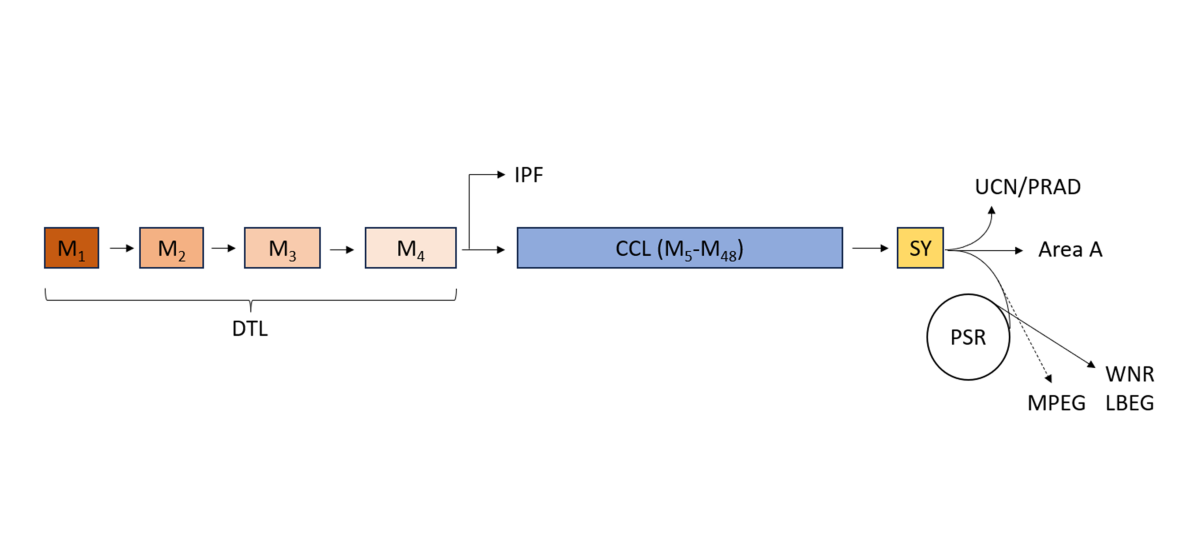
The LANSCE accelerator provides high-intensity $H^{+}$ and $H^{-}$ particle beams up to 800 MeV for various scientific experiments. A layout of the LANSCE linear accelerator is shown in Fig. 1. The LANSCE accelerator includes H+ and H- injectors, each featuring an ion source and a Cockcroft–Walton accelerator, to produce a 750 KeV beam. A beam transport system focuses, guides, and bunches the beams. Then, the 201.25-MHz Drift Tube linac (4 modules) accelerates the beam to 100 MEV, followed by a 805 MHz coupled-cavity linac (additional 44 modules) to accelerate the beams to 800 MeV. The beam is then used for applications in areas such as ultracold neutron source (UCN) studies, proton radiography (PRAD) for dynamic material imaging, and high-energy physics experiments. Additionally, beams can be directed to the proton storage ring (PSR) for creating highly intense beam bunches, used in the weapons neutron research (WNR) facility or the Lujan center for neutron scattering [59].

HPSim contains a realistic representation of the true beam used at LANSCE, able to simulate the beam as it passes through 48 modules of the Drift Tube Linac DTL and the Coupled Cavity Linac CCL. Each module includes two RF settings: one for controlling the phase of the electromagnetic wave responsible for beam acceleration, and another for adjusting the beam’s amplitude. To collect data from HPSim, first, the RF set points (amplitude and phase) for the first four modules are randomly sampled from a uniform distribution keeping the rest of the set points of 44 modules at a mean value. The sampled 96 dimensional vector is entered into the HPSim to simulate the beam dynamics across the length of the accelerator. We take the raw 6D HPSim output and project the particles to 15 unique projections ($x-p_{x}$, $x-y$, $x-p_{y}$, $x-z$, $x-p_{z}$, $y-p_{x}$, $y-p_{y}$, $y-z$, $y-p_{z}$, $z-p_{x}$, $z-p_{y}$, $z-p_{z}$ ($E-\phi$), $p_{x}-p_{y}$, $p_{x}-p_{z}$, and $p_{z}-p_{y}$) at each of the 48 modules.

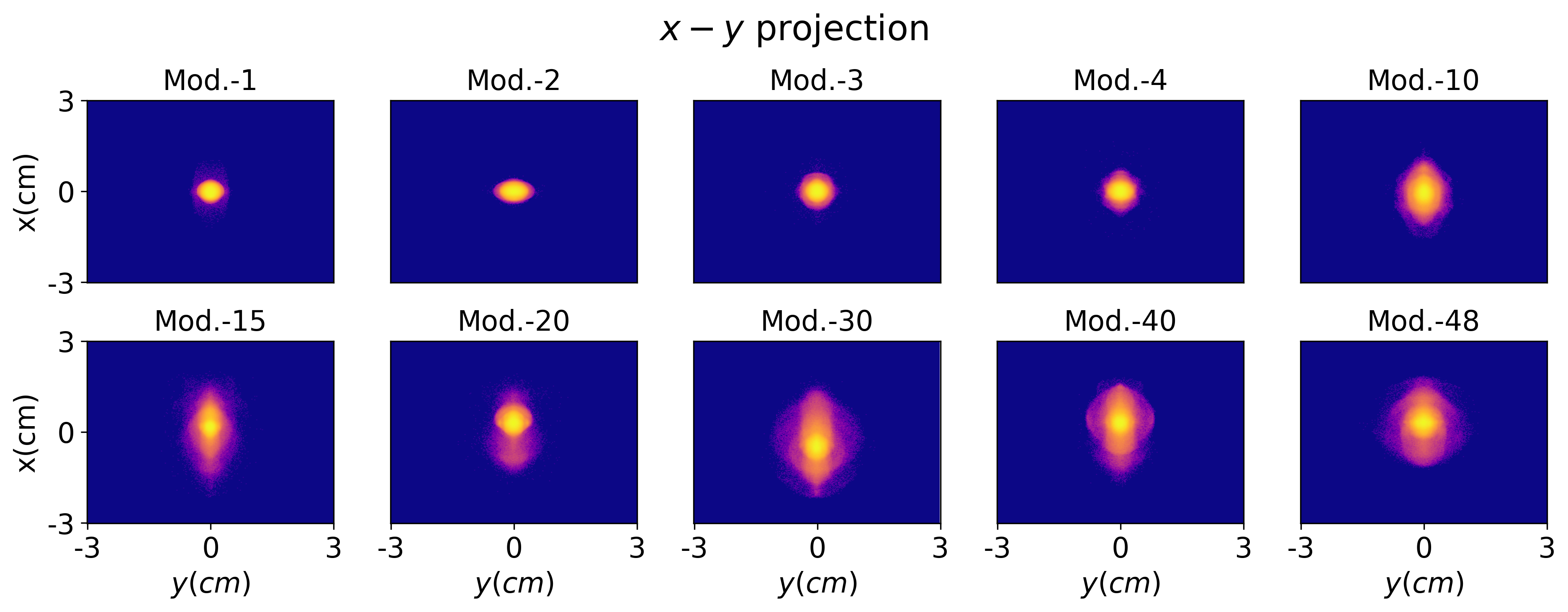
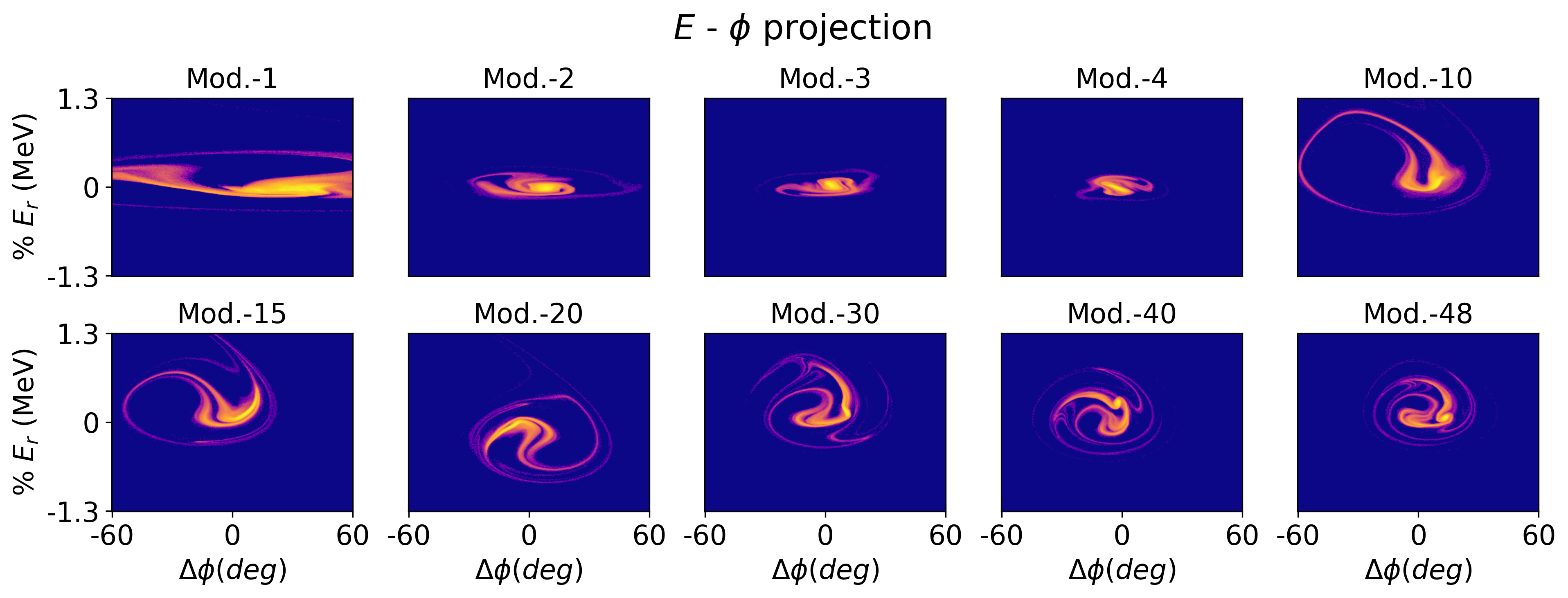
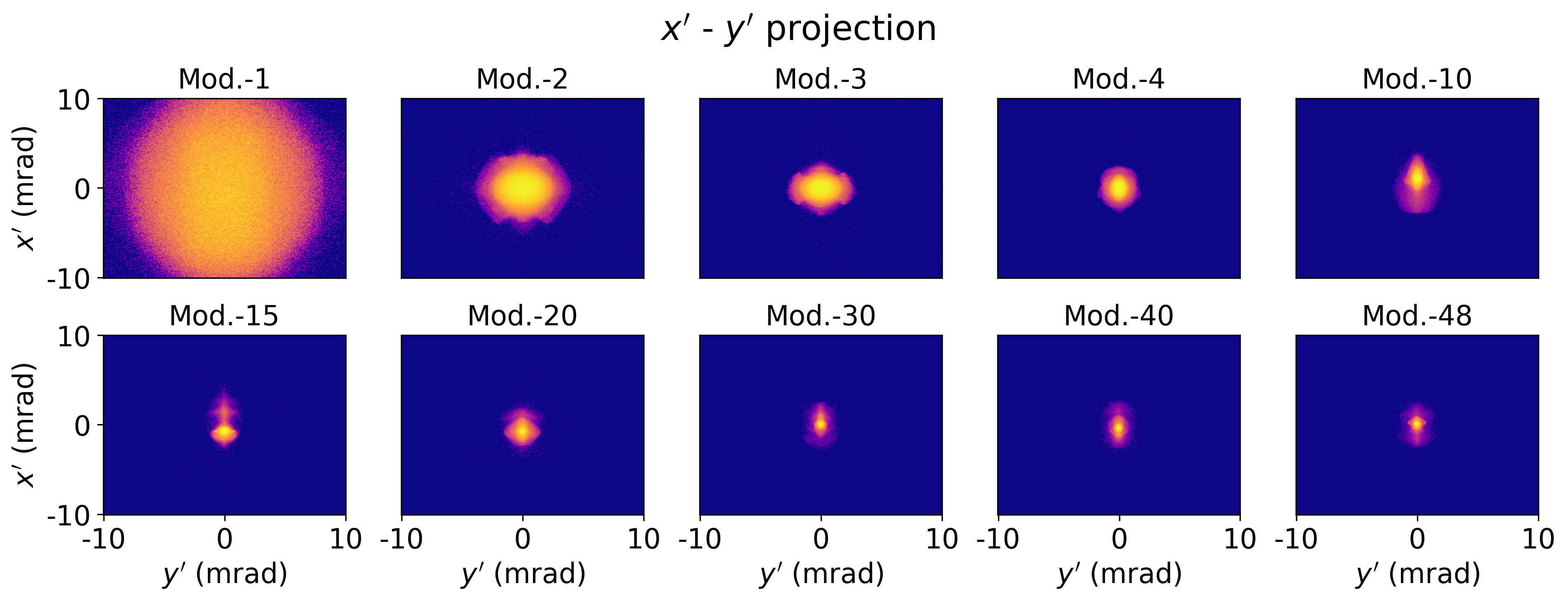
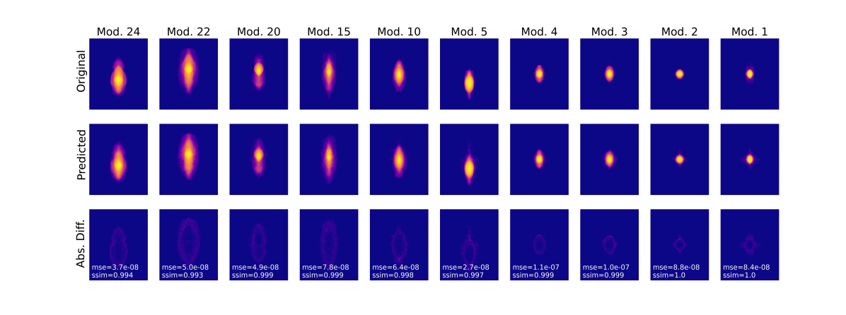
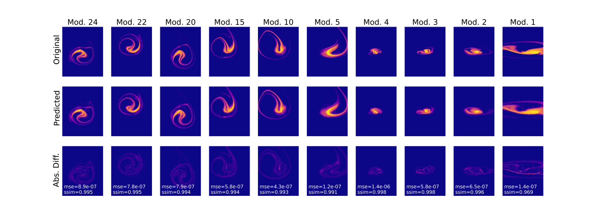
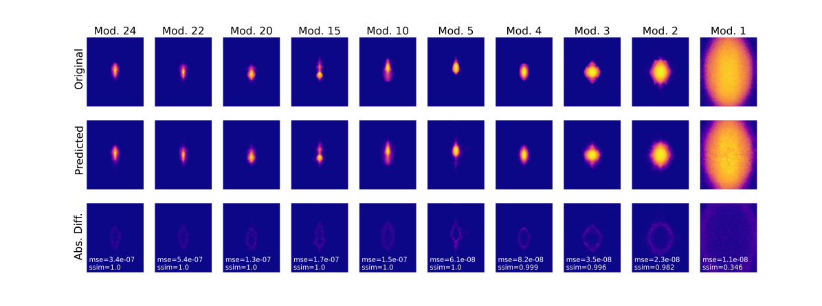
We have performed 1400 and 500 different simulations in the HPSim to collect the training and the test set, respectively. 3 out of 15 phase space projections ($x-y$, $E-\phi$, and $x^{\prime}-y^{\prime}$) for one of the simulation is plotted in Fig. 1. The plots are transformed to a logarithmic scale to compress the wide range of pixel intensity levels into a more compact range, enhancing visualization clarity. The projections evolve as they interact with RF electromagnetic fields while traversing various modules. Greater variations in projections are observed in the earlier modules, with the variations gradually decreasing as the beam progresses through the later modules.

Figure 1: A layout of the LANSCE linear accelerator and the related scientific areas like IPF, UCN/PRAD, WNR, Lujan, Area A, PSR. HPSim gives realistic representation of the true beam used at LANSCE. Three out of fifteen projections ($x-y$, $E-\phi$, $x^{\prime}-y^{\prime}$) of the 6D phase space of charged particle beams are shown at different modules.

2.3 Reverse latent evolution model

The beam dynamics described by Eqs. 1, 2 encodes evolution of a charged particle beam’s phase space density $\rho$ in the forward time direction. For notational simplicity we refer to $\rho$ at different times as $\{\rho_{1},\rho_{2},\dots,\rho_{M}\}$, where $M$ is the final accelerating module. Since we are working with the phase space of charged particles denoted as $X$ rather than phase space density $\rho$, we adopt notations using $X$ instead of $\rho$. The LANSCE accelerator has 48 different accelerating modules, therefore, the temporal discretization or time steps becomes 48 ($X_{1},X_{2},\dots,X_{48}$).

The forward discretized spatiotemporal beam dynamics problem can be written as $X_{m}=H(X_{1},X_{2},...,X_{m-1})$, where $H$ is a unknown nonlinear function that can be learned as $P(X_{M}|X_{1},X_{2},...,X_{M-1})$ with a latent evolution model [18]. Reversing the temporal dynamics to predict the current state $X_{m}$ given future states $X_{m+1},X_{m+2},\dots,X_{M}$, requires inverting the function $H$, which becomes a challenging inverse problem. Additionally, the time-varying nature of RF parameters and initial distribution further complicates the problem. The inverse problem can be learned by calculating the joint probability distribution $P(X_{1},X_{2},...,X_{M})$. This distribution can be computed with a reverse autoregression, where $P(X_{1},X_{2},...,X_{M})$ is factored as $P(X_{M})P(X_{M-1}|X_{M})P(X_{M-2}|X_{M-1},X_{M})$ ….
$P(X_{m}|X_{m+1},X_{m+2},\dots,X_{M})$.

For particle accelerators, $X$ is a high-dimensional object comprising positions and momentum of billions of particles. Learning such a high-dimensional probability distribution and calculating $P(X_{m}|X_{m+1},X_{m+2},\dots,X_{M})$ to estimate $X_{m}$ at any given module is computationally challenging. Fortunately, latent variable models (like variational autoencoders) transform the higher-dimensional distribution $P(X_{1},X_{2},...,X_{M})$ into a lower-dimensional distribution $P(\mathbf{z}_{1},\mathbf{z}_{2},...,\mathbf{z}_{M})$ using Bayesian inference [60]. The reverse autoregressive approach can then be applied to this lower-dimensional distribution, calculating $P(z_{m}|z_{m+1},z_{m+2},\dots,z_{M})$ to estimate $\mathbf{z}_{m}$. A recurrent neural network (RNN) like an LSTM can be used to invert the forward temporal dynamics in the latent space. The LSTM needs to be trained autoregressively to learn $\mathbf{z}_{m}=G(\mathbf{z}_{m-1:M})$ for all $m$, where $G$ is the combined functional relationships of LSTM [61]. This can be accomplished by training the LSTM with a variable input size. Once the inverse temporal dynamics is learned in the latent space, the decoder part of the VAE transforms it back to the high-dimensional space, obtaining $P(X_{m}|X_{m+1},X_{m+2},\dots,X_{M})$.

The autoregressive procedure used to train the LSTM is a crucial aspect of rLEM. It is a general formulation which does not assume a strict Markov property, i.e. $P(z_{m}|z_{m+1},z_{m+2},\dots,z_{M})=P(z_{m}|z_{m+1})$, on the temporal dynamics. Since the temporal dynamics are learned in a lower-dimensional latent space rather than the higher-dimensional image space ($n_{d}\approx 10^{6}$), $M$-step autoregression compensates for the information loss due to spatial dimensionality reduction. A single step autoregression model, using $P(z_{m}|z_{m+1})$, suffers in performance compared to the $M$-step autoregressive model. Additionally, autoregression procedure leverages temporal periodicity (short-term or long-term seasonality) present in the dataset better than Markov property.

The reverse latent evolution approach described above combines a conditional variational autoencoder (CVAE) to project the 15 unique projections of the 6D phase space of charged particle beams into a lower-dimensional latent distribution. Subsequently, a LSTM network learns the reverse temporal dynamics within this latent space. During the prediction stage, both networks are integrated into an autoregressive loop to estimate all the upstream phase space projections given limited downstream measurements. The architecture of the rLEM is represented in Fig. 2. The model learns spatial and temporal correlations independently in two-step self-supervised process. The encoder performs convolution operations to extract features from the images. The module number is passed through dense layers and concatenated with the features vectors out of the encoder. The concatenated vector is the input to the latent space. The LSTM network operates on the learned latent space to predict the previous latent space points (corresponding to projections in the upstream modules) based on future points (corresponding to projections in the downstream modules). The predicted latent points are passed through a decoder which generates phase space projections across different modules of the accelerator.

Figure 2: Reverse latent evolution model (rLEM): CVAE captures a lower-dimensional latent distribution of a higher-dimensional 6D phase space followed by an autoregressive LSTM learning to reverse temporal dynamics in the latent space.

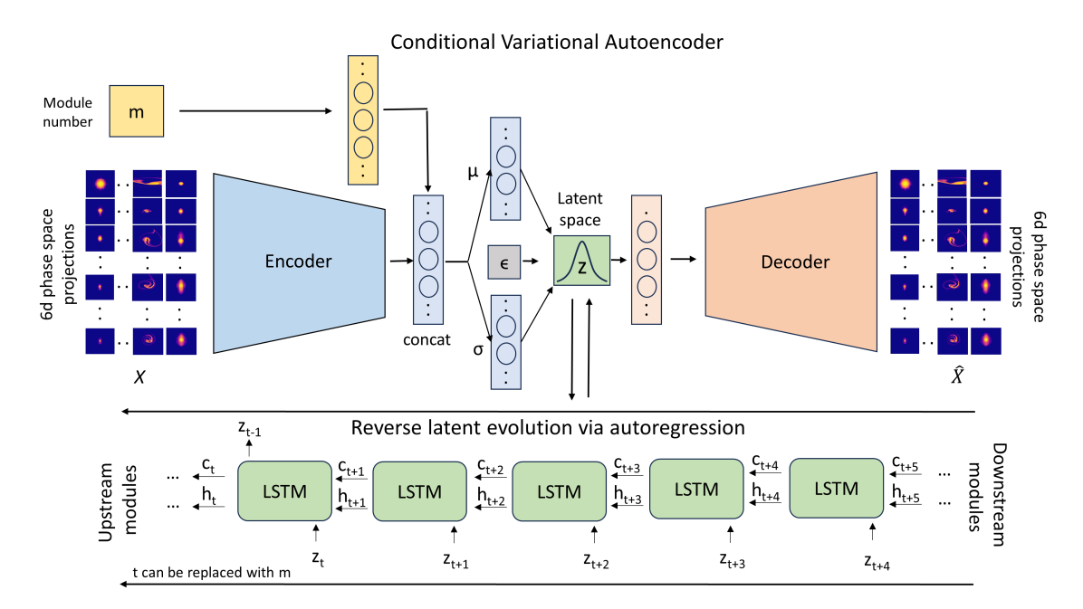
A mathematical description of the working of the rLEM algorithm can be written in terms of the CVAE and LSTM, combined through latent space $\mathbf{z}$. The posterior distribution $p_{\theta}(\mathbf{z}|\mathbf{x},m)$ (conditioned on the the module number in our work) can be written using Bayes rule:

$$p_{\theta}(\mathbf{z}|\mathbf{x},m)=\frac{p_{\theta}(\mathbf{x}|\mathbf{z},m)p_{\theta}(\mathbf{z}|m)p_{\theta}(m)}{p_{\theta}(\mathbf{x})}.$$ (4)

The above posterior is intractable and cannot be solved. CVAE introduces a parameterized distribution $q_{\phi}(\mathbf{z}|\mathbf{x},m)$ to reduce the dimensionality of the problem. It is an inference model that maps data $\mathbf{x}$ to the latent space $\mathbf{z}$ by approximating the posterior distribution $p_{\theta}(\mathbf{z}|\mathbf{x},m)$. Since, $p_{\theta}(m)$ is known and provides $p_{\theta}(\mathbf{z}|m)$, therefore, $p_{\theta}(\mathbf{x}|\mathbf{z},m)=p_{\theta}(\mathbf{x}|\mathbf{z})$. The loss function can be written in the form of Evidence Lower BOund (ELBO) [62]:

$$ELBO(\theta,\phi;\mathbf{x}) = \mathbb{E}_{\mathbf{z}\sim q_{\phi}(\mathbf{z}|\mathbf{x},m)}[\log p_{\theta}(\mathbf{x}|\mathbf{z})]$$

$$-D_{KL}(q_{\phi}(\mathbf{z}|\mathbf{x},m)||p_{\theta}(\mathbf{z}|m)).$$

In ELBO, the first term represents the reconstruction loss between the original and the predicted data whereas the second term is the Kullback–Leibler (KL) divergence between the posterior distribution and the approximate posterior [63].

An LSTM is employed as a backcasting model to predict previous states (upstream modules) of the latent space based on limited downstream states. The LSTM equations [64], originally expressed in terms of input $x_{t}$ and output $y_{t}$ at time $t$, are reformulated to backcast $\mathbf{z}_{m-1}$ (output) given $\mathbf{z}_{m}$ (input), with $m$ denoting the module number:

$$i_{m}=\sigma(W_{ii}\mathbf{z}_{m}+b_{ii}+W_{hi}h_{m+1}+b_{hi})$$ (5)

$$f_{m}=\sigma(W_{if}\mathbf{z}_{m}+b_{if}+W_{hf}h_{m+1}+b_{hf})$$ (6)

$$g_{m}=\tanh(W_{ig}\mathbf{z}_{m}+b_{ig}+W_{hg}h_{m+1}+b_{hg})$$ (7)

$$o_{m}=\sigma(W_{io}\mathbf{z}_{m}+b_{io}+W_{ho}h_{m+1}+b_{ho})$$ (8)

$$c_{m}=f_{m}\odot c_{m+1}+i_{m}\odot g_{m}$$ (9)

$$h_{m}=o_{m}\odot\tanh(c_{m})$$ (10)

$$\mathbf{z}_{m-1}=\sigma(W_{hy}h_{m}+b_{hy})$$ (11)

where, $h_{m}$, $c_{m}$, $\mathbf{z}_{m}$ are the hidden state, cell state and input at module $m$. $i_{m}$, $f_{m}$, $g_{m}$, $o_{m}$ are respectively the input, forget gate, cell and output gates. $h_{m+1}$ is the hidden state at module $m+1$. $\sigma$ is the logistic sigmoid activation and $\odot$ is the Hadamard product. $W$ and $b$ are respective weights and bias matrices. A mean squared error-based loss function is used between true $\mathbf{z}_{m}$ and predicted $\hat{\mathbf{z}}_{m}$ values of latent point at module $m$.

$$MSE=L(\psi;\mathbf{z})=\parallel\mathbf{z}_{m}-\hat{\mathbf{z}}_{m}\parallel_{2}$$ (12)

The aforementioned equations are simplified with single input and single output but can be written multiple inputs and a single output.

During the prediction phase, the trained CVAE and LSTM are integrated in an autoregressive loop to facilitate the predictions of phase space projections in upstream modules. The methodology is outlined in Algorithm 1. The input of the algorithm is the user-defined phase space at downstream location of the measurement ($m_{end}$) and the upstream module until where phase space predictions are desired, denoted by $m_{start}$. Typically, $m_{start}$ is set to 1, corresponding to the index of the first module, but it can also be any other module number $<m_{end}$. $m_{end}$ can be a single module, or multiple modules together. For the first iteration, the encoder of CVAE projects $X_{M:m}$ into the latent space to obtain $\mathbf{z}_{M:m}$. Subsequent iterations use only the LSTM and decoder of the CVAE. The LSTM acts on the latent representation to predict $\mathbf{z}_{m-1}$. The decoder of the CVAE then reconstructs $X_{m-1}$, providing the phase space projections at the previous module. The predicted latent point $\mathbf{z}_{m-1}$ is then concatenated with input $\mathbf{z}_{M:m}$ to form $\mathbf{z}_{M:m-1}$. This autoregressive procedure is iteratively applied to compute $\mathbf{z}_{m-2}$, followed by $X_{m-2}$, and so forth, until $m_{start}$.

Algorithm 1 rLEM prediction algorithm

1:Input: $m_{start}$, $m_{end}$, trained CVAE, trained LSTM

2:for $m$ = $m_{end}$ $\rightarrow$ $m_{start}$ do

3:     if $m$ = $m_{end}$ then

4:         $\mathbf{z}_{M:m}$ = CVAE-encoder($X_{M:m}$, $M:m$)      

5:     $\mathbf{z}_{m-1}$ = LSTM($\mathbf{z}_{M:m}$)

6:     $X_{m-1}$ = CVAE-decoder($\mathbf{z}_{m-1}$)

7:     $\mathbf{z}_{M:m-1}$ = concat($\mathbf{z}_{M:m}$, $\mathbf{z}_{m-1}$)

3 Results and Discussion

We have collected 1400 training data samples and 500 test data samples by running HPSim for different random RF settings. Every sample contains 15 unique phase space projections are depicted as 15 channels, each represented by a 256 $\times$ 256 pixel image along the 48 modules of the accelerator. The entire data set has size 1400 × 48 × 15 × 256 × 256 . The conditional input m to the encoder is the module number, a scalar between 1-48, normalized to the range [0, 1].

The dataset comprising 1400 data objects is partitioned into training and validation sets with an 85:15 ratio. The encoder of the CVAE is composed of five convolutional layers with 32, 64, 128, 256, and 512 filters of size 3×3, each with a stride of 2, followed by a dense layer with 256 neurons. Additionally, a separate dense branch processes the module number through two layers of 32 neurons. The outputs of the primary and branch layers are concatenated and fed into the latent dense layer. We have performed a trial-and-error study balancing dimensions and loss to select the dimensionality of the latent space. This lower-dimensional representation enhances interpretability and reduces training time. The decoder mirrors the encoder’s architecture, featuring a dense layer followed by convolutional layers with 512, 256, 128, 64, and 32 filters of size 3×3. Each layer employs the LeakyReLU activation function and batch normalization.

The CVAE network is optimized using the Adam optimizer with a learning rate of 0.001 and a batch size of 32, over 1500 epochs. This configuration proved effective in balancing performance and efficiency.

3.1 Latent space visualizations

Figure 3: Latent space visualization: Top row shows 7 2d projections ($Z_{1}-Z_{2:7}$) of 8d latent space. The bottom row shows 2D PCA and 2D t-SNE of the 8D latent space. The first two figures in the row shows train-test points and the last two figures shows combined train-test colored based on 48 modules.

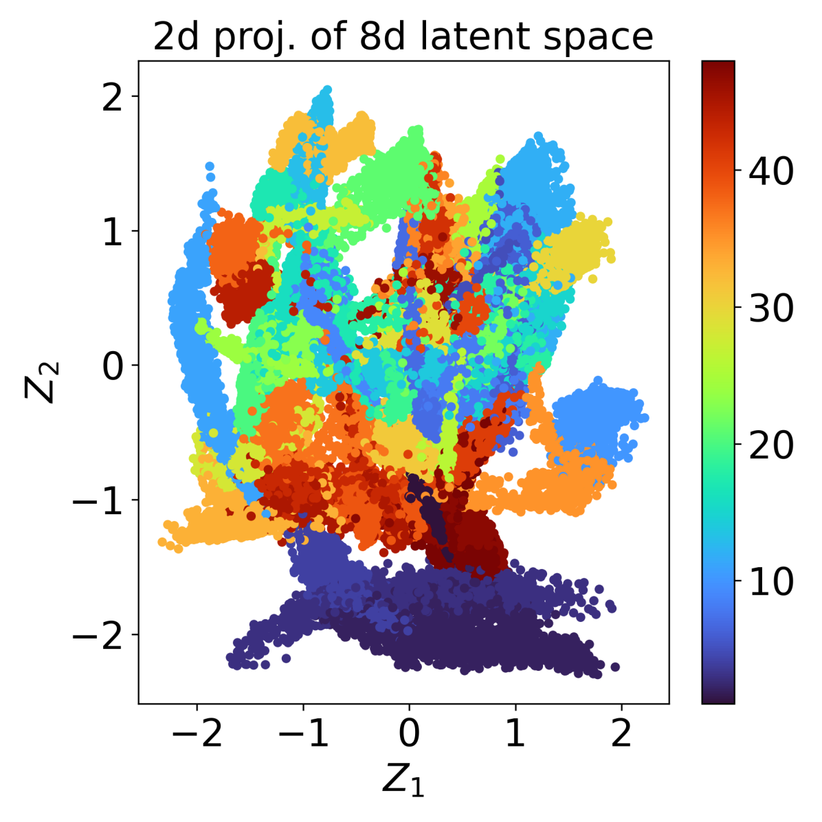
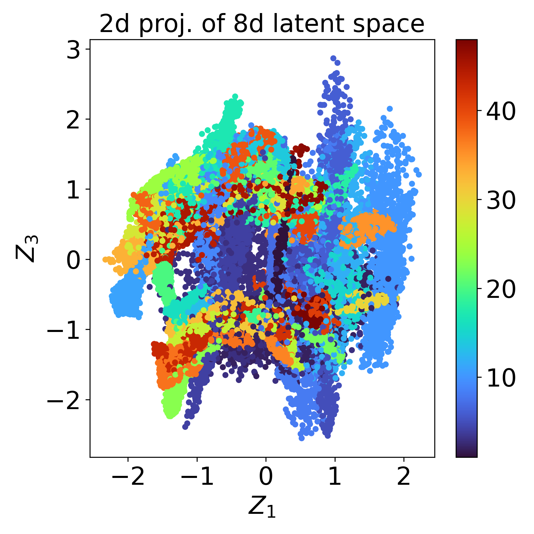
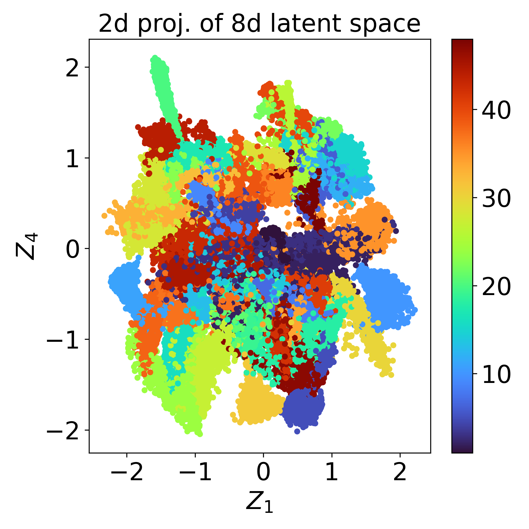
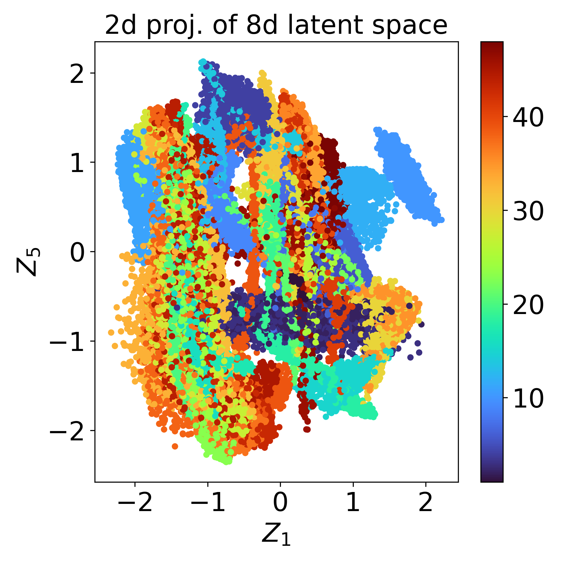
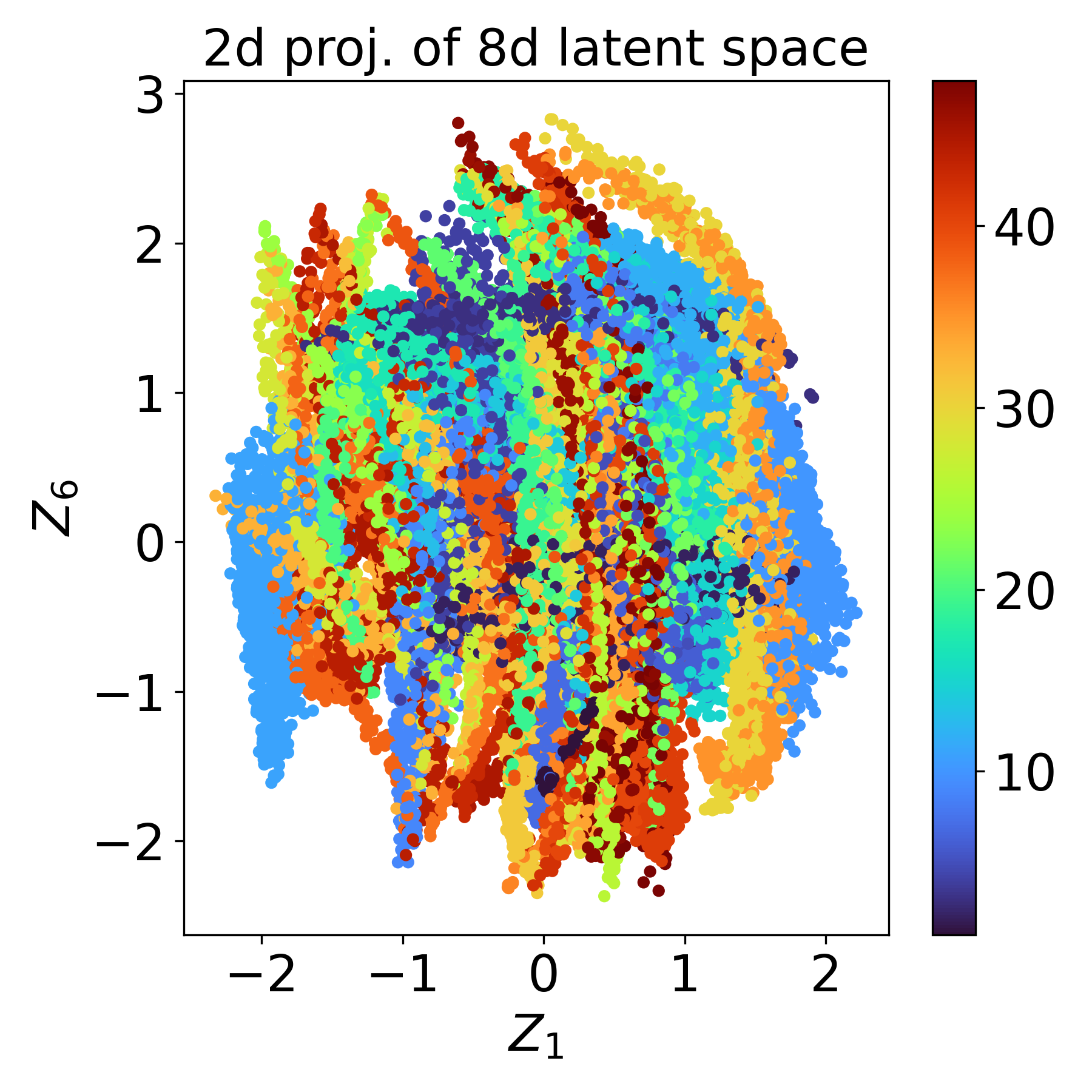
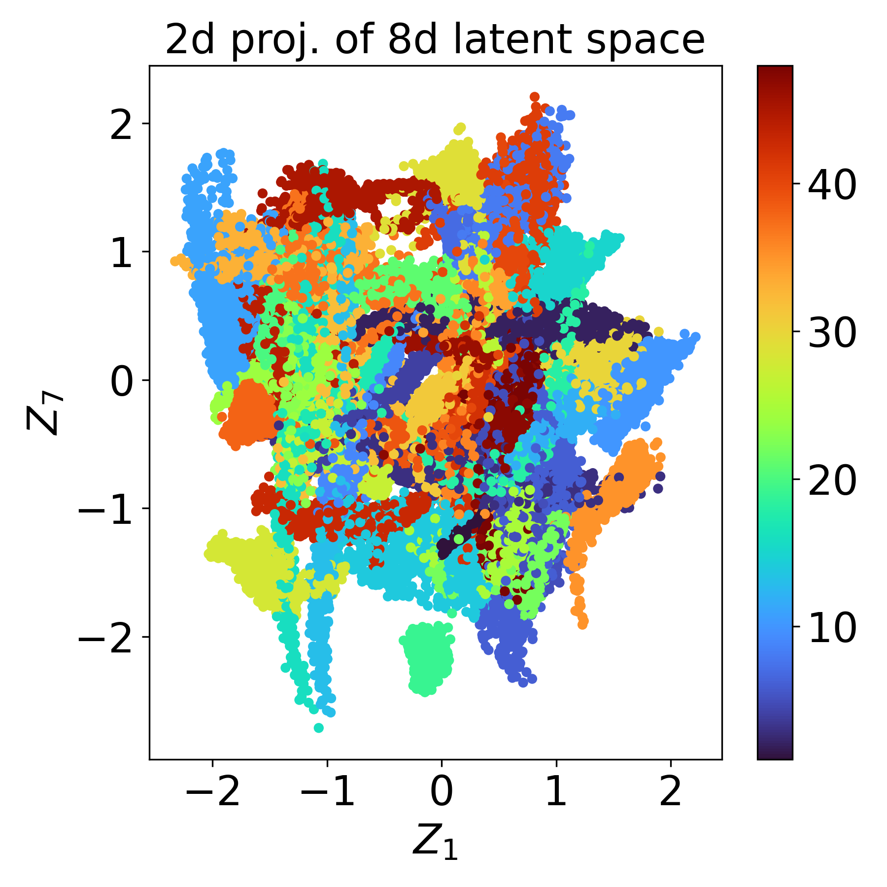
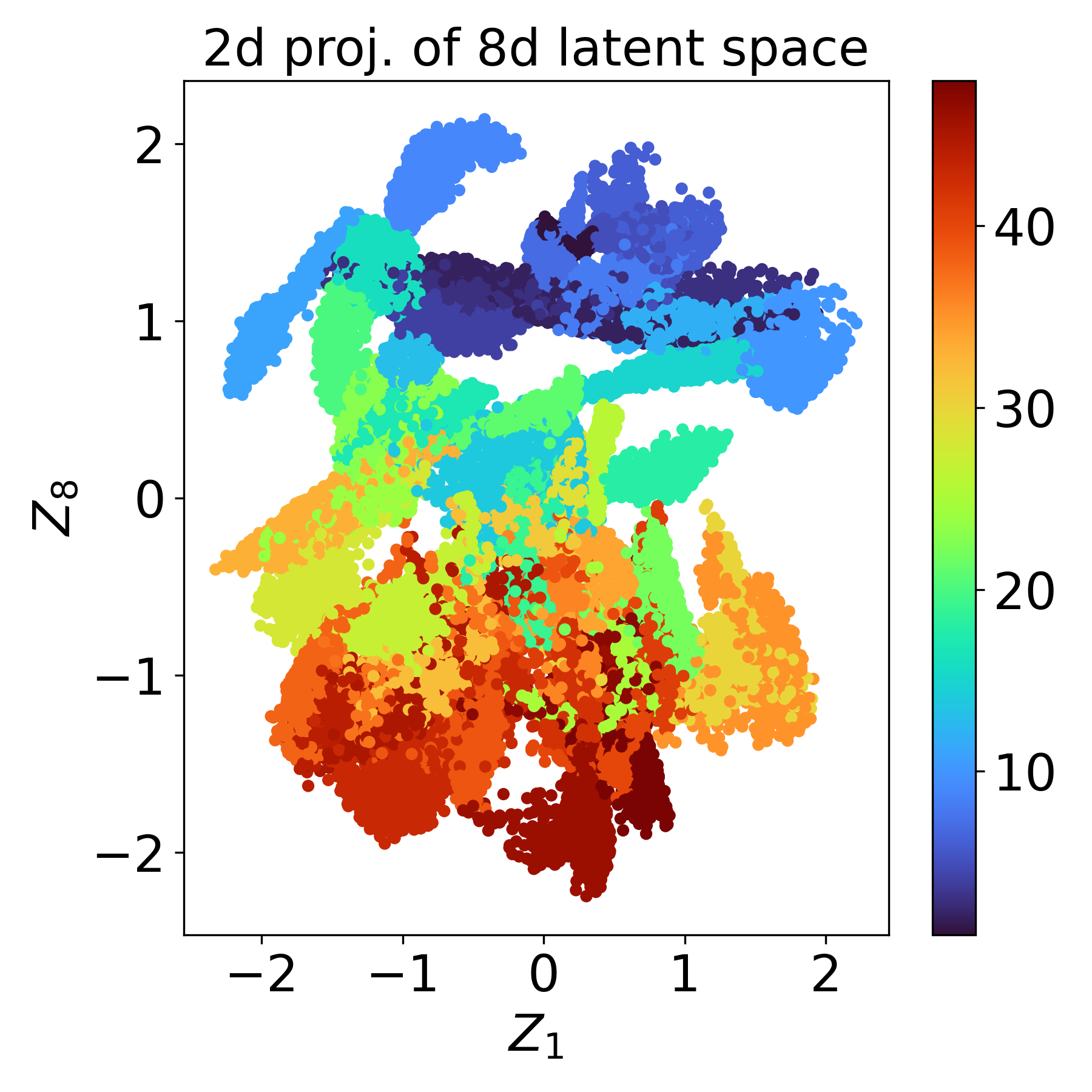
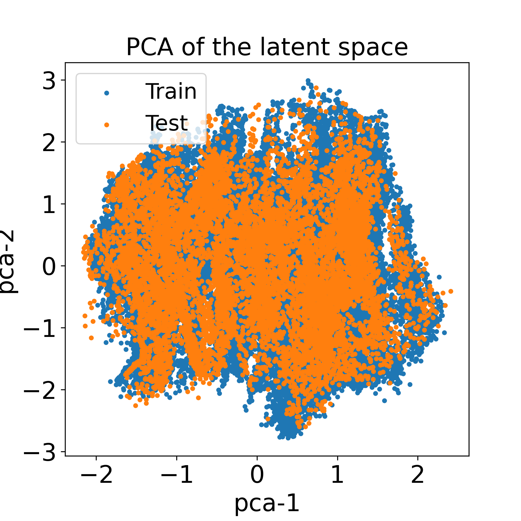
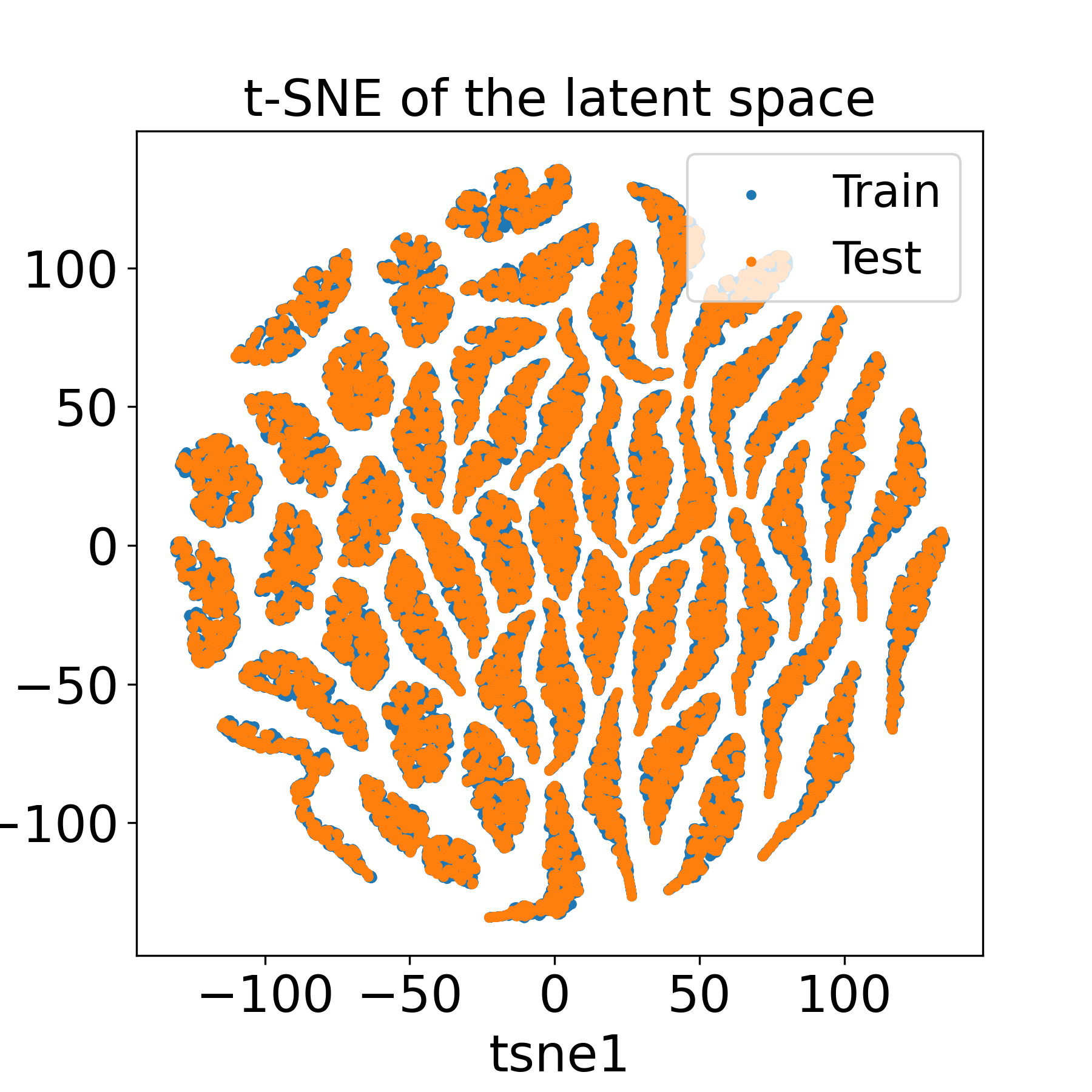
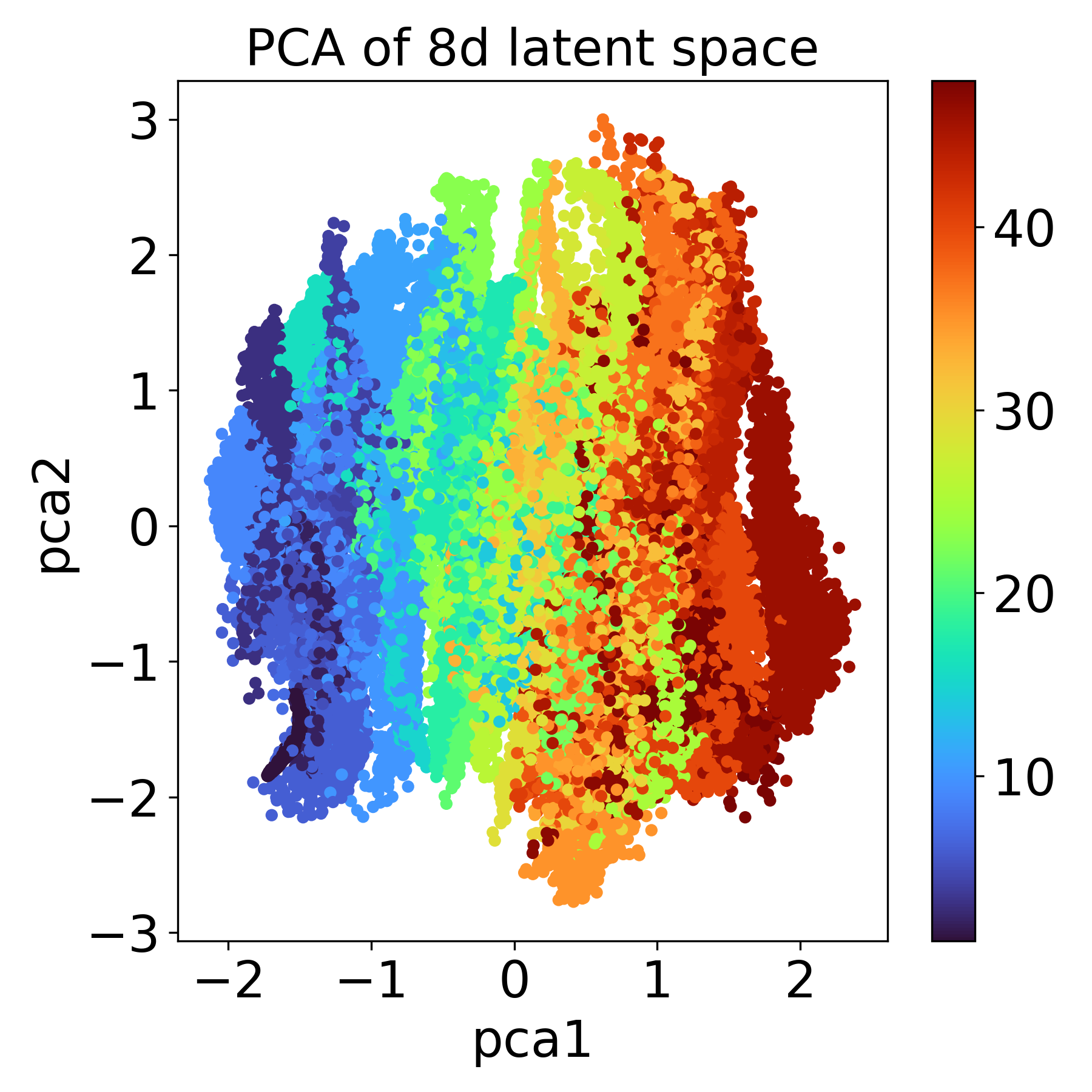
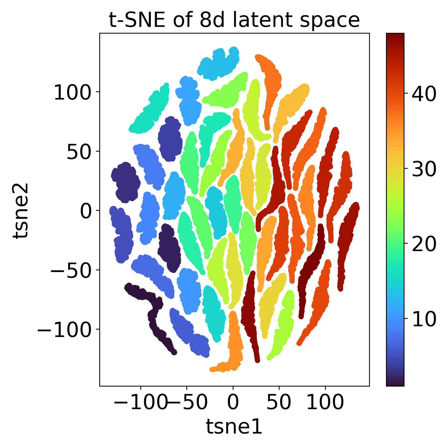
The latent space of a VAE naturally lead to continuous latent space representations that can be smoothly traversed, making them well suited for probabilistic density estimation and generation [65]. Visualization of the latent space is important because it offers valuable insights into the extracted features, which eventually enhances the network’s interpretability. Seven 2D projections of the the 8D latent space is plotted in the top row of Fig. 3. It can be observed from the 2D projection of the latent space that the phase space in different modules are much more separated in $Z_{1}-Z_{8}$ than $Z_{1}-Z_{2}$, and $Z_{1}-Z_{4}$ and $Z_{1}-Z_{5}$ projections. But, visualizing remaining 2D projections is still cumbersome even with 8D latent space.

We have transformed 8D latent space into 2D space using two of the most popular dimensionality reduction techniques i.e. principal component analysis (PCA) and t-stochastic nearest neighbors (t-SNE) [66]. PCA is a linear reduction technique, whereas t-SNE is a non-linear manifold learning approach. PCA and t-SNE of the 8D latent space is shown in Fig. 3. The first two plots in the bottom row shows the location of the points corresponding to the training and test set in PCA and t-SNE space. The last two plots show PCA and t-SNE space color coded with different modules.

It is seen from the PCA plot that the points belonging to the initial and end modules are well separated, with a gradual variation in modules as we move along the PCA space. In t-SNE space, similar to PCA, the initial and end modules occupy different ends of the space. It is easily noticeable that there is better separation of different modules into clusters in the t-SNE space. This is to be expected as PCA is a linear method with limited expressive power as compared to nonlinear t-SNE method. Also, PCA is formulated to project high-dimensional data into principal space by maximizing the variance of the data. On the other hand, t-SNE is designed for clustering of points in the lower dimensional space.

The ability to distinguish phase space projections in various modules at different positions demonstrates that the CVAE has effectively learned the spatial correlations of phase space projections across different modules.

3.2 Prediction results

For training LSTM, the latent space of trained CVAE is reshaped from 67,200$\times$8 to 1400$\times$48$\times$8, where 1400 signifies the number of samples, 48 denotes the total number of modules, and 8 is the dimension of the latent space. In LSTM terminology, 48 becomes the trajectory length and 8 are number of features. In order for autoregressive prediction, the LSTM is trained with variable-length inputs and single-length output. The 8D trajectory with length 48 is split using input window of sizes varying from 1 to 47 and output window of size of 1. The two windows slides on the 8D trajectory from right to left to split it into different input sizes varying from $1\times 8$, $2\times 8$, …, $47\times 8$, while the output remains fixed at ${1\times 8}$ (representing the upstream module). The variable-length trajectories are made compatible with the LSTM by padding them with zeros to achieve a uniform length of 47. However, the LSTM masks these padded zeros while learning the temporal dynamics through recurrence.

The LSTM training with variable-length input and a single output allows the network to learn the autoregressive temporal patterns of the latent points, which is essential for making autoregressive predictions in the latent space. Our LSTM architecture comprises two layers, each with 64 hidden units. We minimize the mean squared error (MSE) between the true and predicted latent vectors, as defined in Eq. 12, using an Adam optimizer. The initial learning rate is set to 0.001 and is halved after 10 epochs if the validation loss plateaus.

A trained rLEM network can be used to autoregressively predict upstream phase space projections based on downstream phase space projections provided as inputs. The prediction procedure is detailed in Algorithm 1 and explained in Sec. 2.3. The algorithm operates with a user-defined downstream location (input) where the measurement is specified and the number of upstream locations where predictions are needed (output). It is flexible regarding inputs, accommodating multiple consecutive or non-consecutive downstream locations. Depending on the inputs, it can provide phase space projections for single, multiple, consecutive, or non-consecutive upstream locations.

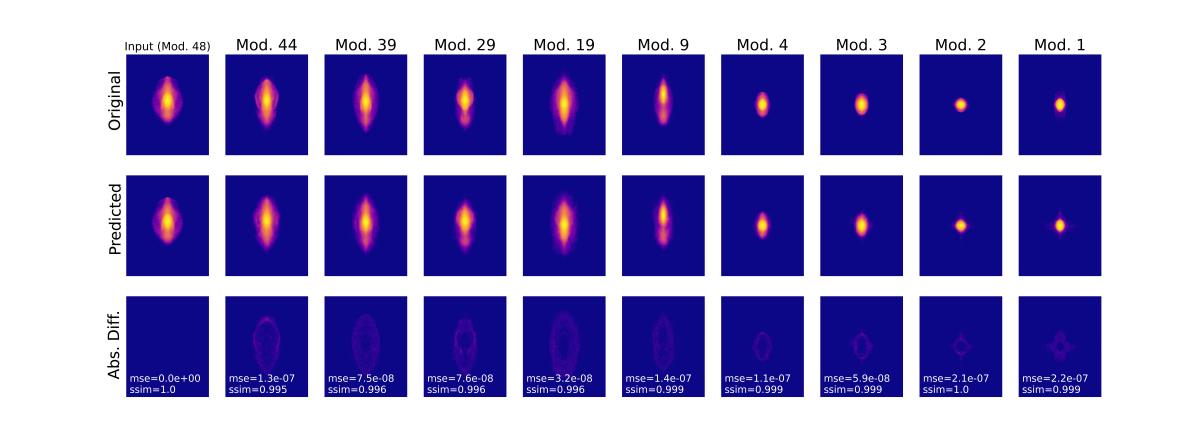
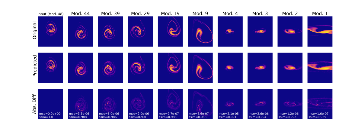
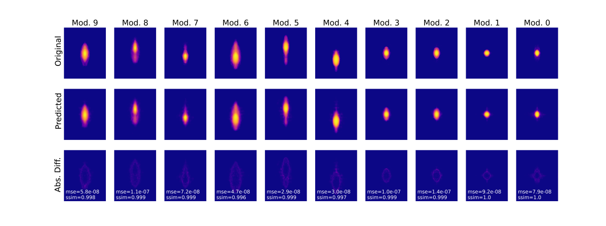
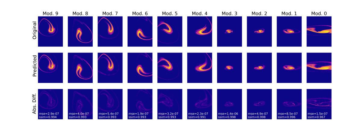
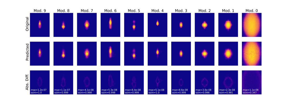
Fig. 4 shows prediction in all the upstream modules given the last module (module 48) as the input. Similar plots using module 10 and module 25 as inputs are shown in Figs. A.3 and A.4. For brevity, three out of fifteen projections are shown across nine different modules. The original and predicted images can be compared using absolute difference plots. The mean squared error (MSE) and structural similarity index (SSIM) are also calculated and displayed alongside the absolute difference plots. It is evident from the figures and comparison metrics that rLEM performs well, demonstrating high accuracy prediction capabilities. We achieve an overall MSE and SSIM of ($\approx$ 5e-7, $\approx$ 0.998) and ($\approx$ 1e-6, $\approx$ 0.976) on the training and test set.

(a) $x-y$ projection

(b) $E-\phi$ projection

(c) $x^{\prime}-y^{\prime}$ projection

Figure 4: Predictions from the trained rLEM at different upstream modules given module 48 as the input. The original, predicted and the absolute difference are plotted for (a) $x-y$ projection, (b) $E-\phi$ projection and (c) $x^{\prime}-y^{\prime}$ projection across nine different modules.

In this work we are only modifying the RF parameters of the first 4 RF modules of LANSCE which comprise the initial 201.25 MHz section of the accelerator. The quadrupole magnetic lattice and the 44 subsequent RF cavities of the 805 MHz section of the accelerator are unchanged and their limited beam acceptance acts as a powerful screening mechanism so that the variance of the beams which do survive to the end of the accelerator cannot be very large. In future work, we plan on adjusting the RF parameters of all 48 RF modules of LANSCE and of the magnetic lattice, which will allow for the survival (particles not being lost as they hit the walls of the accelerator beam pipe along the way) of a much more diverse set of beams to the end of the accelerator.

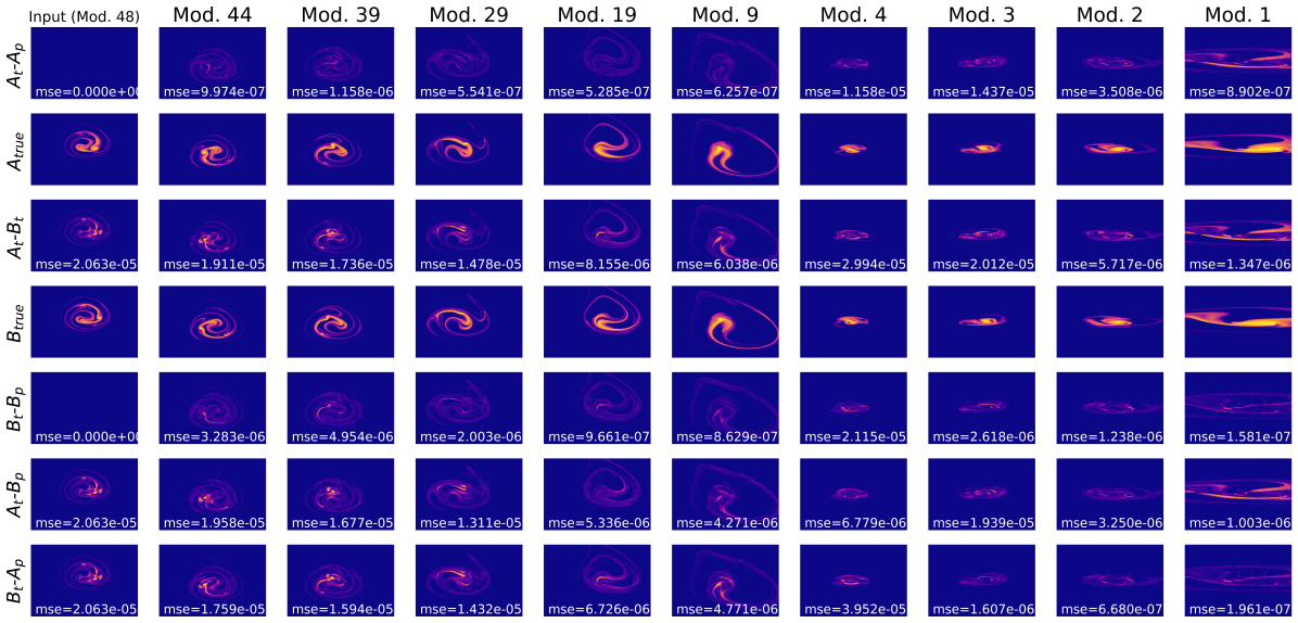
Despite the screening process of the accelerator, upon a detailed inspection one can see significant differences in the detailed phase space distributions of the various beams on our training and test sets, and these differences are easily quantified via metrics such as mean squared error (MSE). In order to clearly demonstrate the ability of the LSTM to distinguish between different beams, we show 2 examples in Fig. A.2 where we show two beam examples side by side ($A_{true}$ and $B_{true}$), their differences from each other at various modules ($A_{t}-B_{t}$), and their differences from the LSTM-based autoregressive predictions ($A_{t}-A_{p}$ and $B_{t}-B_{p}$). It is shown that the LSTM is able to accurately track them with a much lower MSE than the difference between the two beams, which is what would happen if one example was simply used as a guess attempting to predict the other.

Generating predictions for all 15 projections in all 47 modules takes less than one second with rLEM, whereas the simulator requires about 10 minutes on similar computing infrastructure. This results in a speedup factor of approximately 600.

3.3 Uncertainty analysis results

3.3.1 Aleatoric uncertainty in the latent space

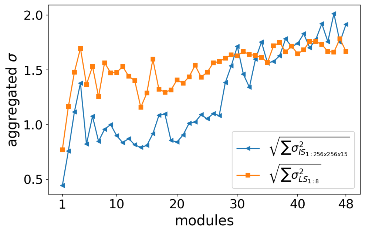
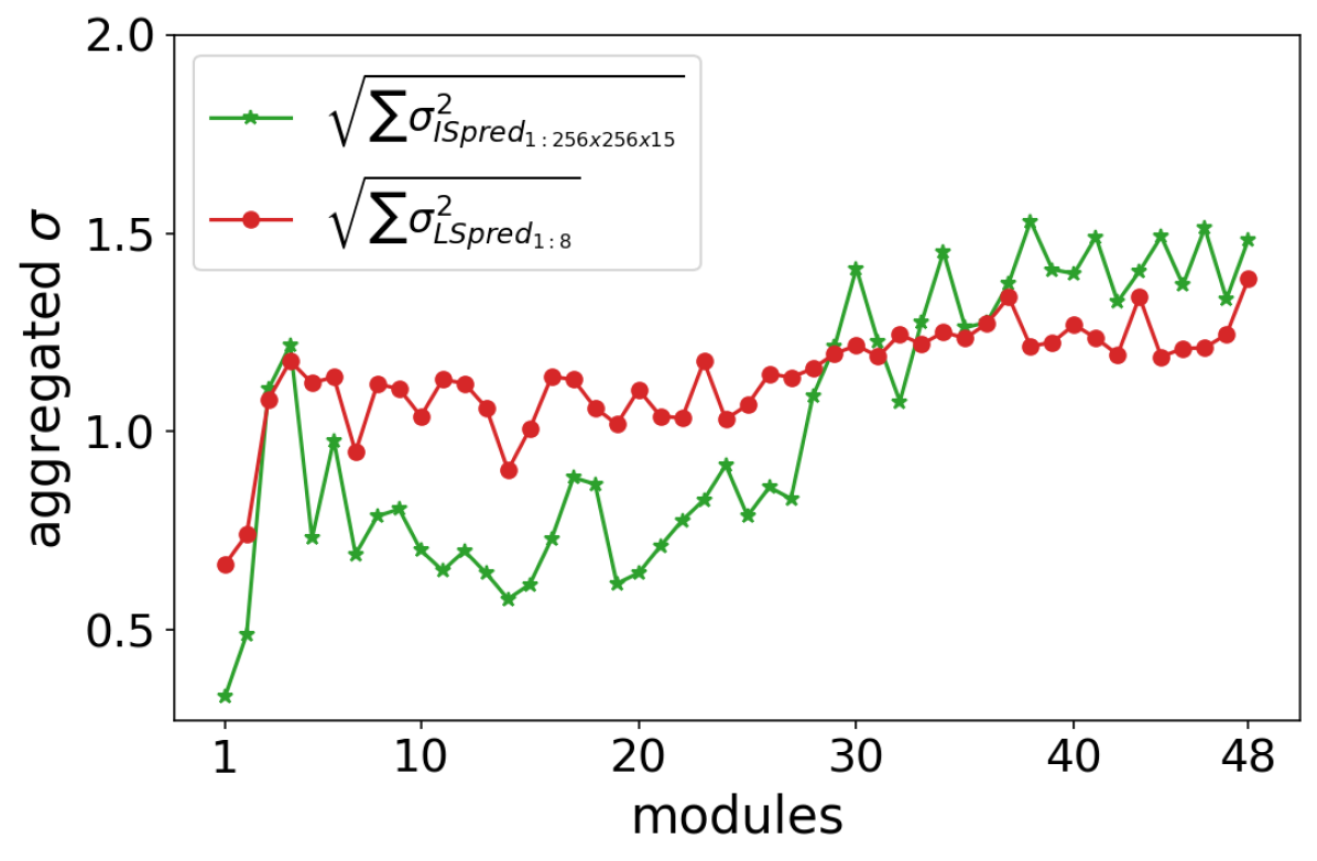
The VAE learns a lower-dimensional representation of images through a probabilistic density function, which can be randomly sampled and decoded to generate new, realistic in-distribution (ID) images [67]. This is possible because the VAE’s latent space encodes the aleatoric uncertainty of the higher-dimensional input dataset [68, 42]. To quantify this aleatoric uncertainty in the latent space, we collected 10,000 Monte-Carlo samples from all the modules by conditionally sampling the latent space within the bounds of the corresponding modules. The mean and standard deviation are calculated and presented in Fig. 5 for all eight dimensions of the latent space across all 48 modules. Notably, the standard deviation varies across different dimensions, being higher in the 4th and 5th dimensions. Additionally, we have plotted the aggregated standard deviation ($\sum{\sigma_{LS_{1:8}}^{2}}$) in Fig. 6(a), represented by the blue curve. The aggregated standard deviation, which measures the total spread across all dimensions, shows an increasing trend towards the later modules, purely due to the physical nature of the problem with data in later modules simply containing more variance. This is also evident with the orange curve, which demonstrates that the aggregated standard deviation in image space ($\sqrt{\sum{\sigma_{IS_{1:256x256x15}}^{2}}}$) follows a similar trend to that in latent space (LS). Although a direct comparison of relative differences is challenging due to the different ranges in image space and latent space, the overall trend remains clearly observable.

Figure 5: Latent space bounds for all the modules for all the 8 dimensions. The space is conditionally sampled 10k times at different modules followed by calculating the mean and standard deviation for every module and dimension.

Figure 6: Comparison of aggregated mean and standard deviation of (a) Dataset (Image space (IS): 1400x48x256x256x15) and latent space (LS) across different modules (10k MC samples in 48 modules) (b) LSTM based predictions of the upstream latent space (520 true trajectories) and corresponding decoded images (520x48x256x256x15).

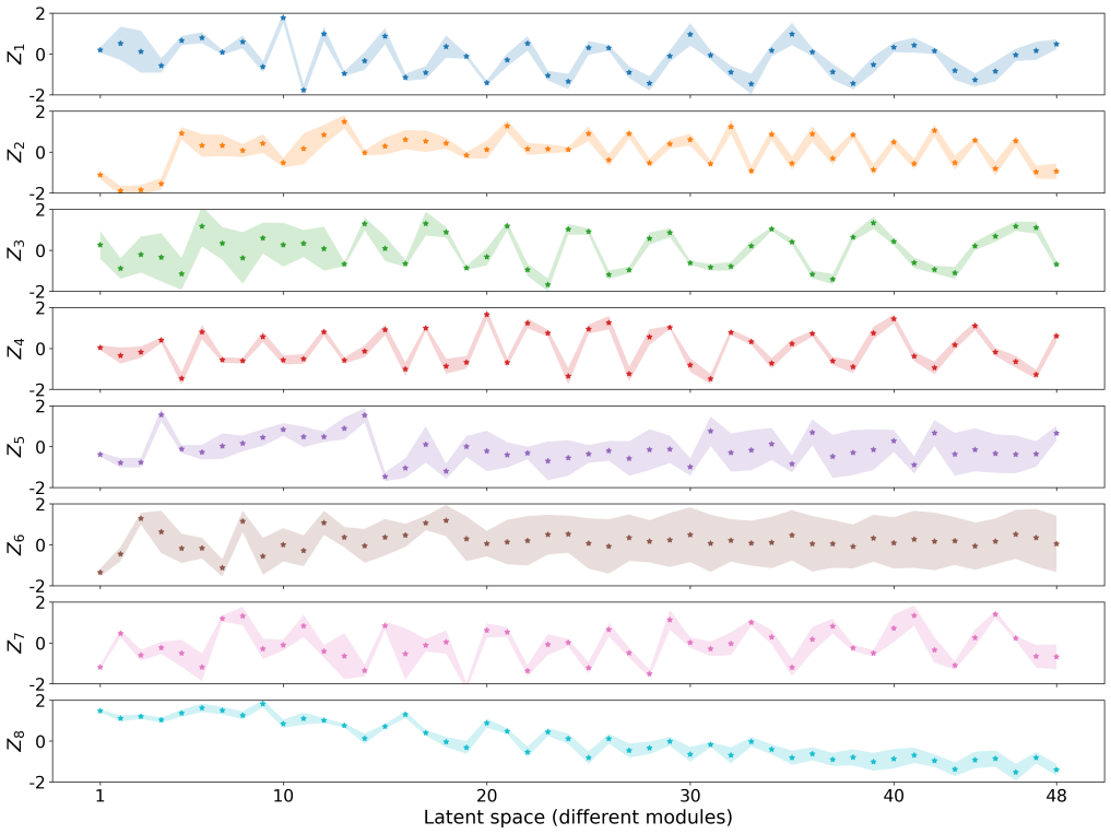
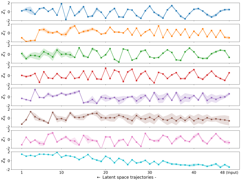
Another interesting observation from Fig. 5 is that the trajectories are primarily centered and symmetrical around the center of the latent space in all dimensions except $Z_{8}$. This implies that by moving linearly in the $Z_{8}$ direction ([-2,2]) while keeping the other dimensions fixed at the origin, we can generate phase space projections for modules from 48 to 1 without the need for conditional sampling in those regions of the latent space. By visualizing the $Z_{8}$ direction in Fig. 3(top plot, last image), we can further see the evidence of the aforementioned observation. This demonstrates that a well-structured latent space can effectively generate new samples with customized properties [69, 65]. Further investigations into this topic can be pursued as part of future research.

In this study, we focus exclusively on encoding aleatoric uncertainty with the CVAE and propagating it using the LSTM network. We assume that epistemic uncertainty is negligible in this context, which is possible with enough training data and sufficient model expressiveness. This assumption is essential for developing a novel approach to aleatoric uncertainty analysis through latent space. Future research will address both epistemic uncertainty and total uncertainty analysis.

3.3.2 Aleatoric uncertainty propagation

We also evaluate the robustness of the trained LSTM in predicting upstream states under uncertain downstream measurements. To achieve this, we propagate the aleatoric uncertainty captured in the latent space through the trained LSTM model. Since the CVAE has learned the aleatoric uncertainty of the phase space projections, any uncertain measurement (real observation) at a downstream module can be thought as a random point in the latent space corresponding to that module. This assumption is valid only if the uncertainty of the real observation is well captured by the CVAE, which was trained with the simulated phase space projections corresponding to randomly varied RF settings in a range. In our work, the simulator (HPSim) used to collect the dataset is calibrated every six months with the real accelerator (LANSCE). The drifts within those six months are slow enough to reasonably assume that the measurement will fall within the bounds of our training dataset.

We conditionally sample the latent space corresponding to module 48 multiple times (1000 times) to represent these uncertain measurements. Using these multiple instances as inputs, the trained LSTM predicts the 8D latent points for all upstream modules (47 to 1). Since the LSTM is a deterministic model with no built-in model uncertainty, it provides a single prediction for each upstream module based on the downstream measurements. To capture epistemic uncertainty, future work could incorporate techniques such as a Mixed Density Network (MDN) layer [70] or Monte Carlo dropout [71] into the LSTM framework. These approaches could enable the model to deliver both a mean and a standard deviation for all upstream modules based on a single downstream input.

We decode all the predicted latent points (from LSTM) to generate images using the trained CVAE decoder and then filter out the trajectories corresponding to false positive images. To achieve this, we use a pre-trained ResNet-50 classifier to determine if the generated image belongs to the true class (true module), similar to the method described in [18]. Through this unsupervised filtering analysis, we determined that nearly 50 percent (approximately 520 out of 1000) of the trajectories are identified as true trajectories. We calculated the mean and standard deviations for these true trajectories and present them in Fig. 7.

Figure 7: Latent space trajectories for all 8 dimensions with mean and standard deviation bounds. 1000 latent points are randomly sampled from the conditional latent space of module 48 and provided as input to the LSTM to predict the latent points for the upstream modules.

The motivation for performing filtering analysis stems from the fact that no generator can consistently produce realistic images every time it is sampled. As demonstrated in [18], the precision of the generated images across different modules ranges between 90-100% – even with high accuracy, it is still reasonably unlikely that 48 sampled points generate a realistic trajectory. The variability is due to the intermixing areas of latent points from different modules in lower dimensions, as shown in the 2D PCA plots in Fig. 3. So, we perform filtering to distinguish bad trajectories.

The bounds of the upstream predictions in Fig.7 fall within the bounds of the latent space shown in Fig.5. This is confirmed by Fig. 6(b), which shows that the aggregate standard deviation of the predictions of upstream latent points ($\sqrt{\sum{\sigma_{LSpred_{1:8}}^{2}}}$ shown by the red curve) is lower than that of the entire latent space ($\sum{\sigma_{LS_{1:8}}^{2}}$ shown by the orange curve in Fig. 6(a)). This indicates that the predictions from the trained LSTM do not violate the bounds of the latent space, demonstrating the robustness of the trained LSTM when handling uncertain measurements. Additionally, there is a expected similarity in the increasing trend observed across all four curves in Fig. 6.

We have performed uncertainty analysis in the latent space, whereas measurements and predictions exists in the high-dimensional image space. Thus, the trajectories in the latent space are projected back into the high-dimensional space using the trained decoder to obtain phase space projections in various modules. Pixel-wise mean and standard deviation for the generated projections of all true trajectories (Fig. 7) are shown in Fig. 8. It can be observed that the pixel-wise standard deviation varies for each projection. Also, the overall pixel-wise aggregate standard deviation can be compared across different modules. Fig. 6(b) (green curve) shows an increasing trend, similar to the corresponding aggregate standard deviation of the latent space trajectories (red curve).

(a) $x-y$ projection

(b) $E-\phi$ projection

(c) $x^{\prime}-y^{\prime}$ projection

Figure 8: Pixel-wise mean and standard deviation of phase space projections decoded from the latent space trajectories.

Notable, for better visualization, the images in Fig. 8 are plotted on a un-normalized logarithmic scale to compress the wider range of pixel intensities and enhance contrast in low-intensity areas. As a result, the standard deviation images appear brighter than they would on a normalized non-logarithmic scale, but the aforementioned observation still holds.

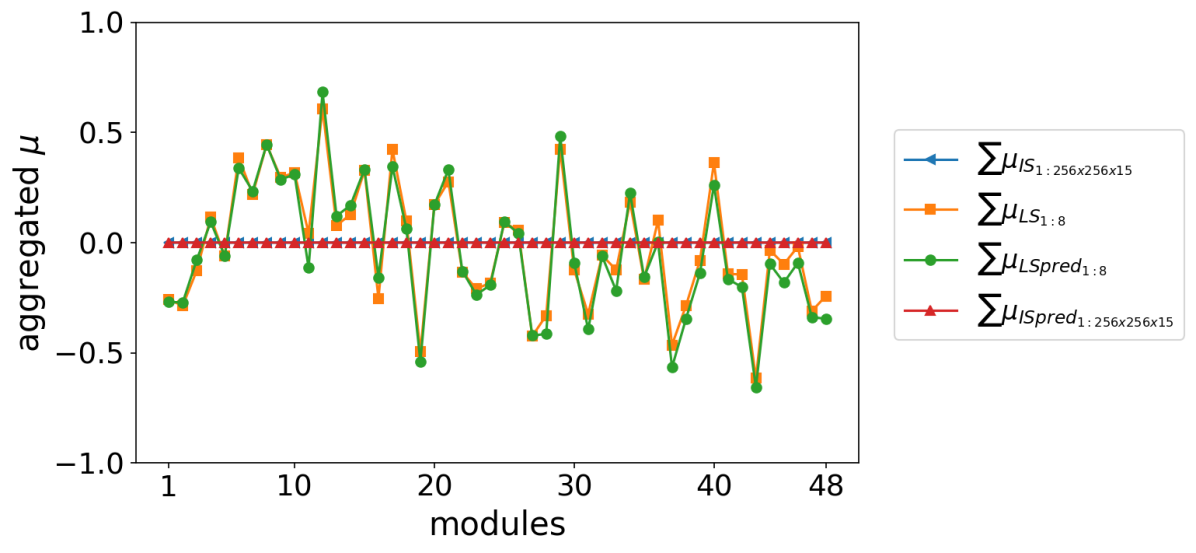
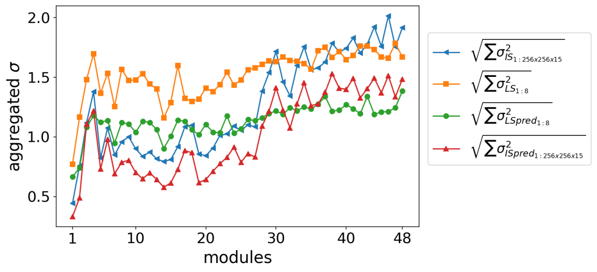
Four different aggregated standard deviation discussed in this section and shown with are Fig. 6 are complied together in a single plot, shown in Fig. A.1(b). In Fig. A.1(a), we plot four aggregated means (arithmetic mean of means). We see that the pixel-wise aggregated mean of images (dataset images with blue curve and decoded uncertain predictions with red curve) are zero across all the modules due to the normalization of the images between [0,1] and 0 zero regions of the image dominating non-zero regions. In their latent space version, we see that the aggregated mean matches closely, however, it is not zero. It fluctuates between [-0.5, 0.5] symmetrically with the zero line. Since, the latent points for different modules are clustered at different locations in the 8D space, aggregated mean provides the distance of the mean of latent points of a particular module on a real number line. Here, we want to emphasis that the aggregated mean in the latent space gives limited comparison power with the aggregated mean in the image space, contrary to what we discussed for aggregated standard deviation.

4 Conclusions

We have developed a reverse latent evolution model, a two-step self-supervised deep learning framework designed for the temporal inversion of spatiotemporal beam dynamics in particle accelerators. By utilizing an autoregressive CVAE-LSTM architecture, our framework predicts 15 unique projections of 6D phase space across all upstream accelerating sections based on downstream measurements. We enhance interpretability by visualizing the CVAE’s latent space using 2D PCA and t-SNE. The CVAE’s latent space effectively captures aleatoric uncertainty inherent in high-dimensional phase space projections. Uncertain latent points sampled conditionally from downstream modules are propagated to predict upstream latent points along with their associated uncertainty bounds. We demonstrate that the LSTM is robust against random perturbations of the input. High-dimensional phase space projections corresponding to these predictions are decoded from latent space trajectories, and presented with pixel-wise uncertainty bounds.

CRediT authorship contribution statement

Mahindra Rautela: Conceptualization, Methodology, Data curation, Formal analysis, Investigation, Writing - original draft, Writing—review and editing. Alan Williams: Data curation, Investigation, Writing—review and editing. Alexander Scheinker: Conceptualization, Methodology, Formal analysis, Investigation, Writing—review and editing, Funding acquisition, Supervision.

Declaration of competing interest

The authors declare that they have no known competing financial interests or personal relationships that could have appeared to influence the work reported in this paper.

Availability of codes and dataset

The data used in this article is available on Zenodo at
https://zenodo.org/records/10819001.

The code used in this article is available on GitHub at
https://github.com/mahindrautela/rLEM.

Appendix A

This appendix contains supplementary information in the form of additional results from Sec. 3.

Figure A.1: Comparison of (a) aggregated mean and (b) aggregate standard deviation of latent space (orange), Dataset image space (blue), LSTM based latent predictions (green), and decoded latent predictions (red).

Figure A.2: Comparison plot of two different random predictions ($A_{p}$/$A_{pred}$ and $B_{p}$/$B_{pred}$) from the trained rLEM at different upstream modules given two different module 48 as the input ($A_{t}$/$A_{true}$ and $B_{t}$/$B_{true}$): (a) $E-\phi$ projections (b) MSE vs module numbers.

(a) $x-y$ projection

(b) $E-\phi$ projection

(c) $x^{\prime}-y^{\prime}$ projection

Figure A.3: Predictions from the trained rLEM at different upstream modules given module 10 as the input.

(a) $x-y$ projection

(b) $E-\phi$ projection

(c) $x^{\prime}-y^{\prime}$ projection

Figure A.4: Predictions from the trained rLEM at different upstream modules given module 25 as the input.

References

- [1] R. Vinuesa, S. L. Brunton, Enhancing computational fluid dynamics with machine learning, Nature Computational Science 2 (6) (2022) 358–366.
- [2] E. Huerta, A. Khan, X. Huang, M. Tian, M. Levental, R. Chard, W. Wei, M. Heflin, D. S. Katz, V. Kindratenko, et al., Accelerated, scalable and reproducible ai-driven gravitational wave detection, Nature Astronomy 5 (10) (2021) 1062–1068.
- [3] A. Scheinker, F. Cropp, D. Filippetto, Adaptive autoencoder latent space tuning for more robust machine learning beyond the training set for six-dimensional phase space diagnostics of a time-varying ultrafast electron-diffraction compact accelerator, Physical Review E 107 (4) (2023) 045302.
- [4] A. Boehnlein, M. Diefenthaler, N. Sato, M. Schram, V. Ziegler, C. Fanelli, M. Hjorth-Jensen, T. Horn, M. P. Kuchera, D. Lee, et al., Colloquium: Machine learning in nuclear physics, Reviews of Modern Physics 94 (3) (2022) 031003.
- [5] A. Bormanis, C. A. Leon, A. Scheinker, Solving the orszag–tang vortex magnetohydrodynamics problem with physics-constrained convolutional neural networks, Physics of Plasmas 31 (1) (2024).
- [6] H. Morison, J. Singh, N. Al Kayed, A. Aadhi, M. Moridsadat, M. Tamura, A. N. Tait, B. J. Shastri, Nonlinear dynamics in neuromorphic photonic networks: Physical simulation in verilog-a, Physical Review Applied 21 (3) (2024) 034013.
- [7] T. N. Kipf, M. Welling, Semi-supervised classification with graph convolutional networks, arXiv preprint arXiv:1609.02907 (2016).
- [8] X. Shi, Z. Chen, H. Wang, D.-Y. Yeung, W.-K. Wong, W.-c. Woo, Convolutional lstm network: A machine learning approach for precipitation nowcasting, Advances in neural information processing systems 28 (2015).
- [9] M. Cheng, F. Fang, C. C. Pain, I. Navon, Data-driven modelling of nonlinear spatio-temporal fluid flows using a deep convolutional generative adversarial network, Computer Methods in Applied Mechanics and Engineering 365 (2020) 113000.
- [10] N. Wandel, M. Weinmann, R. Klein, Teaching the incompressible navier–stokes equations to fast neural surrogate models in three dimensions, Physics of Fluids 33 (4) (2021).
- [11] S. Wiewel, M. Becher, N. Thuerey, Latent space physics: Towards learning the temporal evolution of fluid flow, in: Computer graphics forum, Vol. 38, Wiley Online Library, 2019, pp. 71–82.
- [12] A. Scheinker, Adaptive machine learning for time-varying systems: low dimensional latent space tuning, Journal of Instrumentation 16 (10) (2021) P10008.
- [13] D. Montes de Oca Zapiain, J. A. Stewart, R. Dingreville, Accelerating phase-field-based microstructure evolution predictions via surrogate models trained by machine learning methods, npj Computational Materials 7 (1) (2021) 3.
- [14] T. Nakamura, K. Fukami, K. Hasegawa, Y. Nabae, K. Fukagata, Convolutional neural network and long short-term memory based reduced order surrogate for minimal turbulent channel flow, Physics of Fluids 33 (2) (2021).
- [15] R. Maulik, B. Lusch, P. Balaprakash, Reduced-order modeling of advection-dominated systems with recurrent neural networks and convolutional autoencoders, Physics of Fluids 33 (3) (2021).
- [16] P. R. Vlachas, G. Arampatzis, C. Uhler, P. Koumoutsakos, Multiscale simulations of complex systems by learning their effective dynamics, Nature Machine Intelligence 4 (4) (2022) 359–366.
- [17] A. Solera-Rico, C. Sanmiguel Vila, M. Gómez-López, Y. Wang, A. Almashjary, S. T. Dawson, R. Vinuesa, -variational autoencoders and transformers for reduced-order modelling of fluid flows, Nature Communications 15 (1) (2024) 1361.
- [18] M. Rautela, A. Williams, A. Scheinker, A conditional latent autoregressive recurrent model for generation and forecasting of beam dynamics in particle accelerators, Scientific Reports 14 (1) (2024) 18157.
- [19] M. Rautela, A. Scheinker, A. Williams, Towards latent space evolution of spatiotemporal dynamics of six-dimensional phase space of charged particle beams, Proc. IPAC’24 (2024) 906–909.
- [20] A. Scheinker, A. Edelen, D. Bohler, C. Emma, A. Lutman, Demonstration of model-independent control of the longitudinal phase space of electron beams in the linac-coherent light source with femtosecond resolution, Physical review letters 121 (4) (2018) 044801.
- [21] C. Emma, A. Edelen, M. Hogan, B. O’Shea, G. White, V. Yakimenko, Machine learning-based longitudinal phase space prediction of particle accelerators, Physical Review Accelerators and Beams 21 (11) (2018) 112802.
- [22] A. Ivanov, I. Agapov, Physics-based deep neural networks for beam dynamics in charged particle accelerators, Physical review accelerators and beams 23 (7) (2020) 074601.
- [23] C. Caliari, A. Oeftiger, O. Boine-Frankenheim, Identification of magnetic field errors in synchrotrons based on deep Lie map networks, Physical Review Accelerators and Beams 26 (6) (2023) 064601.
- [24] J. Zhu, Y. Chen, F. Brinker, W. Decking, S. Tomin, H. Schlarb, High-fidelity prediction of megapixel longitudinal phase-space images of electron beams using encoder-decoder neural networks, Physical Review Applied 16 (2) (2021) 024005.
- [25] D. Meier, L. V. Ramirez, J. Völker, J. Viefhaus, B. Sick, G. Hartmann, Optimizing a superconducting radio-frequency gun using deep reinforcement learning, Physical Review Accelerators and Beams 25 (10) (2022) 104604.
- [26] F. Mayet, M. Hachmann, K. Floettmann, F. Burkart, H. Dinter, W. Kuropka, T. Vinatier, R. Assmann, Predicting the transverse emittance of space charge dominated beams using the phase advance scan technique and a fully connected neural network, Physical Review Accelerators and Beams 25 (9) (2022) 094601.
- [27] F. Cropp, L. Moos, A. Scheinker, A. Gilardi, D. Wang, S. Paiagua, C. Serrano, P. Musumeci, D. Filippetto, Virtual-diagnostic-based time stamping for ultrafast electron diffraction, Physical Review Accelerators and Beams 26 (5) (2023) 052801.
- [28] O. Convery, L. Smith, Y. Gal, A. Hanuka, Uncertainty quantification for virtual diagnostic of particle accelerators, Physical Review Accelerators and Beams 24 (7) (2021) 074602.
- [29] A. Tran, Y. Hao, B. Mustapha, J. L. Martinez Marin, Predicting beam transmission using 2-dimensional phase space projections of hadron accelerators, Frontiers in Physics 10 (2022) 955555.
- [30] N. Breckwoldt, S.-K. Son, T. Mazza, A. Rörig, R. Boll, M. Meyer, A. C. LaForge, D. Mishra, N. Berrah, R. Santra, et al., Machine-learning calibration of intense X-ray free-electron-laser pulses using Bayesian optimization, Physical Review Research 5 (2) (2023) 023114.
- [31] C. Obermair, T. Cartier-Michaud, A. Apollonio, W. Millar, L. Felsberger, L. Fischl, H. S. Bovbjerg, D. Wollmann, W. Wuensch, N. Catalan-Lasheras, et al., Explainable machine learning for breakdown prediction in high gradient RF cavities, Physical Review Accelerators and Beams 25 (10) (2022) 104601.
- [32] K. Rajput, M. Schram, W. Blokland, Y. Alanazi, P. Ramuhalli, A. Zhukov, C. Peters, R. Vilalta, Robust errant beam prognostics with conditional modeling for particle accelerators, Machine Learning: Science and Technology 5 (1) (2024) 015044.
- [33] C. Tennant, A. Carpenter, T. Powers, A. S. Solopova, L. Vidyaratne, K. Iftekharuddin, Superconducting radio-frequency cavity fault classification using machine learning at jefferson laboratory, Physical Review Accelerators and Beams 23 (11) (2020) 114601.
- [34] Y. Li, W. Cheng, L. H. Yu, R. Rainer, Genetic algorithm enhanced by machine learning in dynamic aperture optimization, Physical Review Accelerators and Beams 21 (5) (2018) 054601.
- [35] S. Li, A. Adelmann, Time series forecasting methods and their applications to particle accelerators, Physical Review Accelerators and Beams 26 (2) (2023) 024801.
- [36] R. Bellotti, R. Boiger, A. Adelmann, Fast, efficient and flexible particle accelerator optimisation using densely connected and invertible neural networks, Information 12 (9) (2021) 351.
- [37] A. Scheinker, F. Cropp, S. Paiagua, D. Filippetto, An adaptive approach to machine learning for compact particle accelerators, Scientific reports 11 (1) (2021) 19187.
- [38] A. Wolski, M. A. Johnson, M. King, B. L. Militsyn, P. H. Williams, Transverse phase space tomography in an accelerator test facility using image compression and machine learning, Physical Review Accelerators and Beams 25 (12) (2022) 122803.
- [39] R. Roussel, A. Edelen, C. Mayes, D. Ratner, J. P. Gonzalez-Aguilera, S. Kim, E. Wisniewski, J. Power, Phase space reconstruction from accelerator beam measurements using neural networks and differentiable simulations, Physical Review Letters 130 (14) (2023) 145001.
- [40] R. C. Smith, Uncertainty quantification: theory, implementation, and applications, SIAM, 2013.
- [41] D. Zhang, L. Lu, L. Guo, G. E. Karniadakis, Quantifying total uncertainty in physics-informed neural networks for solving forward and inverse stochastic problems, Journal of Computational Physics 397 (2019) 108850.
- [42] A. Acharya, R. Russell, N. R. Ahmed, Learning to forecast aleatoric and epistemic uncertainties over long horizon trajectories, arXiv preprint arXiv:2302.08669 (2023).
- [43] A. Adelmann, On nonintrusive uncertainty quantification and surrogate model construction in particle accelerator modeling, SIAM/ASA Journal on Uncertainty Quantification 7 (2) (2019) 383–416.
- [44] A. A. Mishra, A. Edelen, A. Hanuka, C. Mayes, Uncertainty quantification for deep learning in particle accelerator applications, Physical Review Accelerators and Beams 24 (11) (2021) 114601.
- [45] W. Blokland, K. Rajput, M. Schram, T. Jeske, P. Ramuhalli, C. Peters, Y. Yucesan, A. Zhukov, Uncertainty aware anomaly detection to predict errant beam pulses in the oak ridge spallation neutron source accelerator, Physical Review Accelerators and Beams 25 (12) (2022) 122802.
- [46] M. Schram, K. Rajput, K. S. NS, P. Li, J. S. John, H. Sharma, Uncertainty aware machine-learning-based surrogate models for particle accelerators: Study at the fermilab booster accelerator complex, Physical Review Accelerators and Beams 26 (4) (2023) 044602.
- [47] C. Garcia-Cardona, A. Scheinker, Machine learning surrogate for charged particle beam dynamics with space charge based on a recurrent neural network with aleatoric uncertainty, Physical Review Accelerators and Beams 27 (2) (2024) 024601.
- [48] B. Uria, M.-A. Côté, K. Gregor, I. Murray, H. Larochelle, Neural autoregressive distribution estimation, The Journal of Machine Learning Research 17 (1) (2016) 7184–7220.
- [49] G. Papamakarios, T. Pavlakou, I. Murray, Masked autoregressive flow for density estimation, Advances in neural information processing systems 30 (2017).
- [50] G. Papamakarios, E. Nalisnick, D. J. Rezende, S. Mohamed, B. Lakshminarayanan, Normalizing flows for probabilistic modeling and inference, Journal of Machine Learning Research 22 (57) (2021) 1–64.
- [51] J. Ho, A. Jain, P. Abbeel, Denoising diffusion probabilistic models, Advances in neural information processing systems 33 (2020) 6840–6851.
- [52] A. Scheinker, D. Filippetto, F. Cropp, 6d phase space diagnostics based on adaptively tuned physics-informed generative convolutional neural networks, in: Journal of Physics: Conference Series, Vol. 2420, IOP Publishing, 2023, p. 012068.
- [53] B. Cathey, S. Cousineau, A. Aleksandrov, A. Zhukov, First six dimensional phase space measurement of an accelerator beam, Physical Review Letters 121 (6) (2018) 064804.
- [54] P. Tenenbaum, Lucretia: A matlab-based toolbox for the modelling and simulation of single-pass electron beam transport systems, in: Proceedings of the 2005 Particle Accelerator Conference, IEEE, 2005, pp. 4197–4199.
- [55] L. Young, J. Billen, The particle tracking code parmela, in: Proceedings of the Particle Accelerator Conference, Vol. 5, 2003, pp. 3521–3523.
- [56] X. Pang, L. Rybarcyk, Gpu accelerated online multi-particle beam dynamics simulator for ion linear particle accelerators, Computer Physics Communications 185 (3) (2014) 744–753.
- [57] D. Sagan, M. Berz, N. Cook, Y. Hao, G. Hoffstaetter, A. Huebl, C.-K. Huang, M. Langston, C. Mayes, C. Mitchell, et al., Simulations of future particle accelerators: issues and mitigations, Journal of Instrumentation 16 (10) (2021) T10002.
- [58] T. P. Wangler, RF Linear accelerators, John Wiley & Sons, 2008.
- [59] A. Scheinker, D. Scheinker, Extremum seeking for optimal control problems with unknown time-varying systems and unknown objective functions, International Journal of Adaptive Control and Signal Processing 35 (7) (2021) 1143–1161.
- [60] D. P. Kingma, M. Welling, Auto-encoding variational bayes, arXiv preprint arXiv:1312.6114 (2013).
- [61] M. Toneva, T. M. Mitchell, L. Wehbe, Combining computational controls with natural text reveals aspects of meaning composition, Nature computational science 2 (11) (2022) 745–757.
- [62] K. Sohn, H. Lee, X. Yan, Learning structured output representation using deep conditional generative models, Advances in neural information processing systems 28 (2015).
- [63] J. Yin, Z. Pei, M. C. Gao, Neural network-based order parameter for phase transitions and its applications in high-entropy alloys, Nature Computational Science 1 (10) (2021) 686–693.
- [64] H. Sak, A. Senior, F. Beaufays, Long short-term memory based recurrent neural network architectures for large vocabulary speech recognition, arXiv preprint arXiv:1402.1128 (2014).
- [65] M. Rautela, J. Senthilnath, A. Huber, S. Gopalakrishnan, Towards deep generation of guided wave representations for composite materials, IEEE Transactions on Artificial Intelligence (2022).
- [66] L. Van der Maaten, G. Hinton, Visualizing data using t-sne., Journal of machine learning research 9 (11) (2008).
- [67] M. Rautela, A. Maghareh, S. Dyke, S. Gopalakrishnan, Deep generative models for unsupervised delamination detection using guided waves, arXiv preprint arXiv:2308.05350 (2023).
- [68] Z. Huang, H. Lam, H. Zhang, Evaluating aleatoric uncertainty via conditional generative models, arXiv preprint arXiv:2206.04287 (2022).
- [69] L. Wang, Y.-C. Chan, F. Ahmed, Z. Liu, P. Zhu, W. Chen, Deep generative modeling for mechanistic-based learning and design of metamaterial systems, Computer Methods in Applied Mechanics and Engineering 372 (2020) 113377.
- [70] D. Ha, J. Schmidhuber, World models, arXiv preprint arXiv:1803.10122 (2018).
- [71] M. Rautela, S. Gopalakrishnan, J. Senthilnath, Bayesian optimized physics-informed neural network for estimating wave propagation velocities, arXiv preprint arXiv:2312.14064 (2023).