5cm(2cm, 2.2cm)
![]()
ONSEP: A Novel Online Neural-Symbolic Framework for Event Prediction Based on Large Language Model
Abstract
In the realm of event prediction, temporal knowledge graph forecasting (TKGF) stands as a pivotal technique. Previous approaches face the challenges of not utilizing experience during testing and relying on a single short-term history, which limits adaptation to evolving data. In this paper, we introduce the Online Neural-Symbolic Event Prediction (ONSEP) framework, which innovates by integrating dynamic causal rule mining (DCRM) and dual history augmented generation (DHAG). DCRM dynamically constructs causal rules from real-time data, allowing for swift adaptation to new causal relationships. In parallel, DHAG merges short-term and long-term historical contexts, leveraging a bi-branch approach to enrich event prediction. Our framework demonstrates notable performance enhancements across diverse datasets, with significant Hit@k (k=1,3,10) improvements, showcasing its ability to augment large language models (LLMs) for event prediction without necessitating extensive retraining. The ONSEP framework not only advances the field of TKGF but also underscores the potential of neural-symbolic approaches in adapting to dynamic data environments.
1 Introduction
Event prediction is a widely researched topic Zhao (2021); Benzin and Rinderle-Ma (2023) since accurate prediction of future events allows one to minimize losses associated with certain future events. To model large amounts of real-world event data that represent complex interactions between entities over time, the temporal knowledge graph (TKG) has been introduced Ding et al. (2023); Yuan et al. (2023). TKG is used to represent structural relationships among entities through timestamped quadruples , where and are entities, is a binary relation between them, and specifies the time when the event occurs. For example, the quadruple indicates that Angela Merkel visited China on July 4, 2014. In this task, temporal knowledge graph forecasting (TKGF) aims to predict future events of the graph by inferring missing entities in a quadruple for a future time. This involves generating predictions for either the object entity or the subject entity by utilizing historical data from previous snapshots, where represents the number of time steps or intervals into the future beyond the current time . Existing research studies have provided theoretical methodologies for time-sensitive applications such as recommendation systems Wang et al. (2022); Zhao et al. (2022), financial analysis Li (2023), and social crisis early warning systems Gastinger et al. (2023).
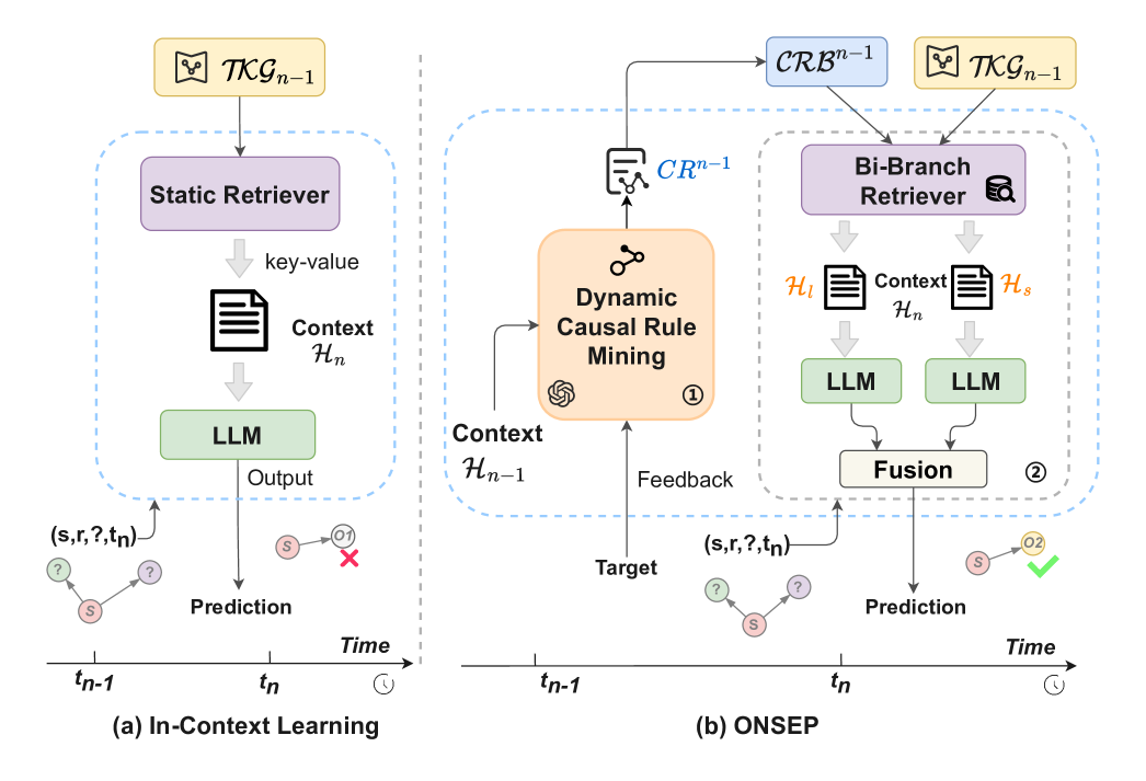
Traditional approaches Jin et al. (2020); Zhu et al. (2021); Li et al. (2021); Han et al. (2020); Sun et al. (2021); Li et al. (2022) involve converting event data into TKGs and combining graph neural networks (GNNs) and recurrent neural networks (RNNs) capture evolving entity relationships through embeddings. However, these methods must perform model training on specific datasets, which is resource-intensive. With the proven understanding and generative capabilities of large language models (LLMs), recent studies have explored methods on LLMs Tao et al. (2023); Lee et al. (2023); Shi et al. (2023b). The method proposed by Lee et al. (2023) offers a more adaptable method for TKGF with in-context learning (ICL) on LLMs, allowing LLMs to adapt to TKGF by using examples in the context, without fine-tuning.
Nevertheless, due to limitations in the length of history of LLM inputs, this approach may not fully capture long-term trends among events and cannot effectively leverage past insights, such as causal relationships between events. Imagine a TKG scenario that relates to everyday life. An example quadruple could be: ‘(, , , )’, indicating that Sarah consulted Dr. Smith on April 10, 2022. In this case, the ICL method may use static key values like ‘’ and ‘’ to extract historical events. However, this method may not account for Sarah’s tendency to begin consultations with phone calls months before meeting in person, This is evident in events such as ‘’ being a preceding cause, for example, ‘(, , )’. This long-standing pattern of initiating consultations with a call is a crucial piece of historical context that short-term data analysis could miss. Without considering these longer-term causal interactions, the LLM-based method may not make accurate future predictions. Besides, in datasets like ICEWS Boschee et al. (2015), the distribution of data containing entities and relations is dynamically changing. The emergence of new relations during test time poses challenges for traditional ICL methods, which rely on fixed keyword-key value matching and cannot adapt over time. This highlights the need for methods that can dynamically capture and apply updates in real-time, enhancing adaptability in event prediction.
To overcome these limitations, this paper proposes the Online Neural-Symbolic Event Prediction (ONSEP) framework. It enhances both accuracy and adaptability in event prediction by addressing inadequate long-term causal relationship capture and enabling real-time adaptability for self-improvement without fine-tuning. Figure 1 illustrates a comparison of the ONSEP and ICL approaches. By contrast, ONSEP mainly has two novel components: 1) Dynamic causal rule mining (DCRM): Utilizing LLMs’ external knowledge, DCRM semantically detects cause-effect links and dynamically constructs causal rules. This enables ONSEP to quickly adapt to new data and causal relationships, facilitating real-time updates and leveraging past experiences without extensive retraining. 2) Dual History Augmented Generation (DHAG): DHAG employs the long short-term bi-branch retriever (LSBBR) and a hybrid model inference (HMI) strategy to merge short-term and long-term historical contexts. The latter benefits from causal rules derived during the DCRM phase, enabling a broader event to be captured within the limits of historical input length. Inspired by the multi-branch fusion inference technology described in Shi et al. (2023a), the HMI strategy applies weighted fusion to balance the contributions from both dual historical contexts. These innovations address the limitations of context length constraints in LLMs and improve the retrieval of relevant historical events over extended periods.
ONSEP shows significant performance gains on various datasets using InternLM2-7B model, achieving Hit@1 improvements over ICL of 9.63%, 9.35%, and 16.28% at history length 100, and 8.14%, 8.64%, and 15.25% at 200, and achieved competitive performance of embedding-based models trained on specific datasets. To summarize, our main contributions include:
-
•
We introduce DCRM, an innovative real-time adaptive causal learning module for LLMs that automatically updates the rule base at the snapshot level during testing.
-
•
We develop the DHAG module, which uses LSBBR and HMI strategies, allowing LLMs to effectively use historical data from different time scales for causal analysis.
-
•
Our framework includes an adaptive RAG solution that improves historical event retrieval and achieves self-improvement.
-
•
We demonstrate ONSEP’s effectiveness across various models and datasets, showcasing its ability to enhance black-box LLM inference without the need for fine-tuning or manual annotations, thereby providing a robust and adaptable solution for diverse event prediction tasks.
2 Preliminaries
2.1 Temporal Knowledge Graph Forecasting
A temporal knowledge graph (TKG) is structured as a time-sequenced series of multi-relational directed graphs. The TKG up to time is represented as , where each represents a snapshot of the graph at time . Here, denotes the set of entities, the set of relations, and comprises timestamped facts as quadruples , with and . TKGF aims to predict future states of the graph by inferring missing entities in a quadruple for a future time. This involves generating predictions for either the object entity or the subject entity using historical data from previous snapshots .
2.2 ICL for Temporal Knowledge Graph Forecasting
ICL enables LLMs to adjust to new tasks through contextual examples, without the need for fine-tuning. Specifically, in TKGF, ICL harnesses the adaptability of LLMs for forecasting by leveraging historical data. For a query of future event , where is an entity and is a relation at timestamp , this method employs static keys, such as entity or the pair , to retrieve the historical event chain , a set of quadruples, from previous snapshots . Then the method constructs a prompt based on . The prediction is generated by leveraging the LLM’s probability distribution , employing ICL to generate forecasts without further training.
To effectively handle multi-word entity and relation names, a numeric mapping and assigns unique labels to entities and relations. For example, candidate entities like [South Africa, China, New England] are mapped to numerical values [0, 1, 2] to align the outputs from the LLM with these candidates. During in-context learning, LLMs perform a forward pass to produce logits for next-token predictions. These logits are then transformed into a probability distribution using the softmax function, representing the likelihood of each candidate being the target entity or relation.
2.3 Causal Rules in TKG
Causal rules111In this work, we use ”causal” to intuitively convey the role these rules play in identifying and retrieving events with potential causative relations during real-time analysis, differing from the strict definition in statistical causal inference. in TKG capture cause-and-effect links between events, denoted as , where and represent anonymized entities, and and are timestamps, with ensuring the correct temporal sequence from cause to effect.
Extending this, we define a causal rule base () as a set of tuples, each comprising a causal rule (CR) and its confidence score (conf). The for effect at timestamp is denoted as: , where indicates the cause relation, denotes the resulting relation influenced by , and is the confidence score for the -th causal rule at timestamp , a real number within . Here, represents the total number of causal rules considered in the rule base.
3 Method
The ONSEP framework (Figure 2) aims for event prediction via two key modules: (1) DCRM, which adaptively adjusts to changing data distributions during single-step prediction testing without requiring extensive training data, and (2) DHAG, which integrates patterns from short-term historical events with causality from long-term event developments. Detailed explanations are provided in the following sections.
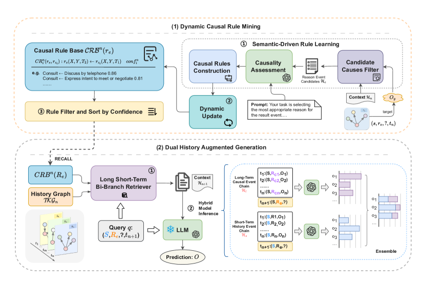
3.1 Dynamic Causal Rule Mining
The dynamic causal rule mining (DCRM) phase is crucial for identifying causal relationships within temporal knowledge graph. This phase utilizes a semantic-driven rule learning algorithm to discover causal rules. It is followed by a dynamic update module that updates the causal rule base (), which is closely followed by a mechanism for rule filtering and sorting by confidence.
3.1.1 Semantic-Driven Rule Learning
This module is designed for the reflective learning of causal rules, structured around three core steps: candidate causes filter, causality assessment, and causal rule construction. Initially, it retrieves historical context for all queries from and real-time feedback , which is the verified outcome for a query obtained when the system receives new data, to filter potential reason events. In the causality assessment phase, these candidates are then evaluated using a LLM to determine the most plausible cause event . Finally, the identified cause event, along with the query’s effect event forms the basis for constructing a causal rule . The algorithm of semantic-driven rule learning is outlined in Appendix A.
Candidate Event Filter
In the candidate event filtering phase, we utilize historical context and real-time feedback related to the query to filter potential causal events. Given a query at time , we define the context as a historical sequence of events associated with subject , expressed as . We select candidates based on the criterion that the object is the same as the target , thereby forming a set of candidate reason events , formalized as:
Here, represents a potential causal relation, is the filtered object that matches the target , and is the timestamp associated with the event. This methodology aims to pinpoint potential causative relations corresponding to within the event sequence that links the query’s subject to the target entity.
For each distinct causative event within the candidates of reason events, we first extract the set of quadruples from that contain , which we denote as :
We then compute the support number as the count of quadruples of this set: Subsequently, we calculate the coverage rate for each event using:
| (1) |
This coverage rate aids in assessing the confidence level of causal rules and supports the review and selection of causal event candidates by the LLM.
Causality Assessment
| LLM-based Causal Event Selection |
|---|
| Your task is selecting the most appropriate reason for the result event. The result event is { r_e }. |
| Below is a list of possible reasons: |
| { candidate causal events: [label]. [candidate] } |
| The most appropriate reason is: |
In this step, the causal evaluation utilizes the powerful semantic understanding capabilities of the LLM to assess the degree of causal association between a set of potentially causal events. This evaluation aims to select the causal rules that are most relevant to the current query and feedback goals. A pivotal aspect of our methodology involves the formulation of a structured prompt (Table 1), designed to direct the LLM towards discerning the most pertinent causal link between a given result event () and potential causes within the candidate reason events set . The selection mechanism utilizes LLM to obtain the logits for numerically mapped candidate reasons, as same as the way how to generate an output for each test query. These logits represent the preliminary evaluation of each candidate’s likelihood to be the true causal event. To convert these logits into normalized probabilities, we apply the softmax function, yielding the probability for each candidate reason , mapped to label using , reprented as , where are the logits produced by LLM, The probability of each candidate reason is then computed by:
| (2) |
Based on these probabilities, the top- candidates are selected. The confidence for each causal rule at timestamp is determined by combining the probability with the coverage score , can obtained as:
| (3) |
where is a tuning parameter that balances the contribution of the probability and the coverage score , integrating the causal assessment with historical occurrence insights.
Causal Rule Construction
Following the causality assessment step, a set of selected causal events () and their corresponding confidence scores at the current time step () are obtained. These causal rules are formalized in a structured format, with each rule at timestamp represented as , accompanied by a confidence value , can be obtained by
3.1.2 Dynamic Update
The dynamic update module for the causal rule base adds new rules directly and updates existing ones by adjusting their confidence levels. It assigns a confidence score to each causal rule , linking a pair of relations, and this score is dynamically updated at each time step . This score merges the previous confidence with the current confidence calculated at time , effectively updating the confidence for each pair of relations within the causal rule.
It uses a smoothing factor () to stabilize confidence adjustments, and a growth factor () to incrementally evaluate the reliability of the circular verification rules, but the historical confidence cannot exceed 1. The update formula of the existing rules is:
| (4) |
| (5) |
where is the updated confidence, the current evaluated confidence of , and the previous confidence, represent the grow function with the growth factor .
This approach ensures continuous optimization of the rule base, allowing for adaptability in light of distribution changes over time.
3.1.3 Rule Filter and Sort by Confidence
In the final module of the DCRM, rules falling below a predefined confidence threshold, denoted as , are filtered out to ensure the usability of the causal rule base. Subsequently, the remaining rules are sorted based on their confidence levels, allowing rules with higher confidence to take precedence in the subsequent reasoning phase.
3.2 Dual History Augmented Generation
DHAG, an innovative RAG variant, introduces a long short-term bi-branch retriever (LSTBBR) coupled with a hybrid model inference (HMI) strategy. DHAG synergizes short-term historical event patterns with long-term causal trajectories, ensuring a comprehensive historical context. Unlike previous methods that model long and short-term histories through data associations, DHAG provides a more robust handling of low-frequency events, unaffected by irrelevant noise in long histories.
3.2.1 Long Short-Term Bi-Branch Retriever
The long short-term bi-branch retriever (LSTBBR) within the DHAG framework incorporates a dual retrieval strategy to enhance the predictive model with a rich historical context, comprising both short-term and long-term historical events. For each prediction query , LSTBBR extracts two distinct historical contexts: representing the short-term history event chain and representing the long-term causal event chain. This dual approach ensures a comprehensive understanding of the immediate events as well as the underlying long-term causal influences. The short-term history event chain () focuses on capturing the most recent events that are temporally proximate to the prediction query, providing an immediate context that reflects the latest developments. To construct , the system retrieves events from , sorting them by timestamp and truncating to include only the most recent events. This truncated list of events forms , which is directly associated with the query’s subject , thereby providing a snapshot of the most immediate historical backdrop relevant to the query.
On the other hand, the long-term causal event chain () is designed to uncover the broader causal dynamics that have shaped the subject over a more extended period. This is achieved by initially retrieving cause rules from using a RECALL mechanism, which employs a key-value approach where the effect relation is used as the key to efficiently extract associated causal rules.
Subsequently, cause events are filtered to construct the long-term cause event chain from . The events in are determined by the criteria: where and , with . Similar to , is truncated to include only the most recent events since limited by the max length of model input.
3.2.2 Hybrid Model Inference
Before inference, a numerical label mapping technique preprocesses multi-word entities to prepare them for integration into the model, similar to the causality assessment in DCRM. The essence of the hybrid model inference (HMI) strategy involves merging the query with the short-term history event chain and the long-term causal event chain . This allows the LLM to produce distinct probabilities for each context, which are then combined using a weighted ensemble approach.
For the short-term context, the logits are obtained by , where symbolizes concatenation. The logits are then normalized using the softmax function to produce a probability distribution . Similarly, for the long-term context, the logits are derived by , and the corresponding probability distribution is obtained by applying the softmax function to , resulting in . The integration strategy involves a weighted ensemble of and , formulated as:
| (6) |
Here, is a tuning parameter that balances the contributions of short-term and long-term contexts. This unified distribution ranks candidate entities by their relevance to , leveraging the nuanced insights from both and . By doing so, the HMI strategy enhances the LLM’s accuracy in entity predictions, grounded in a comprehensive understanding of dual historical contexts.
4 Experiments
4.1 Experimental Settings
Datasets
Our experimental evaluation is carried out on a subset of the integrated crisis early warning system (ICEWS) dataset, which includes versions such as ICEWS14 García-Durán et al. (2018), ICEWS05-15 García-Durán et al. (2018), and ICEWS18 Jin et al. (2020). These datasets are composed of timestamped records of political events, making them highly suitable for conducting temporal analysis. They are widely recognized as benchmark datasets on TKGF. Each event is represented as a tuple, such as (Barack Obama, visit, Malaysia, 2014/02/19), capturing diverse political activities across various time periods.
Evaluation Metrics
To evaluate our method’s efficiency in ranking event candidates, we use link prediction metrics like Hit@k (where ). This measures the precision of our model in forecasting future events within the top predictions. Higher Hit@k values indicate more accurate rankings, which, in product recommendations, translate to better purchase predictions and greater economic benefits.
Baselines
We primarily compare ONSEP with the ICL method. Additionally, we have selected several traditional supervised models based on embedding methods for performance comparison, including RE-NET Jin et al. (2020), CyGNet Zhu et al. (2021), RE-GCN Li et al. (2021), xERTE Han et al. (2020), and TITer Sun et al. (2021) in TKG. We also compare our method with a variety of LLMs.
Further information about the datasets, evaluation metrics, LLMs used and implementation specifics can be found in the Appendix B.
| ICEWS14 | ICEWS05-15 | ICEWS18 | ||||||||
| Model | Train | Hit@1 | Hit@3 | Hit@10 | Hit@1 | Hit@3 | Hit@10 | Hit@1 | Hit@3 | Hit@10 |
| RE-NET | ✓ | 0.301 | 0.440 | 0.582 | 0.336 | 0.488 | 0.627 | 0.197 | 0.326 | 0.485 |
| CyGNet | ✓ | 0.274 | 0.426 | 0.579 | 0.294 | 0.461 | 0.616 | 0.172 | 0.310 | 0.469 |
| RE-GCN | ✓ | 0.316 | 0.472 | 0.617 | 0.373 | 0.539 | 0.685 | 0.224 | 0.368 | 0.527 |
| xERTE | ✓ | 0.327 | 0.457 | 0.573 | 0.378 | 0.523 | 0.639 | 0.210 | 0.335 | 0.465 |
| TITer | ✓ | 0.328 | 0.465 | 0.584 | 0.383 | 0.528 | 0.649 | 0.221 | 0.335 | 0.448 |
| InternLM2-7B-ICL (L=100) | ✗ | 0.301 | 0.432 | 0.560 | 0.353 | 0.507 | 0.647 | 0.172 | 0.289 | 0.434 |
| InternLM2-7B-ONSEP (L=100) | ✗ | 0.330 | 0.464 | 0.570 | 0.386 | 0.546 | 0.662 | 0.200 | 0.324 | 0.443 |
| Improve | 9.63% | 7.41% | 1.79% | 9.35% | 7.69% | 2.32% | 16.28% | 12.11% | 2.07% | |
| InternLM2-7B-ICL (L=200) | ✗ | 0.307 | 0.443 | 0.567 | 0.359 | 0.520 | 0.659 | 0.177 | 0.300 | 0.447 |
| InternLM2-7B-ONSEP (L=200) | ✗ | 0.332 | 0.465 | 0.577 | 0.390 | 0.551 | 0.668 | 0.204 | 0.333 | 0.453 |
| Improve | 8.14% | 4.97% | 1.76% | 8.64% | 5.96% | 1.37% | 15.25% | 11.00% | 1.34% | |
4.2 Performance Comparison
To evaluate whether ONSEP surpasses the previous best event prediction method based on LLMs, ICL, we conduct experiments with historical inputs of 100 and 200, using InternLM2-7B for all methods. As Table 2 shows, our method outperforms ICL across all three datasets. Specifically, with a history length of 100, ONSEP achieves Hit@1 improvements of 9.63%, 9.35%, and 16.28%, and with 200, the gains are 8.14%, 8.64%, and 15.25%. These results confirm ONSEP’s capability to exceed the performance of the previous ICL method. These results underscore ONSEP’s superior performance over ICL, particularly in Hit@1 accuracy, indicating a notable enhancement in precision.
While ONSEP trails behind some trained embedding models in Hit@10 due to the LLM’s reliance on ranking candidate entities from the input history rather than all entities, it achieves top performance in Hit@1 for the ICEWS14 and ICEWS05-15 datasets. Additionally, it shows closely competitive results in other metrics. This highlights ONSEP’s capability to significantly enhance accuracy. For a detailed exploration of ONSEP’s operational dynamics and its real-world applicability, see the ICEWS14 case study in Appendix C.
4.3 Inductive Setting and the Effectiveness of DCRM
| Method (InternLM2-7B) | Hit@1 | Hit@3 | Hit@10 | |
|---|---|---|---|---|
| (i) | ICL | 0.156 | 0.265 | 0.382 |
| (ii) | ONSEP | 0.186 | 0.305 | 0.424 |
| (iii) | ONSEP - inductive | 0.184 | 0.302 | 0.422 |
| (iv) | ONSEP w/o DCRM (ICL w/ DHAG) - inductive | 0.168 | 0.292 | 0.416 |
To assess the transferability of causal rules mined during test-time iterations, we conduct experiments where rules learned from ICEWS14 are applied to predictions on ICEWS18, with findings presented in Table 3. There are significant temporal spans and differences in data distribution between ICEWS14 and ICEWS18. For example, ICEWS18 includes entities such as Donald Trump, who served as the President of the United States from 2017 to 2021, which are not present in ICEWS14.
With only a 20.3% overlap (see Table 5) in entities between the two datasets, our inductive experimental setup demonstrates performance improvements. Comparing the ICL method without pre-loaded rules (i) to the approach using ICEWS14-derived rules (iv), we observe a significant performance boost in the latter, indicating that the DCRM-mined causal rules are generalizable across datasets with similar relational structures, thereby improving inference.
Further analysis on the DCRM module’s impact shows that incorporating DCRM (iii) versus not incorporating it (iv) leads to enhanced performance across all metrics, including a notable 9.52% increase in Hit@1. This underscores DCRM’s effectiveness in improving the accuracy and recall of inference.
Interestingly, real-time rule mining with DCRM without pre-loaded rules (ii) is slightly higher than that of the inductive setting (iii) (i.e., with pre-loading the rules learned from ), suggesting that relying on potentially outdated rules may hinder adaptation to new data. Due to the smoothing setup in dynamic updates, the old rule set may introduce some interference, hindering rapid adaptation to the new test set. This emphasizes the need for dynamic rule updates to ensure model relevance and effectiveness across varying datasets with dynamically changing distributions.
4.4 Effectiveness of DHAG
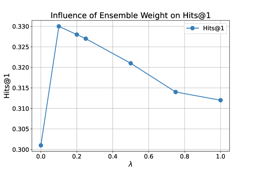
To assess the DHAG module’s impact, we explored how blending short-term and long-term history contexts affects performance on the ICEWS14 dataset, with similar findings observed on other datasets. We vary the Weighted Fusion Ratio from 0 to 1, as shown in Figure 3, with details in Appendix D.2.
Our findings indicate a clear pattern: a value of 0, which effectively uses only short-term history chain akin to the baseline ICL method, leads to lower performance. Conversely, a of 1, relying solely on long-term reasoning, also underperforms compared to a balanced approach. The optimal performance at a fusion ratio of 0.1 indicates that the model primarily utilizes short-term dynamic history for reasoning, while also incorporating long-term causal knowledge acquired during test time to improve its effectiveness.
4.5 Performance Comparison of Different Model Scale and Series
Our analysis reveals that model performance improves with increased parameter scale, with the 20B models outperforming the 7B models, aligning with the scaling law. However, the performance gain from increasing the model size from 7B to 20B is less pronounced and comes with higher computational costs. The ONSEP method enhances performance across different model scales and series, demonstrating its adaptability and effectiveness. Detailed comparisons across model series indicate that ONSEP’s improvements are consistent, with InternLM2-7b showing the most significant gains. Further in-depth analysis and discussions are provided in Appendix D.1.
4.6 Hyperparameter Sensitivity Analysis
Our hyperparameter sensitivity analysis highlights the critical role of selecting the right history length , rule selection thresholds , and fusion ratios for causal rule confidence scores. Finding the right balance between the length of historical input and computational efficiency is essential for optimal model performance. Similarly, precise calibration of rule selection thresholds and fusion ratios is vital for the effective application and updating of causal rules, taking into account factors such as the smoothing factor and growth factor . These parameters collectively influence the model’s ability to adapt and perform accurately over time. A more detailed discussion on these findings and their implications is provided in the Appendix E.
5 Related Work
5.1 Temporal Knowledge Graph Forecasting
In TKGF, traditional embedding-based methods Jin et al. (2020); Zhu et al. (2021); Li et al. (2021); Han et al. (2020); Sun et al. (2021); Li et al. (2022) learn representations of the quadruple, showing efficacy in supervised learning. Recent efforts explore LLMs for event prediction. For example, Xu et al. Xu et al. (2023) use a masking strategy to make the forecasting task similar to predicting missing words. LAMP Shi et al. (2023b) utilizes LLMs as a cause generator to reorder candidate outcomes, while ICL has been applied in TKGF Lee et al. (2023), transforming forecasting into a sequence generation task. Besides, GenTKG Liao et al. (2023) leverages few-shot parameter-efficient instruction tuning of LLMs using the training set to enhance inference capabilities. These approaches hold promise for improved generalization and contextual understanding. However, their effectiveness in dynamic real-world scenarios warrants further investigation.
On the other hand, rule-based approaches like Tlogic Liu et al. (2022) focus on interpretability and generalization by learning symbolic rules from TKGs. Despite their strengths, these methods struggle with large search spaces, can’t incorporate textual semantics of relations, and rely on static rule sets, limiting their adaptability.
5.2 Retrieve Augmented Generation
Retrieval-augmented generation (RAG) significantly enhances LLMs by integrating dynamic external knowledge retrieval Lewis et al. (2020), mitigating common challenges like hallucinations and slow information updates. Advancements like REPLUG Shi et al. (2023a) and AAR Yu et al. (2023) further enhance RAG. REPLUG refines retrieval models with supervised feedback from language models. AAR, on the other hand, is a versatile plug-in trained with a single source LLM but adaptable to various target LLMs. These adaptive mechanisms of RAG could be particularly beneficial in LLM-based TKGF, improving semantic alignment between queries and retrieved history context.
5.3 Self-Improving on LLMs
Researchers have recently proposed methods by using LLM’s inherent knowledge as an external database to let LLMs self-improve without annotated datasets and parameter updates. Frameworks like ExpNote Sun et al. (2023), HtT Zhu et al. (2023), and MoT Li and Qiu (2023) facilitate learning from experience, rule induction, and high-confidence thought generation. However, their application to tasks with temporal dimensions remains to be explored. Following this idea, we proposed an ONSEP framework to enable the model to induce rules in real-time during the testing process and then use them for future predictions.
6 Conclusion
In this paper, we introduce a novel online neural-symbolic framework, ONSEP, that integrates LLMs with TKGs to achieve adaptive and precise event forecasting in a dynamic online environment. To overcome the challenges of not utilizing experience during testing and relying on a single short-term history, which limits adaptation to new data, we propose a dynamic causal rule mining module and a dual history augmented generation module within the ONSEP framework. This design allows LLMs to access the most recent history to identify patterns, as well as causal relationships from a broader range of past events. Extensive experiments conducted on three benchmark datasets have proven the efficacy of ONSEP in TKGF, surpassing previous methods and demonstrating its broad applicability across diverse LLMs. Our framework shows great potential for future applications in financial forecasting, public sentiment monitoring, and recommendation systems.
Limitations
Our method requires multiple uses of large models, leading to increased inference time (see Appendix F) and higher computational costs compared to simpler models. The effectiveness of the model is influenced by the length of the input context; longer contexts are only useful for LLMs designed to handle them. The method also faces interpretability challenges due to unclear reasoning paths, which can be particularly evident in applications like campaign strategy analysis with the ICEWS dataset.
Additionally, the method’s potential to improve performance is limited for data that lacks a rich semantic understanding or detailed relationships needed to extract comprehensive causal rules. Since there is an upper limit on the length, the model inference uses indexing for the cue words and does not use the lexical setting, ignoring the effect of entity semantics on the results.
Ethics Statement
This paper presents a novel online neural-symbolic framework for event prediction, particularly tailored for dynamic real-world environments like TKGF. All experiments are conducted on publicly available datasets. Thus there is no data privacy concern. Meanwhile, this paper does not involve human annotations, and there are no related ethical concerns.
Acknowledgements
This work was supported in part by the National Key Research and Development Program of China under Grant 2022YFB3304602 and the National Nature Science Foundation of China under Grant 62003344.
References
- Bai et al. (2023) Jinze Bai, Shuai Bai, Yunfei Chu, Zeyu Cui, Kai Dang, Xiaodong Deng, Yang Fan, Wenbin Ge, Yu Han, Fei Huang, et al. 2023. Qwen technical report. ArXiv preprint, abs/2309.16609.
- Benzin and Rinderle-Ma (2023) Janik-Vasily Benzin and Stefanie Rinderle-Ma. 2023. A survey on event prediction methods from a systems perspective: Bringing together disparate research areas. arXiv preprint arXiv:2302.04018.
- Black et al. (2022) Sidney Black, Stella Biderman, Eric Hallahan, Quentin Gregory Anthony, Leo Gao, Laurence Golding, Horace He, Connor Leahy, Kyle McDonell, Jason Phang, et al. 2022. Gpt-neox-20b: An open-source autoregressive language model. In Challenges & Perspectives in Creating Large Language Models.
- Boschee et al. (2015) E. Boschee, J. Lautenschlager, S. O’Brien, S. Shellman, J. Starz, and M. Ward. 2015. ICEWS Coded Event Data.
- Ding et al. (2023) Zifeng Ding, Zongyue Li, Ruoxia Qi, Jingpei Wu, Bailan He, Yunpu Ma, Zhao Meng, Shuo Chen, Ruotong Liao, Zhen Han, et al. 2023. Forecasttkgquestions: A benchmark for temporal question answering and forecasting over temporal knowledge graphs. In International Semantic Web Conference, pages 541–560. Springer.
- García-Durán et al. (2018) Alberto García-Durán, Sebastijan Dumančić, and Mathias Niepert. 2018. Learning sequence encoders for temporal knowledge graph completion. In Proceedings of the 2018 Conference on Empirical Methods in Natural Language Processing, pages 4816–4821, Brussels, Belgium. Association for Computational Linguistics.
- Gastinger et al. (2023) Julia Gastinger, Nils Steinert, Sabine Gründer-Fahrer, and Michael Martin. 2023. Dynamic representations of global crises: Creation and analysis of a temporal knowledge graph for conflicts, trade and value networks.
- Han et al. (2020) Zhen Han, Peng Chen, Yunpu Ma, and Volker Tresp. 2020. xerte: Explainable reasoning on temporal knowledge graphs for forecasting future links. ArXiv preprint, abs/2012.15537.
- Jin et al. (2020) Woojeong Jin, Meng Qu, Xisen Jin, and Xiang Ren. 2020. Recurrent event network: Autoregressive structure inferenceover temporal knowledge graphs. In Proceedings of the 2020 Conference on Empirical Methods in Natural Language Processing (EMNLP), pages 6669–6683, Online. Association for Computational Linguistics.
- Lee et al. (2023) Dong-Ho Lee, Kian Ahrabian, Woojeong Jin, Fred Morstatter, and Jay Pujara. 2023. Temporal knowledge graph forecasting without knowledge using in-context learning. ArXiv preprint, abs/2305.10613.
- Lewis et al. (2020) Patrick S. H. Lewis, Ethan Perez, Aleksandra Piktus, Fabio Petroni, Vladimir Karpukhin, Naman Goyal, Heinrich Küttler, Mike Lewis, Wen-tau Yih, Tim Rocktäschel, Sebastian Riedel, and Douwe Kiela. 2020. Retrieval-augmented generation for knowledge-intensive NLP tasks. In Advances in Neural Information Processing Systems 33: Annual Conference on Neural Information Processing Systems 2020, NeurIPS 2020, December 6-12, 2020, virtual.
- Li (2023) Xiaohui Victor Li. 2023. Findkg: Dynamic knowledge graph with large language models for global finance. Available at SSRN 4608445.
- Li and Qiu (2023) Xiaonan Li and Xipeng Qiu. 2023. Mot: Memory-of-thought enables chatgpt to self-improve. In The 2023 Conference on Empirical Methods in Natural Language Processing.
- Li et al. (2022) Yujia Li, Shiliang Sun, and Jing Zhao. 2022. Tirgn: time-guided recurrent graph network with local-global historical patterns for temporal knowledge graph reasoning. In Proceedings of the Thirty-First International Joint Conference on Artificial Intelligence, IJCAI 2022, Vienna, Austria, 23-29 July 2022, pages 2152–2158. ijcai. org.
- Li et al. (2021) Zixuan Li, Xiaolong Jin, Wei Li, Saiping Guan, Jiafeng Guo, Huawei Shen, Yuanzhuo Wang, and Xueqi Cheng. 2021. Temporal knowledge graph reasoning based on evolutional representation learning. In Proceedings of the 44th international ACM SIGIR conference on research and development in information retrieval, pages 408–417.
- Liao et al. (2023) Ruotong Liao, Xu Jia, Yunpu Ma, and Volker Tresp. 2023. Gentkg: Generative forecasting on temporal knowledge graph. In Temporal Graph Learning Workshop@ NeurIPS 2023.
- Liu et al. (2022) Yushan Liu, Yunpu Ma, Marcel Hildebrandt, Mitchell Joblin, and Volker Tresp. 2022. Tlogic: Temporal logical rules for explainable link forecasting on temporal knowledge graphs. In Proceedings of the AAAI conference on artificial intelligence, volume 36, pages 4120–4127.
- Sennrich et al. (2016) Rico Sennrich, Barry Haddow, and Alexandra Birch. 2016. Neural machine translation of rare words with subword units. In 54th Annual Meeting of the Association for Computational Linguistics, pages 1715–1725. Association for Computational Linguistics (ACL).
- Shi et al. (2023a) Weijia Shi, Sewon Min, Michihiro Yasunaga, Minjoon Seo, Rich James, Mike Lewis, Luke Zettlemoyer, and Wen-tau Yih. 2023a. Replug: Retrieval-augmented black-box language models. ArXiv preprint, abs/2301.12652.
- Shi et al. (2023b) Xiaoming Shi, Siqiao Xue, Kangrui Wang, Fan Zhou, James Y Zhang, Jun Zhou, Chenhao Tan, and Hongyuan Mei. 2023b. Language models can improve event prediction by few-shot abductive reasoning. ArXiv preprint, abs/2305.16646.
- Sun et al. (2021) Haohai Sun, Jialun Zhong, Yunpu Ma, Zhen Han, and Kun He. 2021. TimeTraveler: Reinforcement learning for temporal knowledge graph forecasting. In Proceedings of the 2021 Conference on Empirical Methods in Natural Language Processing, pages 8306–8319, Online and Punta Cana, Dominican Republic. Association for Computational Linguistics.
- Sun et al. (2023) Wangtao Sun, Xuanqing Yu, Shizhu He, Jun Zhao, and Kang Liu. 2023. Expnote: Black-box large language models are better task solvers with experience notebook. In The 2023 Conference on Empirical Methods in Natural Language Processing.
- Tao et al. (2023) Zhengwei Tao, Zhi Jin, Xiaoying Bai, Haiyan Zhao, Yanlin Feng, Jia Li, and Wenpeng Hu. 2023. Eveval: A comprehensive evaluation of event semantics for large language models. arXiv preprint arXiv:2305.15268.
- Team (2023) InternLM Team. 2023. Internlm: A multilingual language model with progressively enhanced capabilities.
- Touvron et al. (2023) Hugo Touvron, Louis Martin, Kevin Stone, Peter Albert, Amjad Almahairi, Yasmine Babaei, Nikolay Bashlykov, Soumya Batra, Prajjwal Bhargava, Shruti Bhosale, et al. 2023. Llama 2: Open foundation and fine-tuned chat models. ArXiv preprint, abs/2307.09288.
- Wang et al. (2022) Xiaolin Wang, Guohao Sun, Xiu Fang, Jian Yang, and Shoujin Wang. 2022. Modeling spatio-temporal neighbourhood for personalized point-of-interest recommendation. In Proceedings of IJCAI.
- Xu et al. (2023) Wenjie Xu, Ben Liu, Miao Peng, Xu Jia, and Min Peng. 2023. Pre-trained language model with prompts for temporal knowledge graph completion. ArXiv preprint, abs/2305.07912.
- Yang et al. (2023) Aiyuan Yang, Bin Xiao, Bingning Wang, Borong Zhang, Ce Bian, Chao Yin, Chenxu Lv, Da Pan, Dian Wang, Dong Yan, et al. 2023. Baichuan 2: Open large-scale language models. ArXiv preprint, abs/2309.10305.
- Yu et al. (2023) Zichun Yu, Chenyan Xiong, Shi Yu, and Zhiyuan Liu. 2023. Augmentation-adapted retriever improves generalization of language models as generic plug-in. ArXiv preprint, abs/2305.17331.
- Yuan et al. (2023) Chenhan Yuan, Qianqian Xie, Jimin Huang, and Sophia Ananiadou. 2023. Back to the future: Towards explainable temporal reasoning with large language models. arXiv preprint arXiv:2310.01074.
- Zhao (2021) Liang Zhao. 2021. Event prediction in the big data era: A systematic survey. ACM Computing Surveys (CSUR), 54(5):1–37.
- Zhao et al. (2022) Yuyue Zhao, Xiang Wang, Jiawei Chen, Yashen Wang, Wei Tang, Xiangnan He, and Haiyong Xie. 2022. Time-aware path reasoning on knowledge graph for recommendation. ACM Transactions on Information Systems, 41(2):1–26.
- Zhu et al. (2021) Cunchao Zhu, Muhao Chen, Changjun Fan, Guangquan Cheng, and Yan Zhang. 2021. Learning from history: Modeling temporal knowledge graphs with sequential copy-generation networks. In Thirty-Fifth AAAI Conference on Artificial Intelligence, AAAI 2021, Thirty-Third Conference on Innovative Applications of Artificial Intelligence, IAAI 2021, The Eleventh Symposium on Educational Advances in Artificial Intelligence, EAAI 2021, Virtual Event, February 2-9, 2021, pages 4732–4740. AAAI Press.
- Zhu et al. (2023) Zhaocheng Zhu, Yuan Xue, Xinyun Chen, Denny Zhou, Jian Tang, Dale Schuurmans, and Hanjun Dai. 2023. Large language models can learn rules. ArXiv preprint, abs/2310.07064.
Appendix A Algorithm of Semantic-Driven Rule Learning
In this section we introduce the Semantic-Driven Rule Learning algorithm in DCRM. The pseudo code can be found at algorithm 1.
Appendix B Experimental Details
In the experiment, we used the ICEWS data sets, including ICEWS14, ICEWS05-15 and ICEWS18, we use the training and validation sets to build historical graphs, which then serve to test our model’s predictive accuracy. The specific parameters are shown in the table 4.
B.1 Datasets
| Dataset | # Ents | # Rels | Train | Valid | Test | Interval |
|---|---|---|---|---|---|---|
| ICEWS14 | 7,128 | 230 | 74,845 | 8,514 | 7,371 | 24 hours |
| ICEWS05-15 | 10,094 | 251 | 368,868 | 46,302 | 46,159 | 24 hours |
| ICEWS18 | 23,033 | 256 | 373,018 | 45,995 | 49,545 | 24 hours |
ICEWS14 and ICEWS18 have significant differences in data distribution. Specifically, the number of entities in ICEWS18 far exceeds that in ICEWS14. This can be clearly demonstrated in the dataset statistics:
| Dataset | Entities | Relations | Time Span |
|---|---|---|---|
| ICEWS14 | 7,128 | 230 | 2014 |
| ICEWS18 | 23,033 | 256 | 2018 |
| Overlap | 4,685 | 226 | - |
| Overlap (%) | 20.3% | 88.3% | - |
B.2 Evaluation Metrics
To assess ONSEP’s ability to rank candidates for event prediction without recalling all entities, we use link prediction metrics like Hit@k (where k=1, 3, 10). Hit@k is an evaluation metric that measures how often the model correctly places entities within the top k positions of the ranking list for a given query. Our evaluation specifically focuses on a time-aware setting, where we apply filtering to remove valid candidates not pertinent to the specific query.
B.3 Baselines
All large models used in the paper’s experiments are shown here, and the series and parameters are reported, as shown in Table 6.
B.4 Implementation Details
The experimental setup for the ICL method aligns with that of TKG-ICL Lee et al. (2023), except for a change in the model. The input provided to the model is based on indexing rather than lexical content. For the 20B model, due to computational resource constraints, we employed a 4-bit quantization approach for loading the model and performing inference. All experiments were conducted on GeForce RTX 3090 GPU with 24GB Memory.
Appendix C Case Study
This section delves into the ICEWS14 case study, demonstrating ONSEP’s innovative approach in event prediction. The aim is to showcase the method’s operational dynamics and its practical relevance.
C.1 Operational Setup and Input Scenarios
Initially, consider an input history length limit of 5 events. For the query scenario involving a hypothetical entity Thief engaged in Use unconventional violence, ONSEP’s task is to predict potential outcomes based on past events. The ICL method, serving as a comparative baseline, identifies only a short-term history sequence. In contrast, ONSEP extends the analysis both short-term and long-term historical data as Figure 4 shows.
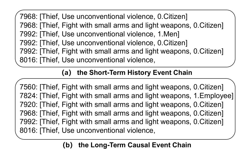
C.2 Causal Analysis and Predictive Accuracy
ONSEP employs learned causal rules to enhance prediction accuracy, for instance, inferring that Use unconventional violence may evolve from Fight with small arms and light weapons with a confidence score (: 0.76). This analysis is dynamically derived from both the LLM’s assessment and observed data frequencies.
When multiple rules apply, ONSEP retrieves relevant causative events from the historical graph for each rule and contextualizes them chronologically. This process leverages direct and precise causal relationships and enables ONSEP to integrate a broader range of historical insights, extending further back in time than baseline models. As the temporal dataset grows, ONSEP’s rule repository continuously evolves, improving the accuracy of historical context retrieval and updating the confidence levels of relational rules.
Appendix D Additional Experiment Results
D.1 Performance Comparison in Different Model Series
Model Scale
To analyze the impact of the model parameter scale on performance, we selected the 7B and 20B models from the InternLM2 series as the foundation models for ONSEP, with an input length of 100. As shown in Table 7, the 20B model performs better than the 7B model on the ICL method, consistent with our expectations and in line with the scaling law. The ONSEP method demonstrates significant improvements across both model scales, but the growth on the 20B model is relatively lower than on the 7B, and it is more time-consuming. The improvements in Hit@1 are 9.63% and 2.45% for the 7B and 20B models, respectively. This also proves that larger parameter LLMs have advantages in feature capturing, enabling better reasoning performance, but it’s important to consider the balance between performance gains and computational costs.
| Model | Hit@1 | Hit@3 | Hit@10 | Time | |
|---|---|---|---|---|---|
| InternLM2-7b-ICL | 0.301 | 0.432 | 0.560 | - | |
| InternLM2-7b-ONSEP | 0.330 | 0.464 | 0.570 | 2 h 32 min | |
| Improve | 9.63% | 7.41% | 1.79% | ||
| InternLM2-20b-ICL | 0.326 | 0.455 | 0.57 | - | |
| InternLM2-20b-ONSEP | 0.334 | 0.467 | 0.571 | 7h 10 min | |
| Improve | 2.45% | 2.64% | 0.18% |
Model Series
To compare the performance of different models under two scenarios and demonstrate ONSEP’s improvement over ICL, we use 7B models from the InternLM2, Qwen, LLaMA2, and Baichuan2 series. Figure 5 compares the performance of each model under ONSEP and ICL conditions. The comparison reveals that InternLM2-7b outperforms others with ICL and shows the most significant improvement with ONSEP, leading among models of similar size. While Qwen, LLaMA2, and Baichuan2 have similar performances with ICL, LLaMA2 and Qwen exhibit greater improvements with ONSEP than Baichuan2.
For the 20B models, we examine GPT-NeoX and InternLM2, as indicated in Table 8.
The performance differences may stem from variations in vocabulary, tokenization, training data, decoding strategies, and BPE encoding specifics Sennrich et al. (2016) among the different model series. InternLM2, with its innovative pre-training and optimization, excels in long-context tasks by capturing long-term dependencies. InternLM2’s superior performance may be due to a progressive training approach, starting with 4k tokens and extending to 32k tokens. ONSEP consistently enhances the performance across these models, showcasing the methodology’s generalizability. Additional metrics and detailed data are available in Appendix D.1.
| Model | Hit@1 | Hit@3 | Hit@10 |
|---|---|---|---|
| GPT-NeoX-20b-ICL | 0.314 | 0.446 | 0.560 |
| GPT-NeoX-20b-ONSEP | 0.320 | 0.454 | 0.563 |
| Improve | 1.91% | 1.79% | 0.54% |
| InternLM2-20b-ICL | 0.326 | 0.455 | 0.57 |
| InternLM2-20b-ONSEP | 0.334 | 0.467 | 0.571 |
| Improve | 2.45% | 2.64% | 0.18% |
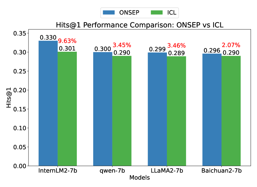
Table 9 shows the ICL methods for four different series of models of comparable size and the proposed ONSEP method. It is observed that InternLM2 performs the best in terms of various indicators and improvements. For Hit@1 and Hit@3, the performances of the other three models are similar, ranked in the order of Hit@1 as Qwen, Baichuan2, and Llama2. In terms of the improvement in Hit@10, the method achieved a 13.41% increase on Llama2. The pre-training data distribution and tokenization methods of these different open-source models vary, which impacts the performance.
| Model | Hit@1 | Hit@3 | Hit@10 |
|---|---|---|---|
| InternLM2-7b-ICL | 0.301 | 0.432 | 0.560 |
| InternLM2-7b-ONSEP | 0.330 | 0.464 | 0.570 |
| Improve | 9.63% | 7.41% | 1.79% |
| Qwen-7b-ICL | 0.290 | 0.421 | 0.530 |
| Qwen-7b-ONSEP | 0.300 | 0.440 | 0.560 |
| Improve | 3.4% | 4.51% | 5.66% |
| LLama2-7b-ICL | 0.289 | 0.412 | 0.440 |
| LLama2-7b-ONSEP | 0.299 | 0.438 | 0.499 |
| Improve | 3.5% | 6.31% | 13.41% |
| Baichuan2-7b-ICL | 0.290 | 0.416 | 0.530 |
| Baichuan2-7b-ONSEP | 0.296 | 0.437 | 0.552 |
| Improve | 2.06% | 5.05% | 4.15% |
D.2 Ensemble Weight in DHAG
Table 10 demonstrates the effect of adjusting the ensemble weight within the Dual History Augmented Generation (DHAG) of the ONSEP model on performance metrics Hit@1, Hit@3, and Hit@10. The data reveals that the optimal result for Hit@1 is achieved at , while the highest coverage rate for Hit@10 is observed at , indicating improvements in both metrics. Extreme values of (degenerating to the ICL method) lead to suboptimal outcomes, highlighting the dual context’s ability to enhance both accuracy and coverage, as well as the importance of balancing short-term and long-term historical contexts.
As increases, accuracy decreases, while the answer coverage remains constant, suggesting that DHAG enhances model performance by slightly increasing the probability of selecting the target (Hit@1).
| Ensemble Weight | Hit@1 | Hit@3 | Hit@10 |
|---|---|---|---|
| 0 | 0.301 | 0.432 | 0.560 |
| 0.1 | 0.330 | 0.464 | 0.570 |
| 0.2 | 0.328 | 0.462 | 0.571 |
| 0.25 | 0.327 | 0.462 | 0.572 |
| 0.5 | 0.321 | 0.460 | 0.573 |
| 0.75 | 0.314 | 0.456 | 0.572 |
| 1 | 0.312 | 0.445 | 0.552 |
Appendix E Hyperparameter Sensitivity Analysis
This section looks into how different hyperparameters affect our method. We use the ICEWS14 dataset and the InternLM2-7B model for this analysis, but we find similar patterns in other datasets too.
The set of tested hyperparameter ranges and best parameter values for ONSEP are displayed in Table 11. The best hyperparameter values are chosen based on the Hit@1.
| Hyperparameter | Set | Best |
|---|---|---|
| Ensemble Weight | {0, 0.1, 0.2, 0.25, 0.5, 0.75, 1} | 0.1 |
| History Length | {10, 30, 50, 100, 150, 200} | 200 |
| Select rules num | {0, 1, 3, 5, 10, 20} | 20 |
| Causality Ratio | {0, 0.1, 0.2, 0.25, 0.5, 0.75, 1} | 0.1 |
| Smooth Factor | {0, 0.25, 0.5, 0.75, 1} | 0.25 |
| Growth Factor | {0, 0.1, 0.15, 0.2, 0.25, 0.3, 0.5, 0.75, 1} | 0.2 |
E.1 History Length
We assess the impact of varying historical lengths on performance metrics (Hit@N) and the model’s inference time, as shown in Figure 6. Increasing historical length generally leads to better performance but also longer inference times. The most significant improvements occur up to a history length of 100; after that, the benefits level off, indicating an optimal balance between performance gains and computational efficiency is necessary.

Table 12 demonstrates the impact of different history lengths on model performance. As the history length increases, all performance metrics (Hit@1, Hit@3, and Hit@10) improve, but the growth saturates with longer . If computational resources are limited or fast inference is required, should be appropriately reduced to balance performance and efficiency.
| History Length | Hit@1 | Hit@3 | Hit@10 |
|---|---|---|---|
| 10 | 0.289 | 0.416 | 0.528 |
| 30 | 0.316 | 0.450 | 0.557 |
| 50 | 0.321 | 0.455 | 0.563 |
| 100 | 0.330 | 0.464 | 0.570 |
| 150 | 0.330 | 0.466 | 0.574 |
| 200 | 0.331 | 0.467 | 0.576 |
E.2 Maximum Number of Rules Selected
In the DCRM module, we experiment with changing the upper limit, K, of optimal rules selected after causality evaluation by the LLM. This parameter shows how selective we are in filtering causality semantics and influences the causal rule set size. As K increases, Hit@N performance improves, up to a certain point. Setting K to infinity (meaning no selection) causes a slight drop in performance from the optimum, suggesting that a larger rule set helps, but keeping high causality confidence is essential to minimize noise and avoid rule application disruption.
The results of selecting the maximum number of rules , as shown in 13, indicate that the model’s performance increases with the number of rules selected, reaching a saturation point. The last row suggests that not selecting rules after LLM evaluation results in slightly lower performance, highlighting the importance of optimal rule selection for achieving peak model effectiveness.
| Select rules num | Hit@1 | Hit@3 | Hit@10 |
|---|---|---|---|
| 0 | 0.318 | 0.454 | 0.561 |
| 1 | 0.327 | 0.461 | 0.569 |
| 3 | 0.328 | 0.462 | 0.570 |
| 5 | 0.329 | 0.462 | 0.570 |
| 10 | 0.330 | 0.464 | 0.570 |
| 20 | 0.329 | 0.462 | 0.570 |
E.3 Fusion Ratio of Causal Rule Confidence Scores
We experiment with various fusion ratios , mixing large model predicted probabilities and coverage from contextual frequencies to see their effect on performance. A balanced setting achieves optimal performance, highlighting the importance of both predicted probabilities and contextual coverage in determining causality confidence.
Regarding the fusion ratio of causal rule confidence scores , the table illustrates how adjusting affects model performance. The data in Table 14 show that the model performs best at Hit@1 with and reaches peak performance at Hit@3 with . This indicates that an appropriate value can balance the model’s prediction accuracy and coverage range. Too high or too low values may degrade performance on certain metrics.
| Causality Assessment Ratio | Hit@1 | Hit@3 | Hit@10 |
|---|---|---|---|
| 0 | 0.325 | 0.460 | 0.568 |
| 0.25 | 0.327 | 0.461 | 0.569 |
| 0.5 | 0.329 | 0.462 | 0.570 |
| 0.75 | 0.327 | 0.464 | 0.570 |
| 1 | 0.323 | 0.461 | 0.566 |
E.4 Causal Rule Confidence Update Function
In DCRM’s dynamic update process, adjusting causal rule confidence through factors like smoothing and growth is crucial for adapting to new data and trends. A balanced smoothing factor setting works well to incorporate both historical and new data, with larger values improving performance on the ICEWS dataset, suggesting stability is needed in dynamic data distributions. On the other hand, a careful setting of the growth factor improves performance. It shows the importance of slowly increasing focus on rules that have worked in the past without making their confidence scores too high too quickly.
smooth factor
The results for the smooth factor in the causal rule confidence update function ( 15) suggest that a moderate value balances historical and new information effectively. With a smooth factor of 0, the confidence scores are updated solely based on new samples, while a factor of 1 retains the initial confidence assessments. A slightly higher may be preferable for stable rule adaptation in dynamic data scenarios, whereas a lower value could be suitable if there are significant intervals between samples.
| Smooth Factor | Hit@1 | Hit@3 | Hit@10 |
|---|---|---|---|
| 0 | 0.325 | 0.462 | 0.570 |
| 0.25 | 0.330 | 0.464 | 0.570 |
| 0.5 | 0.327 | 0.463 | 0.570 |
| 0.75 | 0.327 | 0.462 | 0.571 |
| 1 | 0.324 | 0.461 | 0.566 |
growth factor
Table 16 shows that appropriately setting the growth factor can optimize model performance without being excessively high. A cautious, lower growth factor can incrementally increase attention to historically effective rules, enhancing their confidence scores. Conversely, too high a may introduce more noise, adversely affecting performance.
| Growth Factor | Hit@1 | Hit@3 | Hit@10 |
|---|---|---|---|
| 0 | 0.328 | 0.465 | 0.571 |
| 0.1 | 0.328 | 0.464 | 0.570 |
| 0.15 | 0.328 | 0.464 | 0.571 |
| 0.2 | 0.330 | 0.464 | 0.570 |
| 0.25 | 0.325 | 0.461 | 0.568 |
| 0.3 | 0.325 | 0.461 | 0.568 |
| 0.5 | 0.324 | 0.458 | 0.565 |
| 0.75 | 0.320 | 0.457 | 0.567 |
| 1 | 0.323 | 0.457 | 0.566 |
Appendix F Inference Time
Our tests on an RTX 3090 showed that ONSEP’s inference time (see Table 17) is about twice that of ICL due to multiple LLM calls, but it’s still suitable for scenarios like the ICEWS dataset where immediate real-time responses aren’t crucial.
| Model | ICEWS14 | ICEWS05-15 | ICEWS18 |
|---|---|---|---|
| InternLM2-7B-ICL (L=100) | 4.16 it/s | 3.14 it/s | 3.37 it/s |
| InternLM2-7B-ONSEP (L=100) | 1.94 it/s | 1.47 it/s | 1.66 it/s |