Differentiating Policies for Non-Myopic Bayesian Optimization
Abstract
Bayesian optimization (BO) methods choose sample points by optimizing an acquisition function derived from a statistical model of the objective. These acquisition functions are chosen to balance sampling regions with predicted good objective values against exploring regions where the objective is uncertain. Standard acquisition functions are myopic, considering only the impact of the next sample, but non-myopic acquisition functions may be more effective. In principle, one could model the sampling by a Markov decision process, and optimally choose the next sample by maximizing an expected reward computed by dynamic programming; however, this is infeasibly expensive. More practical approaches, such as rollout, consider a parametric family of sampling policies. In this paper, we show how to efficiently estimate rollout acquisition functions and their gradients, enabling stochastic gradient-based optimization of sampling policies.
1 Introduction
Bayesian optimization (BO) algorithms are sample-efficient methods for global optimization of expensive continuous “black-box” functions for which we do not have derivative information. BO builds a statistical model of the objective based on samples, and chooses new sample locations by optimizing an acquisition function that reflects the value of candidate locations. Most BO methods use myopic acquisition functions that only consider the impact of the next sample. Non-myopic strategies [33] may produce high-quality solutions with fewer evaluations than myopic strategies. One can define an “optimal” non-myopic acquisition function in terms of the expected reward for a Markov decision process. But because of the curse of dimensionality, an exact dynamic programming approach to compute such a function is computationally intractable in almost any problem of interest. Approximate methods such as rollout are more practical, but remain expensive.
This paper aims to make non-myopic BO more practical. In particular, our main contributions are:
-
•
We compute rollout acquisition functions via quasi-Monte Carlo integration and use variance reduction techniques to decrease the estimation error.
-
•
We introduce a trajectory-based formulation for deriving non-myopic acquisition functions using myopic functions—or any heuristic—as base heuristics.
-
•
We show how to differentiate rollout acquisition functions given a differentiable base policy.
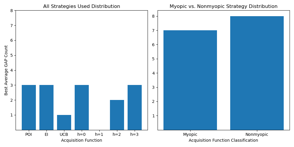
We show on a suite of test problems that we tend to do better than myopic policies when considered the best decrease in objective function from the first iteration to the last.
The subsequent sections of this paper discuss background and related work, including Gaussian Process Regression, Myopic Bayesian Optimization, Non-Myopic Bayesian Optimization, and Rollout Acquisition Functions (Sec. 2). Sec. 3 covers our models and methods, detailing our model and variance reduction techniques. We then explore our experimental results and their implications in Sec. 4. Limitations are discussed in Sec.5. The paper concludes with our final thoughts in Sec. 6.
2 Background and related work
Non-myopic Bayesian optimization has received a lot of attention over the past few years [5, 25, 19, 17, 16, 6, 2, 3, 33]. Much of this work involves rollout methods, in which one considers the expected best value seen over steps of a standard (myopic) BO iteration starting from a sample point under consideration. Rollout acquisition functions represent state-of-the-art in BO and are integrals over dimensions, where the integrand itself is evaluated through inner optimizations, resulting in an expensive integral that is typically evaluated by Monte Carlo methods. The rollout acquisition function is then maximized to determine the next BO evaluation, further increasing the cost. This large computational overhead has been observed by Osborn et al. [25], who are only able to compute rollout acquisition for horizon 2, dimension 1. Lam et al. [17], who use Gauss-Hermite quadrature in horizons up to five, saw runtimes on the order of hours for small, synthetic functions [3].
Recent work focuses on making rollout more practical. Wu and Frazier [3] consider horizon 2, using a combination of Gauss-Hermite quadrature [20] and Monte Carlo (MC) integration to quickly calculate the acquisition function and its gradient. Non-myopic active learning also uses rollout [4, 9, 10, 15] and recent work develops a fast implementation by truncating the horizon and selecting a batch of points to collect future rewards [9, 10].
2.1 Gaussian process regression
A Gaussian process (GP) is a collection of random variables, any finite number of which have a joint Gaussian distribution. Gaussian processes can be used to describe a distribution over functions. We place a GP prior on , denoted by , where and are the mean and covariance function, respectively. Here, is a kernel that correlates points in our sample space and it typically contains hyperparameters—like a lengthscale factor—that are learned to improve the quality of the approximation [28].
After observing at data points , the posterior distribution on is a GP. We assume the observations are where the are independent variables distributed as . Given , we define the following for convenience of representation:
The resulting posterior distribution for function values at a location x is the normal distribution :
| (1) | ||||
| (2) |
where is the identity matrix. GPs allow us to perform inference while quantifying our uncertainty. They also provide us with a mechanism for sampling possible belief states.
2.2 Myopic Bayesian optimization
Consider the problem of seeking a global minimum of a continuous objective over a compact set . If is expensive to evaluate, then finding a minimum should be sample-efficient. Myopic Bayesian Optimization (MBO) typically uses a GP to model from the data . The next evaluation location is determined by maximizing an acquisition function where the next sample is made based on a short-term view, looking only one step ahead:
In the myopic setting, our sequential decision-making problem makes choices that depend on all past observations, optimizing for some immediate reward. However, we usually have more than one step in our budget, so myopic acquisition functions are leaving something behind.
2.3 Non-myopic Bayesian optimization
Non-myopic BO frames the exploration-exploitation problem as a balance of immediate and future rewards. Lam et al. [17] formulate non-myopic BO as a finite horizon dynamic program; the equivalent Markov decision process follows.
The notation used is standard (see Puterman [26]): an MDP is a collection , where and is the set of decision epochs, finite for our problem. The state space, , encapsulates the information needed to model the system from time , and is the action space. Given a state and an action , is the probability the next state will be . is the reward received for choosing action in state and transitioning to .
A decision rule maps states to actions at time . A policy is a series of decision rules , one at each decision epoch. Given a policy , a starting state , and horizon , we can define the expected total reward as:
Our objective is to find the optimal policy that maximizes the expected total reward, i.e., , where is the space of all admissible policies.
If we can sample from the transition probability , we can estimate the expected total reward of any base policy — the decisions made using the base acquisition function — with MC integration [32]:
Given a GP prior over data with mean and covariance matrix , we model steps of BO as an MDP. This MDP’s state space is all possible data sets reachable from starting-state with steps of BO. Its action space is ; actions correspond to sampling a point in . Its transition probability and reward function are defined as follows. Given an action , the transition probability from to , where is:
Thus, the transition probability from to is the probability of sampling from the posterior at . We define a reward according to expected improvement (EI) [12]. Let be the minimum observed value in the observed set , i.e., . Then our reward is expressed as follows:
EI can be defined as the optimal policy for horizon one, obtained by maximizing the immediate reward:
where the starting state is —our initial samples. We define the non-myopic policy as the optimal solution to an -horizon MDP. The expected total reward of this MDP is:
The integrand is a telescoping sum, resulting in the equivalent expression on the rightmost side of the equation. When , the optimal policy is difficult to compute.
2.4 Rollout acquisition functions
Finding an optimal policy for the -horizon MDP is hard, partly because of the expense of representing and optimizing over policy functions. One approach to faster approximate solutions to the MDP is to replace the infinite-dimensional space of policy functions with a family of trial policies described by a modest number of parameters. An example of this approach is rollout policies [1], which yield promising results for the -step horizon MDP [3]. For a given state , we say that a base policy is a sequence of rules that determines the actions to be taken in various states of the system.
We denote our base policy for the -horizon MDP as . We let denote the initial state of our MDP and for to denote the random variable that is the state at each decision epoch. Each individual decision rule for consists of maximizing the base acquisition function given the current state , i.e.
Using this policy, we define the non-myopic acquisition function as the rollout of to horizon , i.e. the expected reward of starting with action :
where is the noisy observed value of at . Thus, as is the case with any acquisition function, the next BO evaluation is:
Rollout is tractable and conceptually straightforward, however, it is still computationally demanding. To rollout once, we must do steps of BO with . Many of the aforementioned rollouts must then be averaged to reasonably estimate , which is an -dimensional integral. Estimation can be done either through explicit quadrature or MC integration, and is the primary computational bottleneck of rollout.
3 Models and methods
3.1 Model
We build our intuition behind our approach from a top-down perspective. We have seen that non-myopic Bayesian optimization is promising, though tends to be computationally intractable. To circumvent this problem, we formulate a sub-optimal approximation to solve the intractable dynamic program; namely, a rollout acquisition function. Though relatively more tractable, rollout acquisition functions can be computationally burdensome. We are interested in solving where
| (3) |
and are sample trajectories. Sample trajectories consist of picking a starting point and asking “what would happen if I used my base policy from this point forward?” Since these trajectories don’t represent what did happen, rather what might, we call each realization a fantasized sample. Unfortunately, derivative-free optimization in high-dimensional spaces is expensive, so we would like estimates of . In particular, differentiating with respect to yields the following:
| (4) |
which requires some notion of differentiating sample trajectories. Thus, our problem can be expressed as two interrelated optimizations:
-
1.
An inner optimization for determining sample trajectories
-
2.
An outer optimization for determining our next query location
In what follows, we define how to compute and differentiate sample trajectories and how to differentiate the rollout acquisition function. We introduce the following notation to distinguish between two GP sequences that must be maintained. Suppose we have function values and gradients denoted as follows: . We define two GP sequences as:
The model, fundamentally, relies on the distinction amongst known sample locations , deterministic start location , and the stochastic fantasized sample locations . We denote a full trajectory including fantasized steps by:
Moreover, we collect the known samples into . The distinction between negative, null, and positive superscripts serves a useful purpose. Negative superscripts can be thought of as the past; potentially noisy observations that are fixed and immutable. The null superscripts denotes our freedom of choice; we are not bound to start at a specific location. Positive superscripts can be thought of as our ability to see into the future: things we anticipate on observing given our current beliefs.
Our problem is how to choose to maximize our expected reward over some finite horizon . We focus on developing an -step expected improvement (EI) rollout policy that involves choosing by using Stochastic Gradient Ascent (SGA) to optimize our rollout acquisition function.
An -step EI rollout policy involves choosing based on the anticipated behavior of the EI () algorithm starting from and proceeding for steps. That is, we consider the iteration
| (5) |
where the trajectory relations are
Trajectories are fundamentally random variables; their behavior is determined by the rollout horizon , start location x, base policy , and initial observation —denoted as . We denote sample draws as follows:
| (6) |

Computing this sample path, however, requires we solve the iteration defined above. We also use the notation to denote the -th element of the -th 3-tuple associated with the -th sample. Now that we have some provisional notation, we define how to evaluate as follows:
| (7) |
If we let , we can rewrite the minimum of the sample trajectory as follows:
| (8) |
Now, we are able to differentiate trajectories given by the following
| (9) |
which requires us to compute where . Hence, we have
| (10) |
Since the best function value found is a function of the best location , which is also a function of , we have
| (11) |
This captures how the best value found thus far changes as we vary the -th dimension of which is equivalently expressed as
| (12) |
From the trajectory relations defined above, we are able to derive the following relationship via the Implicit Function Theorem about :
We are able to compute the Jacobian matrix as
| (13) |
defining all of the computations necessary to solve the inner and outer optimization problem.
3.2 Methods
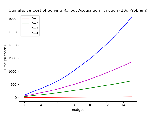
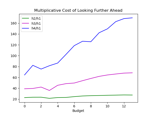
Significant computational challenges arise when computing the rollout acquisition function (RAF). Namely, rolling out the base acquisition function for steps consists of updating and maintaining a fantasized GP which is averaged across some monte-carlo simulations. Naive updates of the covariance and Cholesky matrix for each fantasized GP unnecessarily repeats computations. Another cost incurred when evaluating the rollout acquisition function (RAF) is that the -step iteration is solving an optimization problem at each step. Finally, in order to differentiate the RAF, we need to differentiate trajectories, requiring us to estimate a sequence of Jacobian matrices. In what follows, we address the following techniques to enable efficient computation and optimization of the RAF: smart linear algebra, quasi-monte carlo, common random numbers and control variates.
Differentiation of the base acquisition function Evaluating the rollout acquisition function necessitates the optimization of the base acquisiton function iteratively, for a total of times. To expedite this step, our approach uses the gradient and Hessian of the base policy. This enables us to use second-order optimization algorithms that significantly speeds up the optimization process.
Smart linear algebra. Maintaining GPs with an -step base policy for some evaluation of at location is expensive. The value of determines how many inner optimization problems we solve and we call the -step lookahead acquisition function. Computing a covariance matrix and it’s inverse is and , respectively. Doing this for our -step policy produces something on the order of for the covariance updates and for the matrix inversion updates. To circumvent this inefficiency, we preallocate matrices for both the covariance and Cholesky factorizations. This preallocation is dynamically updated using Schur’s complement. This approach yields a substantial reduction in computational load by making updates something on the order of a polynomial of a lower integer degree, thereby streamlining the inner optimization process.
3.2.1 Variance reduction techniques
Variance reduction is a set of methods that improve convergence by decreasing the variance of some estimator. Useful variance reduction methods can reduce the sample variance by several orders of magnitude [24]. We use a combination of quasi-Monte Carlo, common random numbers, and control variates, which significantly reduces the number of MC samples needed, while smoothing out estimates of the underlying stochastic objective.
Quasi-monte carlo. (QMC) Monte Carlo methods use independent, uniformly distributed random numbers on the -dimensional unit cube as the source of points to integrate at. The distribution we integrate over is Normal, for which a low-discrepancy sequence is known to exist. We generate low-discrepancy Sobolev sequences in the -dimensional uniform distribution and map them to the standard multivariate Gaussian via the Box-Muller transform [31]. This produces a low-discrepancy sequence for , allowing us to apply QMC by replacing the standard multivariate Gaussian samples with our low-discrepancy sequence.
Common random numbers (CRN). In many stochastic processes, different iterations or simulations use separate sets of random numbers to generate outcomes. While this approach is robust in ensuring the independence of each trial, it can also introduce a high degree of variability or noise into the results. This is where Common Random Numbers come into play. The CRN techniques involves using the same set of random numbers across different iterations. CRN does not decrease the pointwise variance of an estimate, but rather decreases the covariance between two neighboring estimates, which smooths out the function.
Control variates. A control variate is a variable that is highly correlated with the function of interest and has a known expected value. The key is to find a variable whose behavior is similar to that of the function being estimated. Since corresponds to an -step EI acquisition, we use the -step EI acquisition as our control variate. That is, we can estimate where . Given this construction, the variance of our estimator is given as follows:
The variance of our estimator is quadratic in and is minimized for . However, since is unknown, we estimate from the Monte Carlo simulations.
Overall, by combining smart linear algebra, quasi-Monte Carlo integration, common random numbers, and control variates, we show that computing and differentiating rollout acquisition functions is tractable.
4 Experiments and discussion
Throughout our experiments we use a GP with the Matérn 5/2 ARD kernel [30] and learn its hyperparameters via maximum likelihood estimation [27]. When rolling out acquisition functions, we maximize them using the Adam-variant of Stochastic Gradient Ascent (SGA) with expected improvement used as the base policy. We use the proposed default values for Adam of 0.9 for , for , and for [14]. We use the evidence-based criterion developed in [22] as our convergence criteria. We use random restarts for solving the inner optimization with a maximum of iterations for SGA and select the best point found. All synthetic functions are found in the supplementary.
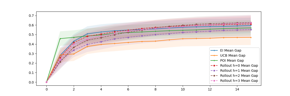
Given a fixed evaluation budget, we evaluate the performance of an algorithm in terms of its gap . The gap measures the best decrease in the objective function from the first to the last iteration, normalized by the maximum reduction possible:
| Function name | PI | EI | UCB | KG | |||||
|---|---|---|---|---|---|---|---|---|---|
| Gramacylee | Mean | .590 | .594 | .268 | .608 | .750 | .665 | .842 | .875 |
| Median | .585 | .631 | .181 | .700 | .796 | .707 | .997 | .991 | |
| Schwefel4d | Mean | .074 | .075 | .124 | .257 | .073 | .140 | .137 | .163 |
| Median | .015 | .017 | .017 | .262 | 0.0 | .124 | .090 | .057 | |
| Rosenbrock | Mean | .606 | .435 | .425 | .874 | .813 | .683 | .594 | .597 |
| Median | .806 | .431 | .403 | .975 | .954 | .885 | .845 | .847 | |
| Branin-Hoo | Mean | .440 | .533 | .318 | .888 | .506 | .507 | .550 | .490 |
| Median | .438 | .582 | 0.0 | .947 | .576 | .623 | .695 | .598 | |
| Goldstein-Price | Mean | .770 | .712 | .099 | .928 | .818 | .784 | .770 | .742 |
| Median | .932 | .877 | 0.0 | .983 | .959 | .892 | .939 | .935 | |
| Six-Hump Camel | Mean | .808 | .726 | .279 | .823 | .799 | .768 | .910 | .934 |
| Median | .892 | .861 | 0.0 | .934 | .917 | .874 | .961 | .965 |
5 Limitations
The number of experiments conducted was limited due to hardware considerations. The experiments were run on a Intel(R) Core(TM) i7-7700 CPU @ 3.60GHz Linux workstation with 8 CPU cores. We did not treat some important considerations that might yield better results. Namely, our MDP model does not consider a discount factor, which may yield different behaviors. When solving both the myopic and non-myopic acquisition functions, our tolerance in is . Using the implicit function theorem, we estimate the sequence of Jacobians using forward-mode differentiation, introducing a non-trivial expense.
6 Conclusion
Our insights yield several interesting research directions. We have shown how to construct and optimize over a parametric family of viable policy functions, also known as a policy gradient method, using well-known myopic acquisition functions. This formulation also enables the treatment of the horizon as an adaptive hyperparameter learned as one iterates. Furthermore, when comparing one-step against multi-step lookahead strategies using the same base acquisition function, we observe that there is no definitive best strategy. This suggest that a finite horizon should not be fixed for the entire iteration.
Our contributions focused on using expected improvement as our base policy, but our analysis is base policy agnostic and only assumes the given base policy has two derivatives.
References
- Bertsekas [2005] D. P. Bertsekas. Dynamic Programming and Optimal Control, volume I. Athena Scientific, Belmont, MA, USA, 3rd edition, 2005.
- Frazier [2018] P. I. Frazier. A Tutorial on Bayesian Optimization. in(Section 5):1–22, 2018.
- Frazier [2019] P. I. Frazier. Practical Two-Step Look-Ahead Bayesian Optimization. (NeurIPS), 2019.
- Garnett et al. [2012] R. Garnett, Y. Krishnamurthy, X. Xiong, J. Schneider, and R. Mann. Bayesian optimal active search and surveying. arXiv preprint arXiv:1206.6406, 2012.
- Ginsbourger and Le Riche [2010] D. Ginsbourger and R. Le Riche. Towards Gaussian Process-based Optimization with Finite Time Horizon. (Umr 5146):89–96, 2010.
- González et al. [2016] J. González, M. Osborne, and N. D. Lawrence. GLASSES: Relieving the myopia of Bayesian optimisation. Proceedings of the 19th International Conference on Artificial Intelligence and Statistics, AISTATS 2016, 41:790–799, 2016.
- Goodson et al. [2017] J. C. Goodson, B. W. Thomas, and J. W. Ohlmann. A rollout algorithm framework for heuristic solutions to finite-horizon stochastic dynamic programs. European Journal of Operational Research, 258(1):216–229, 2017.
- Griffiths and Hernández-Lobato [2020] R. R. Griffiths and J. M. Hernández-Lobato. Constrained Bayesian optimization for automatic chemical design using variational autoencoders. Chemical Science, 11(2):577–586, 2020.
- Jiang et al. [2017] S. Jiang, G. Malkomes, G. Converse, A. Shofner, B. Moseley, and R. Garnett. Efficient nonmyopic active search. In International Conference on Machine Learning, pages 1714–1723. PMLR, 2017.
- Jiang et al. [2018] S. Jiang, G. Malkomes, M. Abbott, B. Moseley, and R. Garnett. Efficient nonmyopic batch active search. Advances in Neural Information Processing Systems, 31, 2018.
- Jiang et al. [2020] S. Jiang, D. R. Jiang, M. Balandat, B. Karrer, J. R. Gardner, and R. Garnett. Efficient nonmyopic bayesian optimization via one-shot multi-step trees. Advances in Neural Information Processing Systems, 2020-Decem(NeurIPS), 2020.
- Jones et al. [1998] D. R. Jones, M. Schonlau, and W. J. Welch. Efficient Global Optimization of Expensive Black-Box Functions," , vol. 13, no. 4, pp. 455-492, 1998. Journal of Global Optimization, 13:455–492, 1998.
- Kaelbling et al. [1996] L. P. Kaelbling, M. L. Littman, and A. W. Moore. Reinforcement Learning: A Survey. Journal of Artificial Intelligence Research, 1996.
- Kingma and Ba [2017] D. P. Kingma and J. Ba. Adam: A method for stochastic optimization, 2017.
- Krause and Guestrin [2007] A. Krause and C. Guestrin. Nonmyopic active learning of gaussian processes: an exploration-exploitation approach. In Proceedings of the 24th international conference on Machine learning, pages 449–456, 2007.
- Lam and Willcox [2017] R. R. Lam and K. E. Willcox. Lookahead Bayesian optimization with inequality constraints. Advances in Neural Information Processing Systems, 2017-Decem(Nips):1891–1901, 2017.
- Lam et al. [2016] R. R. Lam, K. E. Willcox, and D. H. Wolpert. Bayesian optimization with a finite budget: An approximate dynamic programming approach. Advances in Neural Information Processing Systems, (Nips):883–891, 2016.
- Lee et al. [2020] E. H. Lee, D. Eriksson, B. Cheng, M. McCourt, and D. Bindel. Efficient Rollout Strategies for Bayesian Optimization. 2020.
- Ling et al. [2016] C. K. Ling, K. H. Low, and P. Jaillet. Gaussian process planning with lipschitz continuous reward functions: Towards unifying Bayesian optimization, active learning, and beyond. 30th AAAI Conference on Artificial Intelligence, AAAI 2016, pages 1860–1866, 2016.
- Liu and Pierce [1994] Q. Liu and D. A. Pierce. A note on gauss-hermite quadrature. Biometrika, 81(3):624–629, 1994. ISSN 00063444. URL http://www.jstor.org/stable/2337136.
- Mahajan and Teneketzis [2008] A. Mahajan and D. Teneketzis. Multi-Armed Bandit Problems. Number February 2014. 2008.
- Mahsereci et al. [2017] M. Mahsereci, L. Balles, C. Lassner, and P. Hennig. Early Stopping without a Validation Set. pages 1–16, 2017. URL http://arxiv.org/abs/1703.09580.
- Mockus [1989] J. Mockus. Bayesian Approach to Global Optimization. Springer, 1989.
- Opc [1993] O. Opc. Variance Reduction. 348(c):4–9, 1993.
- Osborne et al. [2009] M. A. Osborne, R. Garnett, and S. J. Roberts. Gaussian Processes for Global Optimization. 3rd International Conference on Learning and Intelligent Optimization LION3, (x):1–15, 2009.
- Puterman [2014] M. L. Puterman. Markov decision processes: discrete stochastic dynamic programming. John Wiley & Sons, 2014.
- Rasmussen [2003] C. E. Rasmussen. Gaussian processes in machine learning. In Summer school on machine learning, pages 63–71. Springer, 2003.
- Rasmussen and I. [2006] C. E. Rasmussen and W. C. K. I. Gaussian processes for machine learning. MIT Press, 2006.
- Sethi and Sorger [1991] S. Sethi and G. Sorger. A theory of rolling horizon decision making. Annals of Operations Research, 29(1):387–415, 1991.
- Snoek et al. [2012] J. Snoek, H. Larochelle, and R. P. Adams. Practical Bayesian optimization of machine learning algorithms. Advances in Neural Information Processing Systems, 4:2951–2959, 2012.
- Society [1992] R. S. Society. The Box-Cox Transformation Technique : A Review Author ( s ): R . M . Sakia Source : Journal of the Royal Statistical Society . Series D ( The Statistician ) , 1992 , Vol . Published by : Wiley for the Royal Statistical Society Stable URL : https://www.jstor.org/stable/2348250 REFERENCES Linked references are available on JSTOR for this article : reference # references _ tab _ contents You may need to log in to JSTOR to access the linked references . y ( A ) = Yt This content downloaded from. 41(2):169–178, 1992.
- Sutton and Barto [2018] R. S. Sutton and A. G. Barto. Reinforcement Learning: An Introduction. The MIT Press, second edition, 2018. URL http://incompleteideas.net/book/the-book-2nd.html.
- Yue and Kontar [2019] X. Yue and R. A. Kontar. Why Non-myopic Bayesian Optimization is Promising and How Far Should We Look-Ahead? A Study via Rollout. 108, 2019.
Appendix
Appendix A Kernels
The kernel functions used in this paper is the Matérn 5/2 kernel:
Appendix B Expected Improvement
Appendix C Differentiating
Differentiating with respect to spatial coordinates:
Mixed derivative with respect to spatial coordinates and data and hypers:
Finally, we differentiate , noting that and . This gives
Appendix D Differentiating
Now consider . As before, we begin with spatial derivatives:
Now we differentiate with respect to data and hypers:
Appendix E Differentiating
The predictive variance is
Differentiating the predictive variance twice in space — assuming is independent of by stationarity — gives us
Rearranging to get spatial derivatives of on their own gives us
Differentiating with respect to data (and locations) and kernel hypers requires more work. First, note that
Now, differentiating with respect to data and hypers gives
Appendix F Differentiating
Let denote the kernel matrix, and the column vector of kernel evaluations at . The posterior mean function for the GP (assuming a zero-mean prior) is
where . Note that does not depend on , but it does depend on the data and hyperparameters.
Differentiating in space is straightforward, as we only invoke the kernel derivatives:
Differentiating in the data and hyperparameters requires that we also differentiate through a matrix solve:
Defining , we have
Now differentiating in space and defining as , we have
Appendix G Differentiating kernels
We assume the kernel has the form where and . Recall that
Applying this together with the chain rule yields