Sum-of-Squares inspired Quantum Metaheuristic for Polynomial Optimization with the Hadamard Test and Approximate Amplitude Constraints
Abstract
Quantum computation shows promise for addressing numerous classically intractable problems, such as optimization tasks. Many optimization problems are NP-hard, meaning that they scale exponentially with problem size and thus cannot be addressed at scale by traditional computing paradigms. The recently proposed quantum algorithm [1] addresses this challenge for some NP-hard problems, and is based on classical semidefinite programming (SDP). In this manuscript, we generalize the SDP-inspired quantum algorithm to sum-of-squares programming, which targets a broader problem set. Our proposed algorithm addresses degree- polynomial optimization problems with variables (which are representative of many NP-hard problems) using qubits, quantum measurements, and classical calculations. We apply the proposed algorithm to the prototypical Max-SAT problem and compare its performance against classical sum-of-squares, state-of-the-art heuristic solvers, and random guessing. Simulations show that the performance of our algorithm surpasses that of classical sum-of-squares after rounding. Our results further demonstrate that our algorithm is suitable for large problems and approximates the best known classical heuristics, while also providing a more generalizable approach compared to problem-specific heuristics.
I Introduction
Recent research in quantum computation has suggested that quantum resources may enable computational advantages. Such an advantage could have profound implications in several fields, including drug development, materials science, machine learning, and operations research [2, 3, 4, 5]. An application of particular interest is combinatorial optimization. While combinatorial optimization problems are ubiquitous [6, 7, 8, 9], they are often NP-hard, meaning that their complexity scales exponentially with problem size. This rapidly renders them intractable for classical computers. Since this exponential scaling is similar to that of the quantum Hilbert space, it has inspired numerous quantum investigations [10, 11, 12, 13, 14, 15, 16, 17, 18, 19, 20, 21, 1, 22, 23]. However, exactly solving NP-hard optimization problems on variational quantum devices maintains many of the same exponential overheads as classical solvers [24].
To combat these overheads, more efficient yet less accurate techniques known as approximation algorithms are typically used. Improving the performance and study of these algorithms remains a central research area in classical optimization theory [6, 25, 26, 27, 28, 7, 29, 30, 31, 8, 32, 33]. One class of classical approximation algorithms that have garnered significant attention in quantum computing research is semidefinite programming (SDP). SDP targets quadratic optimization and is often used in the context of NP-hard problems, e.g. MaxCut and Max-2SAT, which are expressible as quadratic optimizations over integer-valued variables [28]. SDPs can be used to construct relaxations, as they are optimized over non-integer values – those relaxed solutions can then be rounded back into the space of feasible solutions. As polynomial-time algorithms, SDPs work well for problem instances of considerable size, but ultimately become computationally impractical at scales relevant to many industrial and research applications.
Significant work has been done to develop a quantum algorithm that efficiently approximates solutions to Max-2SAT and similar NP-hard problems. Quantum semidefinite programs (QSDPs) have been proposed [15, 13, 12, 11, 10, 16], but require the estimation of up to observables for some problems, and many are unsuitable for near-term devices. Variational approaches [14, 17, 19, 20, 21, 18, 22] are somewhat more suitable for near-term devices, but continue to require an exponential number of observables in the worst case. To address these limitations, quantum semidefinite programming with the Hadamard test and approximate amplitude constraints (HTAAC-QSDP) [1] was recently proposed as a nearer-term and sample-efficient variational QSDP. HTAAC-QSDP can find approximate solutions for problems with up to variables using only qubits, expectation values, and classical calculations111Throughout this manuscript, we use to denote the number of variables in the problem and to denote the number of qubits required to encode variables.. This efficiency is largely furnished by estimating the objective functions with the Hadamard test and enforcing the problem constraints with approximate amplitude constraints.
Like classical SDPs, HTAAC-QSDP specifically addresses quadratic optimization. As an extension of HTAAC-QSDP towards higher-dimensional tasks (e.g., NP-hard problems that are represented as higher-degree polynomial optimization problems), we propose and simulate a quantum algorithm based on a well-known classical approach, sum-of-squares (SOS). Our proposed algorithm, an SOS-inspired quantum metaheuristic for polynomial optimization with the Hadamard test and approximate amplitude constraints (HTAAC-QSOS), targets degree- polynomial optimization problems. HTAAC-QSOS uses qubits, quantum measurements, and classical calculations to approximate solutions for problems with variables. We focus on formulating the algorithm for an illustrative NP-hard problem that is expressible as degree- polynomial optimization: Max-SAT.
In this manuscript, we present the general HTAAC-QSOS framework and apply it to the prototypical Max-SAT problem, comparing its performance against both classical SOS and state-of-the-art heuristic solvers. Simulations of HTAAC-QSOS are run for Max-3SAT instances with up to 110 variables and 1100 clauses. Our results demonstrate that HTAAC-QSOS is tractable for large problems and is competitive with the best known classical solutions. Section II describes the pre-existing approximation methods (namely, SDP, HTAAC-QSDP, and SOS) in the context of Max-SAT. Section III introduces the proposed HTAAC-QSOS. We compare HTAAC-QSOS to classical benchmarks by simulating HTAAC-QSOS for Max-3SAT on a classical machine. Section IV discusses the results and suggests a future research direction.
II Prelimaries
In this section we review the existing approximation techniques relevant to our proposed method, HTAAC-QSOS, in the context of Max-SAT. This includes the two standard classical optimization techniques – semidefinite programming (SDP) and sum-of-squares (SOS) programming – which serve as both algorithmic foundations and practical benchmarks for HTAAC-QSOS. We also summarize the recently-proposed HTAAC-QSDP [1], upon which HTAAC-QSOS is based. We begin by introducing Max-SAT.
II.1 The Max-SAT Problem
Maximum Satisfiability (Max-SAT) is a quintessential example of an NP-hard combinatorial optimization problem. Max-SAT can be used in practical settings to solve optimization problems arising in data analysis and machine learning, and studying this problem provides insight into computational complexity theory and analysis of approximation algorithms [7, 25]. Given a list of Boolean (true or false) clauses each consisting of Boolean variables, the goal of Max-SAT is to find a truth assignment of these variables that maximizes the number of satisfied clauses (i.e., those that evaluate to True). Max-SAT is a special case of Max-SAT, where each clause is restricted to contain variables. Max-SAT is NP-hard, simpler to analyze, generalizable to Max-SAT, and well-studied [7, 25, 28, 26, 29], making it an attractive benchmark for quantum computing approaches to NP-hard problems. Max-2SAT () can be expressed as a quadratic optimization problem. Generally, Max-SAT can be formulated as a degree- polynomial optimization problem over integer-valued variables.
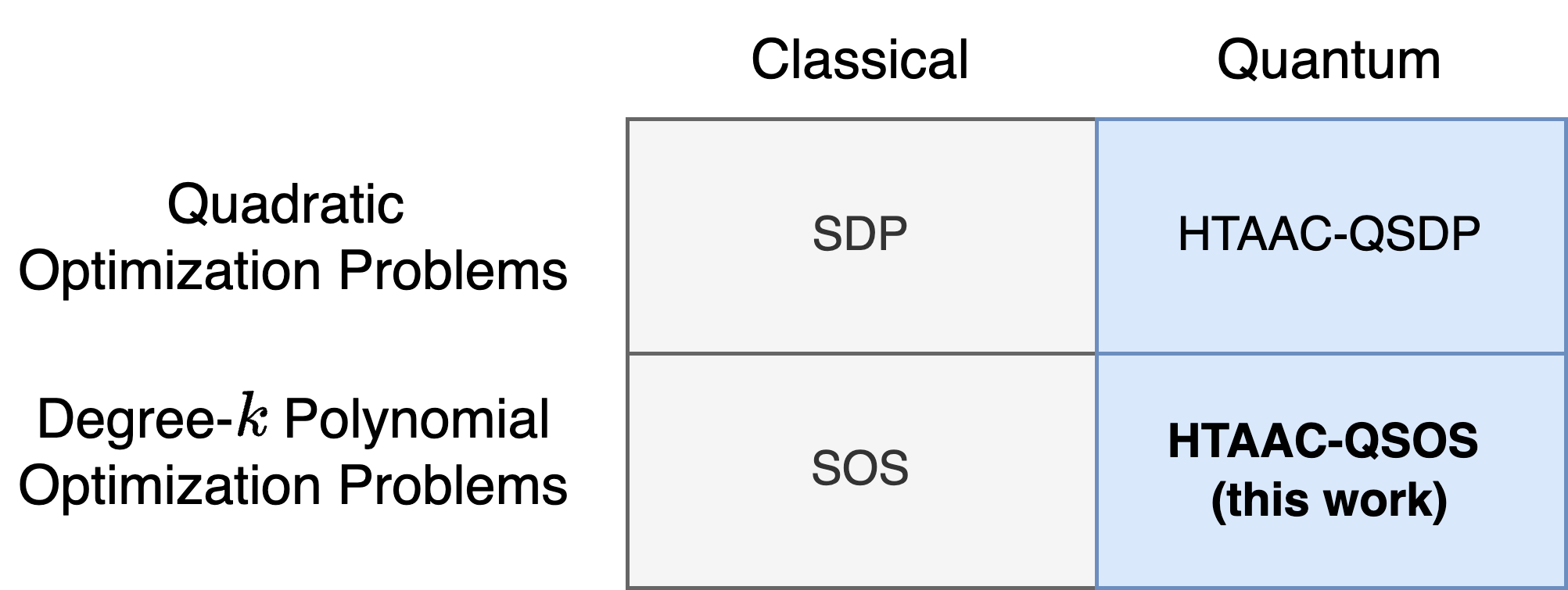
SDP for Max-2SAT and SOS programming for Max-SAT are standard classical relaxations that upper bound the solution. Figure 1 contextualizes these approximation algorithms. In addition, heuristic solvers (often based on local search or variational algorithms) aim to find feasible solutions to optimization problems quickly without guarantees on solution quality [25, 26, 29]. Since industrial applications often prioritize speed, these solvers may work well in practice but are frequently catered towards specific problems.
For concreteness, we focus our discussions of SDPs and HTAAC-QSDP on the problem Max-2SAT. We then describe how similar methodology may be extended to solve the Max-SAT via SOS. Despite our focus on SAT problems, we remind the reader that these optimization techniques readily generalize to other optimization problems [34, 9].
II.2 Max-2SAT and Semidefinite Programming
Max-2SAT presents a set of clauses, each containing two Boolean variables. The goal is to maximize the number of satisfiable clauses by optimally assigning the Boolean variables.
In this section, we detail the Goemans-Williamson (GW) approximation algorithm for Max-2SAT [28]. The GW algorithm is highly regarded due its favorable approximation ratio, which is conjectured to be optimal among polynomial-time algorithms. In particular, it is proven that the GW algorithm for Max-2SAT will deliver solutions with an expected value of at least 0.87856 times the optimal number of satisfied clauses. To approximate a solution using the GW algorithm, we first express Max-2SAT as a quadratic optimization problem. Then, we construct a relaxation of the problem as a semidefinite program (SDP). Finally, the solution to this SDP is rounded to produce a feasible, albeit potentially sub-optimal, solution to the Max-2SAT problem.
II.2.1 Max-2SAT
In this section we consider a Max-2SAT instance on boolean variables, whose values are represented as 222We note that is a deliberate choice to simplify notation when we introduce an auxiliary variable.. A Max-2SAT instance is a series of clauses written, without loss of generality, in Conjunctive Normal Form (CNF)333In Conjunctive Normal Form, clauses consist of literals (boolean variables and their negations) connected by the logical “or”, denoted by . These clauses are sometimes connected by the logical “and”, denoted by . Any propositional formula, or equation with some truth value, may be written in CNF form [35].. In CNF, a clause containing variables and is written as , where either or both of and may be replaced by their negations (denoted and , respectively) and denotes the logical “or”. Max-2SAT is the sum of all these clauses. We note that Max-SAT problems are similarly expressed, with variables per clause.
We define another set of variables that correspond to the boolean variables , writing such that for all . Notice that we have introduced the variable which has no corresponding boolean variable. This defines the truth value, that is, we say is true if and false if . While introducing is not necessary for a classical representation of the problem, we will see its importance for the quantum formulation later in this section.
To denote the truth value of a clause , we write if is true and if is false. Then, the truth value of and may be expressed as a function of :
| (1) |
The truth value of a clause is then given by
| (2) | ||||
The value of other clauses can be similarly expressed. If or are negated, then we replace the corresponding or with or . The truth value of all clauses of length-2 may then be expressed as a quadratic function. The maximum number of satisfiable clauses is therefore written as a maximization over where is the th clause in the given list of clauses. This is simply a linear combination of the quadratic terms seen in Eq. (2), yielding {maxi} ∑_i¡j (a_i,j (1 - y_i y_j) + b_i,j (1 + y_i y_j))) \addConstrainty_i ∈{ - 1, 1 }, ∀i ∈{0,…,N-1}, where and are scalar constants defined by the specific problem instance, and . While has a separate definition from other variables in , we can treat the same as once this quadratic function is determined.
In classical optimization, Eq. (II.2.1) is called a quadratic optimization problem. Other NP-hard problems such as MaxCut and MaxBisection may be similarly expressed as quadratic optimization problems. The conversion from the NP-hard problem instance to a quadratic optimization problem is done in polynomial time [28, 9].
We note that the polynomial objective function consists of only constant and quadratic (i.e., even-degree) terms. If we were to eliminate (for example, by fixing the convention that indicates as true and indicates as false for all ), then the resulting polynomial objective would also contain linear (odd-degree) terms. We find even-degree optimization problems favorable for their matrix forms, that is, their variable matrices can be defined as an outer product between vectors of variables. The role of is thus to formulate the polynomial objective with only even-degree terms. In general, any polynomial can be made even by introducing a variable analogous to .
II.2.2 Semidefinite Programming (SDP)
Semidefinite programming (SDP) and corresponding rounding procedures are standard techniques in classical optimization for bounding quadratic optimization problems such as Max-2SAT.
SDP is a class of convex optimization problems that aims to extremize a linear objective function over symmetric positive semidefinite matrices under a set of constraints. With diverse applications in control theory and combinatorial optimization [27, 8, 32, 33, 36], SDPs are often used to bound solutions to NP-hard maximization problems. Specifically, such NP-hard problems are expressed as quadratic optimizations (often over integer-valued variables), the encoding of which is relaxed such that optimization can take place over the space of positive semidefinite matrices. This new SDP matrix formulation provides a more tractable and relaxed form of the original problem; however, we emphasize that this relaxed form is not equivalent to the original NP-hard problem. Rather, the SDP relaxation strictly broadens the solution space, upper bounding the “feasible region” of the original NP-hard problem. The solution that corresponds to this upper bound is potentially outside the feasible region, so a rounding procedure returns it to the valid solution space. This yields an approximate lower bound (but possibly sub-optimal) solution.
In general, the relaxed SDP form of these optimization problems is given as {mini} X ∈S^+⟨W,X⟩ \addConstraint⟨A_μ, X⟩ = b_μ ∀μ≤M, where is an symmetric matrix encoding a specific problem instance, matrix and scalar describe problem constraints, and the angled brackets denote the matrix outer product
| (3) |
for some matrices and . These SDPs are exactly solvable using classical techniques such as interior point methods [8].
Returning to the Max-2SAT problem, we can reformulate the quadratic optimization form of Max-2SAT in Eq. (II.2.1) as an SDP. The variables are relaxed to take on a vector form , where represents the unit sphere in dimensions. Then, the quadratic form in Eq. (II.2.1) is relaxed to {maxi} ∑_i¡j (W_i,j^+ - v_i^T v_j W_i,j^-) \addConstraintv_i ∈S_N, ∀i ∈{0,…,N-1}, where and are matrix elements. The objective in Eq. (II.2.2), or number of satisfiable clauses, becomes where is an matrix of all ones, and . Eq. (II.2.2) is equivalent to the SDP {mini} X ∈S^+⟨W^-, X⟩ \addConstraintX_i,i = 1, ∀i ≤N.
We remark again that the SDP formulation is a relaxation of Max-2SAT. To obtain an approximate solution within the feasible space of the Max-2SAT instance, un-rounded solutions are rounded back to by determining which side of a random hyperplane they fall on. The resulting are substituted into Eq. (II.2.1) to determine the number of satisfied clauses in the rounded solution.
II.3 HTAAC-QSDP for Max-2SAT
In this section, we review the recently-proposed HTAAC-QSDP [1]. As a variational quantum analog to SDPs, HTAAC-QSDP finds heuristic solutions for problems with variables using only qubits, quantum measurements, and classical calculations. As with other variational quantum algorithms [23], the key elements of HTAAC-QSDP lie in the formulation of the loss function. The loss is determined using observables on the quantum state , and is minimized via the variational quantum circuit . Although HTAAC-QSDP is a general SDP technique, the precise loss function formulation is problem-dependent. In the following sections, we detail the application to Max-2SAT.
II.3.1 Evaluating the Objective
Beginning with the SDP formulation in Eq. (II.2.2), we replace the matrix with the density matrix , where in the computational basis. In particular, corresponds to for all , where we recall . The elements of represent , such that the quantum equivalent of Eq. (II.2.2) is 444To ensure that the dimensions of and match, may be “padded” with rows and columns of zeroes. In this work, the notation is the same for padded and non-padded versions of a matrix. {mini} ρ ⟨W^-, ρ⟩ \addConstraintρ_i,i = 2^-n, ∀i ≤N. The objective function may be written as as an expectation value
| (4) |
and may be used to generate a unitary ,
| (5) | ||||
Then, the value of the objective function may be approximated by using a Hadamard test to evaluate
| (6) |
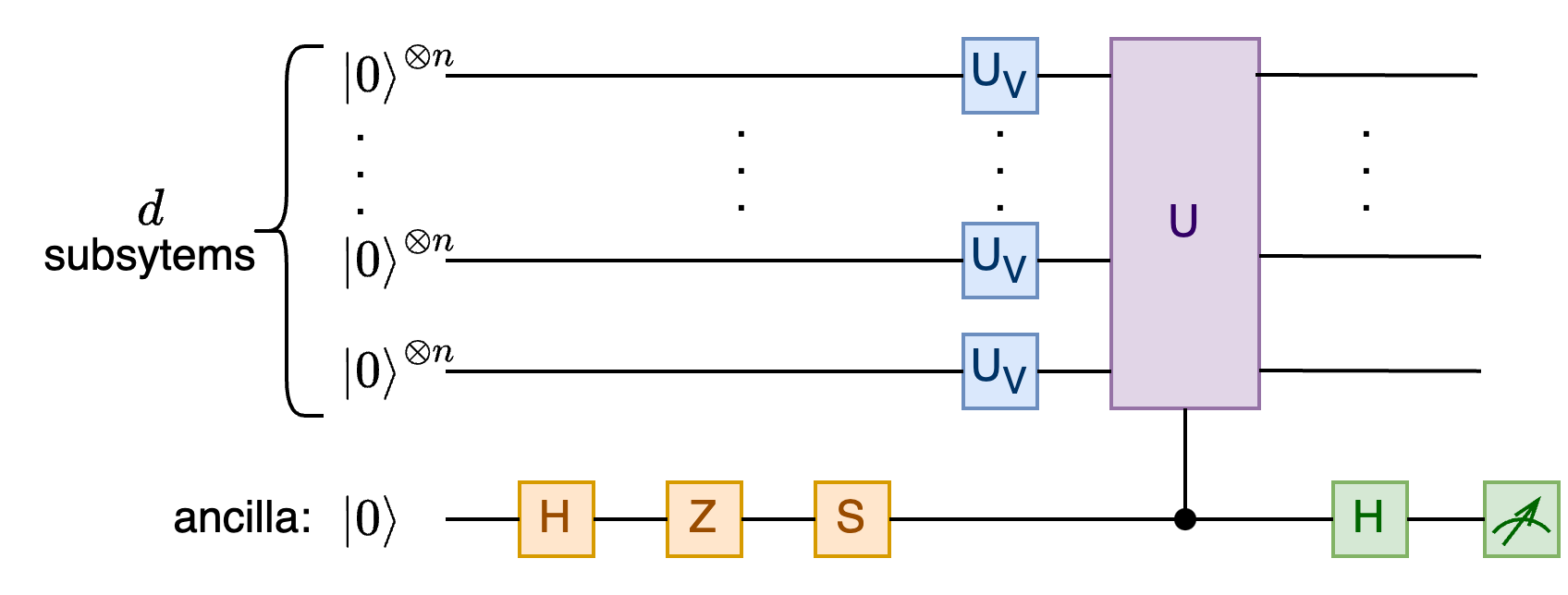
The Hadamard test is a quantum computing subroutine that estimates and other expectation values in the loss function. To generalize this subroutine we could simply replace with an arbitrary -qubit state and with an arbitrary -qubit unitary. The circuit used to execute the Hadamard test is shown in Figure 3, which shows that the Hadamard test uses only a single expectation value on an ancilla qubit
| (7) |
instead of the expectation values that would be otherwise required to fully characterize .
We note that the variational circuit is designed such that the elements of must be real. Thus, the objective is real, and Eq. (6) holds. Further discussion on the limits of this approximation is included in the original HTAAC-QSDP manuscript [1].
II.3.2 Approximate Amplitude Constraints
For Max-2SAT we wish to approximately enforce the constraint from Eq. (4). We note that enforcing is equivalent to enforcing up to normalization. This yields degrees of freedom, defined by unique equations555A unique set of equations is defined here as a set in which not equation can be deduced from other equations in the set. For example, are unique, but are not unique.. We can rewrite this set of equations using the following Pauli strings of length 1 to :
| (8) | ||||
The total number of equations is given by
| (9) |
Each of the Pauli strings in Eq. (8) yields an equation , for .
From Eq. (9), exactly enforcing the constraint requires observables. To avoid this, Patti et al. [1] propose approximate amplitude constraints. We approximately enforce by truncating Eq. (9) at , such that we only consider the Pauli strings up to length 2. All other terms give an extra degree of freedom (d.o.f.). This series may be truncated at higher to make the approximation more precise, in exchange for less-favorable polynomial scaling. The effect of this truncation is further explored in the original HTAAC-QSDP paper [1].
Since this method is approximate, HTAAC-QSDP includes an additional component to supplement the above Pauli string constraints. We introduce a diagonal matrix and a “population-balancing” unitary
| (10) | ||||
This helps to offset any asymmetric weights, and the expectation value of this unitary may be estimated using a Hadamard test.
II.3.3 The Loss Function
All three elements – the objective function, population-balancing unitary, and Pauli strings – may be combined as a single loss function to be minimized. The loss function is given by
| (11) |
The first term results from the Hadamard test used to estimate the objective function, the second term represents the set of Pauli strings , and the third term is from the Hadamard test used to estimate the population-balancing unitary. The second and third terms make up our approximate amplitude constraints, and are weighed by a Lagrange multiplier .
II.3.4 Retrieving Solutions
Once the loss is minimized, there are two ways to retrieve solutions from the resulting quantum state. One method uses sample-efficent estimation (SEE) and yields an un-rounded solution. Another method requires full state tomography (FST), but its complexity does not depend on the degree of the polynomial and the result mimics classical rounded solutions.
SEE may be used to directly estimate a solution from with the quantum analog to Eq. (LABEL:eqn:max2sat_obj_func),
| (12) |
The first term represents constant terms, where is the equal superposition of all states. This may be evaluated using the Hadamard test, where the unitary is acting on the quantum state . We evaluate
| (13) | ||||
The second term is equivalent to quadratic terms in the objective. Thus, the solution given by SEE is
| (14) |
While this solution is un-rounded, it is a good approximation of a rounded solution in the limit of well-behaved constraints. When the constraints are exactly enforced, the solution approaches the optimal rounded solution.
II.4 Max-SAT and Sum-of-Squares Programming
In this section, we describe how Max-SAT may be expressed as a polynomial optimization problem and approximated with classical sum-of-squares (SOS) programming. We first consider an extension from Max-2SAT to Max-3SAT.
II.4.1 The Polynomial Optimization Problem
In Max-3SAT, clauses are written in the form , where any of , , and may be replaced by their negations. By incorporating analogously to Max-2SAT, the truth value of the clause is expressed as
| (15) | ||||
The value of other clauses can be similarly expressed. If any of , , and are negated, then we replace the corresponding , , or with , , or . Once these polynomials are formulated for every clause, may be treated identically to . The truth value of all clauses of length-3 may then be expressed as a degree-4 polynomial. The maximum number of satisfiable clauses is therefore written as a maximization over , where is the th clause in the given list of clauses. This is a linear combination of the quadratic and degree-4 terms in Eq. (15),
| (16) | ||||
where , , , and are scalar constants defined by the specific problem instance, and . The result is a non-convex degree-4 polynomial objective, consisting of only even-degree terms.
We note that we may obtain a degree-3 polynomial if we eliminate (for example, by fixing the convention that indicates as true and indicates as false for all ). Classical SOS can target degree-3 polynomials, but formulating polynomials with even-degree terms using is more suitable to our quantum approach.
To generalize this formulation to Max-SAT, we introduce some notation. Max-SAT may be formulated as a degree- polynomial without , and as a degree-2 polynomial with where . The maximum degree of the polynomial objective is , and we also we define such that denotes the degree of individual terms in the objective. For example, in Max-3SAT we have a degree-4 polynomial objective, and therefore . Within this degree-4 polynomial we have constant, degree-2, and degree-4 terms, such that , , and respectively. Because constant terms do not impact the solution of an optimization problem, they are dropped and . Since any polynomial can be made to have only even-degree terms using and our proposed algorithm makes use of the even-degree characteristic, we focus on degree-2 polynomials in our discussions.
II.4.2 Sum-of-Squares (SOS)
SOS programming is a core discipline in operations research [30]. In this section, we provide a cursory overview of the relevant SOS formulae, providing a more detailed treatment in the Appendix.
SOS programming determines whether a degree- polynomial function , where , can be factored as a sum of squares. We express as
| (17) |
where is a symmetric matrix and
| (18) |
is a “polynomial basis”. This basis enables the generalization to higher-degree polynomials. The matrix can be interpreted as a “weight” matrix of coefficients. It is proven that is a sum of squares if and only if is positive semidefinite. SOS is therefore solvable by SDP [30].
In the context of polynomial optimization, we can define where is the polynomial objective and is a real number. Writing as SOS is an algebraic certificate of nonnegativity, that is, . Then, , and we may derive an upper bound on .
In the context of Max-SAT, a problem instance is expressed as degree- polynomial optimization, which is then written as SOS to determine an upper bound. Similarly to the SDP approach, a rounding procedure may be used to identify a feasible solution and a lower bound. Rounding procedures typically involve random sampling similar to that in the GW algorithm. Details and an example are provided in Appendix A.
II.5 Approximation Guarantees and Caveats
To further contextualize the SDP and SOS approximation methods we can consider the simplest approximation algorithm for Max-SAT: random guess, where each variable is assigned to be true with probability . This yields a -approximation algorithm, that is, the approximated solution is expected to be at least times the optimum solution [9]. This is the baseline guarantee, and we hope to obtain solutions that are closer to the optimal with methods such as SDP and SOS.
While SOS provides a strict upper bound on the objective function, the rounded SOS solution has no approximation ratio guarantee. The approximation ratio given by the GW algorithm for Max-2SAT is lost in the generalization to Max-SAT. Furthermore, the rounding procedure for SOS suffers from a lack of algebraic consistency. Algebraic consistency refers to the requirement that the element representing and the element representing multiply to equal the element representing in the polynomial basis (Eq. (18)) [38].
For a polynomial objective function of degree- and variables, SOS requires the manipulation of matrices with dimension due to the polynomial basis . While an improvement over the brute force solution, this renders SOS intractable for large problem sizes, such as those found in industrial applications and scientific research.
III The Proposed Algorithm: HTAAC-QSOS
In this section we present our proposed algorithm: an SOS-inspired quantum metaheuristic for polynomial optimization with the Hadamard test and approximate amplitude constraints (HTAAC-QSOS). As a continuation of the previous discussion, we apply HTAAC-QSOS to Max-3SAT, simulating the algorithm and comparing it against classical benchmarks. We also show how HTAAC-QSOS for Max-3SAT generalizes to Max-SAT. Finally, we describe a generalized overview of HTAAC-QSOS for any polynomial optimization problem.
III.1 HTAAC-QSOS for Max-3SAT
III.1.1 Evaluating the Objective
The polynomial objective function for Max-3SAT (Eq. (16)) may be rewritten as
| (19) | ||||
where
| (20) | ||||
The variables are encoded using computational basis states, identically to HTAAC-QSDP. The objective function becomes
| (21) | |||
| (22) |
where is an matrix of all ones and is an matrix of all ones. The problem becomes {mini} ρ⏞⟨W^-,(1), ρ⟩^degree-2 terms + ⏞⟨W^-,(2), ρ⊗ρ⟩^degree-4 terms \addConstraintρ_i,i = 2^-n, ∀i ≤N where the objective function is the sum of two expectation values,
| (23) | ||||
A core contribution of this work lies in the introduction of the product state for degree-4 terms. The product state is a tensor product over two identical states , such that its elements represent the degree-4 terms . This is the quantum analog to the polynomial basis in SOS. However, while SOS programming is solved with SDPs by including the polynomial basis as additional constraints, our proposed algorithm naturally preserves these constraints by encoding solutions as product states. HTAAC-QSOS therefore requires no additional constraints apart from those included in the original problem.
In terms of implementation, we propose a “multiple register” approach. Each “register” is an identical -qubit quantum subsystem. Degree-2 terms are evaluated with a Hadamard test on a single register and a unitary , similarly to Max-2SAT,
| (24) |
To evaluate degree-4 terms in the objective function, two identical copies of the state are prepared on two registers. A Hadamard test is implemented by operating on both registers with a larger -qubit unitary i.e., ,
| (25) |
The circuit diagram for these two Hadamard tests is shown in Figure 3, where and respectively.
III.1.2 Approximate Amplitude Constraints
We want to enforce the constraint for all . In Section II.3.2, we describe how we may approximately enforce this constraint using Pauli strings and a population-balancing unitary. Since we encode the objective function using product states, we do not require any additional constraints. Specifically, we write Pauli string equations
| (26) | ||||
and define the population-balancing unitary
| (27) | ||||
The population-balancing unitary has the same formulation as described in Section II.3.2, but with in place of . The purpose of the population-balancing unitary is to approximate the frequency at which a variable appears, and the larger matrix is therefore not required.
III.1.3 Retrieving Solutions
Extending the SEE method in Section II.3.4, we evaluate the un-rounded solution using the quantum analog of Eq. (22)
| (28) | ||||
The first term is estimated using a Hadamard test with unitary acting on state , and the second term is estimated using a Hadamard test acting on state . The third and fourth terms are part of the objective function in Section III.1.1. The un-rounded solution for Max-3SAT is
| (29) | ||||
To obtain the rounded solution we require FST, and follow the same procedure outlined in Section II.3.4.
III.2 Simulating HTAAC-QSOS for Max-3SAT
We test our proposed algorithm by simulating HTAAC-QSOS for Max-3SAT on a classical system and benchmarking results against classical SOS and heuristic methods. To present our results, we define observed performance, or the ratio between the HTAAC-QSOS result and the classical benchmark result for a given problem instance. In Tables 1 and 2, this ratio is calculated and averaged over several instances of the same size.
III.2.1 SOS vs. HTAAC-QSOS
To test the performance of HTAAC-QSOS against SOS, we generate several Max-3SAT instances by drawing variables from a uniform distribution and removing clauses with repeating variables. The SOS techniques [31] are used to obtain classical solutions. We choose problems with 20 variables each because they may be approximated by SOS within reasonable time.
We remark that SOS often yields very tight upper bounds, frequently finding the optimal solution [38, 9]. However, since these upper bounds do not necessarily correspond to feasible solutions, we use a rounding procedure (described in Appendix A.2) to return the SDP solutions to the feasible region. We use the rounded result as a classical benchmark. The rounded result is typically within 92% to 96% of the upper bound for the problem sizes used [38]. Results are provided in Table 1.
| Max-3SAT Problem Size | HTAAC-QSOS (SEE) | HTAAC-QSOS (FST) | |||
|---|---|---|---|---|---|
| # of var. | # of clauses | Best Found | Average | Best Found | Average |
| 20 | 80 | 1.040 | 1.039 | 1.084 | 1.078 |
| 100 | 1.042 | 1.041 | 1.084 | 1.079 | |
| 120 | 1.025 | 1.024 | 1.071 | 1.067 | |
| 140 | 1.027 | 1.026 | 1.079 | 1.076 | |
| 160 | 1.004 | 1.003 | 1.050 | 1.045 | |
| 180 | 1.001 | 1.008 | 1.047 | 1.044 | |
Both the SEE and rounded FST objective values from HTAAC-QSOS are consistently greater than that of the rounded classical SOS solution, despite encoding only a rough approximation of the problem. Notably, the un-rounded SEE objectives are less than their corresponding rounded FST objectives, implying favorable rounding behavior. We hypothesize that this rounding behavior can be attributed to the algebraic consistency maintained by HTAAC-QSOS. Algebraic consistency refers to the requirement that the element representing and the element representing multiply to equal the element representing in the polynomial basis. This property is naturally preserved by the product states used in HTAAC-QSOS, but not by the rounding procedure in classical SOS. This results in a much simpler rounding scheme for HTAAC-QSOS, and one that yields heuristics that are closer to the optimal solution, based on our simulation result.
Moreover, in SDP relaxations, the rank of the solution may serve as an indicator of solution quality. Many polynomial optimization problems yield a natural SDP relaxation. If the SDP relaxation has a rank-1 solution, then the relaxation is exact, and there is no gap between the upper bound and the rounded solution. Intuitively, this suggests that rank-1 solutions are more desirable [36]. SDP relaxations often yield full-rank solutions. The solution to HTAAC-QSOS is always a pure state and therefore is rank-1, suggesting that HTAAC-QSOS may result in solutions that yield a smaller optimality gap when rounded.
III.2.2 Classical Heuristic vs. HTAAC-QSOS
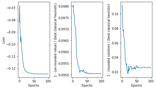
To gauge the performance of HTAAC-QSOS for larger problems, we draw instances with 70 to 110 variables from the 2016 MaxSAT evaluation [26]. Since classical SOS is intractable for larger problems, the best known solutions are given by the winning heuristic solutions from the MaxSAT evaluation. These solvers primarily leverage local search algorithms and problem-specific heuristics. Like HTAAC-QSOS, these solvers prioritize speed over approximation ratio guarantees. The observed performance is therefore calculated with respect to these solutions, and averaged over instances of the same size given by the MaxSAT evaluation. The results are given in Table 2, and Figure 4 shows loss and observed performance over 100 training epochs for a Max-3SAT instance with 110 variables and 1100 clauses.
| Max-3SAT Instance | HTAAC-QSOS (SEE) | HTAAC-QSOS (FST) | |||
|---|---|---|---|---|---|
| # of var. | # of clauses | Best Found | Mean | Best Found | Mean |
| 70 | 700 | 0.911 | 0.903 | 0.985 | 0.978 |
| 800 | 0.909 | 0.901 | 0.984 | 0.981 | |
| 900 | 0.910 | 0.909 | 0.986 | 0.979 | |
| 90 | 700 | 0.899 | 0.898 | 0.978 | 0.969 |
| 800 | 0.903 | 0.902 | 0.979 | 0.972 | |
| 900 | 0.906 | 0.905 | 0.977 | 0.966 | |
| 1000 | 0.911 | 0.910 | 0.980 | 0.973 | |
| 1100 | 0.908 | 0.907 | 0.978 | 0.972 | |
| 1200 | 0.902 | 0.901 | 0.976 | 0.970 | |
| 1300 | 0.906 | 0.905 | 0.978 | 0.971 | |
| 110 | 700 | 0.906 | 0.905 | 0.972 | 0.961 |
| 800 | 0.909 | 0.908 | 0.974 | 0.961 | |
| 900 | 0.900 | 0.899 | 0.979 | 0.970 | |
| 1000 | 0.907 | 0.906 | 0.973 | 0.963 | |
| 1100 | 0.908 | 0.907 | 0.981 | 0.971 | |
The un-rounded SEE solutions’ objective value are within ten percent of the objectives from the best classical heuristic, and the corresponding objectives of the rounded FST solutions are within three percent. Figure 4 shows that the un-rounded objectives, rounded objectives, and loss are strongly correlated. Un-rounded solutions consistently yield rounded FST solutions that are close to the optimal.
While these initial simulations of HTAAC-QSOS for Max-3SAT yield objectives that are slightly less than those given by existing classical heuristic solvers, the advantage of HTAAC-QSOS lies in its generalizability. Classical incomplete solvers may be specifically tailored to Max-SAT, but the HTAAC-QSOS framework can be generalized to any polynomial optimization problem. While HTAAC-QSOS works with even degree polynomials, this is without loss of generality because odd-degree polynomials can be made even through the introduction of an auxiliary variable such as [8, 9].
III.3 HTAAC-QSOS for Max-SAT
The proposed SOS-inspired approach for Max-3SAT may be easily applied to Max-SAT. The number of qubits required scales linearly with , and the number of constraints is independent of .
III.3.1 Evaluating the Objective
Max-SAT can be expressed as a degree-2 polynomial optimization problem, where is the maximum degree of the polynomial objective666We remind the reader that Max-SAT can also be expressed as a degree- polynomial optimization problem, but we introduce here to make the polynomial even and therefore simpler to address with our quantum approach.. The polynomial consists of only even-degree monomial terms of degree-, such that . The generalized problem is written as {mini} ρ∑_d = 1^D ⟨W^-,(d), ρ^⊗d⟩ \addConstraintρ_i,i = 2^-n, ∀i ≤N where the objective function is a sum of expectation values
| (55) |
and we define to simplify notation.
Each encodes terms of degree- and can be estimated using the Hadamard test,
| (56) |
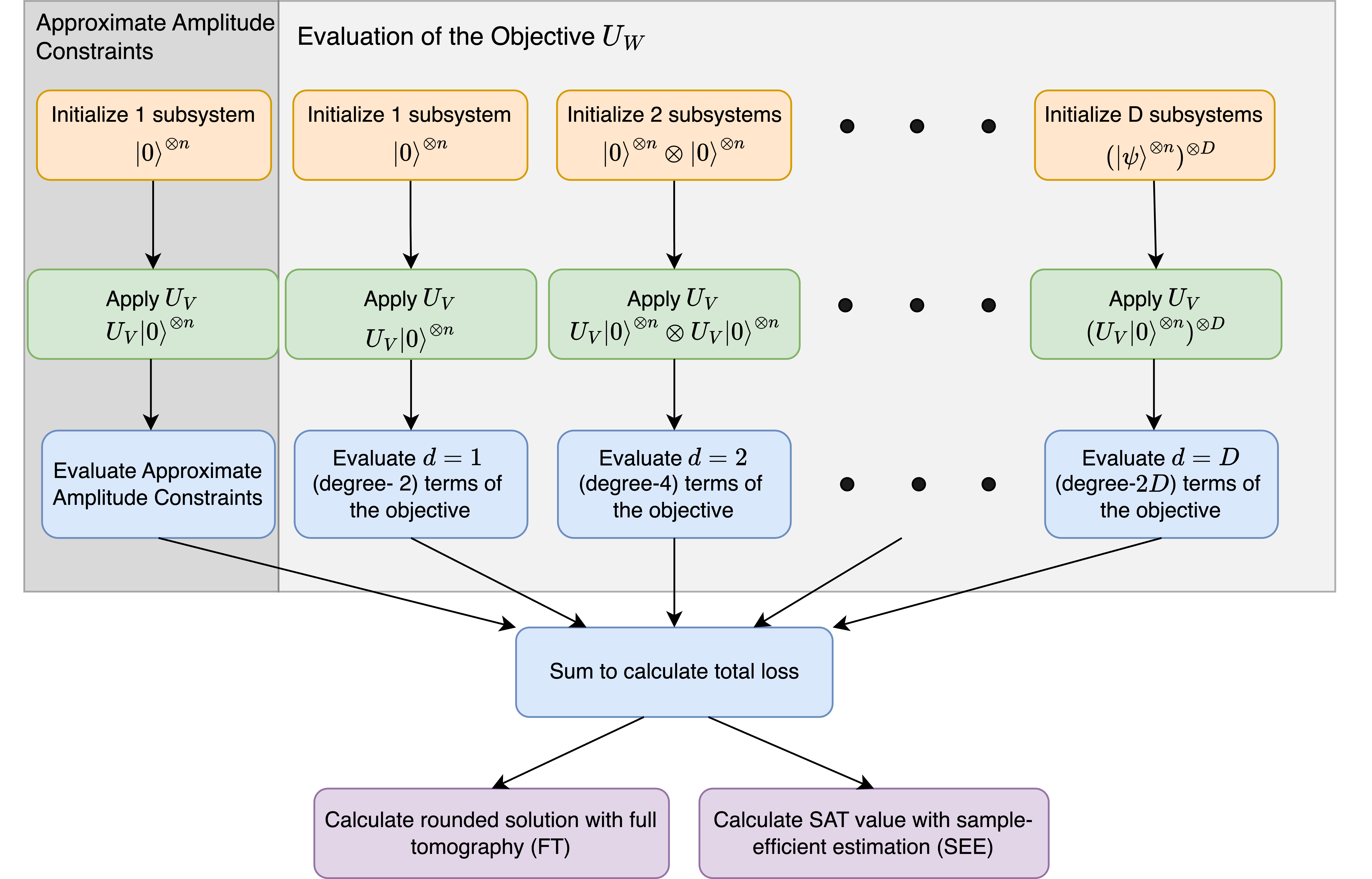
where (see Figure 3). To be specific, we evaluate all terms of degree- by first simultaneously and separately preparing identical copies of . Then, we use the -qubit unitary to conduct the Hadamard test upon the entire quantum system – all copies. Repeating this for all possible values of , we can evaluate all terms in the objective function. We therefore require a total of Hadamard tests and qubits to estimate the objective function.
This is our “multiple register” approach, where each register of qubits hosts a copy of . This allows us to generalize the original HTAAC-QSDP framework for degree- polynomial optimization with time and resource complexity.
III.3.2 Approximate Amplitude Constraints
The Pauli strings and the population-balancing unitary are formulated identically to those in Max-3SAT (see Section III.1.2), since the equality constraint in the optimization problem is the same. Thus, the number of measurements required to approximately enforce constraints is independent of .
III.3.3 Retrieving Solutions
The un-rounded SEE solution for Max-3SAT in Eq. (29) can be generalized to
| (57) | ||||
where we recall and each term may be evaluated with a Hadamard test. We therefore require Hadamard tests to determine this un-rounded solution.
The second rounding method follows the same procedure described in Section II.3.4. This method is the same for all values of , and involves full state tomography the -qubit subsystem.
III.4 HTAAC-QSOS for Polynomial Optimization
We recall that any degree- polynomial optimization can be made into a degree-2 polynomial with terms of degree 2, where , using a auxiliary variable [8, 9]. For the quadratic optimization problems addressed with HTAAC-QSDP, and . In the polynomial optimization problems we address with our proposed HTAAC-QSOS, we allow and . Terms of degree-2 may be approximated with quantum subsystems of qubits each. Therefore, we require qubits to estimate the objective function. Furthermore, the property of Pauli strings to form a complete basis suggests that they may be used to enforce any linear equality constraint. To retrieve the solutions, the SEE and FST methods may be generalized. The SEE method requires Hadamard tests, namely, one for value of . The FST rounding method for polynomial optimization over binary variables requires full state tomography of a -qubit subsystem, but is constant in .
IV Conclusions and Outlook
In this manuscript, we propose a SOS-inspired quantum metaheuristic for polynomial optimization (HTAAC-QSOS), that extends the recently proposed HTAAC-QSDP algorithm [1] using classical sum-of-squares (SOS). This technique yields a heuristic that is scalable to challenging and useful problems, such as those found in operations research and similar research applications. Moreover, HTAAC-QSOS is generalizable, and scales linearly with the degree of the polynomial. Notably, HTAAC-QSOS exhibits superior rounding behavior compared to classical SOS methods, likely due to its preservation of algebraic consistency through product state encoding.
In our study of Max-SAT, we emphasize as the degree of the polynomial objective increases, only the evaluation of the objective changes. In fact, the number of approximate amplitude constraints required in Max-SAT is independent of the degree of the polynomial objective. While classical SOS requires additional constraints with the increase of , these constraints are naturally conserved by the product state encoding in HTAAC-QSOS. If the Hadamard tests are conducted sequentially on a set of registers, then the time and resource complexities of HTAAC-QSOS are therefore only linear in , whereas the less-favorable complexities of classical SOS are polynomial. Alternatively, if we want Hadamard tests to be conducted simultaneously on more registers, then HTAAC-QSOS is constant in time and quadratic in resources (i.e., qubits) with respect to . HTAAC-QSOS thus has the potential to address a broader class of polynomial optimization problems than previous quantum approaches or problem-specific classical heuristics, while maintaining better scaling than classical SOS methods as the degree of the polynomial increases.
The generalization to any polynomial optimization may be tested by applying the HTAAC-QSOS approach to other families of polynomial optimization problems, including those that are optimized over continuous variables. In these continous cases, the rounding step of the FST solution method may not be required. One possible application is in quantum chemistry, where the SOS hierarchy (i.e., the reduced density matrix method) is used to study weak coupling perturbation theory [39]. SOS is also used as an approach towards the best separable quantum state problem [40].
Additionally, the high performance of the FST rounding method in classical simulations suggests that HTAAC-QSOS may be a strong candidate for a quantum-inspired algorithm. Since the circuit does not need to be implemented on qubits, the Hadamard test is not required, and we may directly evaluate the objective function using the weight matrix.
Acknowledgements R.B. was supported by NSF CCF (grant #1918549). S.F.Y. would like to thank the NSF via QIdeas HDR (OAC-2118310) and the CUA PFC (PHY-2317134).
References
- Patti et al. [2023] T. L. Patti, J. Kossaifi, A. Anandkumar, and S. F. Yelin, Quantum goemans-williamson algorithm with the hadamard test and approximate amplitude constraints, Quantum 7, 1057 (2023).
- Biamonte et al. [2017] J. Biamonte, P. Wittek, N. Pancotti, P. Rebentrost, N. Wiebe, and S. Lloyd, Quantum machine learning, Nature 549, 195–202 (2017).
- Cao et al. [2019] Y. Cao, J. Romero, J. P. Olson, M. Degroote, P. D. Johnson, M. Kieferová, I. D. Kivlichan, T. Menke, B. Peropadre, N. P. D. Sawaya, S. Sim, L. Veis, and A. Aspuru-Guzik, Quantum chemistry in the age of quantum computing, Chemical Reviews 119, 10856–10915 (2019).
- Montanaro [2016] A. Montanaro, Quantum algorithms: an overview, npj Quantum Information 2, 1–8 (2016).
- Preskill [2018] J. Preskill, Quantum computing in the nisq era and beyond, Quantum 2, 79 (2018).
- Korte and Vygen [2018] B. Korte and J. Vygen, Introduction, in Combinatorial Optimization: Theory and Algorithms (Springer, Berlin, Heidelberg, 2018) p. 1–13.
- Berg et al. [2019] J. Berg, A. Hyttinen, and M. Järvisalo, Applications of maxsat in data analysis, in EPiC Series in Computing, Vol. 59 (EasyChair, 2019) p. 50–64.
- Vandenberghe and Boyd [1996] L. Vandenberghe and S. Boyd, Semidefinite programming, SIAM Review 38, 49–95 (1996).
- Vazirani [2001] V. V. Vazirani, Approximation Algorithms (Springer Link, 2001).
- Brandão et al. [2022] F. G. S. L. Brandão, R. Kueng, and D. S. França, Faster quantum and classical sdp approximations for quadratic binary optimization, Quantum 6, 625 (2022).
- Brandao and Svore [2017] F. G. Brandao and K. M. Svore, Quantum speed-ups for solving semidefinite programs, in 2017 IEEE 58th Annual Symposium on Foundations of Computer Science (FOCS) (2017) p. 415–426.
- Apeldoorn et al. [2020] J. v. Apeldoorn, A. Gilyén, S. Gribling, and R. d. Wolf, Quantum sdp-solvers: Better upper and lower bounds, Quantum 4, 230 (2020).
- van Apeldoorn and Gilyén [2019] J. van Apeldoorn and A. Gilyén, Improvements in quantum sdp-solving with applications, in DROPS-IDN/v2/document/10.4230/LIPIcs.ICALP.2019.99 (Schloss Dagstuhl – Leibniz-Zentrum für Informatik, 2019).
- Ebadi et al. [2022] S. Ebadi, A. Keesling, M. Cain, T. T. Wang, H. Levine, D. Bluvstein, G. Semeghini, A. Omran, J.-G. Liu, R. Samajdar, X.-Z. Luo, B. Nash, X. Gao, B. Barak, E. Farhi, S. Sachdev, N. Gemelke, L. Zhou, S. Choi, H. Pichler, S.-T. Wang, M. Greiner, V. Vuletić, and M. D. Lukin, Quantum optimization of maximum independent set using rydberg atom arrays, Science 376, 1209–1215 (2022).
- Brandão et al. [2019] F. G. S. L. Brandão, A. Kalev, T. Li, C. Y.-Y. Lin, K. M. Svore, and X. Wu, Quantum sdp solvers: Large speed-ups, optimality, and applications to quantum learning, in DROPS-IDN/v2/document/10.4230/LIPIcs.ICALP.2019.27 (Schloss Dagstuhl – Leibniz-Zentrum für Informatik, 2019).
- Patel et al. [2021] D. Patel, P. J. Coles, and M. M. Wilde, Variational quantum algorithms for semidefinite programming, arXiv 10.48550/arXiv.2112.08859 (2021), arXiv:2112.08859 [quant-ph].
- Albash and Lidar [2018] T. Albash and D. A. Lidar, Adiabatic quantum computation, Reviews of Modern Physics 90, 015002 (2018).
- Farhi et al. [2014] E. Farhi, J. Goldstone, and S. Gutmann, A quantum approximate optimization algorithm, arXiv 10.48550/arXiv.1411.4028 (2014).
- Farhi et al. [2000] E. Farhi, J. Goldstone, S. Gutmann, and M. Sipser, Quantum computation by adiabatic evolution, arXiv 10.48550/arXiv.quant-ph/0001106 (2000).
- Gibney [2017] E. Gibney, D-wave upgrade: How scientists are using the world’s most controversial quantum computer, Nature 541, 447–448 (2017).
- Kadowaki and Nishimori [1998] T. Kadowaki and H. Nishimori, Quantum annealing in the transverse ising model, Physical Review E 58, 5355–5363 (1998).
- Arrazola et al. [2021] J. M. Arrazola, V. Bergholm, K. Brádler, T. R. Bromley, M. J. Collins, I. Dhand, A. Fumagalli, T. Gerrits, A. Goussev, L. G. Helt, J. Hundal, T. Isacsson, R. B. Israel, J. Izaac, S. Jahangiri, R. Janik, N. Killoran, S. P. Kumar, J. Lavoie, A. E. Lita, D. H. Mahler, M. Menotti, B. Morrison, S. W. Nam, L. Neuhaus, H. Y. Qi, N. Quesada, A. Repingon, K. K. Sabapathy, M. Schuld, D. Su, J. Swinarton, A. Száva, K. Tan, P. Tan, V. D. Vaidya, Z. Vernon, Z. Zabaneh, and Y. Zhang, Quantum circuits with many photons on a programmable nanophotonic chip, Nature 591, 54–60 (2021).
- Cerezo et al. [2021] M. Cerezo, A. Arrasmith, R. Babbush, S. C. Benjamin, S. Endo, K. Fujii, J. R. McClean, K. Mitarai, X. Yuan, L. Cincio, and P. J. Coles, Variational quantum algorithms, Nature Reviews Physics 3, 625–644 (2021).
- Bittel and Kliesch [2021] L. Bittel and M. Kliesch, Training variational quantum algorithms is np-hard, Physical Review Letters 127, 120502 (2021).
- Cai and Zhang [2020] S. Cai and X. Zhang, Pure maxsat and its applications to combinatorial optimization via linear local search, in Principles and Practice of Constraint Programming, edited by H. Simonis (Springer International Publishing, Cham, 2020) p. 90–106.
- of the 19th International Conference on Theory and of Satisfiability Testing [2016] O. of the 19th International Conference on Theory and A. of Satisfiability Testing, The homepage of eighth max-sat evaluation, http://maxsat.ia.udl.cat/introduction/ (2016).
- Parrilo [2003] P. A. Parrilo, Semidefinite programming relaxations for semialgebraic problems, Mathematical Programming 96, 293–320 (2003).
- Goemans and Williamson [1995] M. X. Goemans and D. P. Williamson, Improved approximation algorithms for maximum cut and satisfiability problems using semidefinite programming, Journal of the ACM 42, 1115–1145 (1995).
- Hickey and Bacchus [2022] R. Hickey and F. Bacchus, Large neighbourhood search for anytime maxsat solving, in Proceedings of the Thirty-First International Joint Conference on Artificial Intelligence, IJCAI 2022, Vienna, Austria, 23-29 July 2022, edited by L. D. Raedt (ijcai.org, 2022) pp. 1818–1824.
- [30] A. A. Ahmadi, Sum of squares (sos) techniques: An introduction.
- Prajna et al. [2002] S. Prajna, A. Papachristodoulou, and P. Parrilo, Introducing sostools: a general purpose sum of squares programming solver, in Proceedings of the 41st IEEE Conference on Decision and Control, 2002., Vol. 1 (2002) p. 741–746 vol.1.
- Harrach [2022] B. Harrach, Solving an inverse elliptic coefficient problem by convex non-linear semidefinite programming, Optimization Letters 16, 1599–1609 (2022).
- Gepp et al. [2020] A. Gepp, G. Harris, and B. Vanstone, Financial applications of semidefinite programming: a review and call for interdisciplinary research, Accounting and Finance 60, 3527–3555 (2020).
- Cook [1971] S. A. Cook, The complexity of theorem-proving procedures, in Proceedings of the third annual ACM symposium on Theory of computing, STOC ’71 (Association for Computing Machinery, New York, NY, USA, 1971) p. 151–158.
- Howson [1997] C. Howson, Logic with Trees: An Introduction to Symbolic Logic (Routledge, New York, 1997).
- Lemon et al. [2016] A. Lemon, A. M.-C. So, and Y. Ye, Low-rank semidefinite programming: Theory and applications, Foundations and Trends in Optimization 2, 1–156 (2016).
- Hakemi et al. [2024] S. Hakemi, M. Houshmand, E. KheirKhah, and S. A. Hosseini, A review of recent advances in quantum-inspired metaheuristics, Evolutionary Intelligence 17, 627–642 (2024).
- van Maaren et al. [2008] H. van Maaren, L. van Norden, and M. J. H. Heule, Sums of squares based approximation algorithms for max-sat, Discrete Applied Mathematics 156, 1754–1779 (2008).
- Hastings [2024] M. B. Hastings, Perturbation theory and the sum of squares, arXiv (2024), arXiv:2205.12325 [cond-mat, physics:hep-th, physics:quant-ph].
- Doherty et al. [2004] A. C. Doherty, P. A. Parrilo, and F. M. Spedalieri, Complete family of separability criteria, Physical Review A 69, 022308 (2004).
Appendix A Sum-of-Squares (SOS) and Rounding Procedures
In this section of the appendix, we provide more details on the sum-of-squares (SOS) method as well as its rounding procedures.
A.1 SOS Hierarchy
While there exist several relaxation algorithms and rounding procedures used to approximate solutions to Max-SAT and similar problems, we choose SOS as the most standard and systematic method as a classical benchmark for our algorithm.
Let be a multivariate polynomial, where denotes the variables . The goal of classical SOS is to write in such a way that the nonnegativity of becomes obvious. Specifically, the existence of an SOS decomposition
| (58) |
where are some polynomials in , is an algebraic certificate of nonnegativity.
The SOS hierarchy is a hierarchy is convex relaxations, ordered with increasing power and computational cost. The th level of the hierarchy corresponds to polynomial optimization problems with a degree- polynomial objective. The first level of the hierarchy, where , corresponds to an SDP for a quadratic optimization problem. To consider higher-degree polynomials, new variables and constraints must be introduced such that the problem may then be solved as a larger SDP with additional constraints. Specifically, we draw a connection between SOS and semidefinite matrices with the following theorem.
Theorem 1.
A degree-2 multivariate polynomial is a sum-of-squares if and only if there exists positive semidefinite matrix such that
| (59) |
where . The vector is the polynomial basis, and the matrix is called the Gram matrix.
A proof is provided by [30].
To show how SOS is applied to polynomial optimization problems, we consider a generic problem of the form {maxi} p(y) \addConstrainth_j(y) = 0, ∀j ∈{1, 2, …, M} where is a polynomial objective that is not necessarily convex, are equality constraints, and is the number of constraints. Using the given problem, we define a new polynomial777SOS is often used to determine a lower bound on the solution of the original problem. Here, we want to find an upper bound. To make the notation more straightforward, we introduced a factor of to in our formulation of .
| (60) |
where a real-valued variable, and is a polynomial with its degree limited by . If may be factored into a sum of squares for a some value of and some polynomials , we guarantee that . When the constraints are satisfied such that , we obtain such that forms an upper bound on . Formally, we want to obtain a tight upper bound bound on by solving {maxi} γ \addConstraintF(y) is SOS. Since we look for solutions where , the polynomials in Eq. (60) function as additional degrees of freedom that allow tighter upper bounds.
As a very simple example, let us consider a Max-3SAT problem with two clauses: and . The equivalent polynomial optimization problem is {maxi} 14(y_0y_3 - y_1 y_2 + y_0y_1y_2y_3 ) + 74 \addConstrainty_i^2 = 1 ∀i ∈{0, 1, 2, 3} where the objective function is formulated using Eq. (15). The result may be approximated using the SOS in Eq. (A.1), where
| (61) | ||||
This is results in a polynomially-sized SDP by Theorem 1. Specifically, we define
| (62) |
and determine as a function of and the coefficients of such that is SOS, that is, . In this way, the problem becomes the SDP {maxi} Q ∈S^+⟨W, Q⟩ \addConstraint⟨bb^T, Q⟩ = F(y) where is defined such that . Solving the SDP, we obtain an upper bound , as we expect.
A.2 Rounding Procedures
The rounding procedure used in our SOS solution is equivalent one of the rounding procedures described by van Maaren et al. [38], and the steps are as follows. It can be shown that the optimal solution of the SOS method described in the previous section has an eigenvalue zero. We determine the orthogonal basis of eigenvectors of that have eigenvalue zero, such that for . Then, we randomly sample a vector from the -dimensional unit sphere and use this to generate a linear combination of these eigenvectors,
| (63) |
The elements of are rounded to or , and the results are used as the solution to the original polynomial optimization problem.
We note that the vectors for do not preserve algebraic consistency, that is, the product of elements corresponding to and do not necessarily equal the element corresponding to . There are methods to mitigate this, such as those developed by Ref. [38]. In their experiments using Max-3SAT problems with 20 variables, the rounded result reaches 97.2% of the upper bound.