Using linear and nonlinear entanglement witnesses to generate and detect bound entangled states on an IBM quantum processor

Abstract

We investigate bound entanglement in three-qubit mixed states which are diagonal in the Greenberger-Horne-Zeilinger (GHZ) basis. Entanglement in these states is detected using entanglement witnesses and the analysis focuses on states exhibiting positive partial transpose (PPT). We then compare the detection capabilities of optimal linear and nonlinear entanglement witnesses. In theory, both linear and nonlinear witnesses produce non-negative values for separable states and negative values for some entangled GHZ diagonal states with PPT, indicating the presence of entanglement. Our experimental results reveal that in cases where linear entanglement witnesses fail to detect entanglement, nonlinear witnesses are consistently able to identify its presence. Optimal linear and nonlinear witnesses were generated on an IBM quantum computer and their performance was evaluated using two bound entangled states (Kay and Kye states) from the literature, and randomly generated entangled states in the GHZ diagonal form. Additionally, we propose a general quantum circuit for generating a three-qubit GHZ diagonal mixed state using a six-qubit pure state on the IBM quantum processor. We experimentally implemented the circuit to obtain expectation values for three-qubit mixed states and compute the corresponding entanglement witnesses.

I Introduction

Entanglement is a core concept in quantum theory Horodecki et al. (2009); Gühne and Tóth (2009); Das et al. (2016) which drives quantum information processing and computing. Detecting entanglement Altepeter et al. (2005); van Enk et al. (2007) is challenging, especially for larger systems where measurement scalability is unfavorable. Refined detection methods such as the correlation matrix criterion De Vicente (2007); de Vicente (2008), the covariance matrix criterion Gühne et al. (2007), and entanglement witnesses (EWs) Horodecki et al. (1996); Terhal (2000); Bruß et al. (2002) have been used for entanglement validation. The positive partial transpose (PPT) or the Peres-Horodecki criterion Horodecki et al. (1996) fully addresses the detection problem for 2$\otimes$2 and 2$\otimes$3 states, but difficulties arise for systems with more than two qubits. PPT entangled states, also known as bound entangled states, are positive under partial transposition and are found in higher-dimensional systems. These states have interesting applications in information concentration Murao and Vedral (2001), secure key distillation Horodecki et al. (2005); Augusiak and Horodecki (2006), and have been used as resources for certain zero-capacity quantum channels Smith and Yard (2008).

A method to detect entanglement in higher-dimensional systems involves entanglement witnesses (EWs) Terhal (2000). In linear entanglement witnesses, the expected value of a linear operator generates inequalities that reveal entanglement. Violations of these inequalities indicate entanglement, with positive values indicating separable states and negative values indicating the presence of at least one entangled state Horodecki et al. (2001); Terhal (2002). While conventional methods use linear inequalities, more recent research has focused on nonlinear entanglement witnesses Gühne and Lütkenhaus (2006); Uffink (2002); Gühne (2004); Tóth and Gühne (2005).

GHZ diagonal states have been extensively studied in quantum information processing, and feature a simple structure where only the diagonal and anti-diagonal elements of the density matrix are non-zero Dür and Cirac (2000); Gühne and Seevinck (2010); Nagata (2009); Aolita et al. (2008). Due to decoherence and imperfections in state preparation, experimental multipartite entangled states are typically mixed. They play a crucial role in quantum information theory, including applications like quantum channel capacity Kay (2011); Chen and Jiang (2011). The separability and biseparability of GHZ diagonal states have also been studied Kay (2011); Huber et al. (2010); Eltschka and Siewert (2012); Gühne (2011).

The IBM quantum processor has been extensively used in quantum information research ranging from simulating open quantum system dynamics García-Pérez et al. (2020), neutrino oscillations Yeter-Aydeniz et al. (2022); Jha and Chatla (2022), quantum effects of gravity Manabputra et al. (2020); Lyu et al. (2021), quantum chemistry simulations Tilly et al. (2020); Yeter-Aydeniz et al. (2020), Shor’s factoring algorithm Skosana and Tame (2021) and quantum key distribution Amico et al. (2019). Recently an algorithm to measure entanglement in a bipartite system was implemented on IBM’s 127-qubit system Karimi et al. (2024).

In this work, we experimentally demonstrate the detection of entanglement in mixed three-qubit states which are diagonal in the GHZ basis. We utilize both linear and nonlinear entanglement witnesses, allowing us to effectively detect PPT entangled states, also known as bound entangled states. This investigation is carried out using the IBM Quantum Experience cloud service. The states under consideration in our study are mixed and are characterized by both diagonal and non-diagonal entries in their density matrices. Due to their mixed nature, these states cannot be directly prepared on an IBM quantum processor using only three qubits. We hence provide a general protocol where the preparation involves three ancilla qubits. The protocol begins with a six-qubit register initialized in the state $|000000\rangle$. From this initial state, we generate a six-qubit pure state such that the reduced density operator of the first three qubits corresponds to the desired three-qubit GHZ diagonal state. After experimentally generating these states, we demonstrate that the generated states indeed carry bound entanglement. This entanglement can be verified using an entanglement witness. Our study involves two well-documented bound entangled states, namely the Kay state Kay (2011) and the Kye state Kye (2015). Additionally, we include a set of PPT entangled states which were randomly generated based on the classifications provided in the Reference Jafarizadeh et al. (2008). We find that the detection capability of nonlinear entanglement witnesses surpasses that of their linear counterparts. This allows us to detect entanglement in states where linear witnesses failed to do so.

This paper is organized as follows: Sec. II provides an overview of GHZ diagonal states with PPT, along with their linear and non-linear entanglement witnesses. Several examples of PPT entangled states are discussed in Sec. III. The experimental details for the preparation and implementation of entangled states and witness detection are described in Sec. IV.1 and Sec. IV.2, respectively. Finally, a few conclusions are presented in Sec. V.

II GHZ Diagonal States and Entanglement Witnesses

The density matrix of a three-qubit GHZ diagonal state is characterized by non-zero diagonal and anti-diagonal entries, while all other entries are zero. A three-qubit GHZ diagonal state can be written in the form

$$\rho=\sum_{k=1}^{8}p_{k}|\phi_{k}\rangle\langle\phi_{k}|\hskip 5.69046pt\text{ where, }0\leq p_{k}\leq 1\text{ }\&\sum_{k=1}^{8}p_{k}=1$$ (1)

where $p_{k}$ is the probability corresponding to $\ket{\phi_{k}}$. For three qubits, the GHZ basis consists of eight vectors $\ket{\phi_{k}}\\ \vspace{-0.3cm}\\ =\frac{1}{\sqrt{2}}(\ket{0x_{i}x_{j}}\pm\ket{1\bar{x_{i}}\bar{x_{j}}})$, with $x_{i},x_{j}\in(0,1)$ and $x_{i}\neq\bar{x}_{i}$. In binary notation, $k-1=0x_{i}x_{j}$ for the $`+$’ states and $k-1=1\bar{x_{i}}\bar{x_{j}}$ for the $`-$’ states.

We can rewrite the GHZ diagonal states given in Eq. 1) using Pauli operators $\sigma_{x},\sigma_{y},\sigma_{z}$ and the $2\crossproduct 2$ Identity matrix $I$, (omitting the tensor product sign) as

$$\begin{split}\rho=&\frac{1}{8}[III+r_{1}\sigma_{z}\sigma_{z}I+r_{2}\sigma_{z}I\sigma_{z}+r_{3}I\sigma_{z}\sigma_{z}+r_{4}\sigma_{x}\sigma_{x}\sigma_{x}\\ &+r_{5}\sigma_{x}\sigma_{y}\sigma_{y}+r_{6}\sigma_{y}\sigma_{x}\sigma_{y}+r_{7}\sigma_{y}\sigma_{y}\sigma_{x}]\end{split}$$ (2)

This approach to detect entanglement in GHZ diagonal states is based on the PPT criterion. If the state is entangled and its partial transposition with respect to all bi-partitions is positive, it is referred to as a PPT entangled or a bound entangled state. A family of optimal linear entanglement witnesses (EWs) which are obtained from the linear combinations of Pauli operators appearing in the GHZ diagonal states (Eq. 2) have been introduced in Ref. Jafarizadeh et al. (2008), such that when applied on a pure product state, the minimum value of the trace of EW results in 0. These EWs can detect entanglement in GHZ diagonal density matrices with positive partial transpositions.

The linear optimal EWs are expressed as

$$\mathcal{W}=III\pm\mathcal{O}_{i}+\cos\theta(\mathcal{O}_{j}\pm\mathcal{O}_{k})+\sin\theta(\mathcal{O}_{l}\pm\mathcal{O}_{m})$$ (3)

where $i=1,2,3$ and $j,k,l,m=4,5,6,7$ with $j\neq k\neq l\neq m$. The observables are defined as $\mathcal{O}_{1}=I\sigma_{z}\sigma_{z},\mathcal{O}_{2}=\sigma_{z}I\sigma_{z},\mathcal{O}_{3}=\sigma_{z}\sigma_{z}I,\mathcal{O}_{4}=\sigma_{x}\sigma_{x}\sigma_{x},\mathcal{O}_{5}=\sigma_{x}\sigma_{y}\sigma_{y},\mathcal{O}_{6}=\sigma_{y}\sigma_{x}\sigma_{y},\mathcal{O}_{7}=\sigma_{y}\sigma_{y}\sigma_{x}$.

Applying the linear optimal EWs on the GHZ diagonal states given in Eq. 2 results in

$$\text{Tr}[\mathcal{W}\,\rho]_{{}_{\theta}}=1\pm r_{i}+\cos\theta(r_{j}\pm r_{k})+\sin\theta(r_{l}\pm r_{m})$$ (4)

with the values turning out to be $\geq 0$ if $\rho$ is separable, and $<0$ if $\rho$ is entangled.

Nonlinear entanglement witnesses with nonlinear coefficients have a broader detection range for entangled states. These nonlinear EWs are considered as an envelope of the family of parametric linear optimal EWs Jafarizadeh et al. (2008) and are constructed using the envelope definition for a family of curves Weisstein (2002). The family of nonlinear EWs are parameterized by $\theta$ and according to the definition, the envelope of the family of curves is obtained by simultaneously solving the one-parameter family equations $\text{Tr}[\mathcal{W}\,\rho]=0$ and $\frac{d}{d\theta}(\text{Tr}[\mathcal{W}\,\rho])=0$. Based on the solution of these equations, $\theta$ for non-linear EWs is modified as

$$\begin{split}\cos\theta^{\prime}&=-\frac{(r_{j}\pm r_{k})(1\pm r_{i})}{(r_{j}\pm r_{k})^{2}+(r_{l}\pm r_{m})^{2}}\\ \sin\theta^{\prime}&=-\frac{(r_{l}\pm r_{m})(1\pm r_{i})}{(r_{j}\pm r_{k})^{2}+(r_{l}\pm r_{m})^{2}}\end{split}$$ (5)

The envelope corresponding to the non-linear EWs is given as

$$\mathcal{W}^{N}=III\pm\mathcal{O}_{i}+\cos\theta^{\prime}(\mathcal{O}_{j}\pm\mathcal{O}_{k})+\sin\theta^{\prime}(\mathcal{O}_{l}\pm\mathcal{O}_{m})$$ (6)

III Examples of PPT entangled states

We have thus far discussed PPT states and explored the witnesses that are effective for detecting entanglement in them. From the family of available linear and nonlinear witnesses, various combinations of Pauli operators can effectively detect entanglement in these states. We aim to select the witness with the highest numerical value to maximize the likelihood of experimental observation, even in the presence of noise. This approach also applies to nonlinear witnesses. For consistency, we use the same combination of $(i,j,k,l,m)$ for the nonlinear witness as for the corresponding linear witness. Since nonlinear witnesses often yield higher numerical values, they are experimentally advantageous. We have examined families of three-qubit GHZ diagonal PPT entangled states using both linear and non-linear EWs. We present the chosen witnesses for entanglement detection in various bound states and the corresponding values obtained.

III.1 Kay three-qubit bound entangled state

For the first example, we considered the three-qubit GHZ diagonal state as defined by Kay Kay (2011)

$$\rho_{{}_{\text{Kay}}}(a)=\frac{1}{8+8a}\begin{pmatrix}4+a&0&0&0&0&0&0&2\\ 0&a&0&0&0&0&2&0\\ 0&0&a&0&0&-2&0&0\\ 0&0&0&a&2&0&0&0\\ 0&0&0&2&a&0&0&0\\ 0&0&-2&0&0&a&0&0\\ 0&2&0&0&0&0&a&0\\ 2&0&0&0&0&0&0&4+a\\ \end{pmatrix}$$ (7)

The state is a valid quantum state and has positive partial transpose across each bi-partition for $a\geq 2$. It is entangled within the range of $2\leq a\leq 2\sqrt{2}$ Doherty et al. (2005). Within this interval, the state $\rho_{{}_{\text{Kay}}}(a)$ can be detected using both linear EWs as well as nonlinear EWs.

The state $\rho_{{}_{\text{Kay}}}(a)$ is detectable with linear and non-linear EWs of the form

$$\begin{split}\mathcal{W}_{{}_{\text{Kay}}}&=III-\mathcal{O}_{1}+\cos\theta(\mathcal{O}_{5}-\mathcal{O}_{4})+\sin\theta(\mathcal{O}_{7}-\mathcal{O}_{6})\\ \mathcal{W}^{N}_{{}_{\text{Kay}}}&=III-\mathcal{O}_{1}+\cos\theta^{\prime}(\mathcal{O}_{5}-\mathcal{O}_{4})+\sin\theta^{\prime}(\mathcal{O}_{7}-\mathcal{O}_{6})\end{split}$$ (8)

With $\theta=\pi/4$, the expectation values of the linear witness operator Tr$[\mathcal{W}_{{}_{\text{Kay}}}\,\rho_{{}_{\text{Kay}}}(a)]$ are -0.2761,-0.09384,0 for $a=2,2.5,2\sqrt{2}$, respectively. When we choose the non-linear EW with modified $\theta^{\prime}$, the expectation values of Tr$[\mathcal{W}^{N}_{{}_{\text{Kay}}}\,\rho_{{}_{\text{Kay}}}(a)]$ are -0.6667,-0.5714,-0.5224 for $a=2,2.5,2\sqrt{2}$, respectively.

Since the expectation values turn out to be negative in the given range, we can conclude that PPT entanglement in the state $\rho_{\text{Kay}}$ has been detected by the EWs. As can be seen from the above values, for a given $a$ (say 2.5), the numerical value is significant for the nonlinear case, which makes nonlinear EWs suitable for experimental applications.

III.2 Kye 3-qubit bound entangled state

Next, we considered the three-qubit state defined by Kye Kye (2015)

$$\rho_{{}_{\text{Kye}}}(b,c)=\frac{1}{6+b+c}\begin{pmatrix}1&0&0&0&0&0&0&-1\\ 0&1&0&0&0&0&-1&0\\ 0&0&1&0&0&1&0&0\\ 0&0&0&b&-1&0&0&0\\ 0&0&0&-1&c&0&0&0\\ 0&0&1&0&0&1&0&0\\ 0&-1&0&0&0&0&1&0\\ -1&0&0&0&0&0&0&1\\ \end{pmatrix}$$ (9)

where $b$ and $c$ are strictly positive real parameters satisfying the condition $bc\geq 1$. Since in the form of GHZ diagonal density matrix (Eq. 1) the diagonal elements are symmetric about the center, we choose b=c. The state $\rho_{{}_{\text{Kye}}}(b,c)$ is detectable using linear and non-linear EWs:

$$\begin{split}\mathcal{W}_{{}_{\text{Kye}}}&=III-\mathcal{O}_{1}+\cos\theta(\mathcal{O}_{4}-\mathcal{O}_{5})+\sin\theta(\mathcal{O}_{6}-\mathcal{O}_{7})\\ \mathcal{W}^{N}_{{}_{\text{Kye}}}&=III-\mathcal{O}_{1}+\cos\theta^{\prime}(\mathcal{O}_{4}-\mathcal{O}_{5})+\sin\theta^{\prime}(\mathcal{O}_{6}-\mathcal{O}_{7})\end{split}$$ (10)

We calculated the expectation values of the linear witness, Tr$[\mathcal{W}_{{}_{\text{Kye}}}\,\rho_{{}_{\text{Kye}}}(b,c)]=-0.3314,-0.2761,-0.2367$, for the choice of $\theta=\pi/4$ and for $b=c$ values of 2,3, and 4, respectively. The expectation values of the non-linear witness are Tr$[\mathcal{W}^{N}_{{}_{\text{Kye}}}\,\rho_{{}_{\text{Kye}}}(b,c)]=-0.4000,-0.6667,-0.8571$ for the choice of modified $\theta^{\prime}$ and for $b=c$ values of 2,3, and 4, respectively.

III.3 Random GHZ diagonal state

Three specific categories of states with particular parameter choices have been identified in Ref. Jafarizadeh et al. (2008), demonstrating that the nonlinear EWs can separate the region of PPT entangled states and separable ones completely for these special cases. This finding suggests that these categories could be experimentally valuable. Consequently, we have considered examples from all three categories, each based on different families of PPT entangled states, so that we can experimentally apply both linear and nonlinear entanglement witnesses to one state from each of these categories.

Category 1

As a first example, we have considered the state corresponding to the family $1-r_{3}=r_{4}+r_{5}$ with constraints $p_{4}=p_{6}=p_{8}=0$, $p_{3}=p_{5}=p_{7}=p$. In terms of $r_{k}$, we get $r_{1}=r_{2}=r_{3}$ and $r_{5}=r_{6}=r_{7}$, and Eq. 2 reduces to

$$\begin{split}\rho=&\frac{1}{8}[III+r_{1}(\sigma_{z}\sigma_{z}I+\sigma_{z}I\sigma_{z}+I\sigma_{z}\sigma_{z})+r_{4}\sigma_{x}\sigma_{x}\sigma_{x}\\ &+r_{5}(\sigma_{x}\sigma_{y}\sigma_{y}+\sigma_{y}\sigma_{x}\sigma_{y}+\sigma_{y}\sigma_{y}\sigma_{x})]\end{split}$$ (11)

This state is PPT and entangled in the region ($p_{3}\leq\frac{1}{4}$, $2p_{1}+4p_{3}\geq 1$, $2p_{2}+4p_{3}\geq 1$).

We have investigated the state considering $p_{1}=0.2,p_{2}=0.35$ and $p_{3}=p_{5}=p_{7}=p=0.15$. Using linear and nonlinear EWs of the form:

$$\begin{split}\mathcal{W}&=III-\mathcal{O}_{1}+\cos\theta(\mathcal{O}_{4}+\mathcal{O}_{5})+\sin\theta(\mathcal{O}_{6}+\mathcal{O}_{7})\\ \mathcal{W}^{N}&=III-\mathcal{O}_{1}+\cos\theta^{\prime}(\mathcal{O}_{4}+\mathcal{O}_{5})+\sin\theta^{\prime}(\mathcal{O}_{6}+\mathcal{O}_{7})\end{split}$$ (12)

For this state, the expectation values of the linear entanglement witness at $\theta=\frac{6\pi}{5}$ and the non-linear entanglement witness are -0.2381 and -0.8, respectively.

Category 2

As a second example, we consider a state corresponding to the family $1+r_{1}=r_{4}+r_{6}$. For this family, we get $p_{4}=0$, $p_{3}=p_{1}+p_{2}$ and $p_{7}=p_{3}+p8$.
In this category, we investigated the state $\rho$ (Eq. 1) with the choice of parameters: $p_{1}=0.1,\,p_{2}=0,\,p_{5}=0,\,p_{6}=0.1,\,p_{8}=0.3$. Evaluating the linear witness and the nonlinear witness:

$$\begin{split}\mathcal{W}&=III-\mathcal{O}_{1}+\cos\theta(\mathcal{O}_{5}-\mathcal{O}_{6})+\sin\theta(\mathcal{O}_{7}-\mathcal{O}_{4})\\ \mathcal{W}^{N}&=III-\mathcal{O}_{1}+\cos\theta^{\prime}(\mathcal{O}_{5}-\mathcal{O}_{6})+\sin\theta^{\prime}(\mathcal{O}_{7}-\mathcal{O}_{4})\end{split}$$ (13)

we get the expectation values of linear EW at $\theta=\frac{\pi}{5}$ as -0.1587 and non-linear EW as -1.2 respectively. Negative expectation values of EWs show that the state is entangled for the given $p_{k}$ values.

Category 3

As a third example, we choose a state corresponding to the family $1-r_{1}=r_{4}-r_{7}$. For this family, in terms of $p_{k}$ we get, $p_{1}+p_{3}=0.5$, $p_{2}+p_{4}+p_{5}+p_{6}+p_{7}+p_{8}=0.5$.
In this category, we investigated the state $\rho$ (Eq. 1) with the choice of parameters: $p_{1}=0.2,\,p_{2}=0,\,p_{4}=0.1,\,p_{5}=0,\,p_{6}=0.2,\,p_{7}=0.2$. Using a linear witness and a nonlinear witness:

$$\begin{split}\mathcal{W}&=III+\mathcal{O}_{1}+\cos\theta(\mathcal{O}_{5}-\mathcal{O}_{6})+\sin\theta(\mathcal{O}_{7}-\mathcal{O}_{4})\\ \mathcal{W}^{N}&=III+\mathcal{O}_{1}+\cos\theta^{\prime}(\mathcal{O}_{5}-\mathcal{O}_{6})+\sin\theta^{\prime}(\mathcal{O}_{7}-\mathcal{O}_{4})\end{split}$$ (14)

we obtain the expectation values for linear EW at $\theta=\frac{4\pi}{15}$ and non-linear EW as -0.3298 and -0.4 respectively. The state with these values for the parameters $p_{k}$, has PPT across each bi-partition and negative expectation values of linear and nonlinear EWs, demonstrating that the state is entangled.

IV Experimental Implementation

IV.1 State preparation

The IBM platform does not permit the direct generation of mixed states. Thus, we must utilize ancilla qubits to create a composite state involving the original state and the ancilla qubits. By then tracing out the ancilla system, we can derive the desired mixed state. For a three-qubit system, we would require three ancilla qubits. Combining these ancilla qubits with the original qubits would yield a six-qubit pure state on the IBM quantum processor. This setup allows us to effectively examine the entanglement of the GHZ diagonal states.

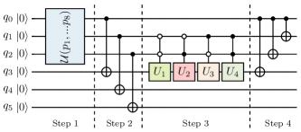
Figure 1: Schematic of the circuit to generate a three-qubit GHZ diagonal PPT mixed state from a six-qubit $|000000\rangle$ state. Step 1 involves applying a unitary operation which is a function of $p_{i}$ values and depends on the state to be prepared. Step 2 consists of CNOT operations. Step 3 involves another unitary operation, also a function of $p_{i}$ values. Step 4 involves additional CNOT operations.

We present a general protocol for creating a 6-qubit pure state similar to the procedure given in Ref. Hyllus et al. (2004):

• Step 1: Begin with an initial three-qubit state $\ket{000}$ and create a pure state of the form:
  $\sqrt{\frac{p_{1}+p_{2}}{2}}(\ket{000}+\ket{100})+\sqrt{\frac{p_{3}+p_{4}}{2}}(\ket{001}+\ket{101})$ $+\sqrt{\frac{p_{5}+p_{6}}{2}}(\ket{010}+\ket{110})+\sqrt{\frac{p_{7}+p_{8}}{2}}(\ket{011}+\ket{111})$

• Step 2: Introduce three ancillary qubits to the system. Apply CNOT gates: CNOT₁₄, CNOT₂₅, CNOT₃₆ (in CNOT_ij, ‘$i$’ denotes the control qubit, and ‘$j$’ signifies the target qubit).

• Step 3: Implement a control unitary operation with qubits 2 and 3 as controls and qubit 4 as the target. The unitary is defined as:

  $$\begin{split}U=&\ket{00}\bra{00}\otimes U_{1}+\ket{01}\bra{01}\otimes U_{2}\\ &+\ket{10}\bra{10}\otimes U_{3}+\ket{11}\bra{11}\otimes U_{4}\end{split}$$ (15)

  $U_{1},U_{2},U_{3},U_{4}$ are given by

  $$U_{k}=\frac{1}{\sqrt{p_{i}+p_{i+1}}}\left(\begin{array}[]{cc}\sqrt{p_{i+1}}&\sqrt{p_{i}}\\ \sqrt{p_{i}}&-\sqrt{p_{i+1}}\\ \end{array}\right)$$

  where, $k=1,2,3,4$ and for $k=1\rightarrow i=1$, $k=2\rightarrow i=5$, $k=3\rightarrow i=7$ and $k=4\rightarrow i=3$.

• Step 4: On applying CNOT₁₂,CNOT₁₃,CNOT₁₄, we get the desired six-qubit pure state. Tracing out qubits 4,5,6 will give the $\rho$ of the form in Eq. 1.

This protocol enables the preparation of the desired six-qubit pure state, using a systematic approach for state generation, which involves ancillary qubits and controlled operations.

A schematic of the protocol is illustrated in Figure 1. The box encompassing qubits 1,2 and 3 represents a unitary operation $\mathcal{U}(p_{1},...p_{8})$ that depends on the values of $p$s. To generate the desired three-qubit pure state from the $\ket{000}$ state, one must determine the values of $p_{1},p_{2},...p_{8}$ that define the state. With this knowledge, generating the state from the initial state becomes straightforward. Using the UniversalQCompiler package, unitary operations involving single and two-qubit gates can be designed to achieve this transformation Iten et al. (2021). The unitaries defined in Step 2 of the protocol are standard two-qubit CNOT operations. To implement the general circuit given in Step 3 on the IBM quantum processor, we decompose it into standard single-qubit gates and CNOT gates using the UniversalQCompiler package. After applying the CNOT operations in Step 4, the first three qubits yield the required state. The expectation values of the witness operators are then measured on these qubits.

IV.2 Experimental Implementation on IBM

In this study, we utilized IBM’s Qiskit framework to execute and optimize quantum computations. We used Qiskit Aer for high-performance simulation on classical hardware, and Qiskit IBM Runtime for efficient execution on IBM’s quantum computers. Our computations were carried out on the IBM Sherbrooke quantum processor (version 1.4.49) featuring a 127-qubit Eagle R3 processor. These experiments aimed to explore this quantum hardware’s potential for detecting entanglement in mixed PPT states.

The IBM Sherbrooke processor uses an advanced architecture that provides higher qubit coherence, resulting in lower gate errors despite longer gate lengths. It has a median Echoed Cross-Resonance (ECR) gate error rate of 7.810e-3, a median single-qubit (SX) gate error rate of 2.164e-4, and a median readout error rate of 1.260e-2. The system offers qubit coherence times, with median T1 and T2 times of 270.58 microseconds and 193.93 microseconds, respectively. Additional performance metrics including readout assignment error, anharmonicity, frequency, and individual gate errors for all qubits, are provided on the IBM website ibm . The spatial arrangement of the 127 qubits on the IBM Sherbrooke processor is depicted in Figure 2, illustrating the qubit connectivity and layout.

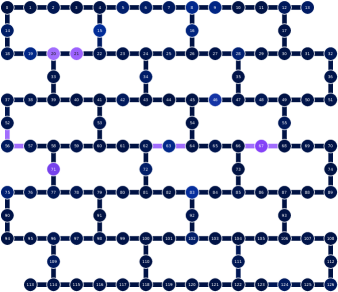
Figure 2: The qubit arrangement in the IBM Sherbrooke processor with 127 qubits.

We set the number of shots (the number of times the quantum circuit was executed) to 10,000. Before executing our quantum circuits on the IBM hardware, we simulated all state circuits and expectation values using the state vector simulator AerSimualtor. These simulations demonstrated excellent agreement with theoretical predictions. This verification step ensured the correctness of our quantum algorithms and helped identify potential issues before running experiments on the physical quantum hardware.

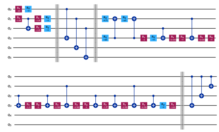
Figure 3: The six-qubit gate sequence with angles and phases of the respective single-qubit gates for the preparation of state 4 on the IBM Sherbrooke system. The vertical lines connecting different qubits represent CNOT gates, with dots indicating control qubits and plus symbols denoting target qubits. Barriers are used to enhance clarity by delineating different sections of the circuit in accordance with the various steps of the protocol.

For our experiments, we employed the EstimatorV2 primitive in IBM Quantum systems, part of Qiskit Runtime, which is designed to efficiently compute the expectation values of quantum operators for parameterized quantum circuits. Various estimator options were configured to optimize the performance of the Estimator methods. To mitigate the effects of decoherence, we enabled dynamical decoupling, a technique that applies a sequence of pulses to refocus the qubits. Additionally, we utilized gate twirling and twirling of measurements to average out errors in quantum gates and measurements, respectively. Measurement error mitigation techniques were also applied to correct for biases in the measurement process.

The Estimator includes methods for error mitigation to improve the accuracy of expectation value computations, crucial for noisy intermediate-scale quantum (NISQ) devices. Error mitigation techniques enable users to reduce circuit errors by modeling the device noise during execution. There are built-in error mitigation techniques in the primitive in the form of resilience options. We explored different resilience levels, which indicate the intensity of error mitigation techniques applied. Resilience level 0 denotes no error mitigation, while resilience levels 1 and 2 involve increasingly advanced techniques to correct errors. Resilience level 2 includes techniques like Zero Noise Extrapolation (ZNE), which estimates results as if there were no noise by running computations at different noise levels and extrapolating back to zero noise. By conducting experiments across these different resilience levels, we were able to assess the effectiveness of various error mitigation strategies and their impact on the accuracy of our quantum computations.

Transpilation is the process of rewriting a given input circuit to match the topology of a specific quantum device, and/or to optimize the circuit for execution on noisy quantum systems. The transpilation process was employed to convert our high-level quantum circuits into a lower-level representation suitable for execution on the IBM Sherbrooke processor. During this process, optimization level 3, the highest level of optimization in Qiskit, was applied to reduce the gate count and circuit depth, thereby improving the fidelity of the quantum computations.

To ensure the reliability of our results, we repeated each experiment three times for each code and each level of resilience, and then calculated the mean and standard deviation of the results. This approach allowed us to quantify the variability and consistency of the measurements under different conditions.

	Theoretical		Experimental Witness
	Witness		Resilience=0		Resilience=1		Resilience=2
State	Linear	Non-Linear	Linear	Non-Linear	Linear	Non-Linear	Linear	Non-Linear
1	-0.2761	-0.6666	-0.0275$\pm$0.0188	-0.5470$\pm$0.0266	-0.0074$\pm$0.0525	-0.5166$\pm$0.0178	-0.2881$\pm$0.0236	-0.6561$\pm$0.0183
2	-0.3314	-0.4000	-0.0580$\pm$0.0223	-0.3068$\pm$0.0249	-0.0371$\pm$0.0925	-0.2977$\pm$0.0317	-0.2124$\pm$0.0665	-0.3491$\pm$0.0270
3	-0.2480	-0.8000	0.3560$\pm$0.0306	-0.3412$\pm$0.0263	0.0849$\pm$0.0229	-0.6356$\pm$0.0322	-0.1238$\pm$0.1045	-0.6906$\pm$0.0957
4	-0.1656	-1.1904	0.1445$\pm$0.0209	-0.8703$\pm$0.0806	0.0674$\pm$0.0373	-0.9669$\pm$0.0231	-0.1495$\pm$0.0666	-1.1916$\pm$0.0786
5	-0.3313	-0.4000	-0.0240$\pm$0.0234	-0.2952$\pm$0.0120	-0.1104$\pm$0.0323	-0.3519$\pm$0.0025	-0.2669$\pm$0.0809	-0.3610$\pm$ 0.0235

Table 1: Comparison of theoretical and experimental witness values for linear and non-linear witnesses under different resilience levels. Experimental results are shown for resilience levels 0, 1, and 2, representing various levels of error mitigation techniques. Each experimental value is the mean $\pm$ standard deviation of the witness values obtained from three experimental runs.

For the Kay state with $a=2$, the numerical values for the expectation values of linear and nonlinear operators are higher. As the value of $a$ increases, these numerical values decrease, especially for the linear witness. This reduction in numerical values diminishes the likelihood of efficient experimental observation. Therefore, we conduct experiments with $a=2$ to maximize the chances of successful and efficient results. During the experimental setup, we designated State 1 as a Kay state with a parameter $a$ set to 2. Applying the same rationale, we opt to use the Kay state with $b=c=2$ for our experimental implementation, referring to it as State 2. As for State 3, State 4, and State 5, they were precisely the states previously described as examples for Category 1, Category 2, and Category 3, respectively.

To generate quantum states, gate sequences were designed based on the approach discussed in the previous subsection, using both the algorithm and the UniversalQCompiler package. An example of such a sequence is depicted in Figure 3, where we illustrate the quantum circuit implemented for State 4 on the IBM Sherbrooke processor.

We conducted experiments on five quantum states by designing circuits as discussed above and using an estimator to determine expectation values, which are essential for calculating both linear and nonlinear quantum witnesses. We utilized estimators with three different resilience levels: 0, 1, and 2. The resilience levels indicate the intensity of error mitigation techniques applied, with higher levels providing more robust error correction. For resilience level 0 (no error mitigation) and 1 which includes basic error mitigation techniques, the IBM Sherbrooke quantum processor took an average of 18-20 seconds to execute the code. For resilience level 2, which incorporates advanced error mitigation techniques like Zero Noise Extrapolation (ZNE), it took 1 minute and 6-10 seconds. This demonstrates that while higher resilience levels improve the accuracy of results, they also require more time to execute. After creating and optimizing (transpiling) the circuits, we executed each code for each state and each resilience level three times. This repetition helped us gather sufficient data to calculate the average behavior and the standard deviation, providing insights into the variability and consistency of the results. The detailed experimental outcomes as well as theoretically expected results for all states are presented in Table 1. Each code execution involved 10,000 shots, ensuring robust statistical data for analysis.

It is noteworthy that while all states exhibited negative values when analyzed using nonlinear witnesses, the linear witnesses failed to detect entanglement in some of the states. We observe that with resilience levels 0 and 1, the results obtained using linear entanglement witnesses are unreliable. However, with resilience level 2, although the results are somewhat reliable, they require longer execution times. On the other hand, nonlinear entanglement witnesses produce reliable results even with resilience level 0. These experiments were conducted under maximum optimization, specifically optimization level 3. This observation underscores the significance of nonlinear entanglement criteria in distinguishing the entangled nature of these states in NISQ devices.

V Conclusion

We examined the entanglement of three-qubit GHZ diagonal bound states by analyzing both linear and nonlinear entanglement witnesses on an IBM quantum processor. The states were prepared by taking three ancilla qubits and expectation values were calculated using the Estimator primitive on IBM runtime. We checked and compared the results of linear and nonlinear witnesses with theoretical expectations using various error mitigation techniques. The presence of entanglement is indicated by negative expectation values of the entanglement witness operators. For all the states prepared on the IBM quantum platform, the nonlinear expectation values were negative, even without error mitigation, providing a strong indication of entanglement. However, the linear expectation values for some states were positive and not very reliable across different resilience levels of error mitigation. This suggests that linear witnesses alone may not be sufficient for reliably detecting entanglement in these cases. This discrepancy highlights the importance of considering nonlinear effects in entanglement analysis. Our findings contribute to a deeper understanding of entanglement detection in near-term quantum computing devices.

References

- Horodecki et al. (2009) R. Horodecki, P. Horodecki, M. Horodecki, and K. Horodecki, Rev. Mod. Phys. 81, 865 (2009).
- Gühne and Tóth (2009) O. Gühne and G. Tóth, Phys. Rep. 474, 1 (2009).
- Das et al. (2016) S. Das, T. Chanda, M. Lewenstein, A. Sanpera, A. Sen De, and U. Sen, Quantum Information (John Wiley & Sons, Ltd, 2016) Chap. 8, pp. 127–174.
- Altepeter et al. (2005) J. B. Altepeter, E. R. Jeffrey, P. G. Kwiat, S. Tanzilli, N. Gisin, and A. Acín, Phys. Rev. Lett. 95, 033601 (2005).
- van Enk et al. (2007) S. J. van Enk, N. Lütkenhaus, and H. J. Kimble, Phys. Rev. A 75, 052318 (2007).
- De Vicente (2007) J. I. De Vicente, Quant. Inf. Comp. 7, 624–638 (2007).
- de Vicente (2008) J. I. de Vicente, J. Phys. A: Math. Ther. 41, 065309 (2008).
- Gühne et al. (2007) O. Gühne, P. Hyllus, O. Gittsovich, and J. Eisert, Phys. Rev. Lett. 99, 130504 (2007).
- Horodecki et al. (1996) M. Horodecki, P. Horodecki, and R. Horodecki, Phys. Lett. A 223, 1 (1996).
- Terhal (2000) B. M. Terhal, Phys. Lett. A 271, 319 (2000).
- Bruß et al. (2002) D. Bruß, J. I. Cirac, P. Horodecki, F. Hulpke, B. Kraus, M. Lewenstein, and A. Sanpera, J. Mod. Optics 49, 1399 (2002).
- Murao and Vedral (2001) M. Murao and V. Vedral, Phys. Rev. Lett. 86, 352 (2001).
- Horodecki et al. (2005) K. Horodecki, M. Horodecki, P. Horodecki, and J. Oppenheim, Phys. Rev. Lett. 94, 160502 (2005).
- Augusiak and Horodecki (2006) R. Augusiak and P. Horodecki, Phys. Rev. A 74, 010305 (2006).
- Smith and Yard (2008) G. Smith and J. Yard, Science 321, 1812 (2008).
- Horodecki et al. (2001) M. Horodecki, P. Horodecki, and R. Horodecki, Phys. Lett. A 283, 1 (2001).
- Terhal (2002) B. M. Terhal, Theor. Comput. Sci. 287, 313 (2002).
- Gühne and Lütkenhaus (2006) O. Gühne and N. Lütkenhaus, Phys. Rev. Lett. 96, 170502 (2006).
- Uffink (2002) J. Uffink, Phys. Rev. Lett. 88, 230406 (2002).
- Gühne (2004) O. Gühne, Phys. Rev. Lett. 92, 117903 (2004).
- Tóth and Gühne (2005) G. Tóth and O. Gühne, Phys. Rev. A 72, 022340 (2005).
- Dür and Cirac (2000) W. Dür and J. I. Cirac, Phys. Rev. A 61, 042314 (2000).
- Gühne and Seevinck (2010) O. Gühne and M. Seevinck, New J. Phys. 12, 053002 (2010).
- Nagata (2009) K. Nagata, Int. J. Theor. Phys. 48, 3358 (2009).
- Aolita et al. (2008) L. Aolita, R. Chaves, D. Cavalcanti, A. Acín, and L. Davidovich, Phys. Rev. Lett. 100, 080501 (2008).
- Kay (2011) A. Kay, Phys. Rev. A 83, 020303 (2011).
- Chen and Jiang (2011) X.-y. Chen and L.-z. Jiang, Phys. Rev. A 83, 052316 (2011).
- Huber et al. (2010) M. Huber, F. Mintert, A. Gabriel, and B. C. Hiesmayr, Phys. Rev. Lett. 104, 210501 (2010).
- Eltschka and Siewert (2012) C. Eltschka and J. Siewert, Phys. Rev. Lett. 108, 020502 (2012).
- Gühne (2011) O. Gühne, Phys. Lett. A 375, 406 (2011).
- García-Pérez et al. (2020) G. García-Pérez, M. A. Rossi, and S. Maniscalco, Npj Quantum Inf. 6, 1 (2020).
- Yeter-Aydeniz et al. (2022) K. Yeter-Aydeniz, S. Bangar, G. Siopsis, and R. C. Pooser, Quant. Inf. Proc. 21, 84 (2022).
- Jha and Chatla (2022) A. K. Jha and A. Chatla, Eur. Phys. J.: Spec. Top. 231, 141 (2022).
- Manabputra et al. (2020) Manabputra, B. K. Behera, and P. K. Panigrahi, Quant. Inf. Proc. 19, 1 (2020).
- Lyu et al. (2021) S. Lyu, K. Wang, Z. Zhang, A. Pedrono, C. Sun, and D. Legendre, J. Comput. Phys. 432, 110160 (2021).
- Tilly et al. (2020) J. Tilly, G. Jones, H. Chen, L. Wossnig, and E. Grant, Phys. Rev. A 102, 062425 (2020).
- Yeter-Aydeniz et al. (2020) K. Yeter-Aydeniz, R. C. Pooser, and G. Siopsis, Npj Quantum Inf. 6, 63 (2020).
- Skosana and Tame (2021) U. Skosana and M. Tame, Sci. Rep. 11, 16599 (2021).
- Amico et al. (2019) M. Amico, Z. H. Saleem, and M. Kumph, Phys. Rev. A 100, 012305 (2019).
- Karimi et al. (2024) N. Karimi, S. N. Elyasi, and M. Yahyavi, Phys. Scr. 99, 045121 (2024).
- Kye (2015) S.-H. Kye, J. Phys. A Math. Theor. 48, 235303 (2015).
- Jafarizadeh et al. (2008) M. A. Jafarizadeh, M. Mahdian, A. Heshmati, and K. Aghayar, Eur. Phys. J. D 50, 107 (2008).
- Weisstein (2002) E. W. Weisstein, CRC concise encyclopedia of mathematics (Chapman and Hall/CRC, 2002).
- Doherty et al. (2005) A. C. Doherty, P. A. Parrilo, and F. M. Spedalieri, Phys. Rev. A 71, 032333 (2005).
- Hyllus et al. (2004) P. Hyllus, C. Moura Alves, D. Bruß, and C. Macchiavello, Phys. Rev. A 70, 032316 (2004).
- Iten et al. (2021) R. Iten, O. Reardon-Smith, E. Malvetti, L. Mondada, G. Pauvert, E. Redmond, R. S. Kohli, and R. Colbeck, “Introduction to universalqcompiler,” (2021), arXiv:1904.01072 [quant-ph] .
- (47) “https://quantum-computing.ibm.com,” .