Probing non-minimal coupling through super-horizon instability and secondary gravitational waves

Abstract

In this paper, we investigate the impact of scalar fluctuations ($\chi$) non-minimally coupled to gravity, $\xi\chi^{2}R$, as a potential source of secondary gravitational waves (SGWs). Our study reveals that when reheating EoS $w_{\phi}>1/3$ and $\xi\gtrsim 1/6$, the super-horizon modes of scalar field experience a Tachyonic instability during the reheating phase. Particularly for $\xi>1$ such instability causes substantial growth in the scalar field amplitude leading to pronounced production of SGWs in an intermediate-frequency range that is strong enough to be detected by future gravitational wave detectors. Such growth in super-horizon modes of the scalar field and associated GW production may have a significant effect on the strength of the tensor fluctuation at the Cosmic Microwave Background (CMB) scales (parametrized by $r$) and the number of relativistic degrees of freedom (parametrized by $\Delta N_{\rm eff}$) at the time of CMB decoupling. To prevent such overproduction, the PLANCK constraints on tensor-to-scalar ratio $r\leq 0.036$ and $\Delta N_{\rm eff}\leq 0.284$ yield a strong upper bound on the value of $\xi$ depending upon the value of $w_{\phi}$ and reheating temperature $T_{\rm re}$. Taking into account all the observational constraints we found the value of $\xi$ should be $\lesssim 4.0$ for any value of reheating temperature within $10^{-2}\lesssim T_{\rm re}\lesssim 10^{14}$ GeV, reheating equation of state within $1/2\leq w_{\phi}\leq 1$, and for a wide range of inflationary energy scales. However, for $w_{\phi}<1/3$, $\xi$ is found to be unconstrained by any known observation. Finally, we identify the parameter regions in $(T_{\rm re},\xi)$ plane which can be probed by the upcoming GW experiments namely BBO, DECIGO, LISA, and ET.

I Introduction

Primordial Gravitational wave (GW) is one of the unique observable predictions of inflationary paradigm Guth (1981); Senatore (2017); Linde (1982); Albrecht and Steinhardt (1982); Lemoine et al. (2008); Mukhanov et al. (1992); Martin (2004, 2005); Linde (2015); Bassett et al. (2006); Sriramkumar (2009); Baumann and Peiris (2009); Baumann (2018); Piattella (2018). Given the advent of a large number of existing Abbott et al. (2016a, b, 2017a, 2017b); Arzoumanian et al. (2020); Agazie et al. (2023a, b); Antoniadis et al. (2023a, b, c); Reardon et al. (2023); Zic et al. (2023); Xu et al. (2023) and upcoming Punturo et al. (2010); Sathyaprakash et al. (2012); Crowder and Cornish (2005); Corbin and Cornish (2006); Baker et al. (2019); Seto et al. (2001); Kawamura et al. (2011); Suemasa et al. (2017); Amaro-Seoane et al. (2013); Barausse et al. (2020); Janssen et al. (2015) GWs detection experiments, inflationary framework proves to be an interesting playground to look for new physics at very high energy scales Arkani-Hamed and Maldacena (2015); Chen and Wang (2010). Exponential expansion leading to tachyonic growth of the super-horizon modes, and their subsequent evolution are known to be imprinted in the distribution of various cosmological relics such as Cosmic Microwave Background (CMB), Dark Matter (DM), GWs in the form of various correlations of scalar, vector and tensor fluctuations. Over the years enormous efforts have been put into estimating those correlations through the CMB anisotropy (Akrami et al. (2020) and references therein), dark and baryonic matter distribution Adame et al. (2024); Ahumada et al. (2020), and placed tight constraints on the possible physics of inflation. Out of those different relics GW is said to be unique due to its extremely weak (Planck suppressed) but universal coupling. Whereas weak coupling renders it an ideal probe of the very early universe, universal coupling on the other enables it to probe into the nature of all fundamental interactions in both the visible and dark sectors. Utilizing inflation as a mechanism, in this paper we intend to probe the non-minimal gravitational coupling $\xi R\chi^{2}$ with a real scalar field $\chi$ through its imprints on the primordial GW spectrum. Such coupling is assumed to be inevitable in the low energy effective theory for the scalar field when coupled with gravity. Non-minimal gravitational coupling has been extensively explored in the context of inflation Faraoni (1996); Tsujikawa (2000); Komatsu and Futamase (1999); Lucchin et al. (1986); Spokoiny (1984); Futamase and Maeda (1989); Shokri et al. (2021); Capozziello and de Ritis (1994); NOZARI and SADATIAN (2008); Gomes et al. (2017); Sarkar et al. (2023), reheating Bassett and Liberati (1998); Tsujikawa et al. (1999a, b); Ema et al. (2017); Dimopoulos and Markkanen (2018); Figueroa et al. (2023); Figueroa and Loayza (2024), DM Markkanen and Nurmi (2017); Markkanen (2018); Fairbairn et al. (2019); Kainulainen et al. (2023); Lebedev et al. (2023); Kolb and Long (2023); Ema et al. (2018); Yu et al. (2023); Kolb and Long (2021); Capanelli et al. (2024a, b), and dark energy Setare and Vagenas (2010); Sami et al. (2012); Kase and Tsujikawa (2020). In the present paper, however, we focus on exploring the dynamics of super Hubble modes and associated induced GW spectrum. This particular aspect of the present study has been less attended to in the literature. Depending on the strength of the non-minimal coupling certain range of super-Hubble modes of the scalar field realize tachyonic growth and may lead to potentially detectable secondary gravitational waves (SGW). Our analysis further reveals that the post-inflationary reheating phase plays an instrumental role. The instability that we pointed out for the super Hubble modes turned out to be significantly strong during the reheating phase, particularly for stiff equation of state $w_{\phi}>1/3$. Such instability leads to stronger scalar field modes growth depending upon the reheating parameters, namely $w_{\phi}$ and reheating temperature $T_{\rm re}$. Further, the cosmological background driven by matter fields with a stiff equation of state is known to amplify GW amplitude when propagating through such background Maiti et al. (2024). In this article, we affirm that a combination of the above two non-trivial effects indeed leads to large GW production. Taking into account CMB constraints on the inflationary tensor power spectrum, and BBN constraints on an effective number of degrees of freedom we demonstrate that SGW induced by non-minimal coupling put a tighter constraint on non-minimal coupling parameters $\xi$ as compared to the values generically assumed in the earlier studies Clery et al. (2022); Barman et al. (2022); Ghoshal et al. (2024) and also constraint recently reported considering primary gravitational waves Maity and Haque (2024). Maintaining all the existing observational constraints we finally estimate the range of non-minimal coupling against different reheating models that can be probed by the various upcoming GW experiments such as BBO, DECIGO, LISA, and ET.

The order of construction of this paper is as follows. In Section II, we first give a brief overview of the non-perturbative framework of gravitational particle production. We then elaborately discuss the super-horizon instability dynamics(Tachyonic instability) of the scalar field in the presence of the non-minimal coupling with gravity $\xi\chi^{2}R$ and we also compute the associated long-wavelength field solutions during reheating corresponding to three different ranges of non-minimal coupling strength, $0\leq\xi<3/16,\xi=3/16,\xi>3/16$ in the entire range of post-inflationary EoS $0\leq w_{\phi}\leq 1$. Further, we thoroughly investigate the behavior of the scalar power spectrum and explicitly point out the salient features of this spectrum for varying parameters ($w_{\phi},~{}\xi$). We close this section by giving a short discussion on the model-independent definition of the reheating parameters ($N_{\rm re},~{}T_{\rm re}$). In Section III, we discuss the dynamics of the tensor fluctuations with (secondary gravitational waves, SGW) and without (primary gravitational waves, PGW) the anisotropy sourced by the gravitationally produced scalar field. In this section, our prime focus is on the effect of the parametric instability being caused by the non-minimal coupling of the scalar field on the gravitational wave spectrum(PGW+SGW). Here we compute the primary as well as the secondary gravitational wave spectrum and show the nature of the full spectrum for varying parameters ($w_{\phi},~{}T_{\rm re},~{}\xi,~{}r_{0.05}$). Furthermore, we constrain the coupling strength $\xi$ in the light of the present-day tensor-to-scalar ratio at the CMB scale $r_{0.05}\leq 0.036$ and the $\Delta N_{\rm eff}\leq 0.284$ bound as reported by the recent PLANCK 2018 observation. We also provide a feasible parameter space of the parameter set ($T_{\rm re},~{}\xi$) that can be detected by future GW detectors like LISA, DECIGO, BBO, ET, etc. Section IV concludes this paper by shedding light on some possible directions of the present work that are left for future endeavors. In Appendix A, we illustrate the computation of the secondary GW spectrum and in Appendix B, we detail the computation of the energy density of the produced scalar field.

II Spectrum of Gravitationally Produced Massless Particles

We shall begin this section by briefly discussing the basic formalism of non-perturbative particle production. We consider the following general Lagrangian for inflaton ($\phi$) and a massive daughter field $(\chi)$ non-minimally coupled to gravity and inflaton as follows.

$$\mathcal{L}_{[\phi,\chi]}=-\sqrt{-g}\bigg{(}\frac{1}{2}\partial_{\mu}\phi\partial^{\mu}\phi+V(\phi)+\frac{1}{2}\partial_{\mu}\chi\partial^{\mu}\chi+\frac{1}{2}(m_{\chi}^{2}+g^{2}\phi^{2}+\xi R)\chi^{2}\bigg{)}.$$ (1)

The background FLRW metric is expressed as $ds^{2}=a^{2}(\eta)\big{(}-d\eta^{2}+d\vec{x}^{2}\big{)}$ with the scale factor $a$ and $\sqrt{-g}=a^{4}(\eta)$. $V(\phi)$ is the inflaton potential, $m_{\chi}^{2}$ is the bare mass of the produced scalar particles. “$\xi$” is the dimensionless non-minimal coupling of $\chi$ field with gravity and $g$ is dimensionless coupling strength with the inflaton. Ricci scalar “$R$” generates a time-dependent effective mass for the $\chi$ field as, $m_{\text{eff}}^{2}(\eta)=\big{(}m_{\chi}^{2}+g^{2}\phi(\eta)^{2}+\xi R(\eta)\big{)}$. Since the background is set by the inflaton which is minimally coupled with gravity, we perform our computation in the Jordon frame for scalar field fluctuation $\chi$.

From the background inflaton part of the Lagrangian (1), we get the inflaton dynamical equation as

$$\phi^{\prime\prime}+2\mathcal{H}\phi^{\prime}+a^{2}\partialderivative{V(\phi)}{\phi}=0.$$ (2)

With the Hubble scale

$$\mathcal{H}=\sqrt{\frac{1}{3M_{pl}^{2}}\bigg{(}\frac{1}{2}(\phi^{\prime})^{2}+a^{2}V(\phi)\bigg{)}},$$ (3)

where $\phi^{\prime}=(d\phi/d\eta)$ and $M_{pl}={1}/{\sqrt{8\pi G}}\approx 2.435\crossproduct 10^{18}\text{Gev}$ is the reduced $Planck$ mass. Different dynamical features of inflaton in the Post-inflationary phase influence the Hubble scale which leaves a non-trivial impact on the particle production process.

Expressing the scalar field “$\chi$” field in terms of Fourier modes,

$$\chi(\eta,{x})=\int\frac{d^{3}{k}}{(2\pi)^{3}}.\chi_{k}(\eta).e^{i{k}\cdot{x}},$$ (4)

and subject to the Lagrangian (1) we reach the following dynamical equation of mode function ($\chi_{{k}})$ as,

$$\chi_{{k}}^{\prime\prime}+2\mathcal{H}\chi_{{k}}^{\prime}+\Big{(}k^{2}+a^{2}(\eta)\big{(}m_{\chi}^{2}+g^{2}\phi^{2}+\xi R\big{)}\Big{)}\chi_{{k}}=0.$$ (5)

In the following dynamical Eq. (5), note that there is a damping term, “$2\mathcal{H}\chi_{{k}}^{\prime}$” which is non-zero in expanding background. Defining a new rescaled field $X_{{k}}=a(\eta)\chi_{{k}}(\eta)$, we obtain the following simplified equation of an oscillator with time-dependent frequency,

$$X_{{k}}^{\prime\prime}+\bigg{[}k^{2}+a^{2}\big{(}m_{\chi}^{2}+g^{2}\phi^{2}\big{)}+\frac{a^{2}R}{6}(6\xi-1)\bigg{]}X_{{k}}=0.$$ (6)

The bracketed term in the above Eq. (6) can be identified as a time-dependent frequency “$\omega_{k}$” where,

$$\omega_{k}^{2}(\eta)=\bigg{(}k^{2}+a^{2}\big{(}m_{\chi}^{2}+g^{2}\phi^{2}\big{)}+\frac{a^{2}R}{6}(6\xi-1)\bigg{)}.$$ (7)

To solve the Eq. (6) we choose the positive frequency Bunch-Davies vacuum,

$$X_{k}(\eta_{0})=\frac{1}{\sqrt{2\omega_{k}}}e^{-i\omega_{k}\eta_{0}},\quad X_{k}^{\prime}(\eta_{0})=-i\sqrt{\frac{\omega_{k}}{2}}e^{-i\omega_{k}\eta_{0}}.$$ (8)

Where $\eta_{0}$ is some initial time at which positive-frequency Bunch-Davies vacuum solution is satisfied. The particle occupation number or number density power spectrum for the scalar field is usually expressed as Kofman et al. (1997),

$$n_{k}=\frac{1}{2\omega_{k}}|\omega_{k}X_{k}-iX_{k}^{\prime}|^{2}.$$ (9)

Integrating Eq.(9) over all the momentum modes, we get the total number and UV convergent energy density as Parker and Fulling (1974); Anderson and Parker (1987)

$$n_{\chi} =\frac{1}{(2\pi)^{3}a^{3}}\int d^{3}kn_{k},$$

$$\rho_{\chi} =\frac{1}{(2\pi)^{3}a^{4}}\int d^{3}k\omega_{k}n_{k}.$$ (10)

The general formalism we constructed in this section is the main foundation of the non-perturbative study of particle production. To this end, we point out that our goal is to analyze the impact of instability due to non-minimal coupling on those modes that remain outside the horizon just after the inflation namely $k<a_{\rm end}H_{\rm end}$. Where $(a_{\rm end},H_{\rm end})$ are the scale factor and Hubble scale at the inflation end respectively. On the other hand, from the expression of the effective frequency $\omega_{k}$ one notes that if the $k\gg a_{\rm end}m_{\chi}$ condition is satisfied, the bare mass of the $\chi$ field can be ignored. Therefore, for the dynamics of the super-horizon modes, the $m_{\chi}\ll H_{\rm end}$ condition is equivalent to the massless limit of the scalar field. This is precisely the limit to which we will perform our computation. We further assume that the $\chi$ field is non-interacting with the standard model and hence it can be assumed as either dark radiation or dark matter. We have checked that as long as the scalar field mass $m_{\chi}\lesssim 10^{-5}H_{\rm end}$, the massless limit is perfectly consistent with our present results. However, the detailed computation for the entire mass range we defer for our future studies.

As just pointed out we consider the massless non-minimally coupled fluctuation which has no other interaction except with gravity. As per these considerations, Lagrangian (1) becomes

$$\mathcal{L}_{[\phi,\chi]}=-\sqrt{-g}\bigg{(}\frac{1}{2}\partial_{\mu}\phi\partial^{\mu}\phi+V(\phi)+\frac{1}{2}\partial_{\mu}\chi\partial^{\mu}\chi+\frac{1}{2}\xi R\chi^{2}\bigg{)}.$$ (11)

The scalar field mode equation (6) becomes,

$$X_{\vec{k}}^{\prime\prime}+\bigg{[}k^{2}-\frac{a^{\prime\prime}}{a}(1-6\xi)\bigg{]}X_{\vec{k}}=0,$$ (12)

where in conformal coordinate, Ricci scalar has been expressed as $R=\left(6a^{\prime\prime}/a^{3}\right)$. In order to calculate the general solution of the above equation (12), we first need to calculate the adibatic vacuum solution of (12) and any general solution of the equation can then be expressed as a linear combination of that vacuum solution with the knowledge of the Bogoliebov coefficients $\alpha_{k}$ and $\beta_{k}$ what we shall compute now.

In the present context, we are interested in the spectrum associated with those modes that left the horizon during inflation and again reenter at some point during reheating and later. These long-wavelength modes experience an instability called Tachyonic instability after getting out of the horizon during inflation. To take into account the enhancement of field amplitude owing to this instability, we study their dynamics from the early inflationary era to the late reheating phase when all the modes are well inside the horizon. The evolution of scale factor during inflation and reheating with any general EoS can be represented as,

$$a(\eta)=\begin{cases}-\frac{1}{H_{\text{end}}\eta}\quad\quad\quad-\infty<\eta\leq\eta_{\text{end}}&\\ a_{\text{end}}\Big{(}\frac{1+3w_{\phi}}{2|\eta_{\rm end}|}\Big{)}^{\frac{2}{1+3w_{\phi}}}\bigg{(}\eta-\eta_{\text{end}}+\frac{2|\eta_{\rm end}|}{1+3w_{\phi}}\bigg{)}^{\frac{2}{1+3w_{\phi}}}\eta\geq\eta_{\text{end}}&\end{cases}.$$ (13)

Considering pure de-Sitter inflation, we assume the Hubble scale at the end of inflation as $H_{\text{end}}$. It is straightforward to check that during the transition from inflation to reheating, the scale factor and its first derivative change continuously at the junction point, that is at the end of inflation, $\eta=\eta_{\text{end}}=-(1/a_{\rm end}H_{\rm end})$. Here $a_{\rm end}$ is the scale factor at $\eta=\eta_{\rm end}$ and $w_{\phi}$ is the background inflaton EoS during reheating.

Associated Hubble scale behaves as

$$\mathcal{H}(\eta\geq\eta_{\rm end})=\frac{a^{\prime}(\eta)}{a(\eta)}=\frac{2(a_{\rm end}H_{\rm end})}{(1+3w_{\phi})}\bigg{(}(\eta a_{\rm end}H_{\rm end})+\frac{3(1+w_{\phi})}{(1+3w_{\phi})}\bigg{)}^{-1}$$ (14)

It is well-known that the violation of the adiabaticity condition owing to the changing background geometry in the abrupt transition from de-Sitter vacuum to post-inflationary vacuum state causes particle production associated with long-wavelength modes. In particular, one defines a dimensionless factor $|\omega^{\prime}_{k}/\omega_{k}^{2}|$ to study the departure from the adiabatic limit and in the process of transition, this adiabaticity condition gets violated($|\omega^{\prime}_{k}/\omega_{k}^{2}|>>1$) at some intermediate point giving a burst of particles in long-wavelength regime.

Now let us suppose $X_{k}^{(\rm inf)}(\eta)$ is the adiabatic vacuum solution of (12) during the de-Sitter phase in the time interval $-\infty<\eta\leq\eta_{\text{end}}$ and $X_{k}^{(\rm reh)}(\eta)$ is the adiabatic vacuum solution during reheating phase for $\eta\geq\eta_{\text{end}}$. Any general field solution during reheating can thus be expressed as

$$X_{k}(\eta)=\alpha_{k}X_{k}^{(\rm reh)}+\beta_{k}X_{k}^{*(\rm reh)},$$ (15)

where, $(\alpha_{k},\beta_{k})$ can be identified as Bogoliubov coefficients. Making these solutions and their first derivatives continuous at the junction $\eta=\eta_{\text{end}}$, we compute the Bogoliubov coefficients as follows: de Garcia Maia (1993)

$$\alpha_{k}=i\left({X_{k}^{(\rm inf)}}^{\prime}(\eta_{\rm end}){X_{k}^{(\rm reh)}}^{*}(\eta_{\rm end})-{X_{k}^{(\rm inf)}}(\eta_{\rm end}){X_{k}^{(\rm reh)}}^{*\prime}(\eta_{\rm end})\right),$$

$$\beta_{k}=-i\left({X_{k}^{(\rm inf)}}^{\prime}(\eta_{\rm end})X_{k}^{(\rm reh)}(\eta_{\rm end})-{X_{k}^{(\rm reh)}}^{\prime}(\eta_{\rm end})X_{k}^{(\rm inf)}(\eta_{\rm end})\right),$$ (16)

where (^′) denotes the derivative with respect to conformal time.

Now, our goal would be to obtain the adiabatic vacuum solutions in both the phases. Using the scale factor (13) in the equation (12), we obtain the form of the dynamical equation during de-Sitter inflation ($\eta\leq\eta_{\text{end}}$) as,

$$X_{k}^{\prime\prime}+\underbrace{\Bigg{[}k^{2}-\frac{2(1-6\xi)}{\eta^{2}}\Bigg{]}}_{\omega_{k}^{2}}X_{k}=0.$$ (17)

From the above equation it can be noted that long wavelength modes after their horizon crossing becomes tachyonic ($\omega_{k}^{2}<0$) for $0\leq\xi<1/6$. As $\xi$ exceeds the conformal limit $\xi=1/6$, this instability ceases to exist.

The general solution of this equation is

$$X_{k}=C_{1}\sqrt{|\eta|}J_{\nu_{1}}(k|\eta|)+C_{2}\sqrt{|\eta|}Y_{\nu_{1}}(k|\eta|).$$ (18)

With the order of the Bessel functions $\nu_{1}={\sqrt{9-48\xi}}/{2}$ and $C_{1},C_{2}$ are integration constants. To evaluate $\alpha_{k}$ and $\beta_{k}$, we need to define first the vacuum solution $X_{k}^{(\rm inf)}$ during inflation. To compute the de-Sitter vacuum solution, we use the Bunch-Davies vacuum condition at the beginning of inflation. In this limit $k|\eta|>>1$, the mode solution (18) becomes,

$$X_{k}(\eta)\sim\frac{1}{\sqrt{2\pi k}}\bigg{[}(C_{1}-iC_{2})e^{-i(k\eta+\pi/4+\pi\nu_{1}/2)}+(C_{1}+iC_{2})e^{i(k\eta+\pi/4+\pi\nu_{1}/2)}\bigg{]}.$$ (19)

In the asymptotic in-vacuum limit, the positive-frequency outgoing mode function behaves as

$$X_{k}(\eta)\xrightarrow{{\eta}\rightarrow-\infty}\frac{e^{-ik\eta}}{\sqrt{2k}}.$$ (20)

Comparing (19) with (20) we have

$$C_{1}=\frac{\sqrt{\pi}}{2}e^{i(\pi/4+\pi\nu_{1}/2)},\quad C_{2}=\frac{i\sqrt{\pi}}{2}e^{i(\pi/4+\pi\nu_{1}/2)}.$$ (21)

Therefore, the adiabatic vacuum solution during de-Sitter inflation is

$$X_{k}^{(\rm inf)}=\frac{\sqrt{-\pi\eta}}{2}e^{i(\pi/4+\pi\nu_{1}/2)}H^{(1)}_{\nu_{1}}(-k\eta).$$ (22)

Similarly the dynamical equation for general post-inflationary($\eta>\eta_{\rm end}$) EoS “$w_{\phi}$” is

$$X_{k}^{\prime\prime}+\underbrace{\Bigg{[}k^{2}-\frac{2(1-3w_{\phi})(1-6\xi)}{(1+3w_{\phi})^{2}\Big{(}\eta+\frac{3(1+w_{\phi})}{a_{\rm end}H_{\text{end}}(1+3w_{\phi})}\Big{)}^{2}}\Bigg{]}}_{\omega_{k}^{2}}X_{k}=0,$$ (23)

From the above equation, it can be again noted that the modes which were stable during inflation for $\xi>1/6$ become tachyonic ($\omega_{k}^{2}<0$) during reheating for $w_{\phi}>1/3$ Fairbairn et al. (2019). We will see that this will play a significant role in our subsequent studies. The general solution of this equation is

$$X_{k}(\eta)=C_{3}4^{\nu_{2}}\Gamma(\nu_{2}+1)\sqrt{2ik\bar{\eta}}I_{\nu_{2}}(ik\bar{\eta})+C_{4}\sqrt{\frac{2ik\bar{\eta}}{\pi}}K_{\nu_{2}}(ik\bar{\eta}).$$ (24)

Where we use the symbol $\bar{\eta}=(\eta+{3\mu}/a_{\rm end}H_{\text{end}})$. $I_{\nu_{2}}$ and $K_{\nu_{2}}$ are modified Bessel functions of order $\nu_{2}$ with

$$\mu=\frac{(1+w_{\phi})}{(1+3w_{\phi})},\quad\nu_{2}=\frac{\sqrt{3(1+w_{\phi})\Big{(}3(1-w_{\phi})^{2}+16\xi(3w_{\phi}-1)\Big{)}}}{2\sqrt{1+3w_{\phi}}\sqrt{1+4w_{\phi}+3w_{\phi}^{2}}}.$$ (25)

and $C_{3},C_{4}$ are the integration constants.

We now seek the solution of (23) compatible with the requirements of an adiabatic vacuum. If spacetime changes very slowly or equivalently particle momentum is so large that it hardly feels the background dynamics, the mode function can be safely assumed to behave as a positive frequency mode in Minkowski space in its asymptotic limit. For this we assume the ($k\eta>>1$) limit, and the mode solution (24) transforms into,

$$X_{k}(\eta)\sim\Bigg{[}C_{3}\frac{2^{2\nu_{2}}\Gamma(\nu_{2}+1)}{\sqrt{\pi}}e^{ik\bar{\eta}}+C_{4}e^{-ik\bar{\eta}}\Bigg{]}.$$ (26)

In the adiabatic out-vacuum limit that is for $\eta>>1$ or equivalently $a(\eta)\rightarrow\infty$ mode function behaves as a positive frequency state

$$X_{k}(\eta)\xrightarrow{{\eta}\rightarrow\infty}\frac{e^{-ik\eta}}{\sqrt{2k}},$$ (27)

Comparing (26) with (27) we have

$$C_{3}=0,\quad C_{4}=\frac{1}{\sqrt{2k}}\text{exp}\bigg{[}\frac{3ik\mu}{a_{\rm end}H_{\text{end}}}\bigg{]}.$$ (28)

Therefore, the adiabatic vacuum solution of massless particles for general reheating EoS “$w_{\rm re}$” becomes

$$X_{k}^{(\rm reh)}(\eta)=\sqrt{\frac{\bar{\eta}}{\pi}}\text{exp}\bigg{[}\frac{3ik\mu}{a_{\rm end}H_{\text{end}}}+\frac{i\pi}{4}\bigg{]}K_{\nu_{2}}(ik\bar{\eta}).$$ (29)

It is important to note that depending upon the value of the non-minimal coupling constant $\xi$, the order of the inflationary vacuum solution $\nu_{1}$ becomes positive for $0\leq\xi<3/16$, zero for $\xi=3/16$, and imaginary for $\xi>3/16$. In addition to this, the index of post-inflationary vacuum solution $\nu_{2}$ also becomes imaginary in the range $\xi>3/16$ for EoS $0\leq w_{\phi}<1/3$ and it becomes real positive for $1/3\leq w_{\phi}\leq 1$. This varying nature of the indices $\nu_{1},\nu_{2}$ depending upon different ranges of non-minimal coupling strength and post-inflationary EoS greatly influences the nature of the post-inflationary field solution. Now we shall compute the field solution during reheating for general EoS in three specified ranges of the non-minimal coupling strength $\xi$.

II.1 Large scale massless field solution for $0\leq w_{\phi}<1/3$

II.1.1 For $0\leq\xi<3/16$ :

As mentioned earlier, the general field solution in a particular phase can be expressed as a linear combination of the respective vacuum solution with the help of Bogoliubov coefficients $\alpha_{k}$ and $\beta_{k}$ (See Eq.(15). So, our main task is to compute $\alpha_{k}$ and $\beta_{k}$ using the relations in (II). In this specified range of $\xi$ we get both $\nu_{1}$ and $\nu_{2}$ to be positive definite. Substituting these vacuum solutions (22) and (29) into (II), in long-wavelength limit $k/k_{\rm end}<<1$, we compute the Bogoliubov coefficients as

$$\alpha_{k}\approx\frac{\Gamma(\nu_{1})\Gamma(\nu_{2})2^{\nu_{1}}}{8\pi}\left(\frac{2}{3\mu-1}\right)^{\nu_{2}}\left(\frac{3\mu(1-2\nu_{1})+2(\nu_{1}-\nu_{2})}{\sqrt{(3\mu-1)}}\right)\left(\frac{1}{\bar{k}}\right)^{\nu_{1}+\nu_{2}}e^{i\left(\frac{\pi\nu_{1}}{2}+\frac{\pi\nu_{2}}{2}+\frac{\pi}{2}-3\mu\bar{k}\right)}$$

$$\beta_{k}\approx\alpha_{k}e^{i\left(-\pi\nu_{2}-\frac{\pi}{2}+6\mu\bar{k}\right)}$$ (30a)

For simplified expression we define a new symbol $\bar{k}=k/k_{\rm end}$. We define the energy density of the produced particles at a time during reheating when the associated longest wavelength is well inside the horizon. In this sense, we always have $k\eta>>1$ for any mode which will contribute to the energy density. Using the long-wavelength approximated form of the coefficients $\alpha_{k}$ and $\beta_{k}$(See Eq.(30)) in (15) we obtain the general long-wavelength solution of scalar field for general EoS in the specified $\xi$ range for $k\eta>>1$ as

$$X^{\rm long}_{k}(\eta)\approx\frac{\Gamma(\nu_{1})\Gamma(\nu_{2})2^{\nu_{1}}}{4\pi\sqrt{k_{\rm end}}}\left(\frac{2}{3\mu-1}\right)^{\nu_{2}}\left(\frac{3\mu(1-2\nu_{1})+2(\nu_{1}-\nu_{2})}{\sqrt{2(3\mu-1)}}\right)\frac{\text{cos}(k\eta)}{\bar{k}^{(\nu_{1}+\nu_{2}+1/2)}}$$ (31)

where $k_{\rm end}=a_{\rm end}H_{\rm end}$ is the scale that leaves the horizon at the end of inflation.

II.1.2 For $\xi=3/16$ :

For this particular value of the coupling strength $\xi$, $\nu_{1}$ vanishes. Following the same procedure, in the long-wavelength limit, $\alpha_{k}$ and $\beta_{k}$ can now be evaluated as

$$\alpha_{k}\approx-\frac{\Gamma(\nu_{2})}{2}\left(\frac{2}{3\mu-1}\right)^{\nu_{2}}\left(\frac{3\mu-2\nu_{2}}{4\sqrt{(3\mu-1)}}+\frac{i\sqrt{3\mu-1}}{\pi}\right)\frac{{\rm exp}\left(i(\pi\nu_{2}/2-\pi/2-3\mu\bar{k})\right)}{\bar{k}^{\nu_{2}}}$$ (32a)

$$\beta_{k}\approx\frac{\Gamma(\nu_{2})}{2}\left(\frac{2}{3\mu-1}\right)^{\nu_{2}}\left(\frac{3\mu-2\nu_{2}}{4\sqrt{(3\mu-1)}}+\frac{i\sqrt{3\mu-1}}{\pi}\right)\frac{{\rm exp}\left(i(-\pi\nu_{2}/2+3\mu\bar{k})\right)}{\bar{k}^{\nu_{2}}}$$ (32b)

Associated general field solution for $\xi=3/16$ in $k\eta>>1$ limit becomes

$$X^{\rm long}_{k}(\eta)\approx\frac{\Gamma(\nu_{2})}{\sqrt{2k_{\rm end}}}\left(\frac{2}{3\mu-1}\right)^{\nu_{2}}\left(\frac{3\mu-2\nu_{2}}{4\sqrt{(3\mu-1)}}+\frac{i\sqrt{3\mu-1}}{\pi}\right)\frac{i\text{sin}(k\eta)}{\bar{k}^{\nu_{2}+1/2}}$$ (33)

II.1.3 For $\xi>3/16$ :

In this range of $\xi$ values, $\nu_{1}$ and $\nu_{2}$ become imaginary. Long-wavelength approximated Bogolieubov coefficients are

$$\alpha_{k}\approx \bigg{(}K_{\nu_{2}}\Big{(}i\bar{k}(3\mu-1)\Big{)}H^{(1)}_{\nu_{1}}(\bar{k})\left(\frac{3\mu}{\sqrt{3\mu-1}}\right)+\bar{k}\sqrt{3\mu-1}\Big{(}H^{(1)}_{\nu_{1}-1}(\bar{k})-H^{(1)}_{\nu_{1}+1}(\bar{k})\Big{)}\bigg{)}$$

$$\begin{split}&\times\text{exp}(i(\pi/2)-3\mu\bar{k})\frac{\text{exp}(-\pi\tilde{\nu}_{1}/2)}{4}\end{split}$$ (34a)

$$\beta_{k}\approx \bigg{(}K_{\nu_{2}}\Big{(}i\bar{k}(3\mu-1)\Big{)}H^{(1)}_{\nu_{1}}(\bar{k})\left(\frac{3\mu}{\sqrt{3\mu-1}}\right)+\bar{k}\sqrt{3\mu-1}\Big{(}H^{(1)}_{\nu_{1}-1}(\bar{k})-H^{(1)}_{\nu_{1}+1}(\bar{k})\Big{)}\bigg{)}$$

$$\begin{split}&\times\text{exp}(3\mu\bar{k})\frac{\text{exp}(-\pi\tilde{\nu}_{1}/2)}{4}\end{split}$$ (34b)

General field solution for $\xi>3/16$ becomes

$$X^{\rm long}_{k}(\eta)\approx \frac{\text{exp}(-\pi\tilde{\nu}_{1}/2)}{4\sqrt{2k_{\rm end}}}\bigg{(}K_{\nu_{2}}\Big{(}i\bar{k}(3\mu-1)\Big{)}H^{(1)}_{\nu_{1}}(\bar{k})\left(\frac{3\mu}{\sqrt{3\mu-1}}\right)+\bar{k}\sqrt{3\mu-1}$$

$$\times\Big{(}H^{(1)}_{\nu_{1}-1}(\bar{k})-H^{(1)}_{\nu_{1}+1}(\bar{k})\Big{)}\bigg{)}\frac{\text{cos}(k\eta)}{\bar{k}^{1/2}}$$ (35)

where $\tilde{\nu}_{1}=(\sqrt{48\xi-9})/2$.

II.2 Large scale Massless field solution for $1/3\leq w_{\phi}\leq 1$

II.2.1 For $0\leq\xi<3/16$ :

Likewise in the previous case, the indices $\nu_{1},\nu_{2}$ are also real positive in this EoS range. In the limit $k/k_{\rm end}<<1$, using equations (22),(29), and (II), we obtain Bogoliebov coefficients as

$$\alpha_{k}\approx-\frac{\Gamma(\nu_{1})\Gamma(\nu_{2})2^{\nu_{1}}}{8\pi}\left(\frac{2}{3\mu-1}\right)^{\nu_{2}}\left(\frac{3\mu(1-2\nu_{1})+2(\nu_{1}-\nu_{2})}{\sqrt{(3\mu-1)}}\right)\frac{{\rm exp}\left(i(\pi\nu_{1}/2+\pi\nu_{2}/2-\pi/2-3\mu\bar{k})\right)}{\bar{k}^{(\nu_{1}+\nu_{2})}}$$ (36a)

$$\beta_{k}\approx\frac{\Gamma(\nu_{1})\Gamma(\nu_{2})2^{\nu_{1}}}{8\pi}\left(\frac{2}{3\mu-1}\right)^{\nu_{2}}\left(\frac{3\mu(1-2\nu_{1})+2(\nu_{1}-\nu_{2})}{\sqrt{(3\mu-1)}}\right)\frac{{\rm exp}\left(i(\pi\nu_{1}/2-\pi\nu_{2}/2+3\mu\bar{k})\right)}{\bar{k}^{(\nu_{1}+\nu_{2})}}$$ (36b)

Subject to the following coefficients, the general field solution in $k\eta>>1$ limit becomes

$$X^{\rm long}_{k}(\eta)\approx\frac{\Gamma(\nu_{1})\Gamma(\nu_{2})2^{\nu_{1}}}{4\pi\sqrt{k_{\rm end}}}\left(\frac{2}{3\mu-1}\right)^{\nu_{2}}\left(\frac{3\mu(1-2\nu_{1})+2(\nu_{1}-\nu_{2})}{\sqrt{2(3\mu-1)}}\right)\frac{i\text{sin}(k\eta)}{\bar{k}^{(\nu_{1}+\nu_{2}+1/2)}}$$ (37)

II.2.2 For $\xi=3/16$ :

For this particular value of $\xi$, the expression of Bogoliebov coefficients as well as general field solution will remain same for this EoS range $1/3\leq w_{\phi}\leq 1$ also. Here also we obtain $\alpha_{k}$ and $\beta_{k}$ as

$$\alpha_{k}\approx-\frac{\Gamma(\nu_{2})}{2}\left(\frac{2}{3\mu-1}\right)^{\nu_{2}}\left(\frac{3\mu-2\nu_{2}}{4\sqrt{(3\mu-1)}}+\frac{i\sqrt{3\mu-1}}{\pi}\right)\frac{{\rm exp}\left(i(\pi\nu_{2}/2-\pi/2-3\mu\bar{k})\right)}{\bar{k}^{\nu_{2}}}$$ (38a)

$$\beta_{k}\approx\frac{\Gamma(\nu_{2})}{2}\left(\frac{2}{3\mu-1}\right)^{\nu_{2}}\left(\frac{3\mu-2\nu_{2}}{4\sqrt{(3\mu-1)}}+\frac{i\sqrt{3\mu-1}}{\pi}\right)\frac{{\rm exp}\left(i(-\pi\nu_{2}/2+3\mu\bar{k})\right)}{\bar{k}^{\nu_{2}}}$$ (38b)

Associated general field solution for $\xi=3/16$ in $k\eta>>1$ limit will be

$$X^{\rm long}_{k}(\eta)\approx\frac{\Gamma(\nu_{2})}{\sqrt{2k_{\rm end}}}\left(\frac{2}{3\mu-1}\right)^{\nu_{2}}\left(\frac{3\mu-2\nu_{2}}{4\sqrt{(3\mu-1)}}+\frac{i\sqrt{3\mu-1}}{\pi}\right)\frac{i\text{sin}(k\eta)}{\bar{k}^{\nu_{2}+1/2}}$$ (39)

II.2.3 For $\xi>3/16$ :

A significant difference in terms of spectral behavior will appear between two given EoS ranges in this particular case $\xi>3/16$. In this case, we get one index $\nu_{1}$ to be imaginary as expected but another index $\nu_{2}$ to be real positive which differs from the previous case for $0\leq w_{\phi}<1/3$. This causes a noticeable change in the spectral behavior as we see soon. Long-wavelength approximated coefficients are evaluated to be

$$\alpha_{k}\approx \frac{\Gamma(\nu_{2})\text{exp}(-\pi\tilde{\nu}_{1}/2)}{8}\left(\frac{3\mu-2\nu_{2}}{\sqrt{(3\mu-1)}}H^{(1)}_{\nu_{1}}(\bar{k})+\bar{k}\sqrt{3\mu-1}\Big{(}H^{(1)}_{\nu_{1}-1}(\bar{k})-H^{(1)}_{\nu_{1}+1}(\bar{k})\Big{)}\right)$$

$$\times\frac{{\rm exp}\left(i(\pi\nu_{2}/2+\pi/2-3\mu\bar{k})\right)}{\bar{k}^{\nu_{2}}}\left(\frac{2}{3\mu-1}\right)^{\nu_{2}}$$ (40a)

$$\beta_{k}\approx \frac{\Gamma(\nu_{2})\text{exp}(-\pi\tilde{\nu}_{1}/2)}{8}\left(\frac{3\mu-2\nu_{2}}{\sqrt{(3\mu-1)}}H^{(1)}_{\nu_{1}}(\bar{k})+\bar{k}\sqrt{3\mu-1}\Big{(}H^{(1)}_{\nu_{1}-1}(\bar{k})-H^{(1)}_{\nu_{1}+1}(\bar{k})\Big{)}\right)$$

$$\times\frac{{\rm exp}\left(i(3\mu\bar{k}-\pi\nu_{2}/2)\right)}{\bar{k}^{\nu_{2}}}\left(\frac{2}{3\mu-1}\right)^{\nu_{2}}$$ (40b)

Therefore, the associated general field solution takes the following form.

$$X^{\rm long}_{k}(\eta)\approx \frac{\Gamma(\nu_{2})\text{exp}(-\pi\tilde{\nu}_{1}/2)}{4\sqrt{2k_{\rm end}}}\left(\frac{3\mu-2\nu_{2}}{\sqrt{(3\mu-1)}}H^{(1)}_{\nu_{1}}(\bar{k})+\bar{k}\sqrt{3\mu-1}\Big{(}H^{(1)}_{\nu_{1}-1}(\bar{k})-H^{(1)}_{\nu_{1}+1}(\bar{k})\Big{)}\right)$$

$$\times\frac{\text{cos}(k\eta)}{\bar{k}^{\nu_{2}+1/2}}\left(\frac{2}{3\mu-1}\right)^{\nu_{2}}$$ (41)

From our analysis so far it is revealed that the long-wavelength scalar field modes gets amplified through tachyonic instability during and after inflation depending upon the value of $(\xi,w_{\phi})$. To this end let us reiterate again that for $0\leq\xi<1/6$ long wavelength modes after their horizon crossing during inflation, get amplified due to tachyonic instability effect (see Eq.(17)). As $\xi$ exceeds the conformal limit $\xi=1/6$, the inflationary instability diminishes, whereas new tachyonic instability develops during reheating, particularly for stiff equation of state $w_{\phi}>1/3$ (see Eq.(23). Enhancement of the scalar field modes due to those instabilities can indeed be observed in Fig.1. In the figure we have plotted the time evolution of different field modes assuming $\xi=3$ for three different equations of state $w_{\phi}=(0,1/3,1/2)$. It can indeed be seen that for $\xi>1/6,w_{\phi}>1/3$, the amplitude of the field modes increases appreciably.

Clearly, the excitation of these large-scale modes owing to the instability effect during inflation for $0\leq\xi<1/6$) and after the inflation for $\xi>1/6$ and $w_{\phi}>1/3$ motivates us to investigate the induced GWs. In the subsequent study of the generation of secondary GWs sourced by the anisotropy, we pay attention to the long-wavelength modes of the source , that lie in the range $k_{\rm re}<k<k_{\rm end}$ where $k_{\rm re}=a_{\rm re}H_{\rm re}$ is the mode which enters the Hubble horizon at the end of reheating.

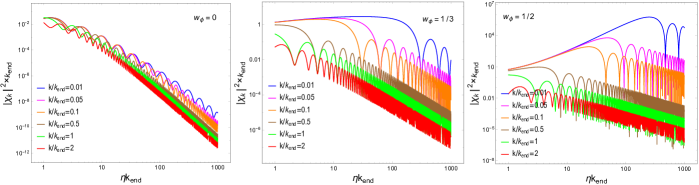
Figure 1: Figure represents the time-evolution of dimensionless field amplitude square $(|\chi_{k}|^{2}\times k_{\rm end})$ associated with some large scale($k<k_{\rm end}$) and small scale($k>k_{\rm end}$) modes for three different EoS. In all three plots, we choose the non-minimal coupling strength to be $\xi=3$. It is clearly seen that for $\xi>1/6$, the post-inflationary instability effect associated with long-wavelength modes is effective for $w_{\phi}>1/3$ as discussed earlier.

II.3 Behavior of scalar power spectrum $\mathcal{P}_{\chi}(k,\eta)$

While defining the anisotropic stress tensor later, we require the nature of the power spectrum of the source field rather than the comoving number density spectrum. Here we define the power spectrum of long-wavelength massless fluctuations corresponding to the original field mode $\chi_{k}$ in the entire post-inflationary EoS range $0\leq w_{\phi}\leq 1$ for three different $\xi$ ranges as follows.

II.3.1 For $0\leq w_{\phi}<1/3$ :

$$\mathcal{P}_{\chi}(k,\eta>\eta_{\rm end})=\frac{k^{3}}{2\pi^{2}}|\chi^{\rm long}_{k}|^{2}\propto\begin{cases}(\text{cos}^{2}(k\eta)/a(\eta)^{2})(k/k_{\rm end})^{2(1-\nu_{1}-\nu_{2})}&\text{for}\quad 0\leq\xi<3/16\\ (\text{sin}^{2}(k\eta)/a(\eta)^{2})(k/k_{\rm end})^{2(1-\nu_{2})}&\text{for}\quad\xi=3/16\\ (1/a(\eta)^{2})(k/k_{\rm end})^{2}&\text{for}\quad\xi>3/16\end{cases}$$ (42)

II.3.2 For $1/3\leq w_{\phi}\leq 1$ :

$$\mathcal{P}_{\chi}(k,\eta>\eta_{\rm end})=\frac{k^{3}}{2\pi^{2}}|\chi^{\rm long}_{k}|^{2}\propto\begin{cases}(\text{sin}^{2}(k\eta)/a(\eta)^{2})(k/k_{\rm end})^{2(1-\nu_{1}-\nu_{2})}&\text{for}\quad 0\leq\xi<3/16\\ (\text{sin}^{2}(k\eta)/a(\eta)^{2})(k/k_{\rm end})^{2(1-\nu_{2})}&\text{for}\quad\xi=3/16\\ (\text{cos}^{2}(k\eta)/a(\eta)^{2})(k/k_{\rm end})^{2(1-\nu_{2})}&\text{for}\quad\xi>3/16\end{cases}$$ (43)

Depending upon EoS in three ranges $0\leq w_{\phi}<1/3$, $w_{\phi}=1/3$, and $1/3\leq w_{\phi}\leq 1$, the scalar power spectrum $\mathcal{P}_{\chi}(k,\eta)$ has interesting spectral behavior with the variation of coupling strength $\xi$. We first illustrate those important features of the power spectrum at a fixed time(and this is true for any time) for varying EoS $w_{\phi}$ in different ranges of $\xi$ values. We shall next discuss the behavior of the spectrum at varying instants of time for a fixed coupling strength.

II.3.3 Spectral behavior at a fixed time :

We study the nature of the power spectrum for varying coupling strength at a fixed time during reheating.

• For $0\leq w_{\phi}<1/3$ :   Examining the spectrum as given in (42) for $0\leq w_{\phi}<1/3$, we find that for $0\leq\xi<1/6$, the spectrum is red-tilted $\mathcal{P}_{\chi}(k,\eta)\propto k^{2(1-\nu_{1}-\nu_{2})}$ with $(1-\nu_{1}-\nu_{2})<0$. However, the amount of red tilt depends upon the choice of EoS $w_{\phi}$ through the following relations,

  $$\nu_{1}=\frac{\sqrt{9-48\xi}}{2}~{}~{}~{};~{}~{}~{}\nu_{2}=\frac{\sqrt{3(1+w_{\phi})\Big{(}3(1-w_{\phi})^{2}+16\xi(3w_{\phi}-1)\Big{)}}}{2\sqrt{1+3w_{\phi}}\sqrt{1+4w_{\phi}+3w_{\phi}^{2}}}.$$ (44)

  With the above mentioned parameter ranges $\nu_{2}$ should lie within $\sqrt{9-48\xi}/2>\nu_{2}>1/2$. For example, as $w_{\phi}$ approaches zero the spectrum becomes maximally red-tilted $\mathcal{P}_{\chi}(k,\eta)\propto k^{(1-2\nu_{1})}$ for given $\xi<1/6$ up to the sinusoidal function of $k$. Such red tilt can indeed be observed in the blue curve in the left panel of Fig. 2. Once $\xi$ exceeds conformal limit $\xi>1/6$, the spectrum turns blue-tilted till one reaches the $\xi=3/16$. As $\xi$ exceeds 3/16, both the indices $\nu_{1},\nu_{2}$ being imaginary results in the power spectrum being insensitive to the non-minimal coupling strength with $\mathcal{P}_{\chi}(k,\eta)\propto k^{2}$. In the left panel of Fig. 2 we can indeed see the blue titled spectrum for $\xi=(0.18,3/16,1,4)$ in magenta, brown, green and red respectively. In summary, in the entire range of $\xi>1/6$, the spectrum being blue-tilted draws the maximum contribution to the amplitude of the scalar power spectrum amplitude for those modes which left the horizon at the inflation end, that is $k_{\rm end}$.

• For $w_{\phi}=1/3$ :   For this particular value of the equation of state, $\nu_{2}=1/2$ irrespective of the choice of $\xi$, and in the range $0\leq\xi<1/6$, $\nu_{1}$ lies within $[3/2,1/2)$. Consequently, in the range $0\leq\xi<1/6$, the scalar spectrum becomes red-tilted as shown in the blue color in the middle panel of Fig. 2 (for $\xi=0$). As $\xi$ exceeds the conformal limit, the index $\nu_{1}$ gradually decreases with the increase of $\xi$ up to $\xi=3/16$, and in this range, $\nu_{1}$ lies within $(0.5,0]$. According to the spectral index given in Eq.(43), spectrum in the range $1/6<\xi\leq 3/16$ becomes blue-tilted as shown in magenta and brown color for $\xi=(0.18,3/16)$ respectively in the middle panel of Fig. 2. For $\xi>3/16$, $\nu_{1}$ becomes imaginary as is obvious from (44). With the further increase of $\xi$, the independence of $\nu_{2}$ makes the slope of the spectrum completely insensitive to the coupling strength in the entire range $\xi>3/16$ although our numerical analysis shows very slow growth of the amplitude wit increasing $\xi$. From the spectral index given in Eq.(43), in the range $\xi\geq 3/16$, the power spectrum behaves as $\mathcal{P}_{\chi}(k,\eta)\propto k$.

• For $1/3<w_{\phi}\leq 1$ :   In the range $0\leq\xi<1/6$, again we obtain a red-tilted power spectrum, and as $\xi$ exceeds the conformal limit, the spectrum turns out to be blue-tilted and it remains so up to $\xi=3/16$ like the previous two cases. However, for $\xi>3/16$, the power spectrum has some noticeable features. For this case $\nu_{2}$ should lie within the range $(1/2,\sqrt{3\xi/2})$. Given an EoS $w_{\phi}>1/3$, there exists a particular coupling strength say, $\xi_{\rm cri}=\frac{(3w_{\phi}+5)(9w_{\phi}-1)}{48(3w_{\phi}-1)}$, at which the spectrum becomes perfectly scale-invariant giving $(1-\nu_{2})=0$ (see Eq.(43)). For $3/16<\xi<\xi_{\rm cri}$, energy spectrum remains blue-tilted, $(1-\nu_{2})>0$. As coupling exceeds the critical value $\xi_{\rm cri}$, the spectrum departs from blue-tilted behavior and becomes red-tilted, $(1-\nu_{2})<0$.

  All these important characteristics of the power spectrum are shown in Fig.2 for three EoS $w_{\phi}=0,w_{\phi}=1/3,\text{and}~{}w_{\phi}=0.5$ for different $\xi$ values at some point of time during reheating. Variations of spectral tilt with the variation of $\xi$ are believed to leave a discernible imprint on the induced GWs spectrum, which we intend to investigate in the subsequent section.

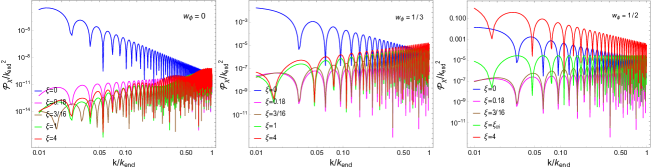
Figure 2: Figure represents the variation of power spectrum $\mathcal{P}_{\chi}(k,\eta)/k_{\rm end}^{2}$ with non-minimal coupling strength $\xi$ for three reheating EoS, $w_{\phi}=0,~{}1/3,~{}1/2$. For $w_{\phi}=1/2$, the critical coupling $\xi_{\rm cri}\approx 0.95$.

II.3.4 Spectral behavior for varying time :

Here we show for a certain coupling strength how the spectral shape will change over time during the reheating phase. We notice that as we go deep into the reheating phase $\eta>>\eta_{\rm end}$, amplitude of the spectrum gets diminished for a given $k$-mode as obvious in Fig.3, and this is because of the decaying nature of every mode after horizon reentry during reheating. For the chosen value of coupling strength $\xi=3$, the blue-tilted( for $w_{\phi}=0,1/3$ ), and red-tilted( for $w_{\phi}=0.5$) nature of the spectrum are also consistent with the expressions given in Eqs. (42) and (43).

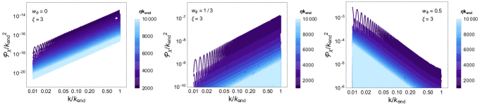
Figure 3: Figure represents the behavior of power spectrum $\mathcal{P}_{\chi}(k,\eta)/k_{\rm end}^{2}$ for three EoS and a specific coupling strength $\xi=3$ with the variation of dimensionless time-variable $\eta k_{\rm end}$ indicated by the color bar where the color gradient is indicating this time-evolution in the post-inflationary phase.

II.4 Defining the Reheating Parameters ($N_{\rm re}$, $T_{\rm re}$) :

In this section we introduce pivotal inflationary parameters namely the inflationary energy scale ($H_{\rm end}$), the duration of the inflationary period denoted by e-folding number $N_{\ast}$, and define a crucial reheating parameter, namely the Reheating Temperature ($T_{\rm re}$). From the CMB pivot scale, we have $(k_{\ast}/a_{0})=0.05\mathrm{Mpc}^{-1}$ where $a_{0}$ is the present-day scale factor, and $k_{\rm end}$ denotes the wave number that crosses the Hubble radius at the end of inflation, and connecting these two scales, we express $k_{\rm end}=k_{\ast}\mathrm{e}^{N_{\ast}}$.

The Planck data imposes constraints on the amplitude of scalar perturbation and tensor-to-scalar ratio, setting them at $A_{\rm s}=2.1\times 10^{-9}$ and $r_{0.05}\leq 0.036$ Akrami et al. (2020); Aghanim et al. (2020). With $H_{\rm end}=\pi{M}_{pl}\sqrt{rA_{s}/2}$, the constraint on $r$ implies $H_{\rm end}\lesssim 10^{-5}{M}_{pl}$, where ${M}_{pl}=1/\sqrt{8\pi G}$ is the reduced Planck mass as mentioned earlier.

Assuming the reheating dynamics are characterized by an average inflaton equation of state $w_{\phi}$, the evolution of the inflaton energy density during this period is described by the simple expression $\rho_{\phi}=\rho_{\phi}^{\rm end}(a_{\rm end}/a)^{3(1+w_{\phi})}$, where $\rho_{\phi}^{\rm end}=3H_{\rm end}^{2}{M}_{pl}^{2}$ is the total inflaton energy density at the end of inflation.

The reheating temperature is conventionally defined at the end of the reheating period, where the radiation energy density equals the inflaton energy density, i.e., $\rho_{\rm R}(\eta_{\rm re})=\rho_{\phi}(\eta_{\rm re})$, with $\eta_{\rm re}$ being the conformal time defined at the end of the reheating period. Employing this condition, the Reheating Temperature $(T_{\rm re})$ can be expressed as Dai et al. (2014); Maiti et al. (2024)

$$T_{\rm re}=\left(\frac{90H_{\rm end}^{2}{M}_{pl}^{2}}{\pi^{2}g_{\rm re}}\right)^{1/4}\exp\left[-\frac{3N_{\rm re}}{4}(1+w_{\phi})\right].$$ (45)

Alternatively, the duration of the reheating period can be expressed as Dai et al. (2014); Afzal et al. (2023)

$$N_{\rm re}=\frac{1}{3(1+w_{\phi})}\ln{\left(\frac{90H_{\rm end}^{2}{M}_{pl}^{2}}{\pi^{2}g_{\rm re}T_{\rm re}^{4}}\right)}.$$ (46)

Here, $g_{\text{re}}=106.7$ represents the number of relativistic degrees of freedom at the beginning of the radiation epoch.

Assuming negligible entropy production after reheating, leading to the conservation of comoving entropy density ($a^{3}(\eta\geq\eta_{\rm re})s=\text{const}$), we can establish a connection between the lowest possible mode re-entering the horizon at the end of reheating and the reheating temperature as

$$\left(k_{\rm re}/a_{0}\right)\simeq 3.9\times 10^{6}~{}\left(\frac{T_{\rm re}}{10^{-2}~{}\text{GeV}}\right)~{}\text{Mpc}^{-1}.$$ (47)

By utilizing Eq. (46), we can define the largest mode that left the horizon at the end of inflation as

$$\left(k_{\rm end}/a_{0}\right)=\left(\frac{43}{11g_{\rm re}}\right)^{1/3}\left(\frac{\pi^{2}g_{\rm re}}{90}\right)^{\alpha}\frac{H_{\rm end}^{1-2\alpha}T_{\rm re}^{4\alpha-1}T_{0}}{{M}_{pl}^{2\alpha}},$$ (48)

where $\alpha=1/3(1+w_{\phi})$ and $T_{0}=2.725$ K is the present-day CMB temperature.

III Production of Gravitational Waves

In this section, our primary interest is to investigate the effect of the produced scalar fluctuations in the presence of non-minimal coupling as a possible source of anisotropy on gravitational waves. As previously argued, this type of coupling induces instability in the post-inflationary reheating phase when the average background equation of state $w_{\phi}>1/3$. Moreover, the stronger the coupling strength ($\xi\gtrsim 1$), the more pronounced the instability effect. Besides the inflationary Tachyonic instability, for stiff EoS $w_{\phi}>1/3$, this additional post-inflationary instability plays a major role in the significant enhancement of scalar field production, which in turn generates sufficient anisotropy to source secondary gravitational waves (SGWs).

The large-scale growth of $\chi$ field during de Sitter inflation and post-inflationary phase generates a significant level of anisotropy with an anisotropic stress tensor $\Pi_{ij}\sim\partial_{i}X\partial_{j}X$. The perturbed FLRW metric can be written as

$$ds^{2}=a^{2}(\eta)\left[-d\eta^{2}+(\delta_{ij}+h_{ij})dx^{i}dx^{j}\right],$$ (49)

where $\eta$’ is the conformal time and $h_{ij}$ is the traceless tensor, i.e. $\partial^{i}h_{ij}=h^{i}_{i}=0$. Now to find the dynamical equation of tensor perturbation we shall treat ‘$h_{ij}(\eta,\textbf{x})$’ as a quantum field in an unperturbed FRW background metric, and if we keep up to quadratic order in ‘$h_{ij}$’, the tensor perturbations in the presence of anisotropic stress are governed by the following action Boyle and Steinhardt (2008)

$$S_{GW}=\int dx^{4}\sqrt{-g}\left[-\frac{g^{\mu\nu}}{64\pi G}\partial_{\mu}h_{ij}\partial_{\nu}h_{ij}+\frac{1}{2}\Pi_{ij}h_{ij}\right],$$ (50)

where ‘$\Pi_{ij}$’ is the anisotropic stress, defined as Boyle and Steinhardt (2008) $\Pi^{i}_{j}=T^{i}_{j}-p\delta^{i}_{j}$. Here ‘$\Pi_{ij}$’ also satisfies the transverse $\left(\partial^{i}\Pi_{ij}=0\right)$ and traceless $(\Pi^{i}_{i}=0))$ conditions. Here $\Pi_{ij}$ coupled with the tensor-perturbations $h_{ij}$ acting like an external source. From the expression of the stress-energy tensor of a massless scalar field having non-minimal gravity coupling $\xi\chi^{2}R$ Birrell and Davies (1982); Ema et al. (2018); Kolb and Long (2023), we write the expression of anisotropic stress tensor as

$$\Pi_{ij}\sim(1-2\xi)\partial_{i}\chi\partial_{j}\chi-2\xi\chi\partial_{i}\partial_{j}\chi+\xi\chi^{2}G_{ij}$$ (51)

By varying $h_{ij}$ in action (50), we obtain the equation of motions of $h_{ij}$ Fu et al. (2018); Arapoğlu and Yükselci (2023)

$$h^{\prime\prime}_{ij}(\eta,\textbf{x})+2\mathcal{H}h^{\prime}_{ij}(\eta,\textbf{x})-\nabla^{2}h_{ij}(\eta,\textbf{x})=16\pi Ga^{2}\left(1-\frac{a^{2}\xi\langle\chi^{2}\rangle}{M_{pl}^{2}}\right)^{-1}\Big{(}(1-2\xi)\partial_{i}\chi\partial_{j}\chi-2\xi\chi\partial_{i}\partial_{j}\chi\Big{)},$$ (52)

where the vacuum expectation value of fluctuations square can be expressed in terms of Fourier modes as

$$\langle\chi^{2}\rangle=\frac{1}{a^{2}}\int_{k_{\rm re}}^{k_{\rm end}}\frac{k^{3}}{2\pi^{2}}|X_{k}|^{2}.$$ (53)

For our specific choices of $\xi$, $a^{2}\xi\langle\chi^{2}\rangle<M_{pl}^{2}$ should be always satisfied. Therefore, $\left(1-a^{2}\xi\langle\chi^{2}\rangle/M_{pl}^{2}\right)\approx 1$ is well justified. Now it is good to write the above Eq(52) in the following fashion Sorbo (2011); Caprini and Sorbo (2014); Ito and Soda (2017); Sharma et al. (2020); Okano and Fujita (2021)

$$h^{\prime\prime}_{ij}(\eta,\textbf{x})+2\mathcal{H}h^{\prime}_{ij}(\eta,\textbf{x})-\nabla^{2}h_{ij}(\eta,\textbf{x})=\frac{2}{{M}_{pl}^{2}}P_{ij}^{lm}T_{lm}(\eta,\textbf{x})$$ (54)

where $P_{ij}^{lm}=P^{l}_{i}P^{m}_{j}-P_{ij}P^{lm}/2$ is the transverse traceless projector with $P_{ij}=\delta_{ij}-\partial_{i}\partial_{j}/\Delta$ and for massless non-minimally coupled system $T_{lm}(\eta,\textbf{x})=(1-2\xi)\partial_{l}\chi\partial_{m}\chi+\left(2\xi-\frac{1}{2}\right)g_{lm}(\partial_{\alpha}\chi\partial^{\alpha}\chi)+2\xi\left(g_{lm}\chi\Box\chi-\chi\nabla_{l}\partial_{m}\chi\right)+\xi G_{lm}\chi^{2}$Ema et al. (2018); Kolb and Long (2023) represents the spatial part of the stress-energy momentum tensor of the scalar field $\chi$.

Recall that the tensor perturbations $h_{ij}(\eta,{\bm{x}})$ evolving in a Friedmann universe can be decomposed in terms of the Fourier modes, say, ${h}_{\bm{k}}^{\lambda}(\eta)$, as follows:

$$h_{ij}(\eta,{\bm{x}})=\sum_{\lambda=(+,\times)}\int\frac{d^{3}{\bm{k}}}{(2\pi)^{3/2}}e_{ij}^{\lambda}({\bm{k}})h_{\bm{k}}^{\lambda}(\eta)\mathrm{e}^{i\bm{k}\cdot{\textbf{x}}},$$ (55)

where $e^{\lambda}_{ij}({\bm{k}})$ is the polarization tensor corresponding to the mode with wave vector ${\bm{k}}$ and the index $\lambda$ represents the two types of polarization of the GWs. Note that $e^{\lambda}_{ij}({\bm{k}})$ is assumed to be real in the linear polarization basis and implying $h_{-\bm{k}}^{\lambda}(\eta)={h}_{\bm{k}}^{\lambda*}(\eta)$, and the mode functions $h_{\bm{k}}^{\lambda}(\eta)$ satisfy the following inhomogeneous equation Sorbo (2011); Caprini and Sorbo (2014); Sharma et al. (2020):

$$h_{\bm{k}}^{\lambda{}^{\prime\prime}}+2\frac{a^{\prime}}{a}h_{\bm{k}}^{\lambda}{}^{\prime}+k^{2}h_{\bm{k}}^{\lambda}=\frac{2}{{M}_{pl}^{2}}e^{ij}_{\lambda}({\bm{k}})P_{ij}^{lm}(\hat{k})T_{lm}(\bm{k},\eta).$$ (56)

For this type of source, we chose the linear polarization basis where both polarization modes contribute equally to the total energy density of the produced gravitational waves (GWs). Henceforth, We drop the polarization index to simplify the notation and incorporate its information into the tensor power spectrum. The tensor power spectrum is defined as

$$\mathcal{P}_{\rm T}(k,\eta)=\delta^{(3)}(\bm{k}-\bm{k}_{1})\frac{k^{3}}{2\pi^{2}}\sum_{\lambda=+,\times}\langle h^{\lambda}_{\bm{k}}(\eta)h^{\lambda*}_{\bm{k}_{1}}(\eta)\rangle=4\frac{k^{3}}{2\pi^{2}}|h_{\bm{k}}(\eta)|^{2}$$ (57)

Utilizing the Green’s function method, the solution for tensor perturbation can be expressed asCook and Sorbo (2012)

$$h_{\bm{k}}(\eta)=h_{\bm{k}}^{\rm vac}+\frac{2e^{ij}(\bm{k})}{{M}_{pl}^{2}}\int d\eta_{1}\mathcal{G}_{k}(\eta,\eta_{1})\Pi_{ij}^{\rm TT}(\bm{k},\eta_{1}).$$ (58)

Here $h_{\bm{k}}^{\rm vac}$ is the homogeneous contributions of the tensor fluctuations and $\mathcal{G}_{k}(\eta,\eta_{1})$ is the retarded propagator solving the Eq.(54) with delta function source. In the above Eq.(58) we define $\Pi_{ij}^{\rm TT}(\bm{k},\eta_{1})=P_{ij}^{lm}(\bm{k})T_{lm}(\eta,\bm{k})$ with $P_{ij}^{lm}(\bm{k})$ and $T_{lm}(\eta,\bm{k})$ being the Fourier transformation of the transverse traceless projector and the energy-momentum tensor respectively.

By substituting Eq. (58) into Eq. (57), we derive the secondary production of the tensor power spectrum, which is defined as

$$\mathcal{P}_{\rm T}^{\rm sec}(k,\eta) =4\frac{k^{3}}{2\pi^{2}}\frac{4}{{M}_{pl}^{4}}\int_{\eta_{i}}^{\eta_{f}}d\eta_{1}\mathcal{G}_{k}(\eta,\eta_{1})\int_{\eta_{i}}^{\eta_{f}}d\eta_{2}\mathcal{G}_{k}(\eta,\eta_{2})\Pi^{2}(k,\eta_{1},\eta_{2}).$$ (59)

Here, $\eta_{i}$ and $\eta_{f}$ represent the initial and final times when the source was active to produce the tensor fluctuations. The term $\Pi^{2}$ on the right-hand side is defined as the correlator of the source $\Pi_{ij}^{\rm TT}$, given by Figueroa and Torrenti (2017):

$$\langle 0|\Pi_{ij}^{\rm TT}(\bm{k},\eta_{1})\Pi_{ij}^{\rm TT*}(\bm{k}_{1},\eta_{2})|0\rangle=\delta^{3}(\bm{k}-\bm{k}_{1})\Pi^{2}(k,\eta_{1},\eta_{2}).$$ (60)

Utilizing Eq.(4) and promoting it so quantum field $a(t)\chi_{k}=\hat{a}_{\bm{q}}X_{\bm{q}}(\eta)+\hat{a}_{-\bm{q}}^{\dagger}X_{\bm{q}}^{*}(\eta)$ Figueroa and Torrenti (2017) we can write the Fourier expression of the source term as

$$\Pi_{ij}^{\rm TT}(\bm{k},\eta)=\frac{(1-4\xi)P_{ij}^{lm}(\hat{k})}{(2\pi)^{3}a^{2}(\eta)}\int d^{3}qq_{l}q_{m}\langle\left(\hat{a}_{\bm{q}}X_{\bm{q}}(\eta)+\hat{a}_{-\bm{q}}^{\dagger}X_{\bm{q}}^{*}(\eta)\right)\left(\hat{a}_{\bm{k}-\bm{q}}X_{\bm{k}-\bm{q}}(\eta)+\hat{a}^{\dagger}_{-(\bm{k}-\bm{q})}X^{*}_{\bm{k}-\bm{q}}(\eta)\right)\rangle.$$ (61)

The creation $(\hat{a}_{\bm{q}})$ and annihilation $\hat{a}_{-\bm{q}}^{\dagger}$ operators which contribute to the expectation value of Eq.(61) are

$$\langle 0|\hat{a}_{\bm{q}}\hat{a}_{\bm{k}-\bm{q}}\hat{a}^{\dagger}_{\bm{q}_{1}}\hat{a}^{\dagger}_{\bm{k}_{1}-\bm{q}_{1}}|0\rangle=(2\pi)^{6}\left[\delta^{(3)}(\bm{k}-\bm{q}-\bm{q}_{1})+\delta^{(3)}(\bm{q}-\bm{q}_{1})\right]\delta^{(3)}(\bm{k}-\bm{k}_{1}),$$ (62a)

$$\langle 0|\hat{a}_{\bm{q}}\hat{a}^{\dagger}_{-(\bm{k}-\bm{q})}\hat{a}_{\bm{q}_{1}}\hat{a}^{\dagger}_{-(\bm{k}_{1}-\bm{q}_{1})}|0\rangle=(2\pi)^{6}\delta^{(3)}(\bm{k})\delta^{(3)}(\bm{k}_{1}-\bm{k}),$$ (62b)

where we used the following commutation relation $[\hat{a}_{\bm{k}},\hat{a}^{\dagger}_{\bm{k}_{1}}]=(2\pi)^{3}\delta^{(3)}(\bm{k}-\bm{k}_{1})$. Since the second term Eq.(62b) does not contribute to $\Pi^{2}(k,\eta,\eta_{1})$ due to the finite momenta i.e. $k=k_{1}\neq 0$. The only term Eq.(62a) contributes to the final expression of the correlator as

$$\Pi^{2}(k,\eta_{1},\eta_{2})=\frac{(1-4\xi)^{2}}{4\pi^{2}a^{2}(\eta_{1})a^{2}(\eta_{2})}\int dqq^{6}\int d\gamma(1-\gamma^{2})^{2}\langle X_{\bm{q}}(\eta_{1})X_{{\bm{k}}-{\bm{q}}}(\eta_{1})X_{\bm{q}}^{*}(\eta_{2})X^{*}_{\bm{k}-\bm{q}}(\eta_{2})\rangle$$ (63)

where $\gamma=\hat{k}\cdot\hat{q}=\cos(\theta)$, where $\theta$ is the angle between $\bm{k}$ and $\bm{q}$. Note that at $\xi=1/4$ the leading order ${\cal O}(1/M_{p}^{2})$ contribution to the energy momentum vanishes, and sub leading ${\cal O}(1/M_{p}^{4})$ contribution will contribute. However, we will see that to achieve an appreciable strength of the SGW spectrum, $\xi$ should alwas remain in the domain greater than unity.

Now utilizing Eq.(63) in Eq.(59) we have found the tensor power spectrum to be

$$\mathcal{P}_{\rm T}^{\rm sec}(k,\eta)= \frac{k^{3}}{2\pi^{2}}\frac{4(1-4\xi)^{2}}{\pi^{2}{M}_{pl}^{4}}\times\int_{0}^{\infty}dqq^{6}\int_{-1}^{1}d\gamma(1-\gamma^{2})^{2}$$

$$\times\int_{\eta_{\rm end}}^{\eta}d\eta_{1}\frac{\mathcal{G}_{k}^{\rm re}(\eta,\eta_{1})}{a^{2}(\eta_{1})}\int_{\eta_{\rm end}}^{\eta}d\eta_{2}\frac{\mathcal{G}_{k}^{\rm re}(\eta,\eta_{2})}{a^{2}(\eta_{2})}\langle X_{\bm{q}}(\eta_{1})X_{{\bm{k}}-{\bm{q}}}(\eta_{1})X_{\bm{q}}^{*}(\eta_{2})X^{*}_{\bm{k}-\bm{q}}(\eta_{2})\rangle$$ (64)

Here $\mathcal{P}_{\rm T}^{\rm sec}(k,\eta)$ defines the secondary tensor power spectrum during reheating at conformal time $\eta$ induced due to massless scalar field $\chi$.

III.1 Evolution of Primordial Tensor Power spectrum during Reheating:

This subsection provides a concise overview of the primary tensor power spectrum and its evolution resulting from quantum fluctuations during inflation. Inflation, a crucial mechanism addressing cosmological challenges such as flatness and horizon problems, offers a well-established framework for generating tensor fluctuations from the quantum vacuum. The tensor power spectrum, characterizing the distribution of gravitational waves across cosmic scales, provides valuable insights into the universe’s inflationary phase and subsequent evolution.

Within the context of a simple slow-roll inflationary background, the primary tensor power spectrum resulting from quantum production can be approximated as Guzzetti et al. (2016); Maiti et al. (2024); Haque et al. (2021):

$$\mathcal{P}_{\rm T}^{\rm pri}(k,\eta_{\rm end})\approx\frac{2}{\pi^{2}}\left(\frac{H_{\rm end}}{{M}_{pl}}\right)^{2}\left(1+\frac{k^{2}}{k_{\rm end}^{2}}\right)$$ (65)

Here, $k_{\rm end}$ represents the highest momentum leaving the horizon at the end of inflation.

Following inflation, the reheating phase converts inflaton energy into radiation, leading to a radiation-dominated universe characterized by the equation of state ($w_{\phi}$) and reheating temperature ($T_{\rm re}$). The Hubble parameter evolves as $H^{2}=H_{\rm end}^{2}(a/a_{\rm end})^{-3(1+w_{\phi})}$, influencing the scale factor’s evolution $a(\eta)=a_{\rm end}(\eta/\eta_{\rm end})^{2/(1+3w_{\phi})}$. This results in the evolution of tensor fluctuations $h_{\bm{k}}$ during reheating without any source term:

$$h_{\bm{k}}^{\prime\prime}(x)+\frac{4}{1+3w_{\phi}}\frac{1}{x}h_{\bm{k}}^{\prime}(x)+h_{\bm{k}}(x)=0.$$ (66)

Here, we introduce the dimensionless variable $x=k\eta$. The well-known solution to this equation is given by:

$$h_{\bm{k}}(x)=\mathcal{C}_{1}x^{l(w_{\phi})}J_{l(w_{\phi})}(x)+\mathcal{C}_{2}x^{l(w_{\phi})}J_{-l(w_{\phi})}(x),$$ (67)

where $J_{l}(x)$ is the Bessel function of order $l(w_{\phi})=3(w_{\phi}-1)/2(1+3w_{\phi})$ and the two integration constants $\mathcal{C}_{1}$ and $\mathcal{C}_{2}$ contain critical information regarding the origin of tensor fluctuations during inflation. Determining these constants involves satisfying continuity conditions for both tensor fluctuations and their first derivatives at $\eta=\eta_{\rm end}$. Focusing on modes beyond the Hubble radius at the end of inflation, we can calculate $\mathcal{C}_{1}$ and $\mathcal{C}_{2}$ in the super-horizon limit ($x_{\rm e}=k\eta_{\rm end}\ll 1$). The expressions are as follows:

$$\mathcal{C}_{1}=\frac{\pi}{2\sin(l\pi)}\left(\frac{k}{k_{\rm end}}\right)^{2(1-l)}\left(\frac{1}{\Gamma(2-l)}+\frac{1}{\Gamma(1-l)}\right)h_{\bm{k}}(k,\eta_{\rm end}),$$ (68)

$$\mathcal{C}_{2}=\frac{\pi}{2\sin(l\pi)}\left(\frac{1}{\Gamma(l)}-\frac{1}{\Gamma(1+l)}\left(\frac{k}{k_{\rm end}}\right)^{2}\right)h_{\bm{k}}(k,\eta_{\rm end})$$ (69)

where $h_{\bm{k}}(k,\eta_{\rm end})$ is the amplitude of tensor fluctuation at the inflation end Maiti et al. (2024); Haque et al. (2021). In the general scenario, the parameter $w_{\phi}$ lies within $0\leq w_{\phi}\leq 1$, causing $l(w_{\phi})$ to take negative values consistently. Given our interest in scales beyond the horizon at the end of inflation (i.e., $k<k_{\rm end}$, implying $k/k_{\rm end}<1$), we assert that $\mathcal{C}_{2}$ greatly dominates over $\mathcal{C}_{1}$.

Finally, utilizing Eqs.(67) and (69) in Eq.(57), we obtain the primary GW spectrum at the end of reheating as Haque et al. (2021):

$$\mathcal{P}_{\rm T}^{\rm pri}(k,\eta_{\rm re})=\frac{\pi^{2}}{4\sin^{2}(l\pi)\Gamma^{2}(l)}\left(1-\frac{1}{l}\left(\frac{k}{k_{\rm end}}\right)^{2}\right)^{2}\mathcal{P}_{\rm T}^{\rm pri}(k,\eta_{\rm end}).$$ (70)

III.2 Productions of Secondary Tensor Power spectrum during Reheating:

As previously discussed in Section II, the non-minimal coupling, particularly in reheating scenarios with $w_{\phi}>1/3$, can introduce an instability within the system, and that eventually leads to a significant growth of the scalar fluctuation when $\xi\gtrsim 1$. It is evident from Fig.1 that for any EoS $0\leq w_{\phi}\leq 1$, the effect of this instability is much stronger for large scales($k<k_{\rm end}$) than the small scales($k>k_{\rm end}$) modes. As a result, we observe the growth of the large-scale modes as depicted in Fig.(1), and this growth is prominent exclusively in reheating scenarios where $w_{\phi}>1/3$. This very fact in turn ascertains that significant production of secondary gravitational waves (SGWs) owing to the substantial generation of scalar field anisotropic stress will also occur for stiff post-inflationary EoS $w_{\phi}>1/3$.

The secondary tensor power spectrum $\mathcal{P}_{\rm T}^{\rm sec}(k,\eta)$ corresponding to this period is detailed in Eq. (64), where $\mathcal{G}_{k}^{\rm re}(\eta,\eta_{1})$ represents the Green’s function associated with Eq. (54), satisfying the following differential equation Maiti et al. (2024)

$$\mathcal{G}_{k}^{\prime\prime}(\eta,\eta_{1})+2\mathcal{H}\mathcal{G}_{k}^{\prime}(\eta,\eta_{1})+k^{2}\mathcal{G}_{k}(\eta,\eta_{1})=\delta(\eta-\eta_{1}).$$ (71)

The Green’s function during the reheating epoch is expressed as Maiti et al. (2024)

$$\mathcal{G}_{k}^{\rm re}(\eta,\eta_{1}) =\Theta(\eta-\eta_{1})\frac{\pi\eta^{l}\eta_{1}^{1-l}}{2\mathrm{sin}(l\pi)}\left[J_{l}(k\eta)J_{-l}(k\eta_{1})-J_{-l}(k\eta)J_{l}(k\eta_{1}).\right]$$ (72)

Utilizing Eq. (II.2.3) and (72) in Eq. (64), we have obtained the tensor power spectrum due to the massless scalar field $\chi$ at the end of the reheating era $\eta=\eta_{\rm re}$.

$$\mathcal{P}_{\rm T}^{\rm sec}(k,\eta_{\rm re}) =\frac{2\mathcal{A}^{2}H_{\rm end}^{4}}{\pi^{4}{M}_{pl}^{4}}\left(\frac{k}{k_{\rm end}}\right)^{4+2\delta-4\nu_{2}}\left(\int_{x_{\rm e}}^{x_{\rm re}}dx_{1}x_{1}^{-\delta}\mathcal{G}_{k}^{\rm re}(x_{\rm re},x_{1})\mathcal{I}(x_{1})\right)^{2}\mathcal{F}(k),$$ (73)

where $\delta(w_{\phi})=4/(1+3w_{\phi})$. This equation introduces one dimensionless variable: $x=k\eta$ or $x_{1}=k\eta_{1}$. The time integral limits range from $x_{\rm e}=k\eta_{\rm end}$ to $x_{\rm re}=k\eta_{\rm re}$. The momentum integral part $\mathcal{F}(k)$ is detailed in the Appendix A. Upon evaluating all the integrals, the resulting secondary tensor power spectrum at the end of reheating for $w_{\phi}>1/3$ and $\xi>3/16$ turns out to be

$$\mathcal{P}_{\rm T}^{\rm sec}(k,\eta_{\rm re}) =\frac{2\mathcal{A}^{2}H_{\rm end}^{4}}{\pi^{4}{M}_{pl}^{4}}\left(\frac{k}{k_{\rm end}}\right)^{4+2\delta-4\nu_{2}}\mathcal{I}_{t}^{2}(x_{\rm re},x_{\rm e})\mathcal{F}(k).$$ (74)

Here, $\mathcal{A}$ is defined as:

$$\mathcal{A}\approx\left(\frac{(1-4\xi)^{1/2}\Gamma(\nu_{2})\text{exp}(-\pi\tilde{\nu}_{1}/2)}{4}\left(\frac{2}{3\mu-1}\right)^{\nu_{2}}\sqrt{3\mu-1}\left|\frac{\left(\pi+i\text{cosh}(\pi\tilde{\nu_{1}})\Gamma(1-i\tilde{\nu_{1}})\Gamma(i\tilde{\nu_{1}})\right)}{\pi\Gamma(i\tilde{\nu_{1}})}\right|\right)^{2},$$ (75)

whereas the time integral part $\mathcal{I}_{t}$ is defined as (see the details in Appendix A)

$$\mathcal{I}_{t}(x_{\rm re},x_{\rm e})=\int_{x_{\rm e}}^{x_{\rm re}}dx_{1}x_{1}^{-\delta}\mathcal{I}(x_{1})\mathcal{G}_{k}^{\rm re}(x_{\rm re},x_{1}),$$ (76)

and

$$\mathcal{F}(k)\simeq\frac{16}{15}\left\{\frac{1}{6-2\nu_{2}}\left(1-\left(\frac{k_{\rm min}}{k}\right)^{6-2\nu_{2}}\right)+\frac{1}{5-4\nu_{2}}\left(\left(\frac{k_{\rm end}}{k}\right)^{5-4\nu_{2}}-1\right)\right\}.$$ (77)

Here $\mathcal{P}_{\rm T}^{\rm sec}(k,\eta_{\rm re})$ is the tensor power spectrum only due to the massless scalar field $\chi$. Now we are going to define the dimensionless energy density of the gravitational waves $\Omega_{\rm gw}(k)h^{2}$ for today in the following subsection.

III.3 GW spectrum for today :

During the reheating and radiation-dominated epochs, perturbation m modes progressively re-enter the Hubble radius, leading to the production of a stochastic gravitational wave (GW) signal. When produced in the early universe, this GW signal is assumed to possess statistical homogeneity, isotropy, and Gaussianity, inheriting properties from the FLRW universe, whether during inflation or the thermal era.

Due to the weak interaction of gravity with matter, GWs are decoupled from the rest of the universe at the Planck scale. Neglecting interactions with ordinary matter and self-interactions, we assume that sub-Hubble GWs propagate freely in space after their production or re-entry into the Hubble radius. The GW energy density decays with the expansion of the universe, mimicking the behavior of radiation, i.e., $\rho_{\rm gw}\propto a^{-4}$. Meanwhile, the physical wave number of GWs evolves as $k/a$. Deep inside the radiation-dominated universe, given the spectrum, the normalized GW energy density parameter at any time $\eta$ is defined as

$$\Omega_{\rm gw}(k,\eta)=\frac{\rho_{\rm gw}(k,\eta)}{\rho_{c}(\eta)}=\frac{k^{2}\mathcal{P}_{\rm T}^{\rm rad}(k,\eta)}{12a^{2}(\eta)H^{2}(\eta)}.$$ (78)

Here, the critical energy density $\rho_{c}(\eta)=3H^{2}(\eta){M}_{pl}^{2}$, and ${M}_{pl}\simeq 2.43\times 10^{18}~{}\text{GeV}$ represents the reduced Planck mass. The tensor power spectrum $\mathcal{P}_{\rm T}^{\rm rad}(k,\eta)$ during radiation-dominated era can further be expressed in terms of the spectrum at the end of reheating as Maiti et al. (2024).

$$\mathcal{P}_{\rm T}^{\rm rad}(k,\eta)=\left(1+\frac{k^{2}}{k_{\rm re}^{2}}\right)\frac{\mathcal{P}_{\rm T}(k,\eta_{\rm re})}{2k^{2}\eta^{2}}.$$ (79)

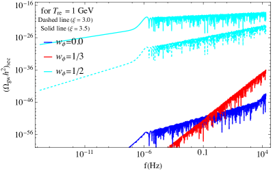
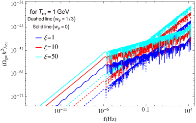
Figure 4: In this figure, we have shown the present-day dimensionless gravitational waves energy density $(\Omega_{\rm gw}h^{2})_{\rm sec}$ (induced by the scalar field only) as a function of frequency $f$ (Hz). The left panel illustrates the dependency of the EoS $w_{\phi}=0,1/3,~{}\&~{}1/2$ for two specific values of the coupling constant $\xi=3.5$ (indicated by solid lines) and $\xi=3.0$ (indicated by dashed lines). In the right panel, we have shown how the spectral energy density evolves for the coupling constants $\xi=1,10,~{}\&~{}50$, with fixed EoS values $w_{\phi}=0$ (indicated by solid lines) and $w_{\phi}=1/3$ (indicated by dashed lines). In both panels, we have considered the reheating temperature of our universe to be $T_{\rm re}=1$ GeV.

As is well-established, the energy density of gravitational waves (GWs) exhibits a behavior akin to radiation, scaling as $\rho_{\rm gw}\propto a^{-4}$. Our focus lies on modes that are well within the Hubble radius at a later time, particularly in proximity to the radiation-matter equality epoch during radiation domination. We express the dimensionless energy density parameter $\Omega_{\rm gw}(k)$ today in terms of $\Omega_{\rm gw}(k,\eta)$ as follows, as described in Haque et al. (2021); Maiti et al. (2024):

$$\Omega_{\rm gw}(k)h^{2} =\left(\frac{g_{r,eq}}{g_{r,0}}\right)\left(\frac{g_{s,0}}{g_{s,eq}}\right)^{4/3}\Omega_{R}h^{2}\Omega_{\rm gw}(k,\eta)\approx\left(\frac{g_{r,0}}{g_{r,eq}}\right)^{1/3}\Omega_{R}h^{2}\Omega_{\rm gw}(k,\eta).$$ (80)

Here, $\Omega_{R}h^{2}=4.3\times 10^{-5}$, representing the dimensionless energy density of radiation at the present epoch. $g_{r,eq}$ and $g_{r,0}$ represent the number of relativistic degrees of freedom at radiation-matter equality and in the present era, respectively, whereas $g_{s,eq}$ and $g_{s,0}$ signify the number of such degrees of freedom contributing to entropy at these respective epochs. In our calculation we adopt the values $g_{r,eq}\simeq g_{s,eq}=106.7$ and $g_{r,0}\simeq g_{s,0}=3.35$.

Primary GWs spectrum today(PGWs):

After the reheating epoch, the subsequent era is predominantly characterized by radiation. Now utilizing Eqs (70) and (78) in Eq.(80) we have found that the PGWs today can be estimated as Maiti et al. (2024)

$$\Omega_{\rm gw}^{\rm pri}(k)h^{2}\simeq 1.12\cdot 10^{-17}\left(\frac{\Omega_{R}h^{2}}{4.3\times 10^{-5}}\right)\left(\frac{H_{\rm end}}{10^{-5}{M}_{pl}}\right)^{2}\times\left\{\begin{matrix}\mathcal{D}_{1}&&\mbox{ for}~{}~{}k<k_{\rm re}\\ \mathcal{D}_{2}(k/k_{\rm re})^{n_{w}}&&\mbox{ for}~{}~{}k_{\rm re}<k<k_{\rm end}\end{matrix}\right..$$ (81)

Here, we introduce the parameter $n_{w}=2(3w_{\phi}-1)/(1+3w_{\phi})$, and define $\mathcal{D}_{1}=\pi^{2}2^{2l}/4\sin^{2}(l\pi)\Gamma^{2}(l)\Gamma^{2}(1-l)\simeq\mathcal{O}(1)$ and $\mathcal{D}_{2}\simeq\left(\pi^{2}/2\sin^{2}(l\pi)\Gamma^{2}(l)\right)\cos^{2}\left(-k/k_{\rm re}+(1-2l)\pi/4\right)\simeq\mathcal{O}(1)$.

Secondary GWs spectrum today(SGWs):

Similarly, using Eqs. (74) and (78) in Eq.(80) we have found that the secondary GWs spectrum for the modes $k_{\star}\leq k\leq k_{\rm end}$ can be estimated as

$$\Omega_{\rm gw}^{\rm sec}(k)h^{2}\simeq 2.22\times 10^{-26}\left(\frac{\Omega_{R}h^{2}}{4.3\times 10^{-5}}\right)\left(\frac{H_{\rm end}}{10^{-5}{M}_{pl}}\right)^{4}{\mathcal{A}^{2}}\left(1+\frac{k^{2}}{k_{\rm re}^{2}}\right)\left(\frac{k}{k_{\rm end}}\right)^{4+2\delta-4\nu_{2}}\mathcal{I}_{t}^{2}(k,\eta_{\rm re})\mathcal{F}(k)$$ (82)

In this context, $\mathcal{I}_{t}(k,\eta_{\rm re})$ represents the time integral as defined in Eq. (76), while $\mathcal{A}$ denotes the constant coefficient consisting of the EoS parameter and coupling strength ($w_{\phi},~{}\xi)$, as outlined in Eq. (75). We consider two distinct regimes to analyze the spectral behavior of secondary gravitational waves: $k\ll k_{\rm re}$ and $k_{\rm re}\ll k<k_{\rm end}$. In the super-horizon limit, the SGW spectrum follows the relation $\Omega_{\rm gw}^{\rm sec}(k\ll k_{\rm re})h^{2}\propto f^{4(2-\nu_{2})}$. In contrast, in the sub-horizon limit, the spectrum exhibits a behavior of $\Omega_{\rm gw}^{\rm sec}(k\gg k_{\rm re})h^{2}\propto f^{6+\delta-4\nu_{2}}$ (for further details, refer to the Appendix A).

As previously discussed, for an EoS with $w_{\phi}>1/3$ and a coupling parameter $\xi>1/6$, a post-inflationary parametric instability arises in the scalar field $\chi$, and significantly enhances the overall production of the scalar field during the reheating era. On the contrary, in scenarios where $w_{\phi}\leq 1/3$, no such post-inflationary instability occurs. In Fig. (4), we showed how such growths are imprinted in SGWs depending upon $w_{\phi}$ and the coupling parameter $\xi$. In the left panel, we examine three EoS values: $w_{\phi}=0$, $1/3$, and $1/2$, with a fixed reheating temperature of $T_{\rm re}=1$ GeV. The secondary GW spectrum generically acquires a common factor $\Omega_{\rm gw}^{\rm sec}(k)h^{2}\propto(k_{\rm end}/k_{\rm re})^{\frac{6w_{\phi}-2}{1+3w_{\phi}}}$ (see the detailed calculation in appendix A). The factor immediately suggests that for $w_{\phi}<1/3$ $(w_{\phi}>1/3)$, the amplitude of the spectrum is significantly suppressed (enhanced) as $k_{\rm end}/k_{\rm re}>>1$. This suppression or enhancement can indeed be seen from the left panel of Fig. 4. Detailed calculation further indicates that when $w_{\phi}\leq 1/3$, the secondary GW production is always overshadowed by the primary production for all scales. However, for $w_{\phi}=1/2$ (i.e., $w_{\phi}>1/3$), the production of SGWs due to the scalar field is significantly enhanced in super-horizon modes, potentially surpassing the primary gravitational wave production.

In the top left panel of Fig. 5, we explore the dependency of the coupling parameter $\xi$ for two different EoS values: $w_{\phi}=0$ and $1/3$. As neither of these EoS values induces instability in the system, no growth in the scalar field occurs during the reheating era (see Fig. 1). Consequently, the secondary production of gravitational waves is negligible, and the strength of the gravitational wave spectrum remains considerably lower than that of the primary gravitational waves, even when a very high coupling constant $\xi$ is considered.

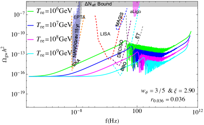
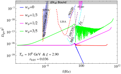
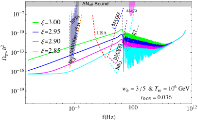
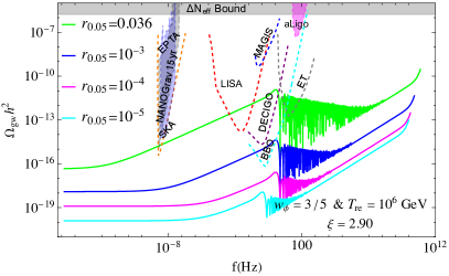
Figure 5: The figure presents the combined GW spectrum today for different theory parameters. In the top-left panel, we illustrate the dependence of the GW spectrum on the reheating temperature $T_{\rm re}$ for a fixed EoS $w_{\phi}=3/5$ with a coupling parameter $\xi=3.0$. The top-right panel shows the GW spectra for four different EoS values: $w_{\phi}=0,1/3$, $1/2$, and $3/5$, assuming a fixed reheating temperature of $T_{\rm re}=10^{6}$ GeV and a coupling constant $\xi=2.90$. The bottom-left panel demonstrates the influence of the coupling constant $\xi$ on the GW spectrum, where we assume a fixed reheating scenario with $T_{\rm re}=10^{6}$ GeV and $w_{\phi}=3/5$. In all three of these plots, we have adopted the maximal allowed value of the tensor-to-scalar ratio, $r_{0.05}\simeq 0.036$, as constrained by the Planck observations. Finally, in the bottom-right panel, we explore the impact of varying the tensor-to-scalar ratio on the GW spectrum for a fixed reheating scenario with $T_{\rm re}=10^{6}$ GeV, $w_{\phi}=3/5$, and $\xi=2.90$.

To this end, we would like to discuss the generic characteristics of the total GW spectrum (PGWs + SGWs) in terms of the reheating parameters, non-minimal coupling, and the inflationary energy scale. In the top left panel, we show the dependency of the reheating temperature on the GW spectrum, with a fixed equation of state $w_{\phi}=3/5$ and a coupling constant $\xi=2.90$. Evidently, in the intermediate frequency range, the secondary production of GWs can surpass the primary gravitational waves (PGWs). The decreasing temperature turns out to increase the overall amplitude of the spectrum through the factor $\Omega_{\rm gw}(k)h^{2}\propto T_{\rm re}^{\frac{8(1-3w_{\phi})}{3(1+w_{\phi})}}\propto T_{\rm re}^{~{}-4/3}$ for $k<k_{\rm re}$, $w_{\phi}=3/5$, and $\Omega_{\rm gw}(k)h^{2}\propto T_{\rm re}^{\frac{4(1-3w_{\phi})}{3(1+w_{\phi})}}\propto T_{\rm re}^{~{}-2/3}$ for $k>k_{\rm re}$, $w_{\phi}=3/5$. Beyond a certain reheating temperature, however, the large-scale spectrum can exceed the present bound on the tensor-to-scalar ratio $r_{0.05}\leq 0.036$ from the recent Planck-2018 results Aghanim et al. (2020), which we discuss in the subsequent section. The spectrum can intersect with future GW sensitivity curves for specific parameter sets, such as LISA, DECIGO, and BBO.

This enhancement of the SGWs with decreasing reheating temperature is effective only for $w_{\phi}>1/3$ reheating scenarios due to post-inflationary instability to the scalar field mode. Further lowering the reheating temperature implies an increase in the duration of the reheating period. A longer reheating period implies that the scalar field experiences instability for a more extended period, resulting in greater growth.

Similarly, in the top right panel of Fig. 5, we show the evolution of the final GW spectrum for different EoS values, indicated by four different colors. We assume $\xi=2.90$ and $T_{\rm re}=10^{6}$ GeV. For $w_{\phi}=0,1/3,1/2$ the PGW dominates the entire spectrum. Although for $w_{\phi}>1/3$ and $\xi>1$, there is instability in field growth (as seen in Fig.1), this growth is insufficient to produce significant GWs to surpass the PGWs generated during inflation due to quantum fluctuations. SGW turns out to dominate only when $w_{\phi}\geq 3/5$. For example assuming $w_{\phi}=3/5$ the spectrum transforms from scale-invariant to blue tilted in the small frequency(large scale) range $f^{8-4\nu_{2}}=f^{0.41}$, and from blue tilted to red-tiled $f^{6+\delta-4\nu_{2}}=f^{-0.16}$ for the modes $k>k_{\rm re}$(small scale) as indeed observed in green curve. Therefore, for a fixed reheating temperature and coupling constant $(\xi>1)$, there exists a threshold EoS value above which the scalar field growth is sufficient to produce enough SGWs to overtake the PGWs.

In the bottom left panel of Fig. 5, we examine the effect of the coupling constant $\xi$, with a fixed equation of state $w_{\phi}=3/5$ and reheating temperature $T_{\rm re}=10^{6}$ GeV. The results show that increasing the coupling parameter enhances the scalar field’s growth due to system instability, thereby enhancing the GW spectrum. The spectral behavior is the same as the previous one with blue tilt in the small frequency(large scale) range $f^{8-4\nu_{2}}$, and red-til $f^{6+\delta-4\nu_{2}}$ for the modes $k>k_{\rm re}$(small scale) as indeed observed in the green curve. We observe that for fixed reheating scenarios (fixed reheating temperature and EoS), there is always a critical value of the coupling constant $\xi_{\rm max}$, above which the tensor fluctuations at large scales can be overproduced, crossing the present upper bound on the tensor-to-scalar ratio $r_{0.05}\leq 0.036$ set by the Planck collaboration.

In the bottom right panel of Fig. 5, we demonstrate how the gravitational wave (GW) spectrum energy density varies with the tensor-to-scalar ratio $r_{0.05}$ for a fixed reheating temperature of $T_{\rm re}=10^{6}$ GeV and a fixed EoS $w_{\phi}=3/5$, with the coupling parameter $\xi=2.90$. The inflationary energy scale $H_{\rm end}$ is directly related to the tensor-to-scalar ratio $r_{0.05}$ through the relation $H_{\rm end}=\pi{M}_{pl}\sqrt{r_{0.05}A_{s}/2}$, and since the GW spectral energy density is proportional to the fourth power of the inflationary energy scale ($\Omega_{\rm gw}h^{2}\propto H_{\rm end}^{4}$), a decrease in $r_{0.05}$ leads to a corresponding reduction in the amplitude of both primary and secondary GWs due to the factor $(H_{\rm end}/{M}_{pl})$.

For a fixed reheating temperature, lowering the inflationary energy scale by reducing $H_{\rm end}$ leads to a shorter reheating period (see Eq. (46)). The duration of this period is intimately tied to the growth of the scalar field. When the tensor-to-scalar ratio $r_{0.05}$ is reduced, it not only limits the growth of the scalar field during reheating but also affects its initial production during inflation since the scalar field’s amplitude depends on the inflationary energy scale. As a result, the overall amplitude of the gravitational wave (GW) spectrum decreases as $r_{0.05}$ is lowered.

Considering these factors, we find that with $r_{0.05}$, $w_{\phi}=3/5$, $T_{\rm re}=10^{6}$ GeV, and $\xi=2.9$, the tensor fluctuations are strong enough to be detected by future sensitivity curves like LISA, DECIGO, and BBO. However, with a lower value like $r_{0.05}=10^{-3}$, the amplitude is suppressed, allowing detection by DECIGO and BBO but not by LISA. For $r_{0.05}\leq 10^{-4}$, the signal is too weak to be detected by upcoming experiments. Therefore, the inflationary energy scale significantly impacts the production of secondary GWs via the scalar field dynamics.

In all figures, at very high-frequency ranges near $f_{\rm end}=(k_{\rm end}/2\pi)$, the spectrum follows the $\Omega_{\rm gw}h^{2}(f)\propto f^{n_{w}}$ Maiti et al. (2024); Haque et al. (2021) behavior, which is due to PGWs contributions at these frequencies. At very high frequencies, PGWs dominate over SGWs. As seen in Fig.(3), when the modes re-enter, the scalar field growth is gradually suppressed because the system’s instability becomes ineffective once the modes are inside the horizon. The instability-inducing source term $a^{\prime\prime}/a\sim 1/\eta^{2}$ decreases over time. Thus, modes deep inside the horizon evolve adiabatically, and the growth time is insufficient to produce significant anisotropy.

Constraining the coupling Constant $\xi$ from the tensor-to-scalar ratio:

We have discovered that for $w_{\phi}>1/3$ reheating scenarios, the scalar field undergoes a tachyonic instability beyond a threshold of the coupling constant $\xi$, particularly for the super-horizon modes. The significant growth of these super-horizon modes can generate a substantial amount of tensor fluctuations even at Cosmic Microwave Background (CMB) scales. These tensor fluctuations are sufficiently strong to produce a notable tensor-to-scalar ratio at CMB scales. The current observational bound on the tensor-to-scalar ratio at CMB scales is $r_{0.05}\leq 0.036$, as reported by the Planck-2018 observations Aghanim et al. (2020). By utilizing this bound on $r_{0.05}$, and assuming that all contributions originate from secondary sources (i.e., the scalar fields), we can impose a stringent constraint on the coupling parameter $\xi$ through the following equation

$$r_{0.05} \simeq\frac{2(1-4\xi)^{2}\mathcal{A}_{3}^{2}H_{\rm end}^{4}}{\pi^{4}{M}_{pl}^{4}}\left\{\frac{1}{2l(\delta-2)}+\frac{1}{4l(1-l)-2l\delta}\right\}^{2}\frac{8(1+2\nu_{2})}{15(3-\nu_{2})(4\nu_{2}-5)}$$

$$\times\left(\frac{90H_{\rm end}^{2}M_{pl}^{2}}{\pi^{2}g_{\rm re}T_{\rm re}^{4}}\right)^{\frac{2(3w_{\phi}-1)}{3(1+w_{\phi})}}\left(\frac{k_{\star}}{k_{\rm end}}\right)^{4(2-\nu_{2})}\leq 0.036$$ (83)

From Eq.(83), it is evident that the reheating dynamics with a specified reheating temperature $T_{\rm re}$ and the average equation of state $w_{\phi}$, has a very sensitive dependence on the maximum coupling strength $\xi_{\rm max}$ to prevent the overproduction of tensor fluctuations at the CMB scale. All the solid curves in Figure (6) depict maximum allowed values of $\xi_{\rm max}$ as a function of $w_{\phi}$ for different values of $T_{\rm re}$. And $\xi_{\rm max}$ represents the value of the coupling constant for a specific set of parameters exceeding which would result in the overproduction of tensor perturbations at the CMB scale, thereby affecting the current bound on the tensor-to-scalar ratio $r_{0.05}$ Aghanim et al. (2020). For instance, when $w_{\phi}=0.5$ and $T_{\rm re}=10^{-2}$ GeV, the maximum value of the coupling constant is $\xi_{\rm max}\simeq 3.73$. On the other hand, if the reheating temperature is $T_{\rm re}=10^{6}$ GeV with the same EoS, the bound turns out to be $\xi_{\rm max}\simeq 3.99$. The plot shows that $\xi_{\rm max}$ decreases with a reduction in the reheating temperature due to the prolonged duration of the reheating era. During reheating with $w_{\phi}>1/3$, the scalar field experiences tachyonic instability; thus, a lower reheating temperature, which implies a longer duration of the reheating period, leads to significant growth in super-horizon modes. We have listed the maximum allowed values of $\xi$ for different reheating temperatures and equation of state in Table 1. Evidently, $\xi_{\rm max}$ does not vary much for a wide range of $(T_{\rm re},w_{\phi},r_{0.05})$. It varies within $\sim(2,4)$.

$r_{0.05}=0.036$	$T_{\rm re}$ (GeV)	$w_{\phi}=1/2$	$w_{\phi}=3/5$	$w_{\phi}=2/3$	$w_{\phi}=5/7$	$w_{\phi}=3/4$	$w_{\phi}=7/9$	$w_{\phi}=4/5$	$w_{\phi}=9/11$
	$10^{-2}$	3.7312	2.7649	2.4506	2.2967	2.2065	2.1473	2.1056	2.0748
	$10^{2}$	3.8599	2.9034	2.5945	2.4451	2.3578	2.3008	2.2611	2.2318
	$10^{6}$	3.9955	3.0518	2.7514	2.6076	2.5247	2.4714	2.4342	2.4071
$r_{0.05}=10^{-4}$	$10^{-2}$	3.7950	2.8136	2.4935	2.3375	2.2461	2.1859	2.1443	2.1123
	$10^{2}$	3.9289	2.9569	2.6439	2.4922	2.4039	2.3463	2.3059	2.2765
	$10^{6}$	4.0691	3.1111	2.8068	2.6613	2.5779	2.5242	2.4859	2.4591

Table 1: In the above table, we have listed the $\xi_{\rm max}$ for discrete reheating scenarios where we fixed the EoS $w_{\phi}$ and reheating temperature $T_{\rm re}$. This bound is derived from Eq. (83) to avoid the overproduction of tensor perturbations at the CMB scale. Based on recent observations from Planck, We consider the upper bound on the tensor-to-scalar ratio to be $r_{0.05}=0.036$. We also show the slight variation of $\xi_{\rm max}$ with tensor-to-scalar ratio by considering another value at the CMB scale $r_{0.05}=10^{-4}$.

Constraining the Reheating Dynamics through $\Delta N_{\rm eff}$:

The total radiation density around the time of decoupling influences the cosmic microwave background (CMB). At that epoch, neutrinos comprised a significant fraction of the radiative energy, but additional radiation (such as dark radiation or primordial gravitational waves) may also impact the CMB spectrum. In this context, treating the $\chi$ field as dark radiation significantly affects the CMB spectra through the extra radiation component. The effective number of neutrino species, $N_{\rm eff}$, which represents the energy density stored in relativistic components (radiation), is defined as

$$\rho_{\rm ra}=\rho_{\gamma}+\rho_{\nu}+\rho_{\rm x}=\left[1+\frac{7}{8}\left(\frac{4}{11}\right)^{4/3}N_{\rm eff}\right]\rho_{\gamma}$$ (84)

where $\rho_{\gamma}$, $\rho_{\nu}$, and $\rho_{\rm x}$ are the energy densities of photons, neutrinos, and extra radiation components (massless scalar field $(\rho_{\chi})$ or primordial gravitational waves $(\rho_{\rm gw})$), respectively. From Eq. (84), the excess radiation component can be defined as:

$$\rho_{\rm\chi}=\frac{7}{8}\left(\frac{4}{11}\right)^{4/3}\rho_{\gamma}\Delta N_{\rm eff}$$ (85)

where $\Delta N_{\rm eff}=N_{\rm eff}-N_{\nu}$ represents the extra relativistic degrees of freedom. Here, $\rho_{x}$ includes both dark radiation $\rho_{\chi}$ and primordial gravitational waves $\rho_{\rm gw}$, with $N_{\rm eff}$ being the observed total relativistic degrees of freedom and $N_{\nu}=3.044$ representing the standard model neutrino degrees of freedom Bennett et al. (2021); Froustey et al. (2020).

To determine the contribution of the dark radiation, specifically the massless scalar field $\chi$, we can express Eq. (85) as:

$$\rho_{\chi}=\frac{1}{2\pi^{2}}\int_{k_{\rm re}}^{k_{\rm end}}\frac{dk}{k}k^{4}|\beta_{k}|^{2}=\frac{7}{8}\left(\frac{4}{11}\right)^{4/3}\rho_{\gamma}\Delta N_{\chi}$$ (86)

where $\Delta N_{\chi}$ is the extra relativistic degree of freedom due to the dark radiation field $\chi$, for the sake of convenience, we introduce a new dimensionless variable $\Omega_{\chi}(\eta_{\rm re})=\rho_{\chi}(\eta_{\rm re})/\rho_{\rm c}(\eta_{\rm re})$, where $\rho_{\rm c}(\eta_{\rm re})=3H_{\rm re}^{2}{M}_{pl}^{2}$ is the background energy density at the end of reheating. As both the background energy density $(\rho_{c})$ and the massless scalar field (considered as dark radiation $\rho_{\chi}$) goes as $a^{-4}$ due the background expansion, the fractional energy density $\Omega_{\chi}(\eta>\eta_{\rm re}<\eta_{\rm eq})$ remain conserved during radiation dominated era. The present-day fractional energy density of the $\chi$ field can be expressed as

$$\Omega_{\chi}h^{2}\simeq\left(\frac{g_{r,0}}{g_{r,eq}}\right)^{1/3}\Omega_{\rm R}h^{2}\,\Omega_{\chi}(\eta_{\rm re})$$ (87)

where $\Omega_{\rm R}h^{2}\simeq 4.3\times 10^{-5}$ Aghanim et al. (2020) denotes the dimensionless energy density of radiation at the current epoch. Here, $g_{r,eq}$ and $g_{r,0}$ represent the number of relativistic degrees of freedom at the epochs of radiation-matter equality and the present day, respectively. By expressing Eq. (86) in terms of this dimensionless variable, we obtain

$$\Omega_{\chi}h^{2}=\frac{7}{8}\left(\frac{4}{11}\right)^{4/3}\Omega_{\gamma}h^{2}\Delta N_{\chi}\ \simeq 1.6\times 10^{-6}\left(\frac{\Delta N_{\chi}}{0.284}\right)$$ (88)

where $\Omega_{\gamma}h^{2}=2.47\times 10^{-5}$ is the present-day photon energy density Aghanim et al. (2020). The latest Planck data with Baryon Acoustic Oscillation (BAO) predicts $\Delta N_{\rm eff}\leq 0.284$ (within $2\sigma$ range) Aghanim et al. (2020). If we use this bound as an upper limit, we can tightly constrain the coupling parameter $\xi$ through Eq.(88).

In Fig.(6), we have plotted the upper limit of the coupling parameter $\xi_{\rm max}$ as a function of the average equation of state $w_{\phi}$ for five different reheating temperatures. Lowering the reheating temperature for a fixed EoS tightens the constraint on $\xi$. For example, if the EoS is $w_{\phi}=0.5$ and the reheating temperature of our universe is $T_{\rm re}=10^{-2}$ GeV, then to satisfy the current $\Delta N_{\rm eff}$ bound, the maximum allowed value of the coupling parameter is $\xi_{\rm max}\simeq 4.02$. Note this is greater than the bound we obtained from the tensor-to-ratio ($\xi_{\rm max}\simeq 3.73)$ discussed before. On the other hand, if the reheating temperature is $T_{\rm re}=10^{6}$ GeV with the same EoS, the bound is $\xi_{\rm max}\simeq 4.99$, which is again higher than the bound from the tensor to ratio ($\xi_{\rm max}\simeq 3.99)$ discussed before.

It is to be noted that combining constraints from the tensor-to-scalar ratio and from $\Delta N_{\rm eff}$ yields significant insights. In the lower reheating temperature case as one reduces the equation state the tensor to scalar ratio tends (solid lines) to provide stronger constraints on $\xi_{\rm max}$ than the $\Delta N_{\rm eff}$, and $\Delta N_{\rm eff}$ leads to the maximum possible value of equation state $w_{\phi}$ (set by dashed lines). For instance, with $w_{\phi}=0.6$ and a reheating temperature of $T_{\rm re}=10^{-2}$ GeV, the $\Delta N_{\rm eff}$ constraint predicts a maximum allowable value of the coupling constant $\xi_{\text{max}}\simeq 0.205$. In contrast, under the same reheating parameters, the tensor-to-scalar ratio constraint allows a higher upper bound for the coupling constant, $\xi_{\text{max}}\simeq 2.765$. Therefore, we get an allowed region of $\xi$ bounded by solid and dashed lines which satisfy both the constraints. This is indeed the case for red, blue, and magenta curves as depicted in the Fig.6 for $T_{\rm re}=(10^{-2},10^{2},10^{6})$ GeV accordingly. However, with the higher temperature, the constraint from PLANCK on tensor to scalar ratio becomes increasingly important and tends to prove the entire bound on $\xi$. This indeed can be observed for cyan and brown curves with $T_{\rm re}=(10^{14},10^{10})$ GeV respectively.

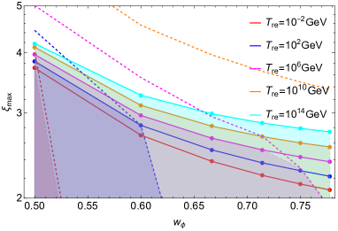
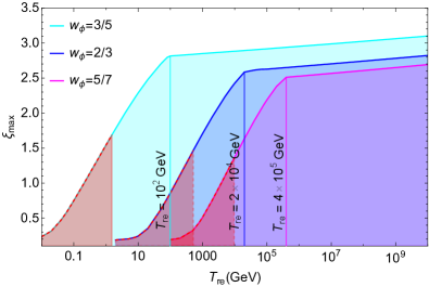
Figure 6: In the left panel, we present the maximum allowed values of the coupling constant, $\xi_{\rm max}$, as a function of $w_{\phi}$. The colored dashed lines represent $\xi_{\rm max}$ values calculated from the $\Delta N_{\rm eff}$ bound (see Eq. (88)). In contrast, the solid colored lines indicate the limit derived from the tensor-to-scalar ratio (see Eq. (83)). Different colors represent different $T_{\rm re}$ values. By combining both limits, we identify a common region allowed under both bounds, represented by the shaded areas corresponding to each color. In the right panel, we plot $\xi_{\rm max}$ as a function of $T_{\rm re}$ for three discrete values of the equation of state: $w_{\phi}=3/5$ (cyan), $w_{\phi}=2/3$ (blue), and $w_{\phi}=5/7$ (magenta). Combining both constraints, this plot shows the common allowed region, free from the $\Delta N_{\rm eff}$ and the tensor-to-scalar ratio bounds. The three vertical lines labeled by specific $T_{\rm re}$ values divided the shaded regions into two. Above this temperature, the tensor-to-scalar ratio imposes a stricter constraint on the coupling parameter $\xi$ compared to the $\Delta N_{\rm eff}$ bound. Three red-shaded regions indicate that these reheating temperatures are not allowed for the specified set of $w_{\phi}$ values as it violates $\Delta N_{\rm eff}$ bound at high frequency near $k_{\rm end}$ primarily sourced by PGWs.

Similarly, primordial gravitational waves (PGWs) with frequencies $\geq 10^{-15}$ Hz may contribute significantly to the radiation density of the Universe during the decoupling of the cosmic microwave background (CMB). It can also be treated as an extra relativistic degree of freedom symbolized as $\Delta N_{\rm gw}$. Hence, we can similarly express it as Caprini and Figueroa (2018); Maiti et al. (2024)

$$\Omega_{\rm gw}h^{2}=\frac{7}{8}\left(\frac{4}{11}\right)^{4/3}\Omega_{\gamma}h^{2}\Delta N_{\rm gw}\simeq 1.6\times 10^{-6}\left(\frac{\Delta N_{\rm gw}}{0.284}\right)$$ (89)

where $\Omega_{\rm gw}h^{2}$ is the present-day dimensionless energy density of the gravitational waves produced in the early universe and it is defined as

$$\Omega_{\rm gw}h^{2}=\int_{k_{\rm min}}^{k_{\rm end}}\frac{dk}{k}\Omega_{\rm gw}(k)h_{0}^{2}$$ (90)

here $\Omega_{\rm gw}(k)h^{2}$ is the total contributions from both primary and secondary gravitational waves. To this end, we should point out that the GW is a secondary contribution

Assuming the present-day photon density parameter is $\Omega_{\gamma}h^{2}\simeq 2.47\times 10^{-5}$, a combination of the latest Planck-2018 and Baryon Acoustic Oscillation (BAO) data predicts $\Delta N_{\text{eff}}\simeq 0.284$ (within a $2\sigma$ range) Aghanim et al. (2020). Consequently, this prediction sets an upper limit on primordial gravitational waves, such that $\Omega_{\rm gw}h^{2}<1.6\times 10^{-6}$ Clarke et al. (2020). Using this result, we derive the following inequality Smith et al. (2006); Clarke et al. (2020); Maiti et al. (2024)

$$\Omega_{\rm gw}h^{2}\leq 1.6\times 10^{-6}\left(\frac{\Delta N_{\rm gw}}{0.284}\right)$$ (91)

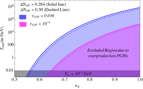
Figure 7: The figure above shows the minimum allowed reheating temperature $T_{\text{min}}$ (in GeV) as a function of $w_{\phi}$. The blue lines correspond to $r_{0.05}=0.36$, while the magenta lines represent $r_{0.05}=10^{-4}$. The solid lines indicate $\Delta N_{\rm eff}=0.284$, and the dashed lines indicate $\Delta N_{\rm eff}=0.50$. The shaded regions in color mark areas were excluded due to the overproduction of primary gravitational waves at the high-frequency end $f=f_{\rm end}({k_{e}}/{2\pi})$. The gray region at the bottom is excluded due to the minimum reheating temperature required by Big Bang NuclEoSynthesis (BBN), which is about $T_{\rm re}\simeq 10^{-2}$ GeV.

The constraint presented in Eq. (91) imposes a constraints on the reheating temperature;

$$T_{\text{min}}\geq\left(\frac{90H_{\rm end}^{2}M_{pl}^{2}}{\pi^{2}g_{\text{re}}}\right)^{1/4}\beta^{\frac{3(1+w_{\phi})}{4(3w_{\phi}-1)}}\left(\frac{0.284}{\Delta N_{\rm gw}}\right)^{\frac{3(1+w_{\phi})}{4(3w_{\phi}-1)}}$$ (92)

Here $T_{\text{min}}$ is the lowest possible reheating temperature to ensure the overproduction of the extra relativistic degree of freedom due to the PGWs. In the above we defined $\beta=1.43\times 10^{-11}\mathcal{D}_{2}(H_{\rm end}/10^{-5}M_{pl})^{2}/(n_{w})$. It is crucial to emphasize that this lower bound on the reheating temperature applies exclusively to the equation of state $w_{\phi}>1/3$.

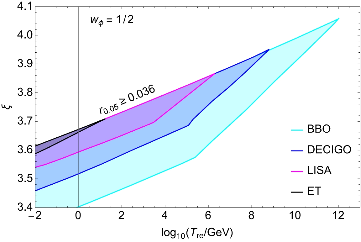
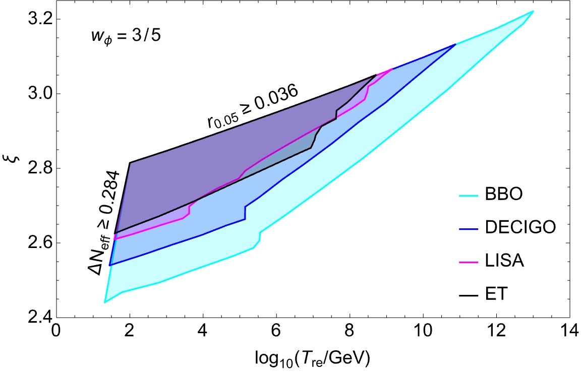
Figure 8: In the figure above, we present the estimated parameter space of the coupling constant $\xi$ versus the reheating temperature $T_{\rm re}$ for two different equations of state (EoS): $w_{\phi}=1/2$, and $w_{\phi}=3/5$. These estimates can be tested by future gravitational wave (GW) detectors, including LISA (magenta), DECIGO (blue), BBO (cyan), and ET (gray). Within this parameter space, the signal generated by the scalar field $\chi$ can be detected by these GW experiments. In both plots, the upper bound comes from the tensor to scalar ratio at the CMB scale where in the right panel at a lower temperature the $\Delta N_{\rm eff}$ puts a stronger constraint on the coupling parameter $\xi$.

Using Eq. (92), we have generated a parameter space plot of $T_{\text{min}}$ as a function of the average equation of state ($w_{\phi}$) in Fig. (7), showing the minimum permissible reheating temperature as a function of $w_{\phi}$. In this figure, the blue lines correspond to $r_{0.05}=0.036$, and the magenta lines to $r_{0.05}=10^{-4}$. Solid lines represent $\Delta N_{\rm eff}=0.284$, while dashed lines correspond to $\Delta N_{\rm eff}=0.50$. The shaded regions indicate areas excluded due to the overproduction of gravitational waves at high frequencies. The gray shaded region at the bottom excludes reheating temperatures lower than the BBN bound, i.e., $T_{\rm re}^{\rm BBN}\simeq 10^{-2}$ GeV. While considering a stiff equation of state ($w_{\phi}>1/3$), this bound must be taken into account. In all our plots, we have ensured that this bound is respected to avoid the overproduction of gravitational waves from primary quantum fluctuations during inflation.

Constraining Reheating Dynamics and Coupling Parameters $\xi$ via Future Gravitational Wave Experiments:

As depicted in Fig. (5), for an appropriate set of reheating parameters and coupling constant $\xi$, the production of secondary gravitational waves (SGWs) by the scalar field is significant enough to pass through the sensitivity curves of several forthcoming gravitational wave (GW) detectors, including LISA, DECIGO, BBO, ET, and others. This observation suggests that future GW detectors could probe non-minimal coupling and associated dynamics in the early universe, potentially placing stringent constraints on the coupling parameter $\xi$ and the reheating dynamics. In this section, we point out the parameter space in which these detectors are expected to explore these dynamics.

Focusing on future GW experiments such as LISA, DECIGO, BBO, and ET, we utilize the proposed sensitivity curves to estimate the parameter ranges for $\xi$ and the reheating temperature $T_{\rm re}$ for two different equations of state, $w_{\phi}=1/2$ and $w_{\phi}=3/5$, as shown in Fig. (8). The shaded regions indicate the parameter space where the signal produced by the scalar field is expected to be detectable by these experiments, provided $\xi$ falls within the specified range for a given reheating temperature and equation of state. Notably, the upper bound on $\xi$ remains the same for all experiments, despite differing sensitivity thresholds. This is because the upper limit on $\xi$ is determined by the tensor-to-scalar ratio constraint by PLANCK and the $\Delta N_{\rm eff}$ bound (as illustrated in Fig. (6)). Consequently, for values of $\xi$ exceeding a certain threshold, the signal, although potentially detectable, is excluded due to the overproduction of tensor fluctuations and additional relativistic degrees of freedom.

In the right panel of Fig. (8), we observe that when the reheating temperature is relatively low and the scalar field is considered as dark radiation, $\Delta N_{\rm eff}$ imposes stricter constraints on $\xi$, as discussed earlier. Conversely, in the case of $w_{\phi}=0.5$ (see in the left panel of Fig.(8)), the tensor-to-scalar ratio constraint is more restrictive than the $\Delta N_{\rm eff}$ constraint. For all the plots the lower boundary is fixed by the lowest values of the gravitational wave strength (sensitivity line) that a particular experiment could measure.

IV Conclusion

Over the past two decades, significant progress has been made in observational cosmology, enhancing our understanding of the universe and its evolutionary trajectories. However, the reheating epoch, a critical phase in cosmic history, remains poorly understood due to the lack of direct observational evidence. Reheating is a localized phenomenon, and information about its dynamics is obscured as the Standard Model (SM) plasma reaches local thermal equilibrium. Understanding how the universe achieves this thermal equilibrium is crucial for comprehending the physics of the early universe. Generally, this thermal bath is produced when the inflaton decays into SM particles, though the exact mechanisms of particle production at this stage are far from complete understanding.

In this study, we investigate the production of a massless scalar field in the presence of a $\xi R\chi^{2}$ coupling during both inflation and reheating. Our findings indicate that for $\xi>1/6$, although the scalar field production during inflation is negligible, post-inflationary instability can lead to significant growth of the scalar field, and this instability effect becomes important when the reheating equation of state parameter $w_{\phi}>1/3$ and the coupling constant $\xi\gtrsim 1$. Being driven by this instability effect, the scalar field’s growth suffices the purpose of inducing significant anisotropy, potentially sourcing secondary gravitational waves.

Our analysis shows that the gravitational waves produced during reheating can surpass the primary gravitational waves in an intermediate frequency range with specific parameter sets. Additionally, modes outside the horizon experience substantial growth; however, their growth rate decreases gradually upon horizon entry, and they evolve adiabatically over time. For $w_{\phi}>1/3$ reheating scenarios, owing to the strong post-inflationary instability effect, the amplification of the super-horizon modes generates enough tensor fluctuations even at the CMB scale to make an impact on the current constraints of the tensor-to-scalar ratio.

Our study deals with two important observational bounds, one is $\Delta N_{\rm eff}$ bound and another is the present-day tensor-to-scalar ratio bound at the CMB scale $r_{0.05}$, to restrict the maximum permissible range of the non-minimal coupling strength $\xi_{\rm max}$. The massless scalar field generating an appreciable anisotropy beyond a certain threshold of $\xi$ has been treated as a possible candidate for dark radiation. While discussing the $\Delta N_{\rm eff}$ bound, we have studied the individual contribution of two components(PGW, massless scalar $\chi$) to the present-day $\Delta N_{\rm eff}$ value. Except for a few reheating parameters($w_{\phi}$, $N_{\rm re},T_{\rm re}$), we have found a contrasting prediction of maximum coupling strength $\xi_{\rm max}$ made by these two observations as illustrated in Fig.(6). Furthermore, in the higher reheating temperature regime, we find stronger constraint from the tensor-to-scalar ratio bound that shrinks the maximum allowed region of $\xi$ for given reheating parameters. Finally, combining the latest Planck-2018 data of both $r_{0.05}$ and $\Delta N_{\rm eff}$, we put constraints on the coupling constant $\xi$. According to our present study, for $w_{\phi}\geq 1/2$, we find that the values $\xi>\xi_{\rm max}(\simeq 4)$ are disfavored by the combined set of recent observational bounds on the tensor-to-scalar ratio $r_{0.05}$ and $\Delta N_{\rm eff}$. Given the constraints from all the observations from PLANCK, towards the end, we derived the region of parameter space in $(T_{\rm re},\xi)$ plane which can be probed by future experiments such as BBO, DECIGO, LISA, and ET.

In connection with the aforementioned facts, our study upholds one important point: when the universe’s equation of state during reheating is $w_{\phi}>1/3$, arbitrarily large values of $\xi$ are hardly acceptable. Furthermore, specific parameter sets can produce distinctive gravitational wave signals detectable by future GW detectors, allowing for more robust constraints on the coupling parameters and reheating dynamics in the near future GW experiments.

V Acknowledgments

AC would like to thank the Ministry of Human Resource Development, Government of India (GoI), for financial assistance. SM gratefully acknowledges the financial support provided by the Council of Scientific and Industrial Research (CSIR), Ministry of Science and Technology, Government of India (GoI), through the Senior Research Fellowship (File No. 09/731(0192)/2021-EMR-I). DM wishes to acknowledge support from the Science and Engineering Research Board (SERB), Department of Science and Technology (DST), Government of India (GoI), through the Core Research Grant CRG/2020/003664.

Appendix A Computing the Secondary Tensor power spectrum:

We’ve shared here a detailed calculation for the tensor power spectrum during reheating for a generalized power law type matter power spectrum. Combining Eqs. (II.2.3) and (43) we can write the matter power spectrum in the following general form

$$\mathcal{P}_{X}(k,\eta)=\frac{k^{3}}{2\pi^{2}}\left|X^{\rm long}_{k}(k,\eta)\right|^{2}=\frac{\mathcal{A}_{3}}{\pi^{2}}~{}k_{\rm end}^{2}~{}\mathcal{I}(k,\eta)\left(\frac{k}{k_{\rm end}}\right)^{2(1-\nu_{2})}$$ (93)

In the above equation, $\mathcal{A}_{3}$ is a constant part depending on the initial parameters as given in (114) and $\mathcal{I}=\text{cos}^{2}(k\eta)$ is the time-dependent part of the matter power spectrum.

Now we can write the tensor power spectrum in terms of the matter power spectrum as

$$\mathcal{P}_{\rm T}^{\rm sec}(k,\eta_{\rm re})=\frac{8(1-4\xi)^{2}}{{M}_{pl}^{4}}\left(\int_{x_{\rm e}}^{x_{\rm re}}dx_{1}\frac{\mathcal{G}_{k}^{\rm re}(x_{\rm re},x_{1})}{a^{2}(x_{1})}\right)^{2}\times\int_{k_{\rm min}}^{k_{\rm end}}\frac{dq}{k}\int_{-1}^{1}d\gamma(1-\gamma^{2})^{2}\frac{(q/k)^{3}\mathcal{P}_{X}(q,\eta_{1})\mathcal{P}_{X}(|\bm{k}-\bm{q}|\eta_{1})}{|1-q/k|^{3}}$$ (94)

Now using Eq.(93) in the above Eq.(94) we get the following form.

$$\mathcal{P}_{\rm T}^{\rm sec}(k,\eta_{\rm re})= \frac{8(1-4\xi)^{2}\mathcal{A}_{3}^{2}k_{\rm end}^{4}}{\pi^{4}{M}_{pl}^{4}}\left(\int_{x_{\rm e}}^{x_{\rm re}}dx_{1}\frac{\mathcal{G}_{k}^{\rm re}(x_{\rm re},x_{1})}{a^{2}(x_{1})}\mathcal{I}(x_{1})\right)^{2}$$

$$\times\int_{k_{\rm min}}^{k_{\rm end}}\frac{dq}{k}\int_{-1}^{1}d\gamma(1-\gamma^{2})^{2}\frac{(q/k)^{3}(q/k_{\rm end})^{2(1-\nu_{2})}(|\bm{k}-\bm{q}|/k_{\rm end})^{2(1-\nu_{2})}}{|1-q/k|^{3}}$$ (95)

During the reheating era, the scale factor can be approximately written as $a^{2}(\eta)\approx a_{\rm end}^{2}(x/x_{\rm e})^{\delta}$, we recall that $\delta(w_{\phi})=4/(1+3w_{\phi})$. We obtain the following expression by substituting this approximate form of the scale factor to the above Eq.(95).

$$\mathcal{P}_{\rm T}^{\rm sec}(k,\eta_{\rm re}) =\frac{8(1-4\xi)^{2}\mathcal{A}_{3}^{2}H_{\rm end}^{4}}{\pi^{4}{M}_{pl}^{4}}\left(\frac{k}{k_{\rm end}}\right)^{4+2\delta-4\nu_{2}}\left(\int_{x_{\rm e}}^{x_{\rm re}}dx_{1}x_{1}^{-\delta}\mathcal{G}_{k}^{\rm re}(x_{\rm re},x_{1})\mathcal{I}(x_{1})\right)^{2}$$

$$\times\int_{k_{\rm min}}^{k_{\rm end}}\frac{dq}{k}\int_{-1}^{1}d\gamma(1-\gamma^{2})^{2}(q/k)^{5-2\nu_{2}}(|1-q/k|)^{-(1+2\nu_{2})}$$

$$=\frac{8(1-4\xi)^{2}\mathcal{A}_{3}^{2}H_{\rm end}^{4}}{\pi^{4}{M}_{pl}^{4}}\left(\frac{k}{k_{\rm end}}\right)^{4+2\delta-4\nu_{2}}\left(\underbrace{\int_{x_{\rm e}}^{x_{\rm re}}dx_{1}x_{1}^{-\delta}\mathcal{G}_{k}^{\rm re}(x_{\rm re},x_{1})\mathcal{I}(x_{1})}_{\text{Time Integral}}\right)^{2}\mathcal{F}(k)$$ (96)

where we define $\mathcal{F}(k)$ as

$$\mathcal{F}(k)=\int_{u_{\rm min}}^{u_{\rm max}}du\int_{-1}^{1}d\gamma(1-\gamma^{2})^{2}u^{5-2\nu_{2}}(1+u^{2}-2u\gamma)^{-(\nu_{2}+1/2)}$$ (97)

A.1 Computation of $\mathcal{F}(k)$ :

Here we define another variable $u=q/k$. In order to perform the momentum integral, we have to break it into two separate limits, i.e. $u_{\rm min}\leq u<1$ and $1<u\leq u_{\rm max}$, where $u_{\rm min}=k_{\rm min}/k$ and $u_{\rm max}=k_{\rm end}/k$ where $k_{\rm min}$ represents the largest observable scale as of today( CMB scale, $k_{\star}$) and $k_{\rm end}$ represent the largest mode that leaves the horizon at the end of inflation.

Now in the following range $u_{\rm min}\leq u<1$ the above integral (97) boils down to

$$\mathcal{F}_{1}\simeq\int_{u_{\rm min}}^{1}duu^{5-2\nu_{2}}\int_{-1}^{1}d\gamma(1-\gamma^{2})^{2}=\frac{16}{15(6-2\nu_{2})}\left\{1-\left(\frac{k_{\rm min}}{k}\right)^{6-2\nu_{2}}\right\}$$ (98)

where we have used $(1+u^{2}-2\gamma u)\simeq 1$. On the other hand for $1<u\leq u_{\rm max}$ range the above integral Eq.(97) boils down to the following one.

$$\mathcal{F}_{2} \simeq\int_{1}^{u_{\rm max}}du\int_{-1}^{1}d\gamma(1-\gamma^{2})^{2}u^{5-2\nu_{2}}u^{-(2\nu_{2}+1)}=\frac{16}{15(5-4\nu_{2})}\left\{\left(\frac{k_{\rm end}}{k}\right)^{5-4\nu_{2}}-1\right\}$$

$$=\frac{16}{15(5-4\nu_{2})}\left(\frac{k_{\rm end}}{k}\right)^{5-4\nu_{2}}\left\{1-\left(\frac{k}{k_{\rm end}}\right)^{5-4\nu_{2}}\right\}$$ (99)

where we have used $(1+u^{2}-2\gamma u)\simeq u^{2}$.

Now combining Eq.(98) and Eq.(99) we get

$$\mathcal{F}(k)=(\mathcal{F}_{1}+\mathcal{F}_{2})\simeq\frac{16}{15}\left\{\frac{1}{6-2\nu_{2}}\left(1-\left(\frac{k_{\rm min}}{k}\right)^{6-2\nu_{2}}\right)+\frac{1}{5-4\nu_{2}}\left(\left(\frac{k_{\rm end}}{k}\right)^{5-4\nu_{2}}-1\right)\right\}$$ (100)

A.2 Simplification of the Time Integral :

During reheating, the Green’s function of Eq.(54) is

$$\mathcal{G}_{k}^{\rm re}(x,x_{1})=\frac{\pi x^{l}x_{1}^{1-l}}{2\sin(l\pi)}(J_{l}(x)J_{-l}(x_{1})-J_{-l}(x)J_{l}(x_{1}))$$ (101)

We recall again $l(w_{\phi})=3(w_{\phi}-1)/2(1+3w_{\phi})$. Now using Eq.(101) we are going to perform the time integral part of Eq.(A)

$$\mathcal{I}_{t}(x_{\rm re},x_{\rm e})=\int_{x_{\rm e}}^{x_{\rm re}}dx_{1}x_{1}^{-\delta}\mathcal{I}(x_{1})\mathcal{G}_{k}^{\rm re}(x_{\rm re},x_{1})=\frac{\pi}{2\sin(l\pi)}\frac{x_{\rm re}^{l}x_{1}^{2-2l-\delta}}{2^{1+l}}\left(-x_{1}^{2l}J_{-l}(x_{\rm re})\Gamma\left[1-\frac{\delta}{2}\right]\right.$$

$$\left.\text{HypergeometricPFQRegularized}\left[\left\{1-\frac{\delta}{2}\right\},\left\{1+l,2-\frac{\delta}{2}\right\},-\frac{x_{1}^{2}}{4}\right]\right.$$

$$\left.\left.+4^{l}J_{l}(x_{\rm re})\Gamma\left[1-l-\frac{\delta}{2}\right]\text{HypergeometricPFQRegularized}\left[\left\{1-l-\frac{\delta}{2}\right\},\left\{1-l,2-l-\frac{\delta}{2}\right\},-\frac{x_{1}^{2}}{4}\right]\right)\right|_{x_{\rm e}}^{x_{\rm re}}$$ (102)

$$\mathcal{I}_{t}(x_{\rm re},x_{\rm e})=(\mathcal{I}_{t}(x_{\rm re},x_{\rm re})-\mathcal{I}_{t}(x_{\rm re},x_{\rm e}))\simeq\mathcal{I}_{t}(x_{\rm re},x_{\rm re})$$ (103)

For the sub-horizon limit i.e.

$$\mathcal{I}_{t}(x_{\rm re},x_{\rm e}) \simeq-\frac{\pi}{2\sin(l\pi)}\frac{2^{1-l-\delta}\pi}{\Gamma(l+\delta/2)\Gamma(\delta/2)}x_{\rm re}^{l}\left[\csc(\pi\delta/2)J_{-l}(x_{\rm re})-\csc\left[\pi(2l+\delta)/2\right]J_{l}(x_{\rm re})\right]$$

$$\simeq-\frac{2^{1-l-\delta}\pi\Gamma(1-l)\Gamma(l)}{2\Gamma(l+\delta/2)\Gamma(\delta/2)}x_{\rm re}^{l}\sqrt{\frac{2}{\pi x_{\rm re}}}\left\{\csc(\pi\delta/2)\cos\left[x_{\rm re}-\pi(1-2l)/4\right]-\csc\left[\pi(2l+\delta)/2\right]\cos\left[x_{\rm re}-\pi(1+2l)/4\right]\right\}$$

$$\simeq-\frac{2^{1-l-\delta}\pi\Gamma(1-l)\Gamma(l)}{2\Gamma(l+\delta/2)\Gamma(\delta/2)}x_{\rm re}^{l}\sqrt{\frac{2}{\pi x_{\rm re}}}$$ (104)

If we plug the above Eq.(104) into the Eq.(A) then we have the following

$$\lim_{k>>k_{\rm re}}\mathcal{P}_{\rm T}^{\rm sec}(k,\eta_{\rm re})\simeq\frac{2(1-4\xi)^{2}\mathcal{A}_{3}^{2}H_{\rm end}^{4}}{\pi^{4}{M}_{pl}^{4}}\frac{2^{1-2l-2\delta}\pi\Gamma^{2}(1-l)\Gamma^{2}(l)}{\Gamma^{2}(l+\frac{\delta}{2})\Gamma^{2}\left(\frac{\delta}{2}\right)}\frac{8(1+2\nu_{2})}{15(3-\nu_{2})(4\nu_{2}-5)}\left(\frac{k_{\rm re}}{k_{\rm end}}\right)^{\delta}\left(\frac{k}{k_{\rm end}}\right)^{4+\delta-4\nu_{2}}$$ (105)

Similarly for the super-horizon limit i.e. $x_{\rm re}<<1$ limit, the above integral boils down to the simplified form below.

$$\lim_{k<<k_{\rm re}}\mathcal{I}_{t}(x_{\rm re},x_{\rm e})\simeq x_{\rm re}^{2-\delta}\left\{\frac{1}{2l(\delta-2)}+\frac{1}{4l(1-l)-2l\delta}\right\}$$ (106)

Now utilizing this expression in Eq.(A) we obtain the tensor power spectrum at the super-horizon scale behaving as

$$\lim_{k<<k_{\rm re}}\mathcal{P}_{\rm T}^{\rm sec}(k,\eta_{\rm re})\simeq\frac{2(1-4\xi)^{2}\mathcal{A}_{3}^{2}H_{\rm end}^{4}}{\pi^{4}{M}_{pl}^{4}}\left\{\frac{1}{2l(\delta-2)}+\frac{1}{4l(1-l)-2l\delta}\right\}^{2}\mathcal{F}(k)\left(\frac{k_{\rm end}}{k_{\rm re}}\right)^{4-2\delta}\left(\frac{k}{k_{\rm end}}\right)^{4(2-\nu_{2})}$$

$$\simeq\frac{2(1-4\xi)^{2}\mathcal{A}_{3}^{2}H_{\rm end}^{4}}{\pi^{4}{M}_{pl}^{4}}\left\{\frac{1}{2l(\delta-2)}+\frac{1}{4l(1-l)-2l\delta}\right\}^{2}\frac{8(1+2\nu_{2})}{15(3-\nu_{2})(4\nu_{2}-5)}\left(\frac{k_{\rm end}}{k_{\rm re}}\right)^{4-2\delta}\left(\frac{k}{k_{\rm end}}\right)^{4(2-\nu_{2})}$$ (107)

GWs spectral behaviour for to extreme limit $k<<k_{\rm re}$ and $k>>k_{\rm re}$:

During the radiation-dominated era, the spectral energy density can be written as

$$\Omega_{\rm gw}(k,\eta)=\frac{\rho_{\rm gw}(k,\eta)}{\rho_{c}(\eta)}=\frac{1}{12}\frac{k^{2}\mathcal{P}_{\rm T}^{\rm rad}(k,\eta)}{a^{2}(\eta)H^{2}(\eta)}$$ (108)

where $\mathcal{P}_{\rm T}^{\rm rad}(k,\eta)$ is the tensor power spectrum during radiation dominated era and it can be written in terms of $\mathcal{P}_{\rm T}(k,\eta_{\rm re})$ as

$$\mathcal{P}_{\rm T}^{\rm rad}(k,\eta)=\left(1+\frac{k^{2}}{k_{\rm re}^{2}}\right)\frac{\mathcal{P}_{\rm T}(k,\eta_{\rm re})}{2k^{2}\eta^{2}}$$ (109)

Now utilizing Eq.(109) and (107) in Eq.(108) we obtain the at super-horizon limit the GW spectrum behaves as

$$\lim_{k<<k_{\rm re}}\Omega_{\rm gw}(k,\eta)\simeq\frac{2(1-4\xi)^{2}\mathcal{A}_{3}^{2}H_{\rm end}^{4}}{24\pi^{4}{M}_{pl}^{4}}\left\{\frac{1}{2l(\delta-2)}+\frac{1}{4l(1-l)-2l\delta}\right\}^{2}\frac{8(1+2\nu_{2})}{15(3-\nu_{2})(4\nu_{2}-5)}\left(\frac{k_{\rm end}}{k_{\rm re}}\right)^{4-2\delta}\left(\frac{k}{k_{\rm end}}\right)^{2(4-2\nu_{2})}$$ (110)

Similarly, for sub-horizon modes, the GW spectral energy density can be written as

$$\lim_{k>>k_{\rm re}}\Omega_{\rm gw}(k,\eta)\simeq\frac{2(1-4\xi)^{2}\mathcal{A}_{3}^{2}H_{\rm end}^{4}}{24\pi^{4}{M}_{pl}^{4}}\frac{2^{1-2l-2\delta}\pi\Gamma^{2}(1-l)\Gamma^{2}(l)}{\Gamma^{2}(l+\frac{\delta}{2})\Gamma^{2}\left(\frac{\delta}{2}\right)}\frac{8(1+2\nu_{2})}{15(3-\nu_{2})(4\nu_{2}-5)}\left(\frac{k_{\rm end}}{k_{\rm re}}\right)^{2-\delta}\left(\frac{k}{k_{\rm end}}\right)^{6+\delta-4\nu_{2}}$$ (111)

Appendix B Energy-density of Massless scalar field $\chi$ as a dark radiation component for $w_{\phi}>1/3$ :

In this section, we shall calculate the energy density of the dark radiation component employing the Eq.(86) with the knowledge of $\beta_{k}$ in different ranges of $\xi$ values for $w_{\phi}>1/3$ as calculated in Section II.

B.1 For $0\leq\xi<3/16$ :

In the given range $0\leq\xi<3/16$, the total energy density at the reheating end is computed to be

$$\rho_{\chi}\left(\frac{a}{a_{\rm end}}\right)^{4}=\frac{\mathcal{A}_{1}H_{\rm end}^{4}}{2\pi^{2}}\int_{k_{\rm re}/k_{\rm end}}^{1}d\left(k/k_{\rm end}\right)\left(k/k_{\rm end}\right)^{3-2(\nu_{1}+\nu_{2})}$$

$$\Rightarrow\rho_{\chi}\approx\frac{\mathcal{A}_{1}H_{\rm end}^{4}}{4\pi^{2}\left(2-(\nu_{1}+\nu_{2})\right)}\text{exp}(-4N_{\rm re})$$ (112)

where $\mathcal{A}_{1}=\left(\frac{\Gamma(\nu_{1})\Gamma(\nu_{2})2^{\nu_{1}}}{8\pi}\left(\frac{2}{3\mu-1}\right)^{\nu_{2}}\left(\frac{3\mu(1-2\nu_{1})+2(\nu_{1}-\nu_{2})}{\sqrt{(3\mu-1)}}\right)\right)^{2}$. For $w_{\phi}>1/3$, in this specified range of $\xi$, we always have $(4-2(\nu_{1}+\nu_{2}))>0$. So, the maximum contribution to energy is coming from $k_{\rm end}$. This property of the blue-tilted spectrum is used to reach the final expression of $\rho^{\rm com}_{\chi}$ in Eq.(B.1).

B.2 For $\xi=3/16$ :

Likewise the previous case, the total energy density at the reheating end for $\xi=3/16$ is evaluated to be

$$\rho_{\chi}\approx\frac{\mathcal{A}_{2}H_{\rm end}^{4}}{4\pi^{2}\left(2-\nu_{2}\right)}\text{exp}(-4N_{\rm re})$$ (113)

where $\mathcal{A}_{2}=\left(\frac{\Gamma(\nu_{2})}{2}\left(\frac{2}{3\mu-1}\right)^{\nu_{2}}\left|\frac{3\mu-2\nu_{2}}{4\sqrt{(3\mu-1)}}+\frac{i\sqrt{3\mu-1}}{\pi}\right|\right)^{2}$

B.3 For $\xi>3/16$ :

In this range, the existence of the critical coupling strength $\xi^{(1)}_{\rm cri}$ $\left(\text{a function of}~{}w_{\phi},~{}\xi^{(1)}_{\rm cri}=\frac{(9w_{\phi}+7)(15w_{\phi}+1)}{48(3w_{\phi}-1)}\right)$ of no. density spectrum $|\beta_{k}|^{2}$ distinguishes two regions with a junction that is at $\xi=\xi^{(1)}_{\rm cri}$.

B.3.1 For $3/16<\xi<\xi^{(1)}_{\rm cri}$ :

For $3/16<\xi<\xi_{\rm cri}^{(1)}$, the energy spectrum being blue-tilted again satisfies the same expressions of reheating parameters as in the range $0\leq\xi\leq 3/16$. The total energy density at the reheating end is computed as

$$\rho_{\chi}\approx\frac{\mathcal{A}_{3}H_{\rm end}^{4}}{4\pi^{2}\left(2-\nu_{2}\right)}\text{exp}(-4N_{\rm re})$$ (114)

where $\mathcal{A}_{3}\approx\left(\frac{\Gamma(\nu_{2})\text{exp}(-\pi\tilde{\nu}_{1}/2)}{4}\left(\frac{2}{3\mu-1}\right)^{\nu_{2}}\sqrt{3\mu-1}\left|\frac{\left(\pi+i\text{cosh}(\pi\tilde{\nu_{1}})\Gamma(1-i\tilde{\nu_{1}})\Gamma(i\tilde{\nu_{1}})\right)}{\pi\Gamma(i\tilde{\nu_{1}})}\right|\right)^{2}$

B.3.2 For $\xi=\xi^{(1)}_{\rm cri}$ :

At this junction point, the total energy density at the reheating end is computed as

$$\rho_{\chi}=\frac{\mathcal{A}_{3}H_{\rm end}^{4}}{2\pi^{2}}\text{ln}\left(\frac{k_{\rm end}}{k_{\rm re}}\right)\text{exp}(-4N_{\rm re})$$

$$\Rightarrow\rho_{\chi}=\frac{\mathcal{A}_{3}H_{\rm end}^{4}(1+3w_{\phi})N_{\rm re}}{4\pi^{2}}\text{exp}(-4N_{\rm re})$$ (115)

B.3.3 For $\xi>\xi^{(1)}_{\rm cri}$ :

After crossing the critical coupling or the junction $\xi_{\rm cri}^{(1)}$, the energy spectrum turns out to be red-tilted. The total energy density at the reheating end is now computed as

$$\rho_{\chi}=\frac{\mathcal{A}_{3}H_{\rm end}^{4}}{4\pi^{2}(\nu_{2}-2)}\left(\frac{k_{\rm end}}{k_{\rm re}}\right)^{2\nu_{2}-4}\text{exp}(-4N_{\rm re})$$

$$\Rightarrow\rho_{\chi}=\frac{\mathcal{A}_{3}H_{\rm end}^{4}}{4\pi^{2}(\nu_{2}-2)}\text{exp}\Big{(}\big{(}(1+3w_{\phi})(\nu_{2}-2)-4\big{)}N_{\rm re}\Big{)}$$ (116)