The Small Sizes and High Implied Densities of ‘Little Red Dots’ with Balmer Breaks Could Explain Their Broad Emission Lines Without an AGN

Abstract

Early JWST studies found an apparent population of massive, compact galaxies at redshifts $z\gtrsim 7$. Recently three of these galaxies were shown to have prominent Balmer breaks, demonstrating that their light at $\lambda_{\rm rest}\sim 3500$ Å is dominated by a stellar population that is relatively old ($\sim$200 Myr). All three also have broad H$\beta$ emission with $\sigma>1000\,\rm km\,s^{-1}$, a common feature of such ‘little red dots’. From Sérsic profile fits to the NIRCam images in F200W we find that the stellar light of galaxies is extremely compact: the galaxies have half-light radii of $r_{\rm e}\sim$ 100 pc, in the regime of ultra compact dwarfs in the nearby Universe. Their masses are uncertain, as they depend on the contribution of possible light from an AGN to the flux at $\lambda_{\rm rest}>5000$ Å. If the AGN contribution is low beyond the Balmer break region, the masses are $M_{*}\sim 10^{10}-10^{11}\mathrm{M}_{\astrosun}$, and the central densities are higher than those of any other known galaxy population by an order of magnitude. Interestingly, the implied velocity dispersions of $\sim$1500 km s^-1 are in very good agreement with the measured H$\beta$ line widths. We suggest that some of the broad lines in ‘little red dots’ are not due to AGNs but simply reflect the kinematics of the galaxies, and speculate that the galaxies are observed in a short-lived phase where the central densities are much higher than at later times. We stress, however, that the canonical interpretation of AGNs causing the broad H$\beta$ lines also remains viable.

1 Introduction

The James Webb Space Telescope (JWST) has revealed a population of high redshift objects with very specific spectral energy distributions (SEDs): a flat blue continuum and a steep red slope (e.g., Labbé et al., 2023a; Barro et al., 2024; Akins et al., 2024; Kocevski et al., 2023; Ono et al., 2023; Onoue et al., 2023; Labbé et al., 2023b). They are often compact (Akins et al., 2023; Baggen et al., 2023) (appearing as ‘little red dots’, LRDs; Matthee et al., 2024) and some, but not all, are confirmed to have moderately broad (FWHM $\sim$1200-4000 km s^-1) Balmer lines in their spectra (e.g., Kocevski et al., 2023; Matthee et al., 2024; Greene et al., 2024; Kokorev et al., 2023; Killi et al., 2023; Maiolino et al., 2023; Übler et al., 2023; Harikane et al., 2023a; Larson et al., 2023; Wang et al., 2024a, b; Kokorev et al., 2024). The most straightforward interpretation of the small sizes and broad Balmer lines is that we are seeing active galactic nuclei (AGN) with a broad line region (BLR). If they are AGN, they are unusual: they are typically not detected in X-ray emission (Ananna et al., 2024; Akins et al., 2024; Maiolino et al., 2024; Yue et al., 2024; Furtak et al., 2024; Greene et al., 2024; Kokubo & Harikane, 2024), have yet to demonstrate photometric variability in NIRCam (Kokubo & Harikane, 2024), have flat SEDs in the mid-far IR for some LRDs implying dominant contribution from stars at these wavelengths (Pérez-González et al., 2024), show no dominant contribution from hot dust emission expected from an AGN at rest-frame 3 $\mu$m (Williams et al., 2024), and have not been detected in stacks of mid-IR/far-IR/sub-mm/radio data (Akins et al., 2024).

The correct interpretation of these galaxies – whether they are dominated by AGNs or are compact and massive – has far-reaching implications for black hole physics (e.g. Greene et al., 2024; Maiolino et al., 2024; Bogdán et al., 2024; Kovács et al., 2024; Juodžbalis et al., 2024a; Inayoshi & Ichikawa, 2024), the theory of galaxy formation and evolution (e.g. Silk et al., 2024), and perhaps even cosmology (Boylan-Kolchin, 2023).

Recently, three LRDs at redshifts $z=6.8-8.4$ were shown to have prominent Balmer breaks in their JWST spectra (Wang et al., 2024b). Two of these galaxies are among the massive galaxy candidates reported in Labbé et al. (2023a). The Balmer break indicates the presence of an evolved stellar population, with stellar ages of more than 100 Myr (Bruzual A., 1983; Hamilton, 1985; Worthey et al., 1994; Balogh et al., 1999; Poggianti et al., 1999), and their detection strongly suggests that the SEDs at $\lambda_{\rm rest}\sim 3500$ Å are not dominated by AGNs. However, all three objects also have broad H$\beta$ emission lines ($\sigma_{\rm H\beta}>$1000 km s^-1), suggesting that AGNs are present. Wang et al. (2024b) fit the SEDs of the three galaxies, and show that the derived stellar population parameters depend sensitively on the interpretation of the continuum redward of the Balmer break. Equally good fits are obtained using either a model with a high stellar mass and extended SFH, a model with a dust-obscured AGN with minimal stellar mass, or a solution in between. This leads to a wide range of stellar masses ($M_{*}\sim 10^{9}-10^{11}\mathrm{M}_{\astrosun}$) and the implied possible natures and evolutionary tracks of these sources range from the progenitors of massive ellipticals to low-mass galaxies with over-massive black holes.

In this Letter, we use the fact that we know both the redshifts of these galaxies and that the extended light in the UV suggests that the light at these wavelengths is dominated by stars to measure accurate half-light radii. This follows our initial size measurements (Baggen et al., 2023) of the Labbé et al. (2023a) galaxies that were based on photometric redshifts and earlier versions of the imaging data. We then use the previously-determined masses for different AGN contributions, combined with the sizes, to measure densities and predict emission line widths and compare these to the observed line widths. Throughout this work we assume $\Lambda$CDM cosmology with $H_{0}$=70 km s^-1 Mpc^-1, $\Omega_{m,0}$=0.3 and $\Omega_{\Lambda,0}$=0.7. Magnitudes are reported in the AB system.

2 Data

2.1 Imaging

The JWST Near Infrared Camera (NIRCam) imaging data of this paper are obtained from the Cosmic Evolution Early Release Science (CEERS) program (PI: Finkelstein; PID: 1345 Finkelstein et al., 2022, 2023b) (see data DOI: Finkelstein et al., 2023a). In this work, we use the mosaics available through the DAWN JWST Archive (DJA, v7.2), which are reduced using the grizli pipeline (Brammer, 2023). The mosaics are available in six broadband filters, short-wavelength (SW; F115W, F150W, F200W) and long-wavelength (LW; F277W, F356W and F444W) with a resolution of $0\farcs 04$ pix^-1. In addition, higher resolution ($0\farcs 02$ pix^-1) data are available for the SW bands, for which the mosaics are split into 12 tiles. Ideally, we would use the band at the location of the Balmer break ($\sim 3\mu$m), to do the analysis. However, due to the large pixel size (and the broader PSF) of the LW data, the galaxies are barely resolved/unresolved at these wavelengths. Therefore, we use F200W for our analysis, the reddest band available with 20 mas sampling. Moreover, the F200W filter probes the highest SNR out of all the SW filters. We show cutouts and RGB images (see Figure 1) of the galaxies using multiple bands for illustration.

Compared to previous versions (e.g. v4 used in Labbé et al., 2023a; Baggen et al., 2023), the weighting scheme to do the drizzling has changed. Previously, the weighting was done including the Poisson noise from the source. This caused a suppressing of flux in the central pixels for compact sources, which could directly affect the sizes of sources in the images. As we will show in this work, the two sources (L23-38094, L23-14924) for which the sizes are also reported in Baggen et al. (2023), the newly measured sizes are indeed smaller in the new reductions.

The form of the point-spread function (PSF), that describes how point sources appear in the data, is a crucial aspect of the analysis, yet complicated to model properly. One approach is to create an empirical PSF from either bright well-centered single stars or by stacking multiple stars in the mosaic. Another approach is forward modeling of the telescopes instruments, such as what is done for the tool WebbPSF created for JWST imaging (Perrin et al., 2014). The advantage of these synthetic PSFs is high signal-to-noise ratios and perfect sampling. However, a variety of studies have found discrepancies between WebbPSF profiles and point sources in the images (Ding et al., 2022; Ono et al., 2023; Onoue et al., 2023; Weaver et al., 2023).

We first consider a PSF made from stacking of centered, bright, unsaturated stars in the entire mosaic (as described in Weibel et al., 2024). However, we find that this PSF gives large ellipticities (and a very similar position angle) when fit to compact galaxies. Furthermore, the light profile is clearly broader than that of single, well-centered stars in the vicinity of the three galaxies. Therefore we also consider five single stars (RA [214.958582, 214.950395, 214.97986, 214.827323, 214.802483], DEC [52.930525, 52.946655, 52.969334, 52.8194630, 52.837142]), that are bright and close to the galaxies. This method avoids smoothing due to stacking and implicitly accounts for local variations of the PSF. While these stars all give very similar results, none of the stars is perfectly centered ($>$0.1 pixel shift in x and y).

Finally, we inspect results from synthetic WebbPSF models. These fits are almost identical to those from single stars. Given the reproducability of WebbPSF, we use this for our reported measurements. The uncertainty in the PSF is taken into account in the error analysis, where we use both WebbPSF, single stars, and the stacked empirical PSF (see Section 3.3).

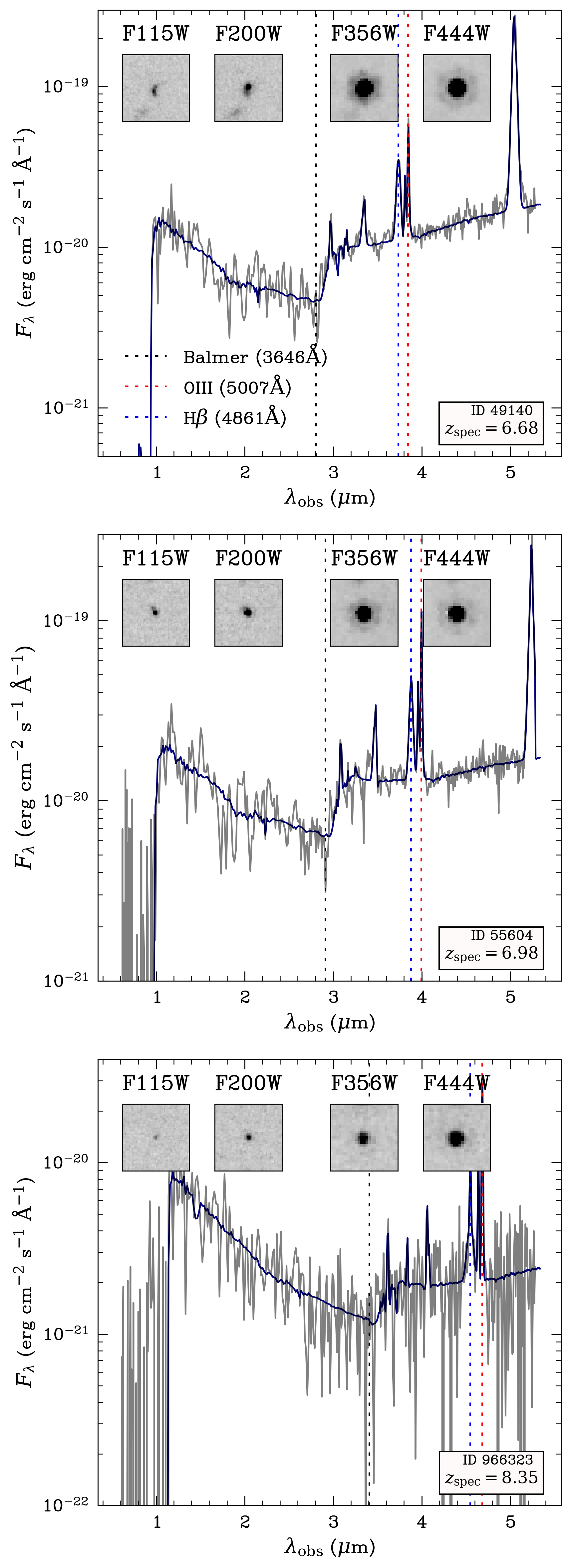
Figure 1: The spectra (grey) and best-fit model (darkblue) with maximal stellar mass of three Balmer break galaxies, obtained from Wang et al. (2024b). We also show $1\arcsec\times 1\arcsec$ images in four different bands, F115W, F200W, F356W and F444W. The dotted lines indicate the location of the Balmer break (black), OIII line (red), and H$\beta$ (blue) line, which are relevant in this work. For information on other emission lines, see Wang et al. (2024b).

RUBIES-ID	L23-ID	RA	DEC	$z_{\mathrm{spec}}$	$\log$($M_{*,\mathrm{max}}$)	$\log$($M_{*,\mathrm{med}}$)	$\log$($M_{*,\mathrm{min}}$)	$\sigma$(H$\beta$)	$r_{\mathrm{e,maj}}$	$b/a$
					[$\mathrm{M}_{\odot}$]	[$\mathrm{M}_{\odot}$]	[$\mathrm{M}_{\odot}$]	[km s-1]	[pc]
49140		214.89225	52.87741	6.68	11.2${}^{+0.15}_{-0.14}$	9.93${}^{+0.22}_{-0.14}$	9.50${}^{+0.08}_{-0.09}$	1402${}^{+68}_{-79}$	123${}^{+173}_{-45}$	0.58
55604	38904	214.98303	52.95600	6.98	11.1${}^{+0.15}_{-0.16}$	9.79${}^{+0.14}_{-0.14}$	8.99${}^{+0.16}_{-0.14}$	1527${}^{+106}_{-115}$	54${}^{+53}_{-43}$	0.78
966323	14924	214.87615	52.88083	8.35	10.6${}^{+0.13}_{-0.49}$	9.84${}^{+0.20}_{-0.32}$	8.72${}^{+0.21}_{-0.19}$	1369${}^{+280}_{-315}$	86${}^{+9}_{-42}$	0.73

Table 1: Spectroscopic and structural properties of three Balmer break galaxies. The first and second column indicate the galaxy ID given in Wang et al. (2024b) and the corresponding ID number of L23. The spectroscopic redshift (column 4), stellar masses ($\mathrm{M}_{\odot}$) with $1\sigma$ errors (columns 4-6) and velocity dispersion (km s^-1) of the broad H$\beta$ line (column 7) are obtained from Wang et al. (2024b). The three different stellar masses are obtained by varying the AGN contribution relative to stellar contribution (see text). The 8th and 9th column are the fitted effective radii $r_{\rm e,maj}$ (pc) along the major axis and the minor-to-major axisratio ($b/a$), respectively. The galaxies are fit with a Sérsic profile in filter F200W using WebbPSF. We perform simulations (see text) to obtain $1\sigma$ errors on the size measurements.

2.2 Spectra

The spectroscopic properties of the three LRDs with Balmer breaks shown in this paper are obtained from Wang et al. (2024b). Briefly, the galaxies were selected from a spectroscopic follow-up program RUBIES (JWST-GO-4233; PIs de Graaff & Brammer, de Graaff et al. in prep.), that uses the NIRSpec microshutter array (MSA). The double-break candidates of Labbé et al. (2023a) were targeted and observed in March 2024 for 48 min in the Prism/Clear mode and the G395M/F290LP mode. For more information on the reduction we refer to Heintz et al. (2024).

The modeling of the spectra is described in Wang et al. (2024b). Briefly, three different limiting cases are adopted to decompose the continuum into a stellar and AGN component. The first model maximizes the stellar contribution and minimizes the AGN contribution to the continuum, by setting it to zero. The resulting stellar masses of all three galaxies are very high, $M_{\mathrm{*,max}}\sim 10^{11}\mathrm{M}_{\odot}$. The second model assumes a maximal AGN contribution, and therefore minimizes the contribution of stars. These minimal masses are $M_{\mathrm{*,min}}\sim 10^{9}\mathrm{M}_{\odot}$. The third model lies somewhere in between, resulting in stellar masses $M_{\mathrm{*,med}}\sim 10^{10}\mathrm{M}_{\odot}$. Interestingly, while these three models are physically very different, they give equally good fits to the red continuum. In this work, following Wang et al. (2024b), we consider all three cases as possible truths. The nine individual mass measurements, taken from Wang et al. (2024b), are listed in Table 1.

In Figure 1 we show the spectra in light grey and the best-fit model using the maximum stellar mass in dark blue. For illustration we also show the Balmer break at $\lambda_{\rm rest}=3646\rm\AA$, the OIII line at $\lambda_{\rm rest}=5007\rm\AA$ and H$\beta$ at $\lambda_{\rm rest}=4861\rm\AA$ as dotted lines in black, red and blue, respectively.

3 Structural Properties

3.1 Morphologies

In Figure 2 (top panels) we show the individual images ($1\arcsec\times 1\arcsec$) for the three Balmer break galaxies in F200W, as well as the NIRSpec slits that were used. We also show two RGB images, the first created from cutouts in F115W (blue), F150W (green), F200W (red), the second from F150W (blue), F277W (green), F444W (red). The images show that all three galaxies are extremely small, and appear as single, unresolved or barely resolved objects in the long wavelength bands. However, the morphologies of two of the galaxies are more complex in the bluer bands. ID-49140 and ID-55604 have a faint extension or small clump next to a compact primary component. These clumps are most prominent in F115W (see cutout images in Figure 1). The morphology of ID-966323 is more point-like in all bands.

3.2 Sérsic Profile Fitting

We fit the surface brightness profiles of the three Balmer break galaxies with Sersic (1968) profiles. As explained in § 2.1 the fits are done in F200W, probing rest-frame wavelengths of $\lambda_{\rm rest}\sim 200-250$ nm. We use galfit (Peng et al., 2002, 2010), and the relevant parameters are the central position ($x$, $y$), the effective radius (along the major axis) ($r_{\rm e}$), the Sérsic index ($n$), the total integrated magnitude, projected minor-to-major axis ratio ($b/a$), and the position angle (PA).

Initial fits showed that the Sérsic index cannot be determined robustly, given the small sizes of the galaxies, but that it typically ranges between 1 - 3.5. We adopt a fixed $n=1.5$ in the fits. The uncertainty in $n$ translates into an uncertainty in $r_{\rm e}$, and this is propagated in our error analysis (see Section 3.3). The $r_{\rm e}$ is allowed to vary between 0.01 and 100 pixels and the total integrated magnitude between $-5$ and +5 magnitudes from the previously measured aperture magnitude.

We generate a mask with contaminating sources as follows. The background is estimated using sigma-clipped statistics with a filter size of 5 pixels and the background RMS ($\sigma$). After subtracting the background, the data are convolved with a 2D Gaussian kernel with a FWHM of 3 pixels. Using this convolved background-subtracted image, we adopt a source detection threshold of 1.5$\sigma$. The resulting map contains pixels that are not considered while fitting the galaxy models on the image with galfit.

For RUBIES-55604 and RUBIES-49140, we fit two Sérsic components based on the images in F115W and F150W (see Section 3.1). The nature of the relatively blue secondary, offset, components is unclear. The primary component contains 70 % and 85 % of the total fluxes of RUBIES-55604 and RUBIES-49140, respectively. As the primary components are redder than the secondary components (particularly for RUBIES-55604 – see Fig. 2), they contribute an even larger fraction of the total masses. Fitting the galaxies with single components leads to significant residuals, as expected, and sizes that are twice as large as our default values. We include this systematic uncertainty in the errorbars of these objects, as discussed below.

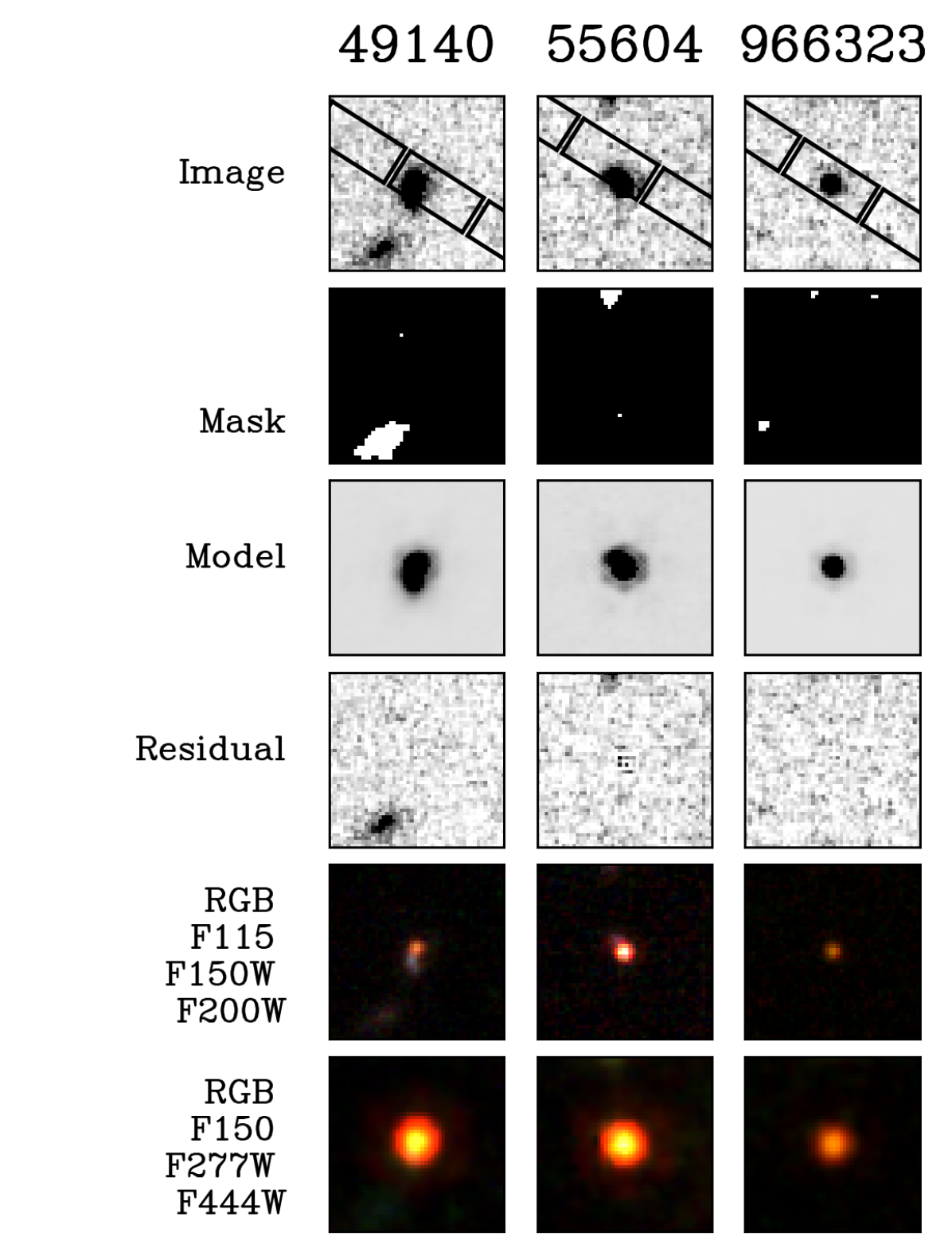
Figure 2: The top row shows images in the NIRCam F200W band of the three Balmer break galaxies. The second row shows the segementation maps, the third the best-fitting PSF convolved galfit models. The residuals, obtained by subtracting the best-fitting models from the images, are shown in the fourth row. The fifth row shows RGB images of the galaxies, with F115W as the blue band, F150W as the green band and F200W as the red band and the final row with F115W, F277W, F444W. All images are $1\arcsec\times 1\arcsec$.

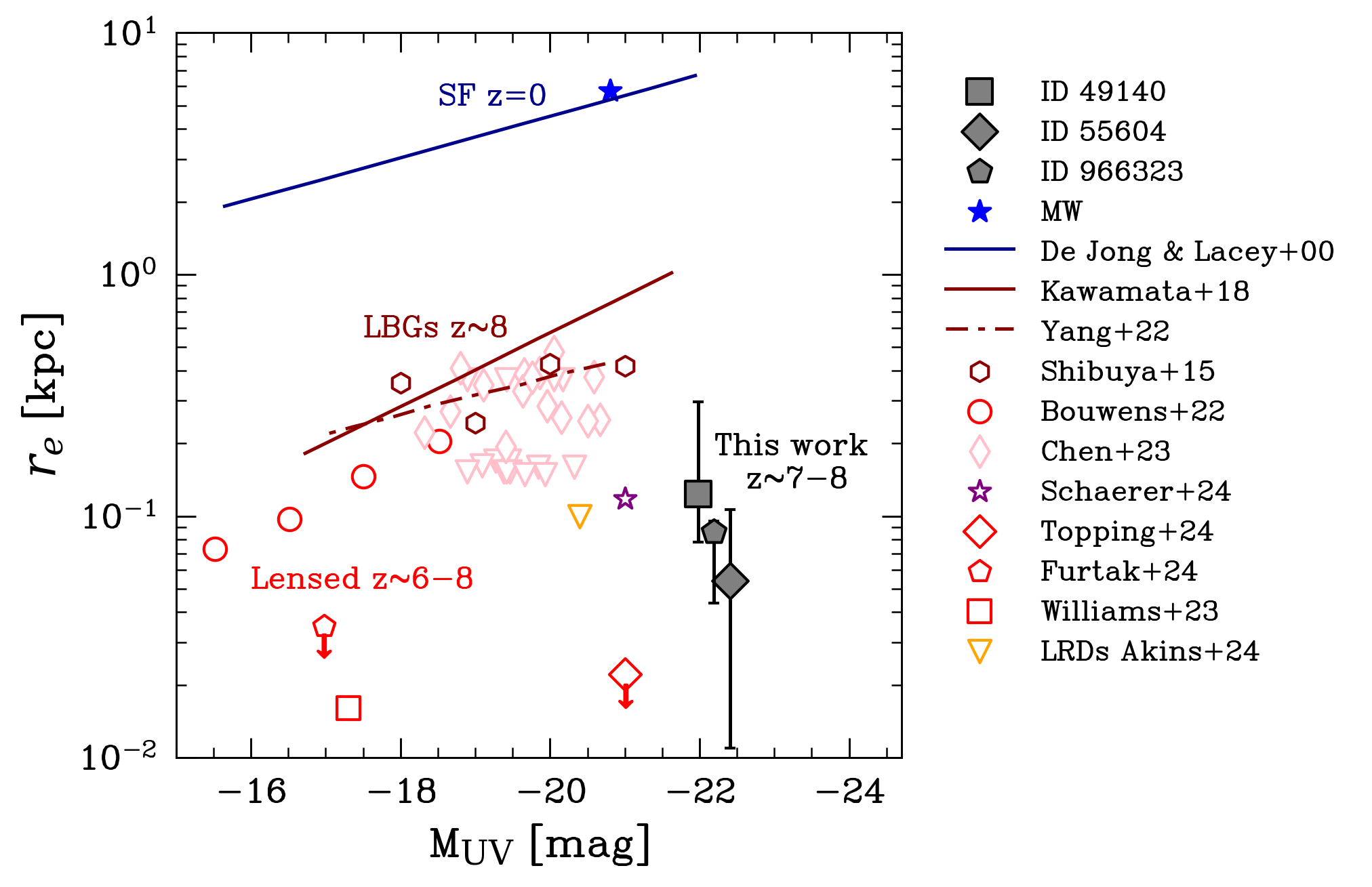
Figure 3: The size measured in F200W, plotted against the UV magnitude, measured from the spectrum at $\lambda_{\rm rest}$=150 nm. We also show size-luminosity derived for local spiral galaxies from de Jong & Lacey (2000) for which we use a magnitude correction $\rm M_{\rm UV}$-$\rm M_{\rm I}=1.0$, and LBGs at $z\sim 8$ (Shibuya et al., 2015; Bouwens et al., 2022; Kawamata et al., 2018), and $z\sim 9-12$ (Yang et al., 2022). In addition we show star-forming complexes (Chen et al., 2023) with $z_{\rm phot}\sim 6-8$. Finally, we show extremely compact sources, recently detected through lensing with JWST, reported in Furtak et al. (2024) ($R_{\rm e}<35$ pc, $z=7.0$), Topping et al. (2024) ($R_{\rm e}<22$ pc, $z=6.1$) and Williams et al. (2023) ($R_{\rm e}=16$ pc, $z=9.5$). Finally we show the upper limit of $\lesssim$100 pc reported for the brightest LRDs (Akins et al., 2024).

3.3 Sizes and Uncertainties

The masks, best-fitting models, and residuals from the fits are shown in Fig. 2. The fits are overall excellent. The effective radii are extremely small, $\sim$1.1 pixel or smaller. Using the spectroscopic redshifts of the galaxies, we find physical effective radii of 123 pc, 54 pc, and 86 pc for the three galaxies. To determine the uncertainties in these measurements we perform simulations to obtain upper and lower bounds for the sizes, taking into account the assumptions and unknowns in the modeling.

For each galaxy we consider a finely sampled array of possible sizes, from 0 to several pixels. For each test size $r_{\rm e,\,test}$ we simulate $10^{3}$ Sérsic models using galfit, with $r_{\rm e}=r_{\rm e,\,test}$ and the same integrated magnitude of the best fit model, while randomly assigning $b/a$ from 0.1 to 1, PA from 0 to 90 degrees, and $n$ from 0.5 to 6. We convolve these Sérsic models with either the stacked empirical PSF or WebbPSF. We then place these convolved models into the residual maps of the initial fits, so that differences between the galaxy profiles and Sérsic profiles are included in the errors. We fit these synthetic images following the same methodology as was used to fit the galaxies. This includes keeping $n=1.5$ fixed, fitting with WebbPSF, and solving for $r_{\mathrm{e}}$, $b/a$, the integrated magnitude, PA, and the sky background. This results in an array of $10^{3}$ different sizes for which the underlying model had a true size of $r_{\rm e,\,test}$. Next, we ask whether the observed size $r_{\rm e,\,obs}$ is within the central 68 % of the distribution of $10^{3}$ simulated sizes. If so, then $r_{\rm e,\,test}$ is deemed an acceptable true size of the object, and it is included in the $1\sigma$ errorbar for that galaxy.

We find that the uncertainties are asymmetric; with smaller true sizes being more likely than larger true sizes. This can be traced to two effects. First, our choice of the WebbPSF for the default measurement: convolving a galaxy with an empirical PSF and then fitting it with WebbPSF leads to a slight ($\sim 0.2$ pixel) overestimate of the size, and as half the simulations use empirical PSFs this leads to an overall bias in the simulated sizes. Second, there are more simulations with $n>1.5$ than with $n<1.5$, and fitting with fixed $n=1.5$ leads to a small (also $\sim 0.2$ pixels) bias.

A final uncertainty that has to be taken into account is our choice of fitting two galaxies (RUBIES-55604 and RUBIES-49140) with two components rather than one. We refit both galaxies with a single component to assess the importance of this choice. These fits lead to strong residuals, but they are stable. The half-light radii of both galaxies increase by a factor of $\sim$2 when they are fit as a single component. To account for this, we add the difference between the single-component and two-component fits in quadrature to the (positive) errorbars of these two galaxies. In Table 1 we report the measured sizes with their uncertainties.

3.4 Size-Luminosity Relation

The central observational result of this letter is the compactness of the three Balmer break galaxies at $z\sim 7-8$. The sizes for ID-55604 and ID-966323 are lower than measured in Baggen et al. (2023) for identical galaxies due to the new reduction scheme (see Section 2), but consistent within the errorbars. The average size of the three galaxies is $\langle r_{\rm e}\rangle\approx 90$ pc, smaller than the mean size of 150 pc in Baggen et al. (2023).

The sizes are similar to those of ultracompact dwarf galaxies ($r_{\mathrm{eff}}\leq$100 pc, e.g. Zhang et al., 2015), and smaller than any other moderately luminous galaxy population observed at $0<z<5$. To illustrate the extreme nature of these objects, we show the relation between effective radius (along the major axis) and UV magnitude ($\lambda_{\rm rest}\sim 1500$ Å) in Figure 3. Besides the three Balmer break galaxies we show the relation for local spiral galaxies, obtained from de Jong & Lacey (2000), for which we correct the measured $i$-band magnitudes to UV magnitude using $\rm M_{\rm UV}$-$\rm M_{\rm I}=1.0$, following Grazian et al. (2012). We also show the size-luminosity relation for Lyman-break-galaxies (LBGs) detected prior to JWST at $z\sim 8$ from Shibuya et al. (2015), Bouwens et al. (2022), Kawamata et al. (2018), as well as recently detected galaxies with JWST at $z\sim 9-12$ from Yang et al. (2022). At fixed absolute magnitude, these galaxies are about $100\times$ smaller than local spiral galaxies and about $10\times$ smaller than Lyman Break Galaxies (LBGs) at the same redshifts. Instead, their sizes are similar to those of lensed sources, reported in Bouwens et al. (2022), which are $\sim 6$ magnitudes fainter. However, these sizes corroborate with some of the most recent results with JWST. We show the sizes (diamond) and upper limits (triangle) of star-forming complexes reported in Chen et al. (2023) with $z_{\rm phot}\sim 6-8$. In addition, we show a bright compact galaxy at $z_{\rm spec}=9.4$ with $R_{\rm e}=118$ pc (Schaerer et al., 2024b). Extremely compact sources, recently detected through lensing with JWST, reported in Furtak et al. (2024) ($R_{\rm e}<35$ pc, $z=7.0$), Topping et al. (2024) ($R_{\rm e}<22$ pc, $z=6.1$), Williams et al. (2023) ($R_{\rm e}=16$ pc, $z=9.5$) are shown as red scatter points. Finally, we show the reported upper limits on effective radii of 434 LRDs from Akins et al. (2024). We show $r_{\rm e}\leq 100$ as a reference upper limit (for brightest LRDs) and use the UV magnitude of the observed stacked spectrum (at $\lambda_{\rm obs}=1.15\mu\rm m$, $F=15.76$ nJy, $M_{\rm UV}\sim-$20.4).

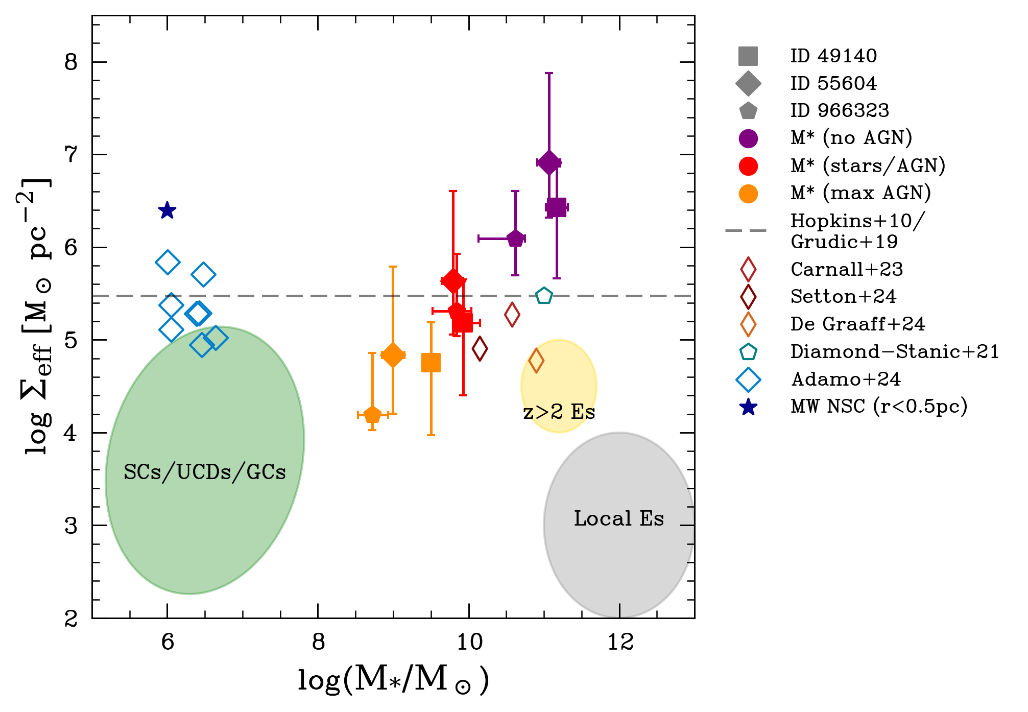
Figure 4: The surface density ($\Sigma_{\mathrm{eff}}=M_{*}(<R_{\mathrm{e}})/\pi R_{\mathrm{e}}^{2}$) plotted against stellar mass. We show a theoretical limit $\Sigma_{\mathrm{eff}}\leqq 3\times 10^{5}\mathrm{M}_{\odot}\mathrm{pc}^{-2}$, determined by Grudić et al. (2019) as the dashed black line. For illustration, we show regions in $M_{*}-\Sigma_{\mathrm{eff}}$ space for multiple stellar systems estimated from Hopkins et al. (2010), the class of star clusters (SC), ultracompact dwarf galaxies (UCD) and globular clusters (GCs) (green), local elliptical galaxies (grey) and compact $z>2$ elliptical galaxies (yellow). We also show (see text) quiescent galaxies at $z\sim 4-5$ (Setton et al., 2024; de Graaff et al., 2024; Carnall et al., 2023), compact starburst galaxies at $z\sim 2$ (Diamond-Stanic et al., 2021), Cosmic Gems star clusters at $z\sim 10$ (Adamo et al., 2024) and the MW nuclear star cluster. The surface density measured for the three Balmer break galaxies are shown for the three sets of stellar masses $M_{*,\mathrm{min}}$, $M_{*,\mathrm{med}}$ and $M_{*,\mathrm{max}}$ in orange, red and purple, respectively.

4 Densities and Kinematics

The small sizes, combined with the masses determined in Wang et al. (2024b), imply very high densities. Here we assess the average surface density of the galaxies (4.1), their 3D density profiles (4.2), and the expected kinematics (4.3). In each subsection we consider all three mass measurements of Wang et al. (2024b), for minimal, medium, and maximal AGN contributions, and indicate those with different colors in the figures.

4.1 Effective Surface Density

The average surface density within the effective radius can be calculated with

$$\Sigma_{\mathrm{eff}}=M_{*}(<R_{\mathrm{e}})/\pi R_{\mathrm{e}}^{2},$$ (1)

where $M_{*}(<R_{\mathrm{e}})=M_{*}/2$ and $R_{\mathrm{e}}$ is the projected circularized half-stellar mass radius $R_{\rm e}=r_{\mathrm{e,maj}}\sqrt{b/a}$ (ignoring $M/L$ gradients).

In Figure 4 we show the surface densities for the three galaxies, and for the three different stellar mass measurements of Wang et al. (2024b); $M_{*,\mathrm{min}}$, $M_{*,\mathrm{med}}$ and $M_{*,\mathrm{max}}$ in orange, red and purple, respectively. For context, we also show regions in $M_{*}-\Sigma_{\mathrm{eff}}$ space for various stellar systems, as estimated in Hopkins et al. (2010). Nuclear star clusters, ultracompact dwarf galaxies, dSph nuclei and globular clusters are taken together and shown in green, local elliptical galaxies are shown in grey, and compact $z>2$ elliptical galaxies are shown in yellow. We also show recently discovered star clusters at $z\sim 10$ (Adamo et al., 2024) in the Cosmic Gems arc.

In addition, we show the surface densities derived for three quiescent massive galaxies at $z=4-5$ from Carnall et al. (2023), Setton et al. (2024), de Graaff et al. (2024). For these quiescent galaxies the effective radii are circularized using $b/a$=0.7, when not reported, adopting the value reported for the compact component in Setton et al. (2024). Finally, we show the central surface densities for the compact starburst galaxies at $z\sim 2$ (Diamond-Stanic et al., 2021).

The black dashed line shows an effective surface stellar mass density of $\Sigma_{\mathrm{eff}}\leqq 3\times 10^{5}\mathrm{M}_{\odot}\mathrm{pc}^{-2}$. In the local Universe, very few stellar systems exceed this limit, going all the way from star clusters and globular clusters to elliptical galaxies (Hopkins et al., 2010; Grudić et al., 2019). It has been suggested that some universal mechanism controls the surface density: Hopkins et al. (2010) propose that feedback from massive stars in the form of winds and radiation fields is likely responsible for the observed $\Sigma_{\rm max}$. Grudić et al. (2019) propose an alternative model, relating the stellar feedback and star formation efficiency (SFE).

The surface densities of the three galaxies discussed here are extremely high. They are above the empirical surface density limit of Hopkins et al. (2010) by an order of magnitude in the no-AGN model, are on the limit for the mixed model, and are below the limit only for the maximal AGN model. The densities are also higher by several orders of magnitude than those of plausible descendants, elliptical galaxies at $z=0$.

The densities are most extreme for the no-AGN model, and this could be taken as evidence against it. However, we note that some nuclear star clusters reach $\sim 10^{6}\mathrm{M}_{\odot}\mathrm{pc}^{-2}$ in their centers, above the empirical limit. An important example is the nuclear star cluster in the center of the Milky Way around SgrA^∗, which reaches $2.5\times 10^{6}\,\mathrm{M}_{\odot}\mathrm{pc}^{-2}$ within the central 0.5 pc (see the review by Neumayer, 2017), indicated in Figure 4 as a dark blue star. We calculated this surface density using a stellar mass within this region of $M_{*}\sim 10^{6}\mathrm{M}_{\odot}$ (Schödel et al., 2009).

4.2 Stellar Mass Profiles

As first discussed in Bezanson et al. (2009), extreme densities within the effective radius do not necessarily correspond to extreme densities on small physical scales. The effective radius evolves, and if galaxies grow inside-out, their surface density within the effective radius goes down with time even if their density within a fixed small physical radius remains constant.

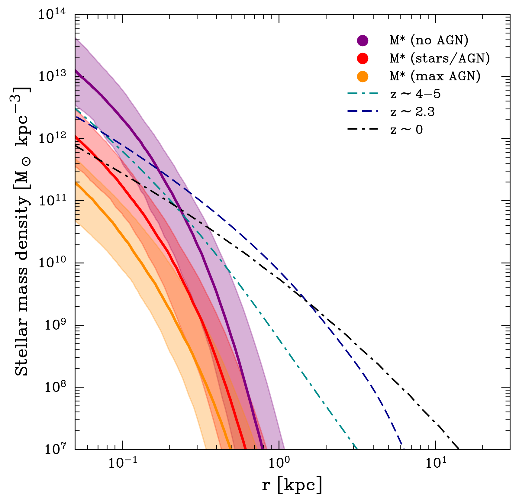
Figure 5: The median stellar mass profiles for the three sets of stellar masses (see Table 1), $M_{*,\mathrm{min}}$, $M_{*,\mathrm{med}}$ and $M_{*,\mathrm{max}}$ in orange, red and purple, respectively. We also show the stellar mass profiles of massive quiescent galaxies at different cosmic times: the mean stellar mass profile of three compact massive quiescent galaxies at $z\sim 4-5$ (Carnall et al., 2023; Setton et al., 2024; de Graaff et al., 2024), $z\sim 2.3$ compact elliptical galaxies (Bezanson et al., 2009), and massive elliptical galaxies at $z=0$ (Tal et al., 2009).

Following Baggen et al. (2023) we show the 3D density profiles of the galaxies in Fig. 5. The profiles were determined from the radii and the three different sets of stellar masses, using the same methodology as in Baggen et al. (2023). In short, we perform an Abel transform to the 2D best-fit Sérsic profile (see Table 1). After that, the luminosity profile is converted into a stellar mass profile by assuming the $M/L$ ratio does not change with radius. The profile is then scaled such that the total stellar masses are identical to those derived in Wang et al. (2024b). The uncertainty bands reflect the uncertainties in both the radii and the masses. We also show the stellar mass profiles of massive quiescent galaxies at different cosmic times: $z\sim 0$ elliptical galaxies (Tal et al., 2009), $z\sim 2.3$ compact elliptical galaxies from Bezanson et al. (2009), and the mean mass profile for three quiescent galaxies at $z\sim 4-5$ (Carnall et al., 2023; Setton et al., 2024; de Graaff et al., 2024).

We find that the central stellar mass densities are similar to those of plausible descendants for the medium mass model (red points), and that they are lower for the lowest masses (the maximal AGN model). Strikingly, the central densities are extremely high for the no-AGN masses (purple): $\sim 10^{13}$ M_⊙ kpc^-3 in the inner tens of pc, comparable to the densest nuclear star clusters (Pechetti et al., 2020). They are an order of magnitude above the density of plausible $z\sim 0$ descendants, and also higher (by a factor of $\sim 5$) than quiescent galaxies at $z=4-5$. If the no-AGN stellar masses are correct, it means that inside-out growth alone is not sufficient to connect these galaxies to their plausible descendants. The densities need to evolve downward, in order to be consistent with the central densities in the cores of quiescent galaxies at $z=0-5$. We return to this in § 5.

4.3 Kinematics

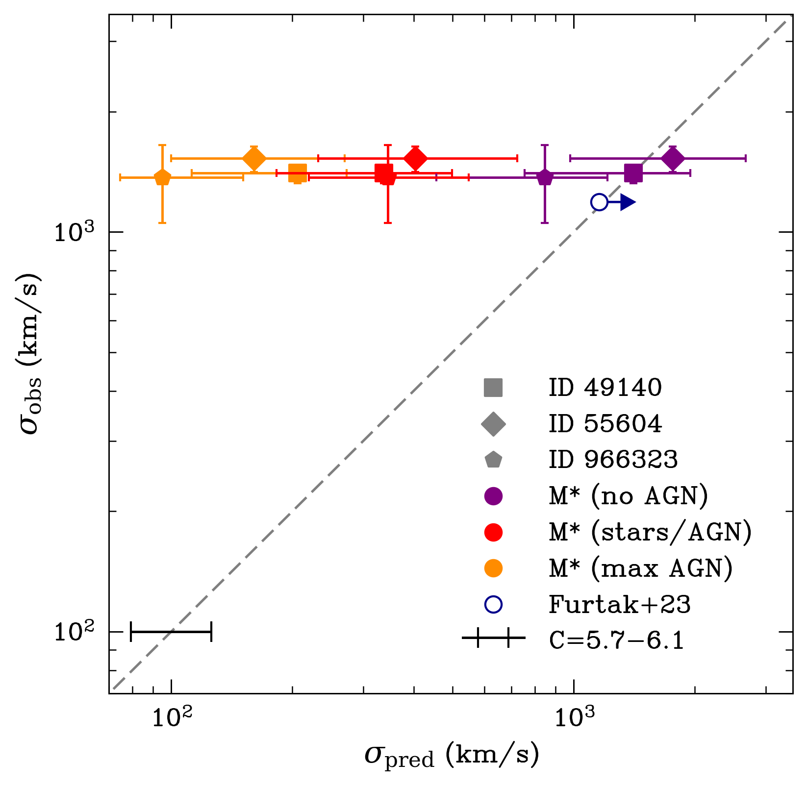
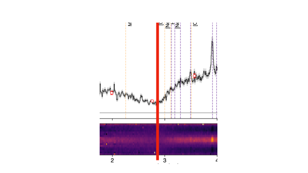
Figure 6: The observed velocity dispersion of the broad H$\beta$ lines plotted against the predicted velocity dispersion based on Eq. 3 using the measured effective radius and stellar masses (Table 1). We show the three stellar mass models, $M_{*,\mathrm{min}}$, $M_{*,\mathrm{med}}$ and $M_{*,\mathrm{max}}$ in orange, red and purple, respectively. We predict high velocity dispersions, up to a few hundred km s^-1 for the medium stellar mass scenario and $\sigma\gtrapprox$1000 km s^-1 for the maximum stellar mass scenario, similar to the observed velocities. The black errorbar in the lower left corner indicates how each measurement would shift horizontally when using different relations for Eq. 3, with $C=5.7$ (to the right) and $C=6.1$ (to the left). In the no-AGN model, the predicted velocity dispersions are very similar to the observed H$\beta$ line widths. Perhaps, the broad Balmer emission lines in these galaxies could simply be the result of the small sizes and high masses of the galaxies. The right figure shows a schematic view of this scenario.

From a simple virial equilibrium argument, we can relate the dynamical mass ($M_{\rm dyn}$) of a galaxy to its velocity dispersion $\sigma$ at radius $r$:

$$\sigma^{2}\approx\frac{GM_{\rm dyn}(<r)}{kr}.$$ (2)

for which the virial coefficient $k$, depends on the galaxy structure and the shape of the velocity dispersion profile, and is typically assumed to be between $\sim 3-5$ (e.g., Cappellari et al., 2006; Franx et al., 2008; Taylor et al., 2010; van der Wel et al., 2006) If we make assumptions about the properties of the stars and gas in the system, following e.g. van Dokkum et al. (2015), we can also relate the velocity dispersion of the gas, to the stellar mass and circularized effective radius:

$$\log(\sigma_{\mathrm{pred}})=0.5\left[\log(M_{*})-\log(r_{\mathrm{e}})-C\right],$$ (3)

where $\sigma_{\mathrm{pred}}$ in $\mathrm{km\,s^{-1}}$, $M_{*}$ in units of $\mathrm{M}_{\odot}$, and $r_{\mathrm{e}}$ in kpc. The constant $C$ is uncertain, as it depends on the inclination and dynamics of the gas and stars, on their mass contributions, and on their relative spatial distributions. Following van Dokkum et al. (2015) we adopt $C=5.9$, but to account for the uncertainties in the properties of the systems, we also consider the relations for $C=6.1$ (as used in Bezanson et al., 2009), which corresponds to $1.25\times$ lower expected velocity dispersions for a given mass and size, and $C=5.7$ ($1.25\times$ higher dispersions). For convenience, the full derivation along with all detailed assumptions is provided in Appendix A.

In Figure 6 we compare the expected velocity dispersion calculated with Eq. 3 to the measured widths of the H$\beta$ lines in the three galaxies. The errorbars reflect the uncertainties in size and mass. The black errorbar in the lower left corner indicates how each measurement would shift horizontally when using $C=5.7$ (to the right) and $C=6.1$ (to the left). The expected dispersions are a strong function of the choice of stellar mass, ranging from $\sim 150$ km s^-1 for the minimal masses to $\gtrsim 1000$ km s^-1 for the maximal (no-AGN) mass.

Remarkably, the expected dispersions are very similar to the observed H$\beta$ line widths for the no-AGN model. The implication is that the broad Balmer emission lines in these galaxies could simply be the result of the small sizes and high masses of the galaxies, rather than caused by the broad line regions around supermassive black holes. For reference, we also show the strongly-lensed red, compact source reported in Furtak et al. (2023, 2024), which has a superficially similar spectrum as the three Balmer break objects in the present study. The upper limit to the effective radius is $R_{\rm e}\leq 35$ pc, and the stellar mass for an SED dominated by stars is $\log(M_{*}/\mathrm{M}_{\odot})=10.57$ for this object. This gives an expected velocity dispersion (lower limit) similar to the reported value from the H$\beta$ line ($\sigma$ =FWHM/2.35 = 1190  km s^-1).

An important caveat is that the forbidden [O iii] lines in the three galaxies are narrow, of order $\sigma\sim 50-70$ km s^-1. In an AGN scenario this is explained by the high density of the gas close to the black hole: the forbidden lines cannot form there, because the collisional de-excitation rate exceeds the radiative de-excitation rate. Forbidden lines arise from a narrow line region (NLR) at larger distance. Interestingly, this same effect could be at work in the no-AGN scenario. We derive the density of the gas as follows. If we assume the gas and the stars follow the same spatial distribution, $r_{\rm gas}\sim r_{\rm stars}\sim r_{\rm e}$, the ratio of the scale height to the scale length is $c/a\sim 0.5$, and $M_{\rm gas}\sim 0.5M_{\rm stars}$, we obtain a gas density of $\rm N=10^{6.0}-10^{6.9}\rm\,cm^{-3}$, which is larger than the critical density for the forbidden line ($N_{\mathrm{cr,OIII,5007\AA}}=10^{5.8}\mathrm{cm}^{-3}$). If the gas disk is thinner (i.e., $c/a<0.5$) the gas is even denser.

5 Discussion

The main observational result of this Letter is a confirmation of the existence of extremely small ($r_{\rm e}\sim 100$ pc), luminous galaxies in the early Universe, at $z=6-8$. Unlike other high redshift galaxies, we know that the light at $\lambda_{\rm obs}=2\,\mu$m is dominated by stars, thanks to the detection of Balmer breaks in the spectra (Wang et al., 2024b). Despite the accurate sizes and the Balmer break detections, the densities of the galaxies remain uncertain, because AGN might contribute to the long wavelength flux (see Wang et al., 2024b).

We show that the maximal mass (that is, no AGN) models produce objects that are an order of magnitude denser in their centers than any other known galaxies. This might be taken as evidence against such models, except that they predict line widths that correspond remarkably well to the observed broad widths of the H$\beta$ lines. If this is the correct interpretation for these galaxies, it may apply to many other ‘little red dots’ with broad emission lines as well. It would provide a natural explanation for the lack of X-ray detections, lack of variability, and relatively faint MIRI fluxes of these galaxies (see the discussion and references in the Introduction).

It remains to be seen whether this scenario can explain all aspects of these systems. First, the high luminosity in H$\beta$ ($L>10^{42}$ erg s^-1) may require an exotic mechanism for photoionizing the gas. While AGNs are the most straightforward explanation, there are other possibilities. The extremely high density of the gas may lead to collisional excitation or shocks being a significant contributor (e.g. Davidson & Kinman, 1985; Draine & McKee, 1993; Stasińska & Izotov, 2001; Stasińska & Schaerer, 1999; Raga et al., 2015). There is also some evidence for the presence of very massive stars at high redshift (Upadhyaya et al., 2024), with higher ionizing power than typical stellar populations (e.g., Schaerer et al., 2024a). IMFs favoring the formation of massive stars can also explain the population of bright galaxies at $z>10$ (Harikane et al., 2023b; Inayoshi et al., 2022; Menon et al., 2024; Trinca et al., 2024; Yung et al., 2024). We note that alternative IMFs also change the stellar masses of the galaxies. In particular, recently van Dokkum & Conroy (2024) proposed a ’concordance IMF’, with a steep low mass slope and a shallow high mass slope. The shape of this IMF is capable of reconciling both the high redshift bright, massive galaxies, and observations of the cores of the most massive galaxies in the local Universe. This IMF produces slightly lower stellar masses for the three galaxies than the Kroupa (2001) IMF used by Wang et al. (2024b), but the change is much smaller than the effects of including AGNs in the modeling.

Second, the [O iii] lines should be spatially-extended with respect to the Balmer lines. The spatial sampling of the NIRSpec data ($0\farcs 06-0\farcs 1$) is, however, too coarse to confidently detect this effect in the current data, but high resolution observations (with the NIRCam grism, or of a lensed system) should show this differential effect. Third, the line profiles of the Balmer emission lines should not be perfectly Gaussian but reflect rotation (see, e.g., van Dokkum et al., 2015). There is some evidence for asymmetries and perhaps two peaks in the medium-resolution spectra of Wang et al. (2024b), but this could also be interpreted as absorption (see e.g. Wang et al., 2024a; Juodžbalis et al., 2024b). Finally, a stellar velocity dispersion measurement would be definitive. Such a case for an LRD has been reported very recently in Kokorev et al. (2024), a little red dot with a massive ($\log(M_{*}/\mathrm{M}_{\odot})\sim 10.6$) quenched galaxy host which is also compact ($r_{\rm e}\leq 300$ pc), for which a velocity dispersion of $\sigma\sim 400$km s^-1 is predicted, identical to the observed broad stellar absorption lines. There is a broad H$\beta$ absorption component, but it is too weak to robustly determine the width of the line. A further test for these Balmer break galaxies is that for $\sigma>1000$ km s^-1 the blended absorption lines in the Balmer break region take on a different shape than for “normal” velocity dispersions, and this should be detectable in high S/N spectra.

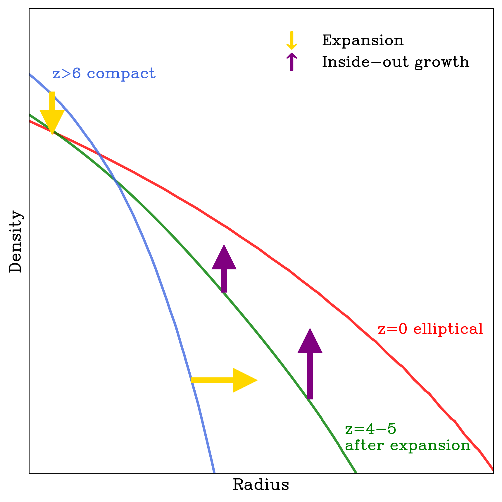
Figure 7: A possible pathway of the massive compact galaxies at $z>6$ in the no-AGN scenario. First, a phase of expansion as a result of mass loss (triggered by feedback e.g. Fan et al., 2008) or interaction of the SMBH with the stars in the central region (e.g. Begelman et al., 1980; Ebisuzaki et al., 1991; Hills, 1983; Quinlan, 1996) is required to lower the densities and velocity dispersions to those of massive compact quiescent galaxies at $z=4-5$. After that the galaxies grow mainly in an inside-out fashion, due to minor mergers (e.g. Naab et al., 2009; Bezanson et al., 2009; van Dokkum et al., 2010).

If this interpretation were confirmed, key questions are what might have caused such extremely dense galaxies to form, and how they evolve into “normal” systems with larger sizes and lower central densities. Perhaps the conditions in these systems are such that feedback free starbursts (FFB) can occur (Dekel et al., 2023), with the lack of feedback leading to extreme star formation efficiencies and thereby extreme stellar masses. FFB galaxies are indeed expected to be compact (Li et al., 2023). It was also recently suggested that the compactness may simply be driven by the steepness of dark matter profiles at $z=10-14$ (Boylan-Kolchin, 2024). Some general hydrodynamical simulations also produce small sizes for the most massive galaxies, such as $z\sim 6$ galaxies in TNG50 (Costantin et al., 2023) and $z\sim 7$ galaxies in the BLUETIDES simulation (Marshall et al., 2022). In addition, Roper et al. (2023) find that bulge formation begins by efficient cooling and high star formation rates in the cores down to effective radii of $r_{\rm e}\sim 100$ pc in the FLARES simulation. However, others find discrepancies between the observed and simulated sizes of high-redshift galaxies (e.g. THESAN, Shen et al., 2024). It remains an open question why compactness seems to be such a generic feature of early bright star-forming galaxies ($z\sim 7-9$, $r_{\rm e}\sim 100-300$ pc, e.g. Baggen et al., 2023; Akins et al., 2023; Langeroodi & Hjorth, 2023; Baker et al., 2023; Schaerer et al., 2024b; Ono et al., 2023) and massive quiescent galaxies out to $z\sim 5$ ($r_{\rm e}\sim 200-500$ pc, e.g. Ji et al., 2024; Wright et al., 2024; Setton et al., 2024; Carnall et al., 2023; de Graaff et al., 2024; Kokorev et al., 2024).

Whatever the formation mechanism, in the no-AGN scenario, dramatic evolution is required to bring the stellar mass densities in line with those of plausible descendants. One possible mechanism is adiabatic expansion due to feedback-driven mass loss, from AGNs or stellar winds (Fan et al., 2008). Feedback may be suppressed at early times (Dekel et al., 2023) and then become very effective once it is “turned on”. Another mechanism is scouring by a binary SMBH (e.g. Begelman et al., 1980; Ebisuzaki et al., 1991; Hills, 1983; Quinlan, 1996), after a merger. The ejection of stars from the core lowers the density, increases the size, and likely also reduces rotational support (e.g., Rantala et al., 2024). While these models have been proposed to explain the size evolution of lower redshift ($z\sim 2$) compact red nuggets, as well as the formation of cores in present-day ellipticals, they work on the right spatial scales to be relevant here. An attractive feature of such scenarios is that they act quickly, lower the central density and increase the effective radius, and keep the stellar mass roughly constant, bringing the galaxies close to observed quiescent galaxies at $z=4-5$ (Setton et al., 2024; Carnall et al., 2023; de Graaff et al., 2024). After this expansion phase the galaxies slowly grow inside-out, largely due to minor mergers (see, e.g., Naab et al., 2009; van Dokkum et al., 2010). These pathways are illustrated in Figure 7.

It also remains to be seen whether these ultra compact galaxies are stable against gravitational collapse; it may that parts of the galaxies collapse into supermassive black holes while the rest expands (Lynden-Bell & Wood (1968), and see also Dekel et al. in prep).

Finally, we stress that the standard interpretation of the broad Balmer emission lines, namely broad line regions around supermassive black holes, remains viable — and perhaps more likely. Future observations may show whether the continuum is dominated by AGN light or stellar light, for instance through probing the red continuum beyond $\lambda_{\rm rest}=1.6\,\mu$m with ALMA/MIRI (see, e.g., Akins et al., 2024; Labbé et al., 2023b; Iani et al., 2024; Pérez-González et al., 2024; Williams et al., 2024). The no-AGN solution that we explore here is self-consistent and intriguing, but it requires further evidence.

Appendix A Expected velocity dispersion

In this appendix, we show the derivation of Eq. 3, following van Dokkum et al. (2015) and references therein.

The observed velocity dispersion of the gas, which is the second moment of the velocity distribution of the gas along the line of sight, for an unresolved rotating disk is given by:

$$\sigma^{2}_{\rm gas}=\alpha^{2}V_{\rm rot}^{2}\sin^{2}{i}+\sigma_{\rm random}^{2},$$ (A1)

where $i$ is the inclination (such that face-on systems have $i=0$ and edge-on disks have $i=90$), $\alpha$ is typically $\sim 0.6-1$ (Franx, 1993; Rix et al., 1997; Weiner et al., 2006). The random motion term contains the dispersions within the gas clouds in the ISM and inclination dependent non-gravitational motions such as winds: $\sigma_{\rm random}^{2}=\sigma^{2}_{\rm ism}+w^{2}(i)\sigma^{2}_{\rm wind}$. The rotation velocity ($V_{\rm rot}$) of the gas at a radius $r_{\rm gas}$ is related via the virial theorem to the dynamical mass enclosed in $r_{\rm gas}$:

$$V_{\rm rot,gas}^{2}=\frac{GM_{\rm dyn}(<r_{\rm gas})}{k\,r_{\rm gas}},$$ (A2)

where $k$ is the (typically radius-dependent) virial coefficient. For a perfectly spherical case, $k=1$, but for a thin disk, a value of $k=1.8$ (corresponding to $n=1$) is typically used (see e.g. Rowland et al., 2024). We assume that the stars in the compact galaxies in this work formed simultaneously with the gas, such that they have the same distribution and kinematics. Therefore, we assume that the size of the gas disk is equal to that of the stars, $r_{\mathrm{gas}}=r_{\mathrm{stars}}=r_{\mathrm{e}}$. In principle, this might not be true at all (see discussion in van Dokkum et al., 2015); the gas could either be more extended, or more compact. If we also ignore the random motions of the gas, we obtain:

$$\sigma^{2}_{\rm gas}=\alpha^{2}\sin^{2}{(i)}\frac{GM_{\rm dyn}(<r_{\rm e})}{kr_{\rm e}}$$ (A3)

Assuming that the dynamical mass consists of gas and stars, neglecting dark matter in the center, we have $M_{\rm dyn}(<r_{\rm e})=M_{\rm gas}(<r_{\rm e})+M_{\rm*}(<r_{\rm e})$. If we then assume the mass fraction in gas and stars to be equal ($f_{\rm gas}=0.5$), we have $M_{\rm dyn}(<r_{\rm e})=2M_{\rm*}(<r_{\rm e})$, where the half light radius contains half the stellar mass so $M_{\rm dyn}(<r_{\rm e})=M_{*}$. Plugging in numbers for $\alpha\sim 0.8$, $k=1$, $i=45^{\circ}$ and $G=4.3\times 10^{-6}$ if $\sigma$ in km s^-1, $M_{\rm dyn}$ in units of $\mathrm{M}_{\odot}$, $r_{\mathrm{e}}$ in kpc, we have the expected velocity dispersion of the gas, as a function of stellar mass and effective radius:

$$\log\sigma_{\rm pred}=0.5\left[\log(M_{*})-\log(r_{\rm e})-5.9\right].$$ (A4)

It is clear that the constant $C$ can vary, depending on the assumed properties of the system. For example, if we assume $k=1.8$ instead of $k=1$, we get $C=6.1$ (x1.25 lower velocity dispersion), while an inclination of $i=60^{\circ}$ would lead to $C=5.7$ (x1.25 higher velocity dispersion).

References

- Adamo et al. (2024) Adamo, A., Bradley, L. D., Vanzella, E., et al. 2024, arXiv e-prints, arXiv:2401.03224, doi: 10.48550/arXiv.2401.03224
- Akins et al. (2023) Akins, H. B., Casey, C. M., Allen, N., et al. 2023, ApJ, 956, 61, doi: 10.3847/1538-4357/acef21
- Akins et al. (2024) Akins, H. B., Casey, C. M., Lambrides, E., et al. 2024, arXiv e-prints, arXiv:2406.10341, doi: 10.48550/arXiv.2406.10341
- Ananna et al. (2024) Ananna, T. T., Bogdán, Á., Kovács, O. E., Natarajan, P., & Hickox, R. C. 2024, ApJ, 969, L18, doi: 10.3847/2041-8213/ad5669
- Baggen et al. (2023) Baggen, J. F. W., van Dokkum, P., Labbé, I., et al. 2023, ApJ, 955, L12, doi: 10.3847/2041-8213/acf5ef
- Baker et al. (2023) Baker, W. M., Tacchella, S., Johnson, B. D., et al. 2023, arXiv e-prints, arXiv:2306.02472, doi: 10.48550/arXiv.2306.02472
- Balogh et al. (1999) Balogh, M. L., Morris, S. L., Yee, H. K. C., Carlberg, R. G., & Ellingson, E. 1999, ApJ, 527, 54, doi: 10.1086/308056
- Barro et al. (2024) Barro, G., Pérez-González, P. G., Kocevski, D. D., et al. 2024, ApJ, 963, 128, doi: 10.3847/1538-4357/ad167e
- Begelman et al. (1980) Begelman, M. C., Blandford, R. D., & Rees, M. J. 1980, Nature, 287, 307, doi: 10.1038/287307a0
- Bezanson et al. (2009) Bezanson, R., van Dokkum, P. G., Tal, T., et al. 2009, ApJ, 697, 1290, doi: 10.1088/0004-637X/697/2/1290
- Bogdán et al. (2024) Bogdán, Á., Goulding, A. D., Natarajan, P., et al. 2024, Nature Astronomy, 8, 126, doi: 10.1038/s41550-023-02111-9
- Bouwens et al. (2022) Bouwens, R. J., Illingworth, G. D., van Dokkum, P. G., et al. 2022, ApJ, 927, 81, doi: 10.3847/1538-4357/ac4791
- Boylan-Kolchin (2023) Boylan-Kolchin, M. 2023, Nature Astronomy, 7, 731, doi: 10.1038/s41550-023-01937-7
- Boylan-Kolchin (2024) —. 2024, arXiv e-prints, arXiv:2407.10900. https://arxiv.org/abs/2407.10900
- Brammer (2023) Brammer, G. 2023, grizli, 1.5.2, Zenodo, doi: 10.5281/ZENODO.1146904
- Bruzual A. (1983) Bruzual A., G. 1983, ApJ, 273, 105, doi: 10.1086/161352
- Cappellari et al. (2006) Cappellari, M., Bacon, R., Bureau, M., et al. 2006, MNRAS, 366, 1126, doi: 10.1111/j.1365-2966.2005.09981.x
- Carnall et al. (2023) Carnall, A. C., McLure, R. J., Dunlop, J. S., et al. 2023, Nature, 619, 716, doi: 10.1038/s41586-023-06158-6
- Chen et al. (2023) Chen, Z., Stark, D. P., Endsley, R., et al. 2023, MNRAS, 518, 5607, doi: 10.1093/mnras/stac3476
- Costantin et al. (2023) Costantin, L., Pérez-González, P. G., Vega-Ferrero, J., et al. 2023, ApJ, 946, 71, doi: 10.3847/1538-4357/acb926
- Davidson & Kinman (1985) Davidson, K., & Kinman, T. D. 1985, ApJS, 58, 321, doi: 10.1086/191044
- de Graaff et al. (2024) de Graaff, A., Setton, D. J., Brammer, G., et al. 2024, arXiv e-prints, arXiv:2404.05683, doi: 10.48550/arXiv.2404.05683
- de Jong & Lacey (2000) de Jong, R. S., & Lacey, C. 2000, ApJ, 545, 781, doi: 10.1086/317840
- Dekel et al. (2023) Dekel, A., Sarkar, K. C., Birnboim, Y., Mandelker, N., & Li, Z. 2023, MNRAS, 523, 3201, doi: 10.1093/mnras/stad1557
- Diamond-Stanic et al. (2021) Diamond-Stanic, A. M., Moustakas, J., Sell, P. H., et al. 2021, ApJ, 912, 11, doi: 10.3847/1538-4357/abe935
- Ding et al. (2022) Ding, X., Silverman, J. D., & Onoue, M. 2022, ApJ, 939, L28, doi: 10.3847/2041-8213/ac9c02
- Draine & McKee (1993) Draine, B. T., & McKee, C. F. 1993, ARA&A, 31, 373, doi: 10.1146/annurev.aa.31.090193.002105
- Ebisuzaki et al. (1991) Ebisuzaki, T., Makino, J., & Okumura, S. K. 1991, Nature, 354, 212, doi: 10.1038/354212a0
- Fan et al. (2008) Fan, L., Lapi, A., De Zotti, G., & Danese, L. 2008, ApJ, 689, L101, doi: 10.1086/595784
- Finkelstein et al. (2023a) Finkelstein, S. L., Bagley, M. B., & Yang, G. 2023a, Data from The Cosmic Evolution Early Release Science Survey (CEERS), STScI/MAST, doi: 10.17909/Z7P0-8481
- Finkelstein et al. (2022) Finkelstein, S. L., Bagley, M. B., Haro, P. A., et al. 2022, ApJ, 940, L55, doi: 10.3847/2041-8213/ac966e
- Finkelstein et al. (2023b) Finkelstein, S. L., Bagley, M. B., Ferguson, H. C., et al. 2023b, ApJ, 946, L13, doi: 10.3847/2041-8213/acade4
- Franx (1993) Franx, M. 1993, in IAU Symposium, Vol. 153, Galactic Bulges, ed. H. Dejonghe & H. J. Habing, 243
- Franx et al. (2008) Franx, M., van Dokkum, P. G., Förster Schreiber, N. M., et al. 2008, ApJ, 688, 770, doi: 10.1086/592431
- Furtak et al. (2023) Furtak, L. J., Zitrin, A., Plat, A., et al. 2023, ApJ, 952, 142, doi: 10.3847/1538-4357/acdc9d
- Furtak et al. (2024) Furtak, L. J., Labbé, I., Zitrin, A., et al. 2024, Nature, 628, 57, doi: 10.1038/s41586-024-07184-8
- Grazian et al. (2012) Grazian, A., Castellano, M., Fontana, A., et al. 2012, A&A, 547, A51, doi: 10.1051/0004-6361/201219669
- Greene et al. (2024) Greene, J. E., Labbe, I., Goulding, A. D., et al. 2024, ApJ, 964, 39, doi: 10.3847/1538-4357/ad1e5f
- Grudić et al. (2019) Grudić, M. Y., Hopkins, P. F., Quataert, E., & Murray, N. 2019, MNRAS, 483, 5548, doi: 10.1093/mnras/sty3386
- Hamilton (1985) Hamilton, D. 1985, ApJ, 297, 371, doi: 10.1086/163537
- Harikane et al. (2023a) Harikane, Y., Zhang, Y., Nakajima, K., et al. 2023a, ApJ, 959, 39, doi: 10.3847/1538-4357/ad029e
- Harikane et al. (2023b) Harikane, Y., Ouchi, M., Oguri, M., et al. 2023b, ApJS, 265, 5, doi: 10.3847/1538-4365/acaaa9
- Heintz et al. (2024) Heintz, K. E., Brammer, G. B., Watson, D., et al. 2024, arXiv e-prints, arXiv:2404.02211, doi: 10.48550/arXiv.2404.02211
- Hills (1983) Hills, J. G. 1983, AJ, 88, 1269, doi: 10.1086/113418
- Hopkins et al. (2010) Hopkins, P. F., Murray, N., Quataert, E., & Thompson, T. A. 2010, MNRAS, 401, L19, doi: 10.1111/j.1745-3933.2009.00777.x
- Iani et al. (2024) Iani, E., Rinaldi, P., Caputi, K. I., et al. 2024, arXiv e-prints, arXiv:2406.18207, doi: 10.48550/arXiv.2406.18207
- Inayoshi et al. (2022) Inayoshi, K., Harikane, Y., Inoue, A. K., Li, W., & Ho, L. C. 2022, ApJ, 938, L10, doi: 10.3847/2041-8213/ac9310
- Inayoshi & Ichikawa (2024) Inayoshi, K., & Ichikawa, K. 2024, arXiv e-prints, arXiv:2402.14706, doi: 10.48550/arXiv.2402.14706
- Ji et al. (2024) Ji, Z., Williams, C. C., Suess, K. A., et al. 2024, arXiv e-prints, arXiv:2401.00934, doi: 10.48550/arXiv.2401.00934
- Juodžbalis et al. (2024a) Juodžbalis, I., Maiolino, R., Baker, W. M., et al. 2024a, arXiv e-prints, arXiv:2403.03872, doi: 10.48550/arXiv.2403.03872
- Juodžbalis et al. (2024b) Juodžbalis, I., Ji, X., Maiolino, R., et al. 2024b, arXiv e-prints, arXiv:2407.08643, doi: 10.48550/arXiv.2407.08643
- Kawamata et al. (2018) Kawamata, R., Ishigaki, M., Shimasaku, K., et al. 2018, ApJ, 855, 4, doi: 10.3847/1538-4357/aaa6cf
- Killi et al. (2023) Killi, M., Watson, D., Brammer, G., et al. 2023, arXiv e-prints, arXiv:2312.03065, doi: 10.48550/arXiv.2312.03065
- Kocevski et al. (2023) Kocevski, D. D., Onoue, M., Inayoshi, K., et al. 2023, arXiv e-prints, arXiv:2302.00012, doi: 10.48550/arXiv.2302.00012
- Kokorev et al. (2023) Kokorev, V., Fujimoto, S., Labbe, I., et al. 2023, ApJ, 957, L7, doi: 10.3847/2041-8213/ad037a
- Kokorev et al. (2024) Kokorev, V., Chisholm, J., Endsley, R., et al. 2024, arXiv e-prints, arXiv:2407.20320, doi: 10.48550/arXiv.2407.20320
- Kokubo & Harikane (2024) Kokubo, M., & Harikane, Y. 2024, arXiv e-prints, arXiv:2407.04777. https://arxiv.org/abs/2407.04777
- Kovács et al. (2024) Kovács, O. E., Bogdán, Á., Natarajan, P., et al. 2024, ApJ, 965, L21, doi: 10.3847/2041-8213/ad391f
- Labbé et al. (2023a) Labbé, I., van Dokkum, P., Nelson, E., et al. 2023a, Nature, 616, 266, doi: 10.1038/s41586-023-05786-2
- Labbé et al. (2023b) Labbé, I., Greene, J. E., Bezanson, R., et al. 2023b, arXiv e-prints, arXiv:2306.07320, doi: 10.48550/arXiv.2306.07320
- Langeroodi & Hjorth (2023) Langeroodi, D., & Hjorth, J. 2023, arXiv e-prints, arXiv:2307.06336, doi: 10.48550/arXiv.2307.06336
- Larson et al. (2023) Larson, R. L., Finkelstein, S. L., Kocevski, D. D., et al. 2023, ApJ, 953, L29, doi: 10.3847/2041-8213/ace619
- Li et al. (2023) Li, Z., Dekel, A., Sarkar, K. C., et al. 2023, arXiv e-prints, arXiv:2311.14662, doi: 10.48550/arXiv.2311.14662
- Lynden-Bell & Wood (1968) Lynden-Bell, D., & Wood, R. 1968, MNRAS, 138, 495, doi: 10.1093/mnras/138.4.495
- Maiolino et al. (2023) Maiolino, R., Scholtz, J., Curtis-Lake, E., et al. 2023, arXiv e-prints, arXiv:2308.01230, doi: 10.48550/arXiv.2308.01230
- Maiolino et al. (2024) Maiolino, R., Risaliti, G., Signorini, M., et al. 2024, arXiv e-prints, arXiv:2405.00504, doi: 10.48550/arXiv.2405.00504
- Marshall et al. (2022) Marshall, M. A., Wilkins, S., Di Matteo, T., et al. 2022, MNRAS, 511, 5475, doi: 10.1093/mnras/stac380
- Matthee et al. (2024) Matthee, J., Naidu, R. P., Brammer, G., et al. 2024, ApJ, 963, 129, doi: 10.3847/1538-4357/ad2345
- Menon et al. (2024) Menon, S. H., Lancaster, L., Burkhart, B., et al. 2024, ApJ, 967, L28, doi: 10.3847/2041-8213/ad462d
- Naab et al. (2009) Naab, T., Johansson, P. H., & Ostriker, J. P. 2009, ApJ, 699, L178, doi: 10.1088/0004-637X/699/2/L178
- Neumayer (2017) Neumayer, N. 2017, in Formation, Evolution, and Survival of Massive Star Clusters, ed. C. Charbonnel & A. Nota, Vol. 316, 84–90, doi: 10.1017/S1743921316007018
- Ono et al. (2023) Ono, Y., Harikane, Y., Ouchi, M., et al. 2023, ApJ, 951, 72, doi: 10.3847/1538-4357/acd44a
- Onoue et al. (2023) Onoue, M., Inayoshi, K., Ding, X., et al. 2023, ApJ, 942, L17, doi: 10.3847/2041-8213/aca9d3
- Pechetti et al. (2020) Pechetti, R., Seth, A., Neumayer, N., et al. 2020, ApJ, 900, 32, doi: 10.3847/1538-4357/abaaa7
- Peng et al. (2002) Peng, C. Y., Ho, L. C., Impey, C. D., & Rix, H.-W. 2002, AJ, 124, 266, doi: 10.1086/340952
- Peng et al. (2010) —. 2010, AJ, 139, 2097, doi: 10.1088/0004-6256/139/6/2097
- Pérez-González et al. (2024) Pérez-González, P. G., Barro, G., Rieke, G. H., et al. 2024, ApJ, 968, 4, doi: 10.3847/1538-4357/ad38bb
- Perrin et al. (2014) Perrin, M. D., Sivaramakrishnan, A., Lajoie, C.-P., et al. 2014, Proc SPIE, 9143, 91433X, doi: 10.1117/12.2056689
- Poggianti et al. (1999) Poggianti, B. M., Smail, I., Dressler, A., et al. 1999, ApJ, 518, 576, doi: 10.1086/307322
- Quinlan (1996) Quinlan, G. D. 1996, arXiv e-prints, astro, doi: 10.48550/arXiv.astro-ph/9601092
- Raga et al. (2015) Raga, A. C., Castellanos-Ramírez, A., Esquivel, A., Rodríguez-González, A., & Velázquez, P. F. 2015, Rev. Mexicana Astron. Astrofis., 51, 231
- Rantala et al. (2024) Rantala, A., Rawlings, A., Naab, T., Thomas, J., & Johansson, P. H. 2024, arXiv e-prints, arXiv:2407.18303, doi: 10.48550/arXiv.2407.18303
- Rix et al. (1997) Rix, H. W., Guhathakurta, P., Colless, M., & Ing, K. 1997, Mon. Not. Roy. Astron. Soc., 285, 779, doi: 10.1093/mnras/285.4.779
- Roper et al. (2023) Roper, W. J., Lovell, C. C., Vijayan, A. P., et al. 2023, MNRAS, 526, 6128, doi: 10.1093/mnras/stad2746
- Rowland et al. (2024) Rowland, L. E., Hodge, J., Bouwens, R., et al. 2024, arXiv e-prints, arXiv:2405.06025, doi: 10.48550/arXiv.2405.06025
- Schaerer et al. (2024a) Schaerer, D., Guibert, J., Marques-Chaves, R., & Martins, F. 2024a, arXiv e-prints, arXiv:2407.12122, doi: 10.48550/arXiv.2407.12122
- Schaerer et al. (2024b) Schaerer, D., Marques-Chaves, R., Xiao, M., & Korber, D. 2024b, A&A, 687, L11, doi: 10.1051/0004-6361/202450721
- Schödel et al. (2009) Schödel, R., Merritt, D., & Eckart, A. 2009, A&A, 502, 91, doi: 10.1051/0004-6361/200810922
- Sersic (1968) Sersic, J. L. 1968, Atlas de Galaxias Australes
- Setton et al. (2024) Setton, D. J., Khullar, G., Miller, T. B., et al. 2024, arXiv e-prints, arXiv:2402.05664, doi: 10.48550/arXiv.2402.05664
- Shen et al. (2024) Shen, X., Vogelsberger, M., Borrow, J., et al. 2024, arXiv e-prints, arXiv:2402.08717, doi: 10.48550/arXiv.2402.08717
- Shibuya et al. (2015) Shibuya, T., Ouchi, M., & Harikane, Y. 2015, ApJS, 219, 15, doi: 10.1088/0067-0049/219/2/15
- Silk et al. (2024) Silk, J., Begelman, M. C., Norman, C., Nusser, A., & Wyse, R. F. G. 2024, ApJ, 961, L39, doi: 10.3847/2041-8213/ad1bf0
- Stasińska & Izotov (2001) Stasińska, G., & Izotov, Y. 2001, A&A, 378, 817, doi: 10.1051/0004-6361:20011303
- Stasińska & Schaerer (1999) Stasińska, G., & Schaerer, D. 1999, A&A, 351, 72, doi: 10.48550/arXiv.astro-ph/9909203
- Tal et al. (2009) Tal, T., van Dokkum, P. G., Nelan, J., & Bezanson, R. 2009, AJ, 138, 1417, doi: 10.1088/0004-6256/138/5/1417
- Taylor et al. (2010) Taylor, E. N., Franx, M., Brinchmann, J., van der Wel, A., & van Dokkum, P. G. 2010, ApJ, 722, 1, doi: 10.1088/0004-637X/722/1/1
- Topping et al. (2024) Topping, M. W., Stark, D. P., Senchyna, P., et al. 2024, MNRAS, 529, 3301, doi: 10.1093/mnras/stae682
- Trinca et al. (2024) Trinca, A., Schneider, R., Valiante, R., et al. 2024, MNRAS, 529, 3563, doi: 10.1093/mnras/stae651
- Übler et al. (2023) Übler, H., Maiolino, R., Curtis-Lake, E., et al. 2023, A&A, 677, A145, doi: 10.1051/0004-6361/202346137
- Upadhyaya et al. (2024) Upadhyaya, A., Marques-Chaves, R., Schaerer, D., et al. 2024, A&A, 686, A185, doi: 10.1051/0004-6361/202449184
- van der Wel et al. (2006) van der Wel, A., Franx, M., Wuyts, S., et al. 2006, ApJ, 652, 97, doi: 10.1086/508128
- van Dokkum & Conroy (2024) van Dokkum, P., & Conroy, C. 2024, arXiv e-prints, arXiv:2407.06281, doi: 10.48550/arXiv.2407.06281
- van Dokkum et al. (2010) van Dokkum, P. G., Whitaker, K. E., Brammer, G., et al. 2010, ApJ, 709, 1018, doi: 10.1088/0004-637X/709/2/1018
- van Dokkum et al. (2015) van Dokkum, P. G., Nelson, E. J., Franx, M., et al. 2015, ApJ, 813, 23, doi: 10.1088/0004-637X/813/1/23
- Wang et al. (2024a) Wang, B., de Graaff, A., Davies, R. L., et al. 2024a, arXiv e-prints, arXiv:2403.02304, doi: 10.48550/arXiv.2403.02304
- Wang et al. (2024b) Wang, B., Leja, J., de Graaff, A., et al. 2024b, ApJ, 969, L13, doi: 10.3847/2041-8213/ad55f7
- Weaver et al. (2023) Weaver, J. R., Cutler, S. E., Pan, R., et al. 2023, arXiv e-prints, arXiv:2301.02671, doi: 10.48550/arXiv.2301.02671
- Weibel et al. (2024) Weibel, A., Oesch, P. A., Barrufet, L., et al. 2024, arXiv e-prints, arXiv:2403.08872, doi: 10.48550/arXiv.2403.08872
- Weiner et al. (2006) Weiner, B. J., Willmer, C. N. A., Faber, S. M., et al. 2006, ApJ, 653, 1027, doi: 10.1086/508921
- Williams et al. (2024) Williams, C. C., Alberts, S., Ji, Z., et al. 2024, ApJ, 968, 34, doi: 10.3847/1538-4357/ad3f17
- Williams et al. (2023) Williams, H., Kelly, P. L., Chen, W., et al. 2023, Science, 380, 416, doi: 10.1126/science.adf5307
- Worthey et al. (1994) Worthey, G., Faber, S. M., Gonzalez, J. J., & Burstein, D. 1994, ApJS, 94, 687, doi: 10.1086/192087
- Wright et al. (2024) Wright, L., Whitaker, K. E., Weaver, J. R., et al. 2024, ApJ, 964, L10, doi: 10.3847/2041-8213/ad2b6d
- Yang et al. (2022) Yang, L., Morishita, T., Leethochawalit, N., et al. 2022, ApJ, 938, L17, doi: 10.3847/2041-8213/ac8803
- Yue et al. (2024) Yue, M., Eilers, A.-C., Ananna, T. T., et al. 2024, arXiv e-prints, arXiv:2404.13290, doi: 10.48550/arXiv.2404.13290
- Yung et al. (2024) Yung, L. Y. A., Somerville, R. S., Finkelstein, S. L., Wilkins, S. M., & Gardner, J. P. 2024, MNRAS, 527, 5929, doi: 10.1093/mnras/stad3484
- Zhang et al. (2015) Zhang, H.-X., Peng, E. W., Côté, P., et al. 2015, ApJ, 802, 30, doi: 10.1088/0004-637X/802/1/30