Quantum Rational Transformation Using Linear Combinations of Hamiltonian Simulations

Abstract

Rational functions are exceptionally powerful tools in scientific computing, yet their abilities to advance quantum algorithms remain largely untapped. In this paper, we introduce effective implementations of rational transformations of a target operator on quantum hardware. By leveraging suitable integral representations of the operator resolvent, we show that rational transformations can be performed efficiently with Hamiltonian simulations using a linear-combination-of-unitaries (LCU). We formulate two complementary LCU approaches, discrete-time and continuous-time LCU, each providing unique strategies to decomposing the exact integral representations of a resolvent. We consider quantum rational transformation for the ubiquitous task of approximating functions of a Hermitian operator, with particular emphasis on the elementary signum function. For illustration, we discuss its application to the ground and excited state problems. Combining rational transformations with observable dynamic mode decomposition (ODMD), our recently developed noise-resilient quantum eigensolver, we design a fully real-time approach for resolving many-body spectra. Our numerical demonstration on spin systems indicates that our real-time framework is compact and achieves accurate estimation of the low-lying energies.

1 Introduction

Quantum algorithms for approximating functions of Hermitian operators have attracted theoretical and practical interest across domains of quantum information science and, among others, have been explored for computing eigenenergies, simulating quantum systems, and implementing quantum walks [27, 26, 46, 33, 34, 9, 6]. For many-body physics, localized functions with sufficiently tight support are instrumental in extracting essential spectral information, such as specific ground and excited state properties [37, 25]. In quantum linear algebra, elementary functions including the inverse, absolute value, and square root are intimately tied to common operator factorizations that find numerous applications. Most notably, the signum function can be employed to obtain the symmetric eigendecomposition and singular value decomposition of a matrix [38]. Often a function cannot be compiled exactly: in such cases it is extremely advantageous to employ a subset of simpler but expressive transformations to approximate a broader set of target functions.

Function approximation via polynomial transformations are enabled by approaches such as quantum signal processing (QSP), the quantum singular value transformation (QSVT), and the quantum eigenvalue transformation (QET) [33, 34, 22, 36, 16]. Recent advancements have led to substantially improved implementations in terms of the number of ancillae and entangling gates [16, 9]. For certain non-smooth functions, notably the absolute value [40], polynomial transformations necessitate a high polynomial degree for accurate approximation. This leads to a large circuit depth and thus accumulated errors.

Integral transformations constitute another favorable tool for representing a target function [25, 11]. Standard integral identities, for instance the Fourier and Hubbard–Stratonovich transform, are analytically exact and physically meaningful. This makes their approximate quantum implementations easier to conceptualize on different platforms. On the contrary, attention to regularity and asymptotic behavior of the integrand holds practical relevance and can constrain the applicability of integral transform approaches to arbitrary functions.

We consider rational transformations that excel at approximating functions with discontinuities and singularities, and extend beyond the capabilities of polynomial transformations as a subclass [51]. While polynomial-based algorithms often encounter difficulties with singularities, rational algorithms provide a more robust and general solution, making them a necessary alternative. Techniques exemplified by the rational Krylov projection and interpolation methods [53, 39, 10, 3] have proven remarkably successful in classical numerical linear algebra. Nevertheless, their potential in quantum computation remains largely underutilized. This is partly because a rational approximation necessitates the computation of operator resolvents, a process typically reliant on quantum linear solvers that are resource intensive. Unlike previous work on matrix function evaluation [50] that assumes a block-encoding model for accessing the operator inverse, here we exploit different kernel representations of the resolvent. These representations can be constructed with Hamiltonian simulations of reasonably short durations on both digital and analog platforms.

We develop an approach based on real-time evolution for implementing the resolvents and thus rational functions. The main ingredient of our approach is time evolution under an effective Hamiltonian. Since a rational function can always be factorized into a sum of partial fractions, our key algorithmic primitive is the linear-combination-of-unitaries (LCU) [14, 11], more specifically linear-combination-of-Hamiltonian-simulations. We show that the maximal and total runtime of the Hamiltonian simulations can be bounded through the selection of non-uniform time samples. In situations where a bosonic ancillary degree of freedom, e.g., a harmonic oscillator, is accessible [55, 43, 28, 2, 20], the duration of time evolution can even be maintained constant, albeit with the trade-off of more demanding ancilla state preparation. As real-time evolution is native for quantum computers and known to be in the BQP complexity class [41], our formalism delivers a convenient toolkit to compile resolvents and general rational functions for quantum computers.

Furthermore, we explore profound implications of the quantum construction of resolvents and rational functions. First, we show how to implement a tight approximation of the signum function, a bounded discontinuous function, by querying the time evolution operator $e^{-iHt}$. We rigorously analyze for the first time $(i)$ efficient strategies to sample $t$ from a discrete-time perspective, and $(ii)$ an alternative formulation from a continuous-time perspective. We examine the conditions under which $(i)$ and $(ii)$ become applicable or desirable. Second, we illustrate the application of rational transformations to the ground and excited state problem by constructing an effective spectral filter. For demonstration, we calculate the eigenenergies of representative spin systems.

The remainder of the paper is organized as follows. In Section 2, we motivate the importance of rational functions for approximating matrix functions via the Cauchy integral formula. Moving beyond the contour integration picture, we consider the quantum construction of rational functions with arbitrary pole choices as a linear combination of operator resolvents. Sections 3, 4 and 5 contain our main technical results. In Sections 3 and 4, we examine LCU schemes for efficiently compiling a single resolvent. We introduce complementary discrete- and continuous-time strategies derived from suitable kernel representations of the resolvent. Using resolvents as the building blocks, we discuss the construction of rational functions within Section 5. In particular, we present recipes to construct effective rational approximations to non-smooth functions, where we will focus on the elementary yet versatile signum function. In Section 6, we apply quantum rational transformations to implement a spectral filter from scratch, which allows us to accurately extract the ground and low-lying excited state energies of a many-body system. We conclude in Section 7.

2 Rational transformations and resolvents

Polynomials are functions in some variable $z$ of the form $p(z)=\alpha_{0}+\alpha_{1}z+\cdots+\alpha_{k}z^{k}$, with $\alpha_{i}\in\mathbb{C}$. Their analytical properties are well known and they can be efficiently manipulated on a classical computer, making them one of the most important building blocks for classical algorithms. This is exemplified, e.g., by Krylov subspace approaches for solving eigenvalue problems [29, 4] and matrix function approximations [24]. In the case of approximating a function $f$ applied to a Hermitian matrix $H\in\mathbb{C}^{N\times N}$, Krylov methods can be interpreted as finding a good polynomial approximation such that $f(H)\approx p(H)$. In recent years, quantum algorithms based on polynomials have been extensively studied. For example, QSP [22] and QSVT [33] transform the input matrix using Chebyshev polynomials while quantum subspace methods [37, 46, 26] rely on similar polynomial approximation ideas.

For certain problems, such as the computation of interior eigenvalues or matrix function approximation for a function that admits a branch cut or a singularity, polynomial-based algorithms might be unable to provide accurate approximations or require a high degree polynomial to achieve a reasonable accuracy. Even in the latter case, high degree polynomials can be computationally prohibitive to construct and to manipulate in subsequent tasks. For these classes of problems, rational-function-based algorithms can reduce the computational cost significantly [40, 17, 44, 53]. A rational function is the ratio of two polynomials, $r(z)=\frac{\beta_{0}+\beta_{1}z+\cdots+\beta_{\ell}z^{\ell}}{\gamma_{0}+\gamma_{1}z+\cdots+\gamma_{k}z^{k}}$, with $\beta_{i},\gamma_{j}\in\mathbb{C}$ and integers $k,\ell\geq 0$. For the evaluation of a rational function in a matrix, one typically represents the rational function in its partial fraction form $r(z)=p(z)+\frac{c_{1}}{z-z_{1}}+\frac{c_{2}}{z-z_{2}}+\cdots+\frac{c_{k}}{z-z_{k}}$, where $c_{k}\in\mathbb{C}$ are scalars, $z_{i}\in\mathbb{C}$ are poles of the rational function and $p(z)$ is of degree $\ell-k+1$, if $\ell\geq k$, and equal to zero, $p(z)\equiv 0$, otherwise. While we assumed that all the poles are distinct, i.e., $z_{i}\neq z_{j}$ for $i\neq j$, terms of the form $\frac{1}{(z-z_{i})^{m}}$ can be introduced to the partial fraction in the case of repeated poles. In recent quantum computing literature, there have been contributions which employ rational approximations through contour integration for approximating matrix functions [47, 48, 50] and solving eigenvalue problems [19].

In Section 2.1, we first show that contour integration naturally leads to a rational approximant of a target function. We emphasize that in this paper we do not restrict ourselves to the rational approximations obtained via a contour integration. Instead, any rational function can be generated through a partial fraction representation. In Section 2.2, we next discuss how to represent rational functions of a matrix in terms of unitary matrices. More precisely, these unitary matrices correspond to real-time evolutions under a Hamiltonian, especially suited for efficient simulation on the quantum hardware.

2.1 Classical rational approximation

Cauchy’s integral formula is a central theorem in complex analysis and allows us to write every scalar function $f\mathrel{\mathop{\mathchar 58\relax}}\Omega\rightarrow\mathbb{C}$, that is analytic over a simply connected region $\Omega\subseteq\mathbb{C}$, as a contour integral over the boundary of $\Omega$. Numerical integration of this contour integral naturally yields the following rational approximation

$$f(\omega)=\frac{1}{2\pi i}\oint_{\partial\Omega}dz\frac{f(z)}{z-\omega}\approx\sum_{k=0}^{K-1}\frac{c_{k}}{z_{k}-\omega}=\mathrel{\mathop{\mathchar 58\relax}}r(\omega),\qquad\omega\in\Omega,\quad z_{k}\in\partial\Omega,$$ (1)

where the contour $\partial\Omega$ denotes the boundary of $\Omega$ and $\{z_{k}\}_{k=0}^{K-1}$ form a suitable discretization of the contour together with weights $\{c_{k}\}_{k=0}^{K-1}$ . The rational approximation, $r$, is thus represented in its partial fraction form. For matrix functions, we have

$$f(H)\approx\sum_{k=0}^{K-1}{c_{k}}{(z_{k}-H)^{-1}}=r(H),\qquad z_{k}\in\partial\Omega,$$ (2)

where $\partial\Omega$ is chosen such that it encircles a subset of the spectrum of $H$ of interest. The factors in the sum, $R(z_{k})\mathrel{\mathop{\mathchar 58\relax}}=(z_{k}-H)^{-1}$ are called the resolvents and $z_{k}$ the poles of the corresponding resolvents. For example, if we are interested in the action of $f$ on a subset of negative eigenvalues of $H$, a contour can be chosen and discretized accordingly to encircle only those eigenvalues, as illustrated in Fig. 1.

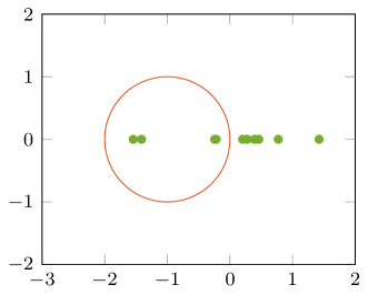
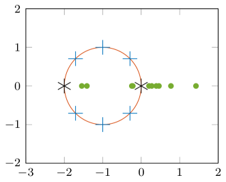
Figure 1: The eigenvalues are marked as (⚫) and a contour, in red, encircles the negative eigenvalues. On the right, a discretization of the contour is shown with $K=8$ equidistant points on the circle $z_{k}=-1+\cos(2k\pi/8)+i\sin(2k\pi/8)$. This leads to 6 complex poles (${\color[rgb]{0,0.4470,0.7410}+}$) and 2 real poles ($\ast$), i.e., 6 resolvents to be computed for $z_{k}\notin\mathbb{R}$ and 2 resolvents for $z_{k}\in\mathbb{R}$.

2.2 Quantum-native representation of rational transformations

On a quantum computer, we aim to evaluate the resolvent using ideally simple unitary circuits, although the resolvent is typically non-unitary. In this work, we consider Hamiltonian simulations $e^{-iHt}$ as the central algorithmic ingredient due to its feasibility on both digital and analog quantum platforms. Specifically, we can represent the resolvent in terms of unitary time evolution circuits through the following integral transformation

$$R(z_{k})=(z_{k}-H)^{-1}=\int_{0}^{\infty}dq\int_{-\infty}^{\infty}dy\,\kappa_{k}(q,y)e^{iy(z_{k}-H)q},$$ (3)

defined by some suitable choice of the integral kernel $\kappa_{k}\mathrel{\mathop{\mathchar 58\relax}}\mathbb{R}\times\mathbb{R}\rightarrow\mathbb{C}$ [13, 25, 57]. We immediately observe that the term $e^{iy(z_{k}-H)q}$ can be implemented by a time evolution of duration $t=yq$ under the Hamiltonian $H$. Since practical simulations favor shorter time evolutions, we seek a kernel for which $\kappa_{k}(q,y)e^{iyz_{k}q}$ decays sufficiently rapidly. In addition to satisfying Eq. 3, this requirement can impose further restrictions on the functional form of the kernel.

The distinction between poles off the real line (complex poles) and on the real line (real poles) turns out to be essential, because we will adopt different integral representations for these two separate cases. For a complex pole, the imaginary part leads to an exponentially decaying integrand. This means that a Dirac-delta kernel $\kappa_{k}(q,y)=-i\delta(y-1)$ can be employed for the case $\Im z_{k}>0$, which reduces the double integral in Eq. 3 to a single integral,

$$R(z_{k})=-i\int_{0}^{\infty}dq\,e^{-b_{k}q}\,e^{i(a_{k}-H)q},\qquad z_{k}=a_{k}+ib_{k},$$ (4)

equivalent to the Laplace transform of the matrix inverse (see also [57, Chapter 9]). The restriction to $\Im z_{k}>0$ is without loss of generality, since for a pole $z_{k}$ with $\Im z_{k}<0$ we can use the identity $R^{\dagger}(z_{k})=R(z_{k}^{\ast})$, where $\dagger$ and $\ast$ denote the Hermitian and complex conjugation, respectively.

The integral can be discretized by a quadrature rule [21, 15], which approximates the integral as a weighted sum specified by a set of nodes $\{t_{j}\}_{j=0}^{J-1}$ and corresponding weights $\{w_{j}\}_{j=0}^{J-1}$,

$$\int_{t_{\rm min}}^{t_{\rm max}}f(t)w(t)dt\approx\sum_{j=0}^{J-1}w_{j}f(t_{j})=\mathrel{\mathop{\mathchar 58\relax}}\mathcal{I}_{J},\qquad t_{j}\in[t_{\rm min},t_{\rm max}].$$ (5)

A common choice are the so-called Gaussian quadrature rules, which integrate polynomials up to degree $2J-1$ exactly using only $J$ nodes (the highest possible degree for any quadrature with $J$ nodes) [21]. The nodes and weights of a Gaussian quadrature rule depend on the weight function $w(t)$ and the integration interval $[t_{\rm min},t_{\rm max}]$.

Keen, Dumitrescu, and Wang [25] considered a simple quadrature rule, the trapezoidal rule, to discretize the integral of Eq. 4,

$$R(z_{k})\approx-i\sum_{j=0}^{J-1}w_{j}e^{(ia_{k}-b_{k})t_{j}}e^{-iHt_{j}}=\mathrel{\mathop{\mathchar 58\relax}}-i\sum_{j=0}^{J-1}x_{j}e^{-iHt_{j}},$$ (6)

with equidistant time samples $t_{j}=j\Delta t$ spaced apart by time step $\Delta t$ and weights $w_{j}=1/J$. We choose to absorb the scalar function $e^{(ia_{k}-b_{k})t_{j}}$ into the weights, leading to $x_{j}=e^{(ia_{k}-b_{k})t_{j}}w_{j}=\frac{e^{(ia_{k}-b_{k})t_{j}}}{J}$, to stress that the Hamiltonian simulations $e^{-iHt_{j}}$ are performed on a quantum computer, and the weighted sum of measurements of these real-time evolutions could be done classically. As the integrand is a non-periodic function, the trapezoidal rule converges only quadratically [15], i.e., the error decays slowly at the rate of $\mathcal{O}(\Delta t^{2})$. Therefore, a small $\Delta t$ is needed to obtain an accurate approximation, requiring a large number of samples $J$.

For a real pole, the integrand in Eq. 3 picks up a purely oscillatory phase without any decay. In this case, a rapid exponential decay can be introduced from an appropriate Gaussian kernel [13]. In particular, when the pole falls outside the spectral range, i.e., $z_{k}=a_{k}\in\mathbb{R}\setminus[E_{0},E_{N-1}]$ with $E_{0}$ and $E_{N-1}$ being the smallest and largest eigenvalues of $H$, the Gaussian kernel

$$\kappa_{k}(y)=\frac{1}{\pi}{\rm sgn}(a_{k}-E_{0})e^{-y^{2}/2},$$ (7)

leads to the double integral formulation,

$$R(z_{k})=\frac{1}{\pi}{\rm sgn}(a_{k}-E_{0})\int_{0}^{\infty}dq\,\int_{-\infty}^{\infty}dy\,e^{-y^{2}/2}e^{iy(a_{k}-H)q}.$$ (8)

We remark that when the pole does fall in the spectral range, i.e., $a_{k}\in[E_{0},E_{N-1}]$ and $a_{k}\neq E_{n}$ for $n=0,1,\dots,N-1$, a modified Gaussian kernel $\frac{i}{2\pi}qe^{-y^{2}/2}$ with an additional linear factor $q$ realizes a suitable resolvent representation. We will not discuss this case further, but the results presented in the paper can be readily generalized. The double integral in Eq. 8 can be discretized in two steps. We first discretize the inner $y$-integral,

$$R(z_{k})\approx\frac{1}{\pi}{\rm sgn}(a_{k}-E_{0})\sum_{\ell=0}^{L-1}x_{y,\ell}\int_{0}^{\infty}dq\,e^{-y_{\ell}^{2}/2}e^{iy_{\ell}(a_{k}-H)q}.$$ (9)

Now by recognizing Eq. 9 as a sum of integrals, each of the form as in Eq. 4, we then discretize the remaining integrals over $q$ as before. Childs, Kothari, and Somma [13] suggested discretizing both integrals via the trapezoidal rule. The discretization of the $y$-integral using a trapezoidal rule converges exponentially [52]. However, we would seek improved convergence for the $q$-integral by considering a different quadrature rule.

Discrete-time approach.

We refer to discretizing the integral representation via a quadrature rule as the discrete-time approach, since it allows us to compute the resolvent by sampling real-time evolutions (Hamiltonian simulations) at some discrete set of time points. This means that we can implement a rational function $r$ evaluated in an operator as a linear combination of unitaries, more precisely, of real-time evolutions,

$$r(H)\approx\sum_{j=0}^{J-1}x_{j,d}e^{-iHt_{j}},\qquad x_{j,d}=x_{j,d}(\bm{\kappa},\bm{c},\bm{z})~{}{\rm and}~{}t_{j}=t_{j}(\bm{c},\bm{z}),$$ (10)

where $t_{j}$ gives the simulation time and $x_{j,d}$ the associated ‘weight’ (with the subscript $d$ indicating discrete-time). The bold symbols in Eq. 10 represent vector-valued quantities of their respective dimensions. For example, $\bm{c}=(c_{0},\cdots,c_{K-1})$ and $\bm{z}=(z_{0},\cdots,z_{K-1})$ denote the sets of weights and poles in Eq. 1. Similarly, we denote our time grid as $\bm{t}=(t_{0},\cdots,t_{J-1})$ with $t_{j}\leq t_{j+1}$.

Continuous-time approach.

In contrast to the discrete-time approach, we explore alternative Hamiltonian simulations that avoid an explicit time discretization. Instead, we expand the kernel $\kappa_{k}$ in the integral representation with a set of simple basis functions. This allows us to decompose an exact representation of the resolvent into integral components that are efficiently constructible. Specifically, we choose a Gaussian basis set to approximate the integrand, which, as we will show, can be physically realized with continuous-variable ancillary wavefunctions [11, 31]. Analogous to Eq. 10, a rational function can be implemented as a linear combination of real-time evolutions that couple the system and Gaussian ancillae,

$$r(H)\approx\sum_{j=1}^{G}x_{j,c}\left({\rm Id}\otimes\bra{0_{j}}_{c}\right)e^{-i\tilde{H}}\left({\rm Id}\otimes\ket{0_{j}}_{c}\right),\qquad x_{j,c}=x_{j,c}(\bm{\kappa},\bm{c},\bm{z}),$$ (11)

where $\ket{0_{j}(\bm{c},\bm{z})}_{c}$ denotes a Gaussian ancillary state of some characteristic width, $G$ is the number of such Gaussian states, and $\tilde{H}$ describes an effective Hamiltonian that acts jointly on the system and ancillae. Here ${\rm Id}$ is the identity operator on the system Hilbert space. Notably, the effective Hamiltonian is evolved for a unit duration, which can be simulated directly without time sampling. To make a distinction, we refer to this Gaussian-based approach as the continuous-time approach.

In both discrete- and continuous-time approaches, we remark that the Hamiltonian simulations can be either performed individually, or combined coherently in a single quantum circuit through block-encoding (BE) [14, 8], a common routine to represent non-unitary operators on a quantum computer. In addition to time evolution, a block-encoding circuit calls two important subroutines, the prepare (PREP) and select (SEL) oracles. For example in the discrete-time approach, the PREP oracle encodes the coefficients $x_{j}$ into a superposition state $\sum_{j}x_{j}\ket{j}$ on auxiliary qubits, and the SEL oracle selectively applies Hamiltonian simulations $e^{-iHt_{j}}$ conditioned on the auxiliary index $j$. We write $(\alpha,m,\epsilon)$-BE for a block encoding $U_{\rm BE}$ which uses a renormalization factor $\alpha$, requires $m$ ancilla qubits, and incurs additive error $\epsilon$, i.e., $\lVert r(H)-\alpha\bra{0^{m}}U_{\rm BE}\ket{0^{m}}\|_{2}\leq\epsilon$.

Overall, we will refer to $r(H)$ as a quantum rational transformation (QRT) when a rational function $r(\omega)$ is applied to a Hermitian operator $H$ on quantum hardware using techniques such as those exemplified above.

3 Improved discrete-time LCU construction of a resolvent

The choice of quadrature rules for approximating the integral transformation Eq. 3 is essential for the development of efficient quantum algorithms based on resolvents. On one hand, the quadrature rule determines the rate of convergence of the approximation in Eq. 5 while, on the other hand, it prescribes the time evolutions that must be performed. Fig. 2 outlines the discrete-time LCU approach for sampling a resolvent $R(z)=(z-H)^{-1}$ with $z\notin\mathbb{R}$.

Figure 2: Discrete-time construction of a resolvent $R(z)=(z-H)^{-1}$, with a complex pole $z=a+bi$, via a quadrature rule given by the nodes $\{t_{j}\}_{j}$ and weights $\{w_{j}\}_{j}$, i.e., $R(z)\approx\sum_{j}w_{j}e^{(ia-b)t_{j}}e^{-iHt_{j}}$. On quantum hardware the Hamiltonian simulations $U(t_{j})=e^{-iHt_{j}}$ can be performed efficiently. The circuit diagram depicts Trotterized time evolution with multiple fixed steps $\Delta t$ and a final variable step $\delta t_{j}$, so that $U_{\rm Trotter}(\delta t_{j})U_{\rm Trotter}(\Delta t)^{M_{j}}\approx U(t_{j})$ for $t_{j}=M_{j}\Delta t+\delta t_{j}$. Repeated measurements in the computational basis enable us to access scalar quantities such as $\langle\phi|U_{\rm Trotter}(\delta t_{j})U_{\rm Trotter}(\Delta t)^{M_{j}}|\phi\rangle$, which can be collected and combined in post-processing to obtain the desired inner product $\langle\phi|R(z)|\phi\rangle$.

The current discretization standard is the trapezoidal rule [13, 25, 47, 56], which uses equidistant time sampling for Hamiltonian simulation but converges slowly for resolvent approximation. To address this, we analyze quadrature rules with non-equidistant nodes, which can significantly improve convergence. In Table 1, we list different quadrature rules considered in this work along with their key properties. The second column shows node distribution, with only the trapezoidal rule featuring equidistant nodes. The third and fourth columns quantify two time metrics dependent on the node distribution. These metrics follow from classical results on orthogonal polynomials [49] and are paramount to our cost analysis. For the trapezoidal rule, the weights are uniformly set at $w_{j}\equiv 1/J$. For the Gauss–Legendre, –Laguerre, and –Hermite rules, the nodes are the roots of orthogonal polynomials and the weights are chosen to optimally approximate the integrals from the last column [21]. Note that for the trapezoidal and Legendre rule the associated weight function is $w(t)\equiv 1$, whereas for the Laguerre and Hermite rule these are rapidly decaying, $w(t)=e^{-t}$ and $w(t)=e^{-t^{2}}$ respectively. These weight functions influence the associated quadrature weights.

Quadrature rule	Node distribution $\{t_{j}\}_{j=0}^{J-1}$	Maximal time $\max_{j}|t_{j}|$	Total time $\sum_{j}|t_{j}|$	Integral
Trapezoidal		Controllable $-\log(\epsilon b)/b$	$\frac{TJ}{2}$	$\int_{-1}^{1}f(t)dt$ $f(x)$ periodic!
Legendre		Controllable $-\log(\epsilon b)/b$	$\frac{TJ}{2}$	$\int_{-1}^{1}f(t)dt$
Laguerre		Uncontroll. $\approx 4J+2$	$J^{2}$	$\int_{0}^{\infty}f(t)e^{-t}dt$
Hermite		Uncontroll. $\approx\sqrt{2J}$	$\frac{3}{5}J^{3/2}$(⋆)	$\int_{-\infty}^{\infty}f(t)e^{-t^{2}}dt$

Table 1: Properties of quadrature rules considered for the discrete-time LCU approach to approximate the resolvent $R(z)=(z-H)^{-1}$ with an operator-norm error of $\mathcal{O}(\epsilon)$, where $z=a+bi$. In the second column we show the distribution of $J=20$ nodes. The cost parameter $T=\max_{j}|t_{j}|$ determines the length of the interval for the trapezoidal or Legendre rule (see [49, 21, 52] for details), and therefore the maximal runtime of the $J$ Hamiltonian simulations. The last column displays the integral for which the quadrature rule is optimal in the Gaussian sense. Note that any finite interval $[0,T]$ can be mapped linearly onto $[-1,1]$. For the trapezoidal/Legendre rule, the maximal runtime can be controlled a priori provided that $\epsilon$ and $b$ are known. For the Laguerre/Hermite rule, the maximal time depends on $J$ which is harder to quantify a priori. ^(⋆)The total runtime for the Hermite rule is determined empirically.

In this work, we consider using the Legendre rule for the $q$-integral and trapezoidal rule for the $y$-integral in Eq. 3. In Section 3.1, we argue that the Legendre rule is best suited for the $q$-integral, making it the preferred discrete-time LCU approach for resolvents with complex poles. We further quantify the cost of constructing an $\epsilon$-approximation to a resolvent in terms of the simulation time metrics. This is among the first (nonasymptotic) detailed cost analysis for quantum hardware. Section 3.2 supports our findings with numerical examples. Section 3.3 shifts focus to quadrature rules for resolvents with real poles, especially discretizing the $y$-integral. We propose combining the Legendre and the trapezoidal rules, instead of the common trapezoidal combination. A detailed cost analysis is presented, and numerical experiments in Section 3.4 show that this combination outperforms others. While our discussion is restricted to single poles, a generalization to repeated poles of higher multiplicities is provided in Appendix B.

3.1 Dirac-delta kernel for complex poles

For complex poles, i.e., $z_{k}=a_{k}+ib_{k}$ with $b_{k}>0$, we consider the single integral representation of Eq. 4. This integral involves the function $f(t)=-ie^{-b_{k}t}e^{i(a_{k}-H)t}$ over the interval $[0,\infty)$. Using a quadrature rule as in Eq. 5, we approximate the integral with a sum $\mathcal{I}_{J}(z_{k})$. The following scheme highlights how three important quadrature rules can be applied. All three rules follow the same procedure outlined in Fig. 2, querying a set of real-time evolutions under $H$. The key difference between the rules is in the choice of nodes, i.e., the evolution times, as listed in Table 1.

After a change of variable $b_{k}q\mapsto t$, Table 1 seemingly suggests the use of a Gauss–Laguerre rule for approximating the integral in Eq. 4. Under specific regularity assumptions, the Laguerre rule indeed has the potential to converge exponentially fast [35]. However, precise assertions or results about the general rate of convergence remain undetermined.

The trapezoidal and Legendre rule require a finite interval. A truncation with $\epsilon$-control over the error can be obtained thanks to the exponential decay of the integrand, i.e.,

$$R(z_{k})\approx-i\int_{0}^{T_{k}^{\rm max}}dq\,e^{-b_{k}q}\,e^{i(a_{k}-H)q},\quad\text{with }T^{\rm max}_{k}=\lVert\bm{t}\rVert_{\infty}=\frac{1}{b_{k}}\log\frac{1}{\epsilon b_{k}}.$$ (12)

While a trapezoidal discretization, $t^{\rm Trap}_{j}=j\Delta t$ for the fixed timestep $\Delta t=\frac{T_{k}^{\rm max}}{J-1}$, is commonly assumed for real-time algorithms [25], it can result in a large total simulation time $T^{\rm tot}_{k}=\lVert\bm{t}\rVert_{1}$. This is because the trapezoidal rule applied to the nonperiodic truncated integral in Eq. 12 suppresses the approximation error slowly as the number of timesteps increases, i.e., at an algebraic rate of $\mathcal{O}\left(\frac{1}{\Delta t^{2}}\right)$ [15].

In this paper, we propose the use of the Gauss–Legendre quadrature rule. Observe that upon changing the variable $q\mapsto\frac{T_{k}^{\rm max}(1+t)}{2}$,

$$R(z_{k})\approx-\frac{iT_{k}^{\rm max}}{2}\int_{-1}^{1}dt\,e^{-b_{k}T_{k}^{\rm max}(1+t)/2}e^{i(a_{k}-H)T_{k}^{\rm max}(1+t)/2}\approx\mathcal{I}^{\rm Leg}_{J}(z_{k}),$$ (13)

where for $\mathcal{I}^{\rm Leg}_{J}(z_{k})$ we take $\bm{t}\in[-1,1]^{J}$ to be the roots of the degree-$J$ Legendre polynomial. For exponentially decaying integrands, it is known that the Legendre rule achieves similar accuracy as the Laguerre rule [18]. Moreover the Legendre rule establishes a robust exponential convergence, which allows us to favorably reduce the number of distinct real-time circuits $J$. In particular, the convergence follows from the classical results [54, 21] that the Gauss–Legendre error for a function $f$ which is analytic within and on the ellipse, $\mathcal{E}_{\sigma}=\left\{\frac{\sigma}{2}e^{i\theta}+\frac{1}{2\sigma}e^{-i\theta}\mathrel{\mathop{\mathchar 58\relax}}\theta\in[-\pi,\pi]\right\}$, is bounded by

$$e_{J}[f;\mathcal{E}_{\sigma}]\leq\frac{8\sigma^{2}\sup_{t\in\mathcal{E}_{\sigma}}\lvert f(t)\rvert}{\sigma^{2J}(\sigma^{2}-1)},$$ (14)

where $e_{J}[f]$ labels the difference between the exact and discretized $f$-integral over $[-1,1]$. Since the integrand in Eq. 13, $f(t)=e^{i(z_{k}-H)T^{\rm max}_{k}(1+t)/2}$, is analytic on the whole complex plane, this error bound holds for every $\sigma>1$. With a fixed $\sigma$, the approximation accuracy hence improves exponentially with respect to $J$, highlighting the advantage of the Legendre rule over the algebraic convergence of the trapezoidal rule. Its efficiency, in terms of quantum resources, is summarized in the following theorem.

Theorem 1.

For a complex pole $z_{k}=a_{k}+ib_{k}$ with $b_{k}>0$ and any tolerance $\epsilon>0$, the resolvent $R(z_{k})$ admits a real-time LCU construction $\mathcal{I}_{J}(z_{k})$ for which $\lVert R(z_{k})-\mathcal{I}_{J}(z_{k})\rVert_{2}<\epsilon$. The Gauss–Legendre rule defines a time grid $\bm{t}$ such that

$$J=\log_{2}\log\frac{2}{\epsilon b_{k}}+(\eta_{k}+1)\log_{2}\frac{2}{\epsilon b_{k}}+3$$ (15)

distinct time evolution circuits suffice to construct $\mathcal{I}_{J}(z_{k})$, where $\eta_{k}=\frac{3b_{k}-2\sqrt{2}b_{k}+a_{k}^{+}}{4\sqrt{2}b_{k}}$ and $a_{k}^{+}=\max_{0\leq n\leq N-1}\lvert a_{k}-E_{n}\rvert$ for eigenvalues $E_{n}$ of $H$. The corresponding maximal and total evolution time is given by, respectively,

$$T^{\max}=\lVert\bm{t}\rVert_{\infty}=\frac{1}{b_{k}}\log\frac{2}{\epsilon b_{k}},\qquad\text{and}\qquad T^{{\rm tot}}=\lVert\bm{t}\lVert_{1}=\frac{J}{2b_{k}}\log\frac{2}{\epsilon b_{k}}.$$ (16)

Proof.

The proof is provided in Section A.1. ∎

The constant $\eta_{k}$ in 1 is critical for determining the quantum resources since it lacks a logarithmic dependence on the resolvent parameters. Importantly, $\eta_{k}$ can be systematically reduced if we place the pole $z_{k}$ farther from the real line. We remark that implementing the trapezoidal rule with the exact same maximal runtime necessitates $J=\left[\frac{1}{\epsilon b_{k}}\log\frac{2}{\epsilon b_{k}}\right]$ Hamiltonian simulations and a total runtime of $T^{\rm tot}=\frac{1}{2\epsilon b_{k}^{2}}\left[\log\frac{2}{\epsilon b_{k}}\right]^{2}$ [25]; our result achieves a respective enhancement by multiplicative factors of $\frac{1}{\epsilon}$ and $\frac{1}{\epsilon}\left[\log\frac{1}{\epsilon}\right]^{-1}$. Hence, the Gauss–Legendre rule offers a simple, improved LCU recipe that can lead to substantial resource reduction for resolvent computation.

Given access to the PREP and SEL oracles, 1 states that the discrete-time approach can be alternatively viewed as a $(1,\lceil\log_{2}J\rceil,\epsilon)$ BE of the resolvent.

3.2 Numerical experiments for complex poles

We now illustrate 1 for the 1D mixed-field Ising model (MFIM),

$$H=-\sum_{i=1}^{L_{\rm sys}}Z_{i}Z_{i+1}-h\sum_{i=1}^{L_{\rm sys}}Z_{i}-g\sum_{i=1}^{L_{\rm sys}}X_{i},$$ (17)

where $h$ and $g$ set the longitudinal and transverse field, respectively, and $L_{\rm sys}$ denotes the number of spins. For simplicity, we assume $\lVert H\rVert_{2}\leq 1$ by rescaling the spectrum $H\mapsto\frac{H}{\|H\|_{2}}$.

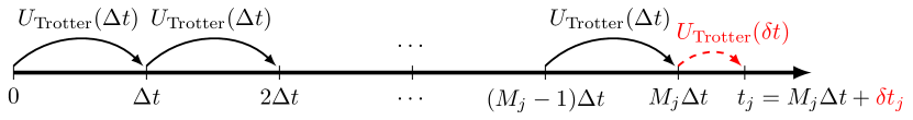
Figure 3: Simulation of $e^{-iHt_{j}}$ by Trotterized time evolution $U_{\rm Trotter}(t)\mathrel{\mathop{\mathchar 58\relax}}=e^{-iH_{1}t}e^{-iH_{2}t}$. The evolution is advanced for multiple fixed time steps $\Delta t$, common for all simulations $t_{j}\in\bm{t}$, and a variable shorter time step $\delta t_{j}<\Delta t$ dependent on $t_{j}$.

To implement the real-time evolution $e^{-iHt}$, we employ a Trotter splitting $H=H_{1}+H_{2}$, where $H_{1}=-\sum_{i}Z_{i}Z_{i+1}-h\sum_{i}Z_{i}$ and $H_{2}=-g\sum_{i}X_{i}$ can be simulated efficiently. For $M$ Trotter steps, each of size $\Delta t=\frac{t}{M}$, the first-order Trotter scheme reads $e^{-iHt}\approx\left(e^{-iH_{1}\Delta t}e^{-iH_{2}\Delta t}\right)^{M}$ and incurs an error of $\mathcal{O}(t\Delta t)$ [32]. This implies a Trotter step size of $\Delta t=\frac{\epsilon}{T^{\rm max}}$ to reach a target accuracy of $\epsilon$ for all $t_{j}\in\bm{t}$. For equidistant nodes $\bm{t}$ of the trapezoidal rule, a fixed Trotter step size suffices to simulate the $J$ evolutions $e^{-iHt_{j}}$ necessary to construct a resolvent. However, the distance between adjacent Laguerre or Legendre nodes is not constant. In this case, we take

$$e^{-iHt_{j}}\approx\left(e^{-iH_{1}\Delta t}e^{-iH_{2}\Delta t}\right)^{M_{j}}e^{-iH_{1}\delta t_{j}}e^{-iH_{2}\delta t_{j}},$$ (18)

where each $t_{j}\in\bm{t}$ is approached as closely as possible by $M_{j}$ $\Delta t$-steps and a final variable step of size $\delta t_{j}<\Delta t$, as is illustrated in Fig. 3.

Convergence as a function of simulation time.

For the MFIM with $L_{\rm sys}=8$ spins, we verify that the Legendre rule outperforms the trapezoidal and Laguerre rules. We fix the Hamiltonian model parameters $(h,g)=(1,\frac{2}{3})$, and consider the complex pole $z=-0.8+0.1i$. Fig. 4 displays the approximation error $\|R(z)-\mathcal{I}_{J}(z)\|_{2}$ relative to the scaled total evolution time $\frac{T^{\rm tot}}{T^{\rm max}}$ for the different quadrature rules and requested accuracy of $\epsilon=10^{-3}$ and $\epsilon=10^{-6}$. We take a Trotter step of $\Delta t=\epsilon$. The trapezoidal rule shows an algebraic convergence, while the Laguerre rule converges exponentially and incurs a simulation cost $T^{\rm tot}=\mathcal{O}(J^{2})$. The Legendre rule converges exponentially and is the most efficient. We also note that the onset of the convergence of the Legendre rule occurs earlier for lower requested accuracy, since the truncation $T^{\rm max}$ is smaller in this case, making the truncated integral easier to approximate.

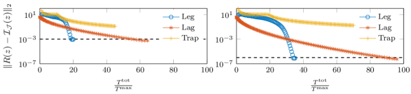
Figure 4: Approximation error $\|R(z)-\mathcal{I_{J}}(z)\|_{2}$ as a function of the scaled total evolution time $\frac{\|\bm{t}\|_{1}}{T^{\rm max}}$, for $z=-0.8+0.1i$ and the (scaled) MFIM Hamiltonian with $L_{\rm sys}=8$ spins. The approximation $\mathcal{I_{J}}(z)$ is computed using the trapezoidal (+), Legendre ($\circ$) and Laguerre ($\ast$) rule for a requested accuracy of $\epsilon$ ($10^{-3}$ left and $10^{-6}$ right) and Trotter step of $\Delta t=\epsilon$.

Simulation time as a function of pole position.

Eq. 16 indicates that a pole closer to the real line is more costly to simulate. For selected poles $z_{k}$, a target accuracy $\epsilon=10^{-6}$, and Trotter step $\Delta t=\frac{\epsilon}{T^{\rm max}}$, we report the cost $\frac{T_{k}^{\rm tot}}{T_{k}^{\rm max}}$ for each of the quadrature rules to obtain an $\epsilon$-approximation satisfying $\|R(z_{k})-\mathcal{I}_{J}(z_{k})\|_{2}<\epsilon$. We also report the predicted cost in terms of the total evolution time for the Legendre rule in Eq. 15 and Eq. 16. Fig. 5 shows these quantities for poles $z_{k}=-0.8+2^{-k+1}i$ (left pane) and $z_{k}=2^{-k+1}i$ (right pane), with $k=1,\dots,6$. The Legendre rule proves to be the most efficient for all considered poles $z_{k}$. The Laguerre rule leads to numerical underflow for $z_{k}=-0.8+2^{-4}i$ and $z_{k}=2^{-5}i$ before reaching the target accuracy, whereas the trapezoidal rule appears orders of magnitude more expensive. We only compare data where the cost is below or approximately $10^{4}$. The predicted cost for the Legendre rule captures the overall trend of the actual cost as the pole moves closer to the real line. The difference between the two panes is attributed to the largest distance $a^{+}$ of the poles from an eigenvalue measured on the real line (and therefore independent on $k$ in this experiment). A larger $a^{+}$ increases the cost for all considered quadrature rules.

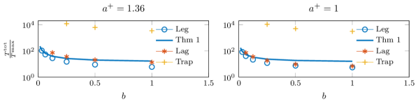
Figure 5: Cost $\frac{\|\bm{t}\|_{1}}{T^{\rm max}}$ for quadrature rules necessary to compute an $\epsilon$-approximation to $(z-H)^{-1}$ with accuracy $\epsilon=10^{-6}$. A Trotter step of $\Delta t=\frac{\epsilon}{T^{\rm max}}$ is used to evolve the MFIM Hamiltonian with $L_{\rm sys}=8$ spins. We consider $z=-0.8+bi$ on the left and $z=bi$ on the right, which yields $a^{+}=1.36$ and $a^{+}=1$ respectively. The Legendre rule ($\circ$) performs more efficiently than the Laguerre ($\ast$) and trapezoidal ($+$) rule. The solid line shows the predicted cost for the Legendre rule derived in 1.

We comment that similar results for Heisenberg spin systems of varying dimensions and lattice geometries are presented in Appendix C.

3.3 Gaussian kernel for real poles

For a real pole outside the spectral range, i.e., $z_{k}=a_{k}\in\mathbb{R}$ and $a_{k}\notin[E_{0},E_{N-1}]$, the resolvent can be represented as the double integral of Eq. 8. For clarity and ease of notation, we will omit the overall sign factor from here on.

Eq. 9 suggests that the resolvent can be approximated in two steps. First the inner $y$-integral can be discretized, and afterwards the $q$-integrals can be efficiently recovered by the Legendre rule as justified in Section 3.1. Thus, for the remainder of this section we only examine discretization of the inner $y$-integral. The following scheme provides an overview of the quadrature rules to be discussed.

Gauss–Hermite quadrature, with its nodes being the roots of the degree-$L$ Hermite polynomial, appears to be a natural candidate as suggested by Table 1. The Gauss–Hermite rule can be applied to the inner $y$-integral in Eq. 8 after a change of variable $\frac{y}{\sqrt{2}}\mapsto t$. Unfortunately, the lack of a tractable error analysis generally complicates the estimation of quantum resources, much like the case of the Laguerre quadrature rule for the $q$-integral.

In this work, we $\epsilon$-truncate the $y$-integral by exploiting the exponential decay of the integrand,

$$R(z_{k})\approx\frac{1}{\pi}\int_{0}^{\infty}dq\int_{-y^{\rm max}}^{y^{\rm max}}dye^{-y^{2}/2}e^{iy(a_{k}-H)q},\quad\text{with }\pm y^{\rm max}=\pm\sqrt{\log\frac{1}{\epsilon a_{k}^{-}}}.$$ (19)

This truncation allows for the use of the trapezoidal and Legendre rule. The Legendre rule achieves exponential convergence, which follows from similar arguments as those in Section 3.1. The trapezoidal rule, $y_{\ell}=(\ell-\frac{L-1}{2})\Delta y$ with $\Delta y=\frac{2y^{\rm max}}{L-1}$, also converges exponentially based on the fact that the integrand function is quasi-periodic on the interval $[-y^{\rm max},y^{\rm max}]$, i.e., $f(-y^{\rm max})=f(y^{\rm max})+\mathcal{O}(\delta)$ for a small $\delta$ that can be controlled by the truncation parameter $y^{\rm max}$. The trapezoidal rule converges exponentially up to an accuracy $\mathcal{O}(\delta)$: this is a well-established result for integration of rapidly decaying analytic functions [52]. In particular, the trapezoidal error for a function $f$ that is analytic in the horizontal strip, $\mathcal{S}_{\sigma}=\left\{\omega\mathrel{\mathop{\mathchar 58\relax}}\mathinner{\!\left\lvert\Im\omega\right\rvert}\leq\sigma\right\}$, is bounded by,

$$e_{\Delta y}[f]\leq\frac{2\sup_{s\in[-\sigma,\sigma]}\int_{-\infty}^{\infty}dy\,\lvert f(y+is)\rvert}{e^{2\pi\sigma/\Delta y}-1},$$ (20)

where $e_{\Delta y}[f]$ gives the approximation error of the exact $f$-integral over $(-\infty,\infty)$ with a discretization step $\Delta y$.

Building upon 1, we quantify the resource efficiency of the combined Legendre ($q$-integral) and trapezoidal ($y$-integral) rule for approximating Eq. 8 in the following theorem.

Theorem 2.

For a real pole $z_{k}=a_{k}\in\mathbb{R}$ with $a_{k}\notin[E_{0},E_{N-1}]$ and any tolerance $\epsilon>0$, the resolvent $R(z_{k})$ admits a real-time LCU construction $\mathcal{I}_{J}(z_{k})$ for which $\lVert R(z_{k})-\mathcal{I}_{J}(z_{k})\rVert_{2}<\epsilon$. Let the truncation parameter $y^{\rm max}$ be chosen such that the $y$-integrand is periodic up to a $\delta$-perturbation with $\mathcal{O}(\delta)<\epsilon$. Then the combination of the Gauss–Legendre (q-integral) and trapezoidal (y-integral) rules defines a time grid $\bm{t}$ such that, up to leading order,

$$\begin{split}J=\bigg{[}\log\frac{32e^{\pi}}{\sqrt{\pi}\epsilon^{2}a_{k}^{+}a_{k}^{-}}+\frac{2\sqrt{2}a_{k}^{+}}{a_{k}^{-}}\log\frac{4}{\epsilon a_{k}^{-}}\bigg{]}\bigg{[}\log_{2}\frac{\sqrt{2}}{\pi\epsilon a^{-}_{k}}+\frac{a_{k}^{+}}{2a_{k}^{-}}\log_{2}\frac{4}{\epsilon a_{k}^{-}}+7\bigg{]}\end{split}$$ (21)

distinct time evolution circuits suffice to construct $\mathcal{I}_{J}(z_{k})$, where $a_{k}^{+}=\max_{0\leq n\leq N-1}\lvert a_{k}-E_{n}\rvert$ and $a_{k}^{-}=\min_{0\leq n\leq N-1}\lvert a_{k}-E_{n}\rvert$ for eigenvalues $E_{n}$ of $H$. Additionally, the maximal and total evolution time can also be controlled by

$$T^{\max}=\lVert\bm{t}\rVert_{\infty}=\frac{2\sqrt{2}}{a_{k}^{-}}\log\frac{4}{\epsilon a_{k}^{-}},\qquad\text{and}\qquad T^{\rm tot}=\lVert\bm{t}\lVert_{1}=\frac{\sqrt{2}J}{2a_{k}^{-}}\log\frac{4}{\epsilon a_{k}^{-}}.$$ (22)

Proof.

The proof is provided in Section A.2. ∎

In 2, the condition number of the shifted operator, $\frac{a_{k}^{+}}{a_{k}^{-}}={\rm cond}(z_{k}-H)$, is essential in bounding the quantum resources cost. We notice that the asymptotic cost of employing the Dirac-delta kernel and the Gaussian kernel in the discrete-time LCU approach is comparable since $J=\mathcal{O}\big{(}\log{\rm poly}\frac{{\rm constant}}{\epsilon}\big{)}$ and $T^{\rm max}=\mathcal{O}\big{(}\log\frac{{\rm constant}}{\epsilon}\big{)}$ for both cases. Despite the same asymptotic dependence, the actual implementation cost can vary significantly between the kernels. Finally, we remark that the result for real poles is directly applicable to solving linear systems of equations, a routine fundamental in quantum linear algebra.

3.4 Numerical experiments for real poles

For the MFIM Hamiltonian in Eq. 17, we explore different discrete LCU constructions for poles on the real line. Again we consider the rescaled Hamiltonian with $(h,g)=(1,\frac{2}{3})$ and $L_{\rm sys}=8$.

Convergence as a function of simulation time.

We compare the three quadrature rules for the $y$-integral (Hermite, Trapezoidal, and Legendre) combined with a Legendre discretization of the $q$-integral. The first term in Eq. 21 provides an estimate for the number of Legendre nodes, $L_{q}\approx\log{\frac{32e^{\pi}}{\sqrt{\pi}\epsilon^{2}a_{k}^{+}a_{k}^{-}}}+\frac{2\sqrt{2}a_{k}^{+}}{a_{k}^{-}}\log{\frac{4}{\epsilon a_{k}^{-}}}$, required to reach a desired accuracy. However, as we have noticed that it often overestimates the optimal choice, we empirically determine $L_{q}$ closer to the optimal and report these values in Figs. 6 and 7. The convergence of the Legendre, trapezoidal, and Hermite rule is shown in the top panel of Fig. 6 for the real pole $z=-1.1$ and accuracy $\epsilon=10^{-6}$. While all three combinations exhibit an exponential rate of convergence, the onset of convergence occurs earliest for the trapezoidal rule, resulting in the most efficient approximation.

In the bottom panel of Fig. 6, we compare the current standard in literature [13], i.e., the trapezoidal rule for both integrals, to the proposed Legendre-trapezoidal combination which we find more efficient.

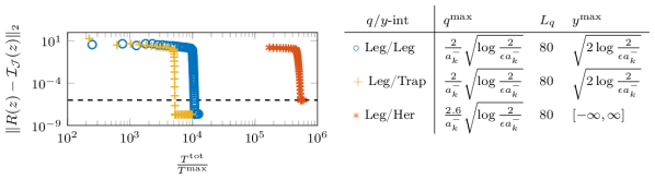
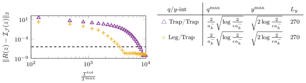
Figure 6: Error of quadrature approximations to $R(z_{k})$ for the MFIM Hamiltonian with $L_{\rm sys}=8$ spins, a requested accuracy $\epsilon=10^{-6}$, and $z_{k}=-1.1$, in terms of the cost $\frac{T^{\rm tot}}{T^{\rm max}}$. The table shows the parameter settings and quadrature rules used for the outer $q$-integral and inner $y$-integral. Top: Number of nodes $L_{y}$ to discretize the $y$-integral is varied. Bottom: Number of nodes $L_{q}$ to discretize the $q$-integral is varied. Note: $a_{k}^{-}=0.1$.

Simulation time as a function of pole position.

Eq. 21 implies that the cost of approximating $R(z_{k})$ increases as $z_{k}$ moves closer to an eigenvalue. In Fig. 7 we report the cost $\frac{T^{\rm tot}}{T^{\rm max}_{k}}$ required to approximate $R(z_{k})$ up to accuracy $\epsilon=10^{-6}$ as $z_{k}$ approaches $E_{0}$. The Hermite rule is significantly more expensive, and the trapezoidal rule is the most efficient. The estimate for $L_{q}$ suggests that for $z_{k}=-1-2^{-k-1}$ ($a_{k}^{-}=2^{-k-1}$) the number of nodes should increase approximately as $2^{k}$, yet the figure shows that a linearly increasing number of nodes is sufficient. The bound provided in Eq. 22, based on the $L_{q}$ reported next to the figure, is shown as the solid line in Fig. 7. It largely overestimates the observed cost and seems to exhibit different asymptotic behavior. The difference between the observed and predicted asymptotic behavior might be explained by the use of loose (pessimistic) bounds in the proof of Theorem 2. A more careful analysis of the errors could result in tighter bounds and a more accurate prediction of the asymptotic behavior, an important direction for future work.

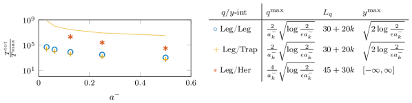
Figure 7: Cost $\frac{\|\bm{t}\|_{1}}{T^{\rm max}}$ for quadrature rules necessary to compute an $\epsilon$-approximation to $(z-H)^{-1}$ with accuracy $\epsilon=10^{-6}$. We consider $z=-1-2^{-k-1}$ for $k=0,1,\dots,4$. The solid line shows the cost predicted by 2 for the combination of Leg/Trap rule.

4 Continuous-time LCU construction of a resolvent

In general, the resources required for even an optimal Hamiltonian simulation must scale at least linearly with the simulation time, due to the no fast-forwarding theorem [7, 12]. This can make simulations over long time exceedingly costly, thus limiting the applicability of the discrete-time LCU approach elaborated within Section 3. In pursuit of a complementary strategy, we consider constructing the resolvent through the continuous-time LCU approach. This allows us to control the cost of Hamiltonian simulations by the introduction of continuous-variable ancilla [11].

The main idea behind the continuous-time approach is to associate the integral form of Eq. 3 with some spatially extended ancillary state, e.g., a continuous-variable wavefunction describing a harmonic oscillator. The ancilla is coupled to the system via a total Hamiltonian $\tilde{H}=H_{\rm sys}\otimes V$, where the system Hamiltonian $H_{\rm sys}(H;z_{k})$ contains the operator of interest $H$, and the ancillary potential $V(\hat{q},\hat{y};z_{k})$ is dependent on two (commuting) position operators $\hat{q}$ and $\hat{y}$. This approach requires hybrid quantum information processing which utilizes both discrete qubits and continuous Gaussian states [2, 31]. Fig. 8 illustrates the continuous-time LCU procedure for a complex pole $z\notin\mathbb{R}$, which involves sampling a set of 1D Gaussian ancillary wavefunctions.

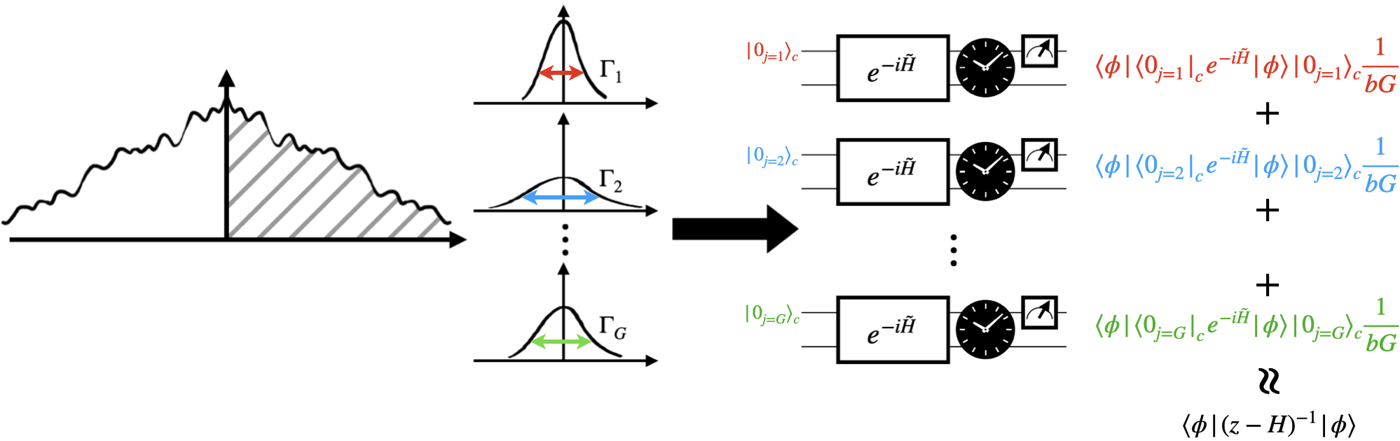
Figure 8: Continuous-time LCU construction of the resolvent $R(z)=(z-H)^{-1}$ via the Gaussian representation. The integral of a decaying oscillatory function is approximated using a weighted combination of Gaussian integrals of the form $\frac{1}{\sqrt{2\pi\Gamma}}\int_{-\infty}^{\infty}dq\,e^{-q^{2}/2\Gamma-i(a-H)\mathinner{\!\left\lvert q\right\rvert}}$. On quantum hardware the Hamiltonian simulation $U=e^{-i\tilde{H}}$ with a constant duration can be performed efficiently. The circuit diagram shows the composite evolution with ancilla prepared in the Gaussian state. Repeated measurements in the computational basis enable us to access scalar quantities such as $\langle\phi|\bra{0_{j}}_{c}e^{-i\tilde{H}}|\phi\rangle\ket{0_{j}}_{c}$, which can be collected and combined in post-processing to obtain $\langle\phi|R(z)|\phi\rangle$.

Within the framework of continuous-time LCU, efficient strategies to approximate the integral transform of Eq. 3 defined by the Dirac-delta and Gaussian kernels are proposed in Section 4.1 (complex poles) and Section 4.3 (real poles), respectively. Section 4.2 and Section 4.4 contain the corresponding numerical illustration on the MFIM Hamiltonian as considered in Section 3.

4.1 Dirac-delta kernel for complex poles

Formally, the continuous-time implementation requires the preparation of a single ancilla,

$$\ket{0}_{c}=\int_{0}^{\infty}dq\,\psi(q;b_{k})\ket{q}\mathrel{\mathop{\mathchar 58\relax}}=\sqrt{b_{k}}\int_{0}^{\infty}dq\,e^{-b_{k}q/2}\ket{q},$$ (23)

where we can reinterpret the integration variable $q$ as the ancillary position degree of freedom and $\psi(q)$ as the corresponding ancillary wavefunction. Observe that for the particular choice of $\psi(q)$ in Eq. 23, the imaginary part of the pole, $b_{k}$, determines the exponential decay in the wavefunction. A more general single-ancilla setup for encoding the resolvent is described later in this section and summarized in the following scheme.

We evolve the ancilla together with the system qubits under the total Hamiltonian $\tilde{H}\mathrel{\mathop{\mathchar 58\relax}}=(H-a_{k})\otimes\hat{q}$ for which $\hat{q}\ket{q}=q\ket{q}$. Since a time evolution of unit duration generates the composite state,

$$e^{-i\tilde{H}}\ket{\phi}\ket{0}_{c} =\int_{0}^{\infty}dq\,\psi(q)e^{i(a_{k}-H)q}\ket{\phi}\ket{q},$$ (24)

$$=\int_{0}^{\infty}dq\,\psi(q)e^{i(a_{k}-H)q}\ket{\phi}\psi^{\ast}(q)\ket{0}_{c}+\ket{\perp}=ib_{k}R(z_{k})\ket{\phi}\ket{0}_{c}+\ket{\perp},$$ (25)

where in the last equality we recover the integral transform of Eq. 4 using the ancilla wavefunction from Eq. 23, and the residual state $\ket{\perp}$ belongs to the kernel of the projector ${\rm Id}\otimes\ket{0}_{c}\bra{0}_{c}$. Therefore by post-selecting the ancilla, we can implement the action of a resolvent on any initial state $\ket{\phi}$, i.e., we can prepare the normalized state $iR(z_{k})\ket{\phi}/\lVert R(z_{k})\ket{\phi}\rVert_{2}$. The success probability of post-selection is given by

$$P_{R(z_{k})} =b_{k}^{2}\lVert R(z_{k})\ket{\phi}\rVert_{2}^{2}=\sum\limits_{n=0}^{N-1}\frac{p_{n}b_{k}^{2}}{\mathinner{\!\left\lvert a_{k}-E_{n}\right\rvert}^{2}+b_{k}^{2}},$$ (26)

where $p_{n}=\lvert\braket{E_{n}}{\phi}\rvert^{2}$ denotes the squared overlap between the $n$th eigenstate $\ket{E_{n}}$ of $H$ and the initial system state $\ket{\phi}$. The success probability depends on the initial state $\ket{\phi}$, the Hamiltonian spectrum ${\rm spec}(H)\mathrel{\mathop{\mathchar 58\relax}}=(E_{0},E_{1},\cdots,E_{N-1})$, and the pole position $z_{k}=a_{k}+ib_{k}$.

By Eqs. 24 and 25, we see that the continuous-time formulation imposes a minimal resource requirement for Hamiltonian simulation since $\lVert\bm{t}\rVert_{\infty}=\lVert\bm{t}\rVert_{1}=1$. Instead, the complexity of this equivalent formulation primarily lies in the preparation and measurement of the ancilla $\ket{0}_{c}$. Similar to the discrete setting, we may truncate the spatial integral at $T_{k}^{\rm max}$. However, despite the elementary analytical form of $\psi$, its accurate preparation on quantum hardware can be a nontrivial task, for example due to the discontinuity in the wavefunction at $q=0$. Ideally, we aim to exploit simple, smooth wavefunctions with rapid spatial decay.

To significantly simplify the ancilla initialization, we now express Eqs. 23 and 24 in an alternative representation in terms of Gaussians. By first symmetrizing the integral and then using a well-established identity that a Laplace distribution, $e^{-b_{k}\lvert q\rvert}$ in Eq. 27, can be represented exactly as a mixture of Gaussians with an exponential mixing density $\rho_{\rm mix}$ [42],

$$\int_{0}^{\infty}dq\,e^{-b_{k}q+i(a_{k}-H)q} =\frac{1}{2}\int_{-\infty}^{\infty}dq\,e^{-b_{k}\lvert q\rvert+i(a_{k}-H)\lvert q\rvert},$$ (27)

$$=\frac{1}{b_{k}}\int_{-\infty}^{\infty}dq\,\int_{0}^{\infty}d\Gamma\,\rho_{\rm mix}(\Gamma|b_{k})\varphi_{g}(q;\Gamma)e^{i(a_{k}-H)\lvert q\rvert},$$ (28)

with a centered Gaussian wavefunction of spatial variance $\Gamma$,

$$\varphi_{g}(q;\Gamma)=\frac{1}{\sqrt{2\pi\Gamma}}e^{-q^{2}/2\Gamma},$$ (29)

and, where $\rho_{\rm mix}(\Gamma)$ specifies a probability measure on all possible Gaussian variances,

$$\rho_{\rm mix}(\Gamma|b_{k})=\frac{b_{k}^{2}}{2}e^{-b_{k}^{2}\Gamma/2}.$$ (30)

Since $\rho_{\rm mix}$ is a probability measure, Eq. 28 can be understood as an expectation,

$$iR(z_{k}) =\frac{1}{b_{k}}\mathbb{E}_{\rm mix}\bigg{[}\int_{-\infty}^{\infty}dq\,\varphi_{g}(q;\Gamma)e^{i(a_{k}-H)\lvert q\rvert}\bigg{]}=\frac{1}{b_{k}G}\sum_{j=1}^{G}\underbrace{\int_{-\infty}^{\infty}dq\,\varphi_{g}(q;\Gamma_{j})e^{i(a_{k}-H)\lvert q\rvert}}_{\mathrel{\mathop{\mathchar 58\relax}}=A_{j}},$$ (31)

where $\mathbb{E}_{\rm mix}$ denotes an average with respect to $\rho_{\rm mix}$ computed from Monte-Carlo sampling. The stochastic representation enables us to deal exclusively with Gaussian states. This is advantageous since these correspond to the ground state of a quantum harmonic oscillator and constitute one of the most essential resources accessible in continuous-variable computing.

For each Monte-Carlo sample $\Gamma_{j}\sim\rho_{\rm mix}$, we now initialize the ancilla in the Gaussian state,

$$\ket{0_{j}}_{c}=\int_{-\infty}^{\infty}dq\,\sqrt{\varphi_{g}(q;\Gamma_{j})}\ket{q}.$$ (32)

Observe that for $\tilde{H}=(H-a_{k})\otimes\lvert\hat{q}\rvert$,

$$e^{-i\tilde{H}}\ket{\phi}\ket{0_{j}}_{c}=A_{j}\ket{\phi}\ket{0_{j}}_{c}+\ket{\perp_{j}},$$ (33)

where $\ket{\perp_{j}}$ encodes the orthogonal residual just as in the naïve case. Consequently, post-selection on the ancilla achieves stochastic filtering with success probability,

$$P_{A_{j}}=\left\lVert A_{j}\ket{\phi}\right\rVert_{2}^{2}=\sum_{n=0}^{N-1}p_{n}e^{-\Gamma_{j}E_{n}^{2}}\bigg{[}1+{\rm erfi}^{2}\bigg{(}\sqrt{\frac{\Gamma_{j}}{2}}E_{n}\bigg{)}\bigg{]},$$ (34)

where ${\rm erfi}(\cdot)$ is the imaginary error function.

Put differently, we have shown that the real-time evolution $e^{-i\tilde{H}}$ of unit duration can be viewed algorithmically as an efficient $(1,\mathbf{1},0)$-BE of the stochastic resolvent $A_{j}$, except that $(i)$ the ancilla is bosonic (we will use bold number to highlight this difference) and $(ii)$ its initialization depends on $A_{j}$. This approach avoids the need of discretizing the integral of Eq. 4 in time. Moreover, the maximal runtime of the Hamiltonian simulations, a major expense in the discrete-time LCU, becomes independent of the Hamiltonian structure or pole location. In exchange, the cost of ancilla initialization now reflects the dependence on the pole as suggested by Eq. 30. Here, preparing a broader Gaussian wavefunction, which results from a pole located closer to the real line, incurs a higher expense. This is due to the greater complexity in coherently loading and manipulating the wavefunction across a larger spatial region.

With such continuous-variable BE, we may formally implement the SEL and PREP oracles,

$$U^{\rm SEL}=-i\sum_{j=1}^{G}\ket{j}\bra{j}\otimes\big{(}e^{-i\tilde{H}}U_{c,j}\big{)},\qquad U^{\rm PREP}\ket{0^{\log_{2}G}}=\frac{1}{\sqrt{G}}\sum_{j=1}^{G}\ket{j},$$ (35)

where $U_{c,j}$ is a circuit capable of preparing the Gaussian ancilla $\ket{0_{j}}_{\rm c}$. For example, we can define $U_{c,j}\ket{e}_{c}=\ket{0_{j}}_{c}$ for a fixed ancillary excited state $\ket{e}_{c}$ that can decay to the relevant ground state via tunable stimulated emission. Therefore, we obtain a $(\frac{1}{b_{k}},\mathbf{1}+\log_{2}G,\epsilon_{G})$-BE of the resolvent with $\log_{2}G$ regular ancillae and an error $\epsilon_{G}$ from stochastic sampling.

Finally, we leave two remarks. First, the effective Hamiltonian $\tilde{H}=H\otimes\mathinner{\!\left\lvert\hat{q}\right\rvert}$ in the continuous-time LCU contains a non-differentiable ancillary potential $\mathinner{\!\left\lvert\hat{q}\right\rvert}$. For the potential to be physically implemented on analog platforms, we may consider its smooth modifications, e.g., $\mathinner{\!\left\lvert\hat{q}\right\rvert}\mapsto\sqrt{\hat{q}^{2}+q_{0}^{2}}$ for sufficiently small $q_{0}$. Second, instead of evolving the total Hamiltonian for a unit duration (as insisted in this work), we may in principle increase the simulation duration to reduce the ancilla-related cost. This can be seen from Eq. 28: a simulation $e^{-i\tilde{H}t}$ of duration $t$ can be associated with a rescaled mixing density $\rho_{\rm max}(\Gamma|tb_{k})$ through the change of variables $(q,\Gamma)\mapsto(tq,t^{2}\Gamma)$. For $t>1$, the rescaling leads to a smaller sampled Gaussian variance on average, thus simplifying the ancilla preparation and enhancing the post-selection probability as indicated by Eqs. 30 and 34 respectively. Such possible trade-off between the simulation time and ancillary cost merits further investigation.

4.2 Numerical experiment for complex poles

For the MFIM Hamiltonian considered in Sections 3.2 and 3.4, we explore the continuous LCU strategy discussed above for complex poles.

In the continuous-time scheme, the Gaussian variance $\Gamma$ plays a crucial role in determining the quantum cost, impacting both the ancilla preparation and the post-selection process. Specifically, the Gaussian variance follows an exponential distribution $\rho_{\rm mix}(\Gamma)$ whose moments depend on the distance of the pole to the real line. We first note that the unbiased estimator of Eq. 31, composed of $G$ Gaussians, converges to the resolvent at a rate of $\mathcal{O}\left(\frac{1}{\sqrt{G}}\right)$ as guaranteed by the central limit theorem (CLT). Moreover, the fluctuation of the Gaussian variance, $\mathbb{E}_{\rm mix}[\Gamma^{2}]-\mathbb{E}_{\rm mix}[\Gamma]^{2}=\frac{4}{b_{k}^{4}}$ (c.f. Eq. 30), can become unfavorably large if the pole is located near the real line. To achieve faster convergence with a better-controlled resource estimate, we may therefore replace the continuous Gaussian mixture by a suitable finite sum.

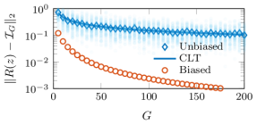
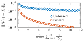
Figure 9: Resolvent approximation by sampling from a collection of Gaussian ancillary wavefunctions, for $z=-0.8+0.2i$ and the (scaled) MFIM Hamiltonian with $L_{\rm sys}=8$ spins. The approximation $\mathcal{I}_{G}(z)$ is computed using the unbiased ($\diamond$) and biased ($\circ$) estimator (Eq. 31 and Eq. 36 respectively) for a requested accuracy of $\epsilon=10^{-3}$. To obtain the success probabilities, a reference state $\ket{\phi}$ with $p_{0}=0.4$ and $p_{n}=\frac{1-p_{0}}{N-1}$ for $n\geq 1$ is considered. Left: Approximation error $\|R(z)-\mathcal{I}_{G}(z)\|_{2}$ as a function of the number of Gaussians $G$. For given $G$, the unbiased estimator is evaluated over a total of 100 trials (with each trial randomly drawing $G$ Gaussian variances from the mixing density $\rho_{\rm mix}$), while the biased estimator with prescribed Gaussian variances is constructed in a single trial. The error for the unbiased estimator is averaged over the 100 trials, with individual trials displayed in the background in light blue. The central limit scaling is represented as the solid line. Right: Approximation error as a function of the approximate quantum cost $\frac{1}{T^{\rm max}}\sum_{j=1}^{G}\frac{1}{P_{A_{j}}}$. The sum of the inverse probabilities is normalized by the maximal runtime $T^{\rm max}(\epsilon)$ in the discrete-time approach.

To demonstrate the continuous-time LCU approach, we perform the resolvent construction via two kinds of Gaussian approximations. We use the unbiased estimator from Eq. 31 as our benchmark. Additionally, we introduce a biased estimator with the following Gaussian wavefunctions,

$$iR(z_{k})\approx\frac{1}{b_{k}G}\sum_{j=1}^{G}\int_{-\infty}^{\infty}dq\,\varphi_{g}(q;\Gamma_{j})e^{-iH\lvert q\rvert},\quad\text{where }\Gamma_{j}=-\frac{2}{b_{k}^{2}}\log\frac{1+2(j-1)}{2G}.$$ (36)

That is, we also compile the resolvent by employing a simple sum of equally weighted Gaussians, each with a deterministically assigned width, as opposed to the stochastic continuous mixture from Eq. 31. The bias of this construction can be systematically reduced by increasing the number of Gaussians $G$.

Convergence as a function of number of Gaussians.

We evaluate the two Gaussian approximations for the complex pole $z=-0.8+0.2i$ in Fig. 9. The left panel shows the approximation error, $\lVert R(z)-\mathcal{I}_{G}\rVert_{2}$, as a function of the Gaussian number $G$, where $\mathcal{I}_{G}$ denotes an approximation of the exact integral representation with $G$ Gaussians. We notice that the onset of convergence occurs significantly earlier for the biased estimator, resulting in an efficient continuous-time approximation.

In the right panel of Fig. 9, we quantify the actual quantum cost using the sum of inverse success probabilities, $\sum_{j=1}^{G}\frac{1}{P_{A_{j}}}$, which characterizes the total number of unit-duration Hamiltonian simulations attempted on average to realize a $G$-Gaussian approximation. This metric can be interpreted as the continuous-time equivalent of the total simulation time. For direct comparison with the discrete-time quadrature approach, we normalize the inverse probability metric by the maximal simulation time $T^{\rm max}$ (c.f. Eq. 16) in the discrete-time setting for $\epsilon=10^{-3}$. Our empirical observation indicates that the biased Gaussian estimator requires a total simulation time similar to its discrete-time counterpart to achieve the requested accuracy, despite the higher cost of constructing an unbiased Gaussian estimator. Accordingly, the continuous-time approach may offer a distinct resource advantage due to the maximal simulation time always being unity. We comment that the success probabilities $P_{A_{j}}$ vary with the reference state $\ket{\phi}$ as reflected in Eq. 34. Although we have chosen a specific state $\ket{\phi}$ for illustration, the trend shown in Fig. 9 remains consistent across different choices of reference state.

4.3 Gaussian kernel for real poles

For a real pole, a continuous-time compilation for the Gaussian kernel can be efficiently designed with the deployment of two continuous-variable ancillae. We consider preparation of the ancillae,

$$\ket{0}_{c}=\int_{0}^{q^{\rm max}(2\epsilon)}dq\,\psi_{1}(q)\ket{q}\otimes\int_{-\infty}^{\infty}dy\,\psi_{2}(y)\ket{y},$$ (37)

in the uniform and Gaussian states $\psi_{1}(q)=\frac{1}{\sqrt{q^{\rm max}}}$ and $\psi_{2}(y)=\sqrt{\varphi_{g}(y;1)}$ (c.f. Eq. 29), with a truncation at the value $q^{\rm max}(2\epsilon)$, i.e., depending on $2\epsilon$ instead of $\epsilon$ (see Section A.2 for the definition of $q^{\rm max}$). The two-ancillae setup follows similar ideas as for complex poles but does not require Monte Carlo sampling of the Gaussian width. The general setup is outlined below.

Driven under a total Hamiltonian $\tilde{H}\mathrel{\mathop{\mathchar 58\relax}}=(H-a_{k})\otimes\hat{q}\otimes\hat{y}$, a real-time evolution of unit duration generates the composite state,

$$e^{-i\tilde{H}}\ket{\phi}\ket{0}_{c} =\int_{0}^{q^{\rm max}}dq\,\int_{-\infty}^{\infty}dy\,\psi_{1}(q)\psi_{2}(y)e^{iy(a_{k}-H)q}\ket{\phi}\ket{q}\ket{y},$$ (38)

$$=\frac{\sqrt{\pi}}{\sqrt{2}q^{\rm max}}R_{\epsilon}(z_{k})\ket{\phi}\ket{0}_{c}+\ket{\perp},$$ (39)

where the residual state $\ket{\perp}$ belongs to the kernel of the projector ${\rm Id}\otimes\ket{0}_{c}\bra{0}_{c}$ and,

$$R_{\epsilon}(z_{k})=\frac{1}{\pi}\int_{0}^{q^{\rm max}}dq\,\int_{-\infty}^{\infty}dy\,e^{-y^{2}/2}e^{iy(a_{k}-H)q}\approx R(z_{k}).$$ (40)

Therefore by post-selecting the $y$-ancilla, we can implement the action of the resolvent on any initial state $\ket{\phi}$, i.e., the normalized state $R_{\epsilon}(z_{k})\ket{\phi}/\lVert R_{\epsilon}(z_{k})\ket{\phi}\rVert_{2}$ that is $\mathcal{O}\left(\frac{\epsilon}{q^{\rm max}}\right)$-close to the target state. The success probability of a post-selection is,

$$P_{R(z_{k})}^{\epsilon} =\frac{\pi}{2(q^{\rm max})^{2}}\lVert R_{\epsilon}(z_{k})\ket{\phi}\rVert_{2}^{2}=\frac{\pi(a_{k}^{-})^{2}}{8}\bigg{[}\log\frac{1}{\epsilon a_{k}^{-}}\bigg{]}^{-1}\sum\limits_{n=0}^{N-1}\frac{p_{n}}{\mathinner{\!\left\lvert a_{k}-E_{n}\right\rvert}^{2}},$$ (41)

which varies with the initial state $\ket{\phi}$ and spectrum ${\rm spec}(H)$.

Though the uniform state $\psi_{1}(q)$ has a simple physical interpretation of a particle-on-a-ring wavefunction where the ring diameter is of $\mathcal{O}(q^{\rm max})$ [11], we note that an implementation using only Gaussian states can be adopted. Different from the stochastic implementation discussed in Section 4.1, here we construct a single, deterministic block-encoding of the resolvent by exploiting the following integral relation,

$$\int_{0}^{\infty}dq\,\int_{-\infty}^{\infty}dy\,e^{-y^{2}/2+iy(a_{k}-H)q}=\frac{1}{2}\int_{-\infty}^{\infty}dq\,e^{-q^{2}/2\Gamma_{0}}\int_{-\infty}^{\infty}dy\,e^{-y^{2}/2+iy(a_{k}-H)q}+\mathcal{O}(\pi\epsilon),$$

where we define the variance $\Gamma_{0}=\frac{1}{\epsilon(a_{k}^{-})^{3}}$ along the $q$ coordinate. That is, we initialize the ancillae in a product state of Gaussian wavefunctions in the variables $q$ and $y$,

$$\ket{0}_{c}=\int_{-\infty}^{\infty}dq\,\int_{-\infty}^{\infty}dy\,\sqrt{\varphi_{g}(q;\Gamma_{0})\varphi_{g}(y;1)}\ket{q}\ket{y}.$$ (42)

Evolving this state under the total Hamiltonian $\tilde{H}$ yields an approximation to the resolvent,

$$e^{-i\tilde{H}}\ket{\phi}\ket{0}_{c}=\frac{1}{\sqrt{\Gamma_{0}}}R_{\epsilon}(z_{k})\ket{\phi}\ket{0}_{c}+\ket{\perp},$$ (43)

where $\ket{\perp}$ labels the residual orthogonal to the Gaussian initial state. Post-selection on the $y$-ancilla implements the normalized state $R_{\epsilon}(z_{k})\ket{\phi}/\lVert R_{\epsilon}(z_{k})\ket{\phi}\rVert_{2}$ that is $\mathcal{O}\left(\frac{\epsilon}{\sqrt{\Gamma_{0}}}\right)$-close to the target state, therefore achieving an effective $(\sqrt{\Gamma_{0}},\mathbf{2},\epsilon)$-BE of the resolvent. This encoding comes with a success probability,

$$P_{R(z_{k})}^{\epsilon} =\frac{1}{\Gamma_{0}}\lVert R_{\epsilon}(z_{k})\ket{\phi}\rVert_{2}^{2}=\epsilon(a_{k}^{-})^{3}\sum\limits_{n=0}^{N-1}\frac{p_{n}}{\mathinner{\!\left\lvert a_{k}-E_{n}\right\rvert}^{2}},$$ (44)

which scales less favorably in $\epsilon$ compared to Eq. 41, despite the simpler ancillae preparation and loading.

4.4 Numerical experiment for real poles

We examine the continuous-time LCU construction for real poles by initializing two continuous-variable ancillae. We compare two initialization scenarios: first, a combination of a uniform and Gaussian state as described by Eq. 37, and alternatively, a purely Gaussian construction enabled by Eq. 42.

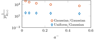
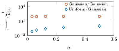
Figure 10: Cost necessary to construct an $\epsilon$-approximation to $(z-H)^{-1}$ with a requested accuracy $\epsilon=10^{-3}$. We consider the MFIM Hamiltonian with $L_{\rm sys}=8$ spins and $z=-1-2^{-k-1}$ for $k=0,1,\ldots,4$. The approximation is computed using two continuous-variable ancillae prepared in the uniform/Gaussian ($\diamond$) and Gaussian/Gaussian ($\circ$) initial states (Eq. 37 and Eq. 42) respectively. To obtain the success probability, a reference state $\ket{\phi}$ with $p_{0}=0.4$ and $p_{n}=\frac{1-p_{0}}{N-1}$ for $1\leq n\leq N-1$ is chosen. Left: The quantum cost $\frac{1}{P^{\epsilon}_{R(z)}}$ as a function of the pole position $a^{-}=\min_{n}\mathinner{\!\left\lvert a-E_{n}\right\rvert}$. Right: The relative cost, normalized by the maximal runtime $T^{\rm max}(\epsilon;z)$ in the discrete-time approach, as a function of the pole position.

We evaluate the two continuous-time approximations for the set of real poles $z_{k}=-1-2^{-1-k}$ in Fig. 10. In particular, we report the quantum cost $\frac{1}{P^{\epsilon}_{R(z_{k})}}$, understood as the number of unit-duration Hamiltonian simulations required on average to successfully realize an $\epsilon$-approximation. We consider a target accuracy of $\epsilon=10^{-3}$ as in Section 4.2. Notice that an approximation using the uniform-Gaussian initialization from Eq. 37 is significantly less expensive than using the purely Gaussian initialization from Eq. 42, although the latter is more practical to implement on hardware since Gaussian states are typically easier to manipulate. Eqs. 41 and 44 imply that the cost of approximating $R(z_{k})$ increases as $z_{k}$ moves closer to an eigenvalue. This pole dependence can be clearly visualized in the left pane. For the selected poles, we also compute the cost relative to the maximal runtime, $T^{\rm max}_{k}$, in the discrete-time setting. The normalized cost in the right pane in fact decreases as the pole approaches the Hamiltonian spectrum, exhibiting an opposite trend to that observed in Fig. 7 of Section 3.4. This suggests a slower cost growth relative to the discrete-time approach and highlights the resource efficiency of the continuous-time approach.

5 Construction of quantum rational transformations

In Sections 3 and 4, we have shown the construction of resolvents for varying pole locations and, additionally in Appendix B, the extension to multiple poles. These constructions allow for rational transformations on a quantum computer since any QRT can be written as a linear combination of resolvents, i.e.,

$$r(H;\bm{c},\bm{z},M)=\sum_{k=0}^{K-1}\sum_{m=1}^{M_{k}}c_{k,m}(z_{k}-H)^{-m}=\frac{\sum\limits_{d=0}^{M-1}\beta_{d}H^{d}}{\prod\limits_{k=0}^{K-1}(z_{k}-H)^{M_{k}}},$$ (45)

where $\bm{c}$, extending the single resolvent setting, is now the vector of coefficients $c_{k,m}$ associated with the poles $z_{k}$ accounting for their multiplicities $M_{k}$, and $(\beta_{0},\cdots,\beta_{M-1})$ defines polynomial coefficients in the numerator of the second equality, and $M=\sum_{k=0}^{K-1}M_{k}$ measures the total pole multiplicity. The rational function in Eq. 45 is said to be of degree $(M-1,M)$.

Efficient QRTs opens the path to the development of new quantum rational algorithms. Two emergent applications are spectral estimation and matrix function approximation. The latter can be tackled, e.g., using a contour integration approach [23] where the poles are placed on a customized contour. However, for some important functions, the poles for the optimal rational approximation are known and do not necessarily originate from a contour integral. We illustrate our efficient QRT construction for the signum function ${\rm sgn}\mathrel{\mathop{\mathchar 58\relax}}[-1,1]\rightarrow\{0,\pm 1\}$. Although the ${\rm sgn}(\omega)$ function appears simple, its discontinuity at $\omega=0$ poses a challenge for approximation. Polynomials cannot capture the discontinuity as accurately, thus making rational functions the preferred approximants.

A QRT approximating the matrix signum function is useful for computing the singular value decomposition and symmetric eigenvalue decomposition, as demonstrated by recent classical algorithms [38]. The ${\rm sgn}$ QRT can also be employed to construct a step function $\Theta(\omega)=\frac{1-{\rm sgn}(\omega)}{2}$ for filtering out high energy eigenstates in ground and excited state problems. Instead of relying on an idealized step filter, in practice we seek a rational approximant $r_{E}(\omega)\approx\Theta(\omega-E)$ so that,

$$\lvert r_{E}(E_{n})\rvert\approx\begin{cases}1&{\rm if}~{}E_{n}\leq E-\Delta E,\\ 0&{\rm if}~{}E_{n}\geq E+\Delta E,\end{cases}$$ (46)

where $\Delta E$ characterizes the width of the buffer region over which $\lvert r_{E}\rvert$ transitions roughly from $1$ to $0$. The width $\Delta E$ can be chosen to balance accuracy of the filter and its construction cost, since a smaller buffer width requires a higher degree rational approximant.

The Zolotarev rational functions, known for their abilities to approximate ${\rm sgn}(\omega)$ with a tight $L^{\infty}$ error bound, are introduced in Section 5.1. While a Zolotarev approximant does not follow from the contour integration approach, it can be generated with our proposed methods. We detail the quantum construction of the Zolotarev approximation through both discrete- and continuous-time LCU approaches. As the degree of the Zolotarev approximation increases, the poles tend to cluster towards the real line, which requires extended quantum resources (see 1). To mitigate the resource requirements, we take an iterative approach to construct a rational filter in Section 5.2, which is more efficient as we use poles further away from the real line.

5.1 Zolotarev approximation to ${\rm sgn}$

Zolotarev [1] provides a concrete expression for the $L^{\infty}$-optimal rational approximant of fixed degree to the sign function. For any given window $\mathcal{W}_{\overline{\omega}}=[-1,-\overline{\omega}]\cup[\overline{\omega},1]\subseteq[-1,1]$ with $\overline{\omega}>0$, the Zolotarev approximant, of degree $(2K-1,2K)$, is given by

$$r_{K}(\omega)=-\gamma_{K}\sum_{k=0}^{K-1}\left(\frac{c_{k}}{ib_{k}-\omega}+\frac{c_{k}}{-ib_{k}-\omega}\right),$$ (47)

where the poles $\pm ib_{k}$, residuals $c_{k}$, and multiplicative constant $\gamma_{K}$ are explicitly known [30]. The error of this approximant decays exponentially in the number of poles and can be bounded by

$${\rm err}_{K}\mathrel{\mathop{\mathchar 58\relax}}=\sup_{\omega\in\mathcal{W}_{\overline{\omega}}}\lvert r_{K}(\omega)-{\rm sgn}(\omega)\rvert\leq 4e^{-K\pi^{2}/2\log(4\overline{\omega})}.$$ (48)

See Appendix D for more details. In the following discussions, we examine the discrete-time and continuous-time LCU approaches for constructing the Zolotarev approximant.

5.1.1 Discrete-time LCU

To implement the Zolotarev approximant on the quantum computer, we observe that its action on a state $\ket{\phi}$ can be measured via the inner product,

$$\bra{\phi}r_{K}(H)\ket{\phi}=-i\left[\braket{\phi}{A}{\phi}-\braket{\phi}{A}{\phi}^{\ast}\right]=2\Im\braket{\phi}{A}{\phi},$$ (49)

where, for the Zolotarev poles $z_{k}=ib_{k}$ with $b_{k}\neq 0$,

$$A=-\gamma_{K}\sum_{k=0}^{K-1}c_{k}R(z_{k})=-\int_{0}^{\infty}dq\,c(q)e^{-iHq},\qquad c(q)=\gamma_{K}\sum_{k=0}^{K-1}c_{k}e^{-b_{k}q},$$ (50)

takes the form of an LCU. An efficient discrete-time LCU, implementing the $K$ relevant resolvents simultaneously, can be constructed with the quadrature technique discussed in Section 3.1. This is summarized in the following corollary.

Corollary 1.

For any given $\epsilon>0$, the Zolotarev signum approximant $r_{K}(H)$ admits a real-time LCU construction $r_{K,J}(H)$ with $\lVert r_{K}(H)-r_{K,J}(H)\rVert_{2}<\epsilon$. The Gauss-Legendre rule defines a time grid $\bm{t}$ such that

$$J=\log_{2}\log\frac{4\gamma_{K}}{\epsilon b^{-}}+(\eta+1)\log_{2}\frac{4\gamma_{K}}{\epsilon b^{-}}+3,$$ (51)

distinct time evolution circuits suffice to construct $r_{K,J}(H)$, where $\eta=\frac{3b^{-}-2\sqrt{2}b^{-}+\lVert H\rVert_{2}}{4\sqrt{2}b^{-}}$ and $b^{-}=\underset{0\leq k\leq K-1}{\min}b_{k}$. The maximal and total evolution time, respectively, can be controlled by

$$T^{\rm max}=\frac{1}{b^{-}}\log\frac{4\gamma_{K}}{\epsilon b^{-}},\quad\text{and}\quad T^{\rm tot}=\frac{J}{2b^{-}}\log\frac{4\gamma_{K}}{\epsilon b^{-}}.$$ (52)

Proof.

This follows from a direct application of 1 to $A$ in Eq. 50 together with the fact that $\sum_{k=0}^{K-1}c_{k}=1$. The expression of the total evolution time follows immediately from Eq. 51 and that of the maximal evolution time. ∎

We note that it suffices to consider the time grid $\bm{t}$ associated with the pole closest to the real line, $z^{-}=ib^{-}$. This finest time grid can be reused for other poles, allowing all quantum measurements to be combined classically during the postprocessing step. However, $z_{-}$ approaches the real axis as the degree of the rational approximant increases [1]. This could present a serious challenge for the discrete-time LCU due to the $\frac{1}{b^{-}}$ factor appearing in the maximal and total simulation times (cf. Eq. 52). The continuous-time LCU may alleviate this challenge via importance sampling in a stochastic implementation.

5.1.2 Continuous-time LCU

The continuous-time LCU construction of a Zolotarev approximant can be achieved via the Monte-Carlo strategy introduced in Sections 4.1 and 4.2. Since the coefficients $\{c_{k}\}_{k=0}^{K-1}$ from Eq. 47 satisfy the properties of a discrete probability measure, we acquire a Gaussian representation of $A$ that generalizes Eq. 31,

$$A =-\gamma_{K}\mathbb{E}_{K}\bigg{[}\frac{1}{b_{k}}\mathbb{E}_{\rm mix}\bigg{[}\int_{-\infty}^{\infty}dq\,\varphi_{g}(q;\Gamma)e^{-iH\lvert q\rvert}\bigg{]}\bigg{]}\approx-\frac{\gamma_{K}}{N_{K}}\sum_{\alpha=1}^{N_{K}}\frac{1}{b_{k_{\alpha}}G_{k_{\alpha}}}\sum_{\beta=1}^{G_{k_{\alpha}}}A_{\alpha\beta},$$ (53)

where $\mathbb{E}_{K}$ denotes an average over $[K]$ with respect to $\left\{c_{k}\right\}_{k=0}^{K-1}$ and

$$A_{\alpha\beta}=\int_{-\infty}^{\infty}dq\,\varphi_{g}(q;\Gamma_{\alpha\beta})e^{-iH\lvert q\rvert},$$ (54)

is a stochastic Zolotarev approximant that can be block-encoded by a continuous-variable ancilla. In Eq. 53, we sample Gaussian variance jointly from two probability distributions: $k_{\alpha}$ is sampled i.i.d. from the marginal distribution $\left\{c_{k}\right\}_{k=0}^{K-1}$ and $\Gamma_{\alpha\beta}$ i.i.d. from the conditional distribution $\rho_{\rm mix}(\cdot|b_{k_{\alpha}})$ defined in Eq. 30.

Recall that the cost of a continuous-time LCU scheme is determined by the Gaussian variance $\Gamma$ as a random variable. The Gaussian variance follows a distribution,

$$\rho_{K}(\Gamma)=\sum_{k=0}^{K-1}c_{k}\rho_{\rm mix}(\Gamma|b_{k}).$$ (55)

Due to the intimate connection between the Zolotarev parameters $(c_{k},b_{k})$ and the elliptic functions and integrals [1], we find that the average Gaussian width $\braket{\Gamma}_{K}\mathrel{\mathop{\mathchar 58\relax}}=\int_{0}^{\infty}d\Gamma\,\rho_{K}(\Gamma)\Gamma$ remains independent of $K$. Since the Gaussian width sets the spatial extent of continuous-variable wavefunction and thereby the ancilla preparation cost, this independence allows for the use of higher-degree rationals. To control the variance $\braket{\Gamma^{2}}_{K}-\braket{\Gamma}_{K}^{2}$, a practical approach involves employing a finite convex sum of Gaussians rather than a continuous mixture, as discussed within Section 4.2.

To illustrate the utility of the continuous-time approach, we perform a QRT that constructs the Zolotarev approximant $r_{K}$ for given rational degree $2K$ and buffer region width $2\overline{\omega}$. We follow the recipe of Eqs. 53 and 54 to generate a Monte-Carlo estimate $\hat{r}_{K}$ of $r_{K}$. To accelerate the convergence and control the sample variance, here we adopt the biased resolvent estimator using the Gaussian wavefunctions $\varphi_{g}(q;\Gamma_{j})$ with $\Gamma_{j}=-\frac{2}{b_{k}^{2}}\log\frac{1+2(j-1)}{2G_{k}}$ as in Eq. 36. For a given number $N_{\rm MC}$ of Monte-Carlo attempts, we then sample the Gaussian variance using two distributions, a marginal corresponding to the Zolotarev coefficients $\left\{c_{k}\right\}_{k}$ and a uniform conditional defined by Eq. 36. The bias of such a stochastic construction can be controlled by increasing the number of Gaussians $G_{k}$.

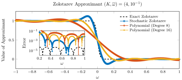
Figure 11: Rational and polynomial approximants of the step function $\Theta(\omega)$ over spectral region $[-1,1]$. The optimal Zolotarev approximant with $2K=8$ poles is indicated as the black dashed line while its stochastic construction via a continuous-time LCU is shown in blue. For comparison, the Chebyshev approximations of degrees $8$ and $16$, respectively, are colored in red and yellow. The inset displays the approximation error near the edge of the spectrum.

For $K=4$ and $G_{k}\equiv 8$, we display in Fig. 11 approximations of the step function $\Theta(H)$ by the exact Zolotarev QRT $r_{K}(H)$ and its stochastic implementation $\hat{r}_{K}(H)$ using $N_{\rm MC}=8$ Monte-Carlo samples. The same scaled Hamiltonian is considered as in Sections 3 and 4. Since $\lVert H\rVert_{2}\leq 1$, we simply examine values of the approximants over the spectral region $[-1,1]$. We note that the sampling procedure is purely classical, allowing for repeated trials to refine an optimal stochastic approximant. Empirically, the stochastic approximant $\hat{r}_{K}$ uniformly filters out eigenvalues of $H$ within $[2\overline{\omega},1]$. Moreover we show polynomial approximants of varying degrees in the Chebyshev basis. The rational approximations, in contrast to the polynomial counterparts, exhibit $(i)$ a sharper transition around $\omega=0$ and $(ii)$ a smaller error across $\mathcal{W}_{\overline{\omega}}=[-1,-\overline{\omega}]\cup[\overline{\omega},1]$. These distinctive features contribute to effective spectral filtering.

5.2 Efficient rational filtering by iterative function composition

The Zolotarev rational function can approximate the step function to a desired accuracy by increasing the number of poles. However, as these poles approach the real line, the cost of computing the corresponding resolvents becomes more expensive as indicated by 1. Alternatively, a fixed rational function (fixed number of poles) achieving a lower approximation accuracy can be applied iteratively and also obtain accurate eigenenergy approximations. Since the cost of resolvent simulation is fully determined by the distance $b_{k}$ of the pole $z_{k}=a_{k}+b_{k}i$ to the real line and by the distance of $a_{k}$ to the spectrum of the (filtered) Hamiltonian of interest, each iteration can be performed at a constant cost.

We assume knowledge of the spectral bounds, $E_{-}\leq E_{n}\leq E_{+}$, although the precise largest and smallest eigenenergies do not need to be known in advance. To achieve a reduction of spectral range $[E_{-},E_{+}]\mapsto[E_{-},E_{-}+\delta E]$ for arbitrary $\delta E$, we propose the repeated application of a fixed rational matrix filter $r_{E}(H)$ alternated by a shift and rescale of the resulting matrix. Suppose that applying $r_{E}(H)$ suppresses the eigenvalues in some interval $[E+\Delta E,E_{+}]$, thereby reducing the effective spectral range by a factor $\xi=\frac{E+\Delta E-E_{-}}{E_{+}-E_{-}}$. We define the following linear transformation, $f_{\xi}(\omega)=\frac{1}{\xi}(\omega-E_{-})+E_{-}$, which rescales the spectrum of $r_{E}(H)$ so that it is again approximately $[E_{-},E_{+}]$, allowing for the same filter $r_{E}$ to be applied again. For a given $\delta E$, this process can be repeated $D=\mathcal{O}(\log_{\xi}\delta E)$ times,

$$(r_{E}\circ f_{\xi^{D}})\cdots(r_{E}\circ f_{\xi^{3}})(r_{E}\circ f_{\xi^{2}})(r_{E}\circ f_{\xi})r_{E}(H)=\prod_{d=0}^{D}r_{E}\circ f_{\xi^{d}}(H)=\mathrel{\mathop{\mathchar 58\relax}}r_{\star D}(H;\xi),$$ (56)

which reduces the effective spectral range to $[E_{-},E_{-}+\delta E]$. For the discrete-time LCU approach, the efficiency of the iterative filtering process is captured by the corollary below.

Corollary 2.

A discrete-time $\epsilon$-approximation to the iterative filter constructed in Eq. 56, $\lVert r_{\star D}(H)-\sum_{j=0}^{J-1}x_{j}e^{-iHt_{j}}\rVert_{2}<\epsilon$ for $r_{E}(H)=\frac{1-r_{K}(H)}{2}$, can be obtained with

$$J=\log_{2}\log\frac{2(\gamma_{K})^{D}\mathcal{C}_{K}}{\epsilon\xi^{D}b^{-}}+\frac{3b^{-}+2\sqrt{2}b^{-}+\lVert H\rVert_{2}}{4\sqrt{2}b^{-}}\log_{2}\frac{2(\gamma_{K})^{D}\mathcal{C}_{K}}{\epsilon\xi^{D}b^{-}}+3,$$ (57)

distinct time evolution circuits and a maximum runtime of

$$T^{\rm max}=\frac{1}{\xi^{D}b^{-}}\log\frac{(\gamma_{K})^{D}\mathcal{C}_{K}}{\epsilon\xi^{D}b^{-}},$$ (58)

for $\gamma_{K}$ defined in Eq. 47 and a constant $\mathcal{C}_{K}$ dependent on the rational function $r_{K}$.

Proof.

The proof is provided in Section A.3. ∎

We note that the iterative rational filter $r_{\star D}$ can also be constructed using the continuous-time LCU approach discussed in Section 4. For a wide variety of many-body Hamiltonians $H$, the low-energy sector of the spectrum $\delta E$ is $\mathcal{O}(\frac{1}{{\rm polylog}N})$ relative to the spectral range. This results in $D=\log_{1/\xi}{\rm polylog}N$ iterations, where the cost of the filtering procedure is determined by the pole locations $\frac{b_{k}}{{\rm polylog}N}$ (the imaginary parts are scaled down by a factor of $\xi$ with each iteration).

6 Application of QRT to the ground and excited state problem

Once a quantum rational transformation is available, constructed via the discrete- or continuous time LCU approaches introduced in this paper, it can be employed in the context of the ground and excited state problem. For example, the QRT from Section 5 which implements an approximation to the step function can be used as a pre-processing routine for certain quantum eigensolvers to speed up their convergence. In Section 6.1 we describe how a QRT can be used as a pre-processing routine for the recently developed real-time approach for eigenenergy estimation, the observable dynamical mode decomposition (ODMD) [46]. We apply this approach to solve the ground and excited state problem in Section 6.2 for a TFIM Hamiltonian.

6.1 QRT for eigensolver acceleration

For a given Hamiltonian $H=\sum_{n=0}^{N-1}E_{n}\ket{E_{n}}\bra{E_{n}}$, an initial state $\ket{\psi}$, and a measurement state $\bra{\phi}$, ODMD measures the dynamical expectations,

$$o(\tau_{j})=\braket{\phi}{e^{-iH\tau_{j}}}{\psi}=\sum_{n=0}^{N-1}\tilde{p}_{n}e^{-iE_{n}\tau_{j}},\qquad\tau_{j}=j\Delta\tau,$$ (59)

on the quantum computer, these measurements allow us to identify a least-squares solution $B$ satisfying,

$$\begin{bmatrix}o(\tau_{1})&o(\tau_{2})&o(\tau_{3})&\cdots\\ o(\tau_{2})&o(\tau_{3})&o(\tau_{4})&\cdots\\ o(\tau_{3})&o(\tau_{4})&o(\tau_{5})&\cdots\\ \vdots&\vdots&\vdots&\ddots\end{bmatrix}\stackrel{{\scriptstyle{\rm LS}}}{{=}}B\begin{bmatrix}o(\tau_{0})&o(\tau_{1})&o(\tau_{2})&\cdots\\ o(\tau_{1})&o(\tau_{2})&o(\tau_{3})&\cdots\\ o(\tau_{2})&o(\tau_{3})&o(\tau_{4})&\cdots\\ \vdots&\vdots&\vdots&\ddots\end{bmatrix}.$$ (60)

The matrix $B$ is called the system matrix and contains the key frequency/energy information for advancing each observable vector a timestep $\Delta\tau$ forward. We sample over a relatively small number of timesteps so that $B$, upon a regularization, remains well-conditioned and compact in size. This makes classical diagonalization viable: the extremal eigenphase, $\tilde{E}_{0}=-\frac{1}{\Delta\tau}\max_{\lambda_{B}}{\rm arg}(\lambda_{B})$ for eigenvalues $\lambda_{B}$ of $B$, provides a reliable estimate of the exact ground state energy $E_{0}$.

By applying a suitable QRT $r(H)$ to the initial state $|\phi\rangle$, i.e., $r(H)\ket{\phi}$, we can improve the convergence of ODMD. This is inspired by adopting a signal processing perspective, Eq. 59 can be understood as sinusoidal data comprised of exponentially many components $e^{-iE_{n}\tau_{j}}$, each oscillating in time at its own frequency. The application of a rational filter $r(\omega)$ through a QRT can remove the high-energy components from $\ket{\psi}$. Then, applying ODMD leads to the measurement of the filtered expectations,

$$o_{\star}(\tau_{j})=\braket{\phi}{e^{-iH\tau_{j}}r(H)}{\psi}\approx\sum_{n=0}^{N_{c}}\tilde{p}_{n}e^{-iE_{n}\tau_{j}},$$ (61)

where $N_{c}$ is an eigenindex such that $E_{N_{c}}\lesssim E_{-}+\delta E\lesssim E_{N_{c}+1}$. The filtered expectations $o_{\star}$ can be computed with a sequence of time-evolution circuits as discussed in Section 5. Following the filtering procedure, we find a new system matrix $B_{\star}$ that effectively describes the dynamics within some low-energy subspace. Diagonalization of $B_{\star}$ thereby enables a simultaneous estimation of eigenenergies in this subspace.

6.2 Application to TFIM

We now apply our real-time rational framework to address the problem of finding the low-energy states of a many-body Hamiltonian, a significant task encountered within physical, chemical, and materials sciences. We illustrate the QRT pre-processing using the MFIM Hamiltonian in Eq. 17 with parameters $(h,g)=(0,1)$, so that we recover a transverse-field Ising model (TFIM) at the critical point, where the gap between the ground and first excited state closes in the thermodynamic limit. Our goal is to compute the $N_{c}=3$ lowest eigenenergies of a system with $L_{\rm sys}=12$ spins.

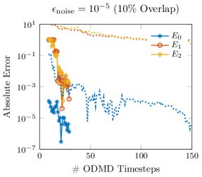
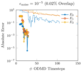
Figure 12: Absolute errors in the TFIM eigenenergies calculated as a function of the number of ODMD timesteps $\tau_{j}=j\Delta\tau$. Convergence of the $N_{c}=3$ lowest eigenenergies are shown both with (solid lines) and without (dashed lines) the application of the rational filter $r_{\star 3}(H)=(r_{E}\circ f_{\xi^{3}})(r_{E}\circ f_{\xi^{2}})(r_{E}\circ f_{\xi})r_{E}$. The rational filter is constructed iteratively from a base filter specified by $(K,E_{\pm},\Delta E)=(4,\pm 1,10^{-1})$ where $K$, $E_{\pm}$, and $\Delta E$ determine the rational degree, spectral bounds, and width of the filter buffer region. Left: ODMD algorithm run on noisy data with $(\epsilon_{\rm noise},p_{0})=(10^{-5},10^{-1})$ where $\epsilon_{\rm noise}$ and $p_{0}$ specify the noise level and ground state overlap. Right: ODMD algorithm run on noisy data with $(\epsilon_{\rm noise},p_{0})=(10^{-5},2\times 10^{-4})$. The singular value threshold parameter $\tilde{\delta}$ is adjusted for the filtered and unfiltered cases to ensure optimal performance.

For our eigenstate problem, as an illustration, we set $\ket{\psi}=\ket{\phi}$ with fixed ground state overlap $\tilde{p}_{0}=p_{0}=\lvert\braket{E_{0}}{\phi}\rvert^{2}$ and uniform excited state overlap $\tilde{p}_{n}=p_{n}=\frac{1-p_{0}}{2^{L_{\rm sys}}-1}$ for $n\geq 1$. To account for the effects of noise, we first compute the exact overlap matrix elements in Eqs. 59 and 61. We then introduce Gaussian perturbations $\mathcal{N}(0,\epsilon_{\rm noise}^{2})$ to the matrix elements. According to the central limit theorem, the Gaussian noise model can faithfully capture effects of the shot noise, i.e., the statistical errors due to taking a finite number of measurements. Some types of hardware noise may also be Gaussian; we do not investigate hardware noise models that specifically include decoherence or systematic errors. In order to classically mitigate the impact of noise, we employ singular value thresholding [46] to regularize the LS solution in Eq. 60. In particular, we truncate all singular values of the system matrix that are smaller than a set threshold $\tilde{\delta}\sigma_{\rm max}$ relative to the largest singular value $\sigma_{\rm max}$.

Fig. 12 shows the obtained approximations to the lowest three eigenenergies with different ground state overlap $p_{0}$. The dashed curves represent the ODMD results with $\ket{\psi}=|\phi\rangle$. For $p_{0}=10\%$, the approximation to the ground state energy $E_{0}$ converges rapidly to a reasonable accuracy of $\epsilon=10^{-3}$. Nevertheless, the approximations to the excited state energies $E_{1}$ and $E_{2}$ stagnate, highlighting the challenge in capturing these excited states. This issue is more pronounced for a poorer initial state with $p_{0}=0.02\%$, where none of the three energy approximations converge effectively. By applying a suitable rational filter $r(H)$ on the initial state $|\phi\rangle$, i.e., choosing $\ket{\psi}=r(H)\ket{\phi}$, and running the ODMD with this filtered state, the convergence improves significantly. This is illustrated by the solid curves in Fig. 12 with $r=r_{\star 3}$, i.e., $D=3$ in Eq. 80. Such an improvement in performance is evident even when $\ket{\phi}$ has uniform eigenstate overlap ($p_{0}=p_{n}\equiv 2^{-L_{\rm sys}}$ in the right panel). Thus, the application of a rational filter accelerates the simultaneous estimation of eigenenergies, especially for excited state energies where the convergence of regular ODMD becomes stagnant.

7 Conclusions

In this work, we investigate the capability of real-time evolution for implementing rational transformations on quantum hardware. Leveraging LCU as our algorithmic primitive, we focus on the effective construction of operator resolvents via Hamiltonian simulations. Specifically, we present two distinct and complementary LCU strategies that optimize the overall simulation cost. First, we consider a discrete-time scheme based on exponentially convergent quadrature rules. As a counterpart tailored for analog implementation, we also introduce a stochastic continuous-time scheme that employs resourceful bosonic ancillae. These two schemes provide a comprehensive toolkit for composing a rational function as a linear combination of resolvents.

Given the unique strength of rational functions in capturing singularities, we delve into the construction of optimal rational approximation of the signum function on a quantum computer. We demonstrate the application of rational transformations to the ground and excited state problem, where we build a spectral filter to extract the low-lying eigenenergies of a many-body system. As rational functions outperform polynomials by a landslide for a variety of central tasks in scientific computing, our framework offers novel insights into exploiting such advantage, for example universal function approximation, on the quantum platform.

8 Acknowledgements

This work was funded by the U.S. Department of Energy under Contract No. DE-AC02-05CH11231, through the Office of Science, Office of Advanced Scientific Computing Research (ASCR) Exploratory Research for Extreme-Scale Science. This research used resources of the National Energy Research Scientific Computing Center (NERSC), a U.S. Department of Energy Office of Science User Facility located at Lawrence Berkeley National Laboratory, operated under Contract No. DE-AC02-05CH11231. This work started during NVB’s research visit to Lawrence Berkeley National Laboratory, partially supported by Charles University Research program No. PRIMUS/21/SCI/009. The authors thank Siddharth Hariprakash for helpful discussions.

Appendix A Proofs

A.1 Theorem 1

Proof. By the triangle inequality, we have

$$\lVert R(z_{k})-\mathcal{I}_{J}(z_{k})\rVert_{2}\leq\lVert R(z_{k})-\mathcal{I}_{\infty}(z_{k})\rVert_{2}+\lVert\mathcal{I}_{\infty}(z_{k})-\mathcal{I}_{J}(z_{k})\rVert_{2},$$ (62)

where the two terms on the RHS represent the truncation and discretization errors, denoted as $\epsilon_{1}$ and $\epsilon-\epsilon_{1}$. By Eq. 12, we already know that $\lVert\bm{t}\rVert_{\infty}\leq\frac{1}{b_{k}}\log\frac{1}{\epsilon_{1}b_{k}}$. Moreover, the error bound of Eq. 14 clearly applies to the entire function $f_{n}(t)=e^{i(z_{k}-E_{n})T_{k}^{\rm max}(1+t)/2}$ where $E_{n}\in[-1,1]$ is the $n$th eigenvalue of $H$. It is rather straightforward to show through direct calculations that $\forall\sigma>1$,

$$\max_{0\leq n\leq N-1}\sup_{t\in\mathcal{E}_{\sigma}}\lvert f_{n}(t)\rvert\leq e^{[a_{k}^{+}(\sigma-\sigma^{-1})+b_{k}(\sigma-2+\sigma^{-1})]T_{k}^{\rm max}/4}.$$ (63)

This supremum estimate implies an overall error estimate (cf. Eqs. 12 and 14),

$$\lVert R(z_{k})-\mathcal{I}_{J}(z_{k})\rVert_{2}\leq\epsilon_{1}+\frac{4\sigma^{2-2J}}{(\sigma^{2}-1)b_{k}}\left(\frac{1}{\epsilon_{1}b_{k}}\right)^{\eta_{k}}\log\frac{1}{\epsilon_{1}b_{k}},$$ (64)

where

$$\eta_{k}(\sigma)=\frac{(\sigma-1)^{2}b_{k}+(\sigma^{2}-1)a_{k}^{+}}{4\sigma b_{k}}$$ (65)

appears as an exponent. Therefore Eq. 64 implies that

$$J(\epsilon,\epsilon_{1})=\frac{1}{2}\log_{\sigma}\log\frac{1}{\epsilon_{1}b_{k}}+\frac{\eta_{k}}{2}\log_{\sigma}\frac{1}{\epsilon_{1}b_{k}}+\frac{1}{2}\log_{\sigma}\frac{4}{(\sigma^{2}-1)(\epsilon-\epsilon_{1})b_{k}}+1$$ (66)

Legendre nodes suffice for an $\epsilon$-accurate approximation. By setting, for example, $\sigma=\sqrt{2}$ and $\epsilon_{1}=\frac{\epsilon}{2}$, we arrive at the upper bound as claimed. We conclude our proof by noting that the Gauss-Legendre time grid $\bm{t}$ is symmetric around $0$: the center of symmetry shifts to $\frac{T_{k}^{\rm max}}{2}$ after we revert the change of variable. ∎

A.2 Theorem 2

Proof. Again by the triangle inequality, we have

$$\lVert R(z_{k})-\mathcal{I}_{J}(z_{k})\rVert_{2}\leq\lVert R(z_{k})-\mathcal{I}_{\infty}(z_{k})\rVert_{2}+\lVert\mathcal{I}_{\infty}(z_{k})-\mathcal{I}_{J}(z_{k})\rVert_{2},$$ (67)

where the truncation and approximation errors contain contributions from both the Gauss-Legendre and trapezoidal rules. For $T_{k}^{\rm max}=\lVert\bm{t}\rVert_{\infty}=q^{\rm max}y^{\rm max}$, observe that

$$\lVert R(z_{k})-\mathcal{I}_{\infty}(z_{k})\rVert_{2}\leq\frac{1}{a_{k}^{-}}{\rm erfc}\bigg{(}\frac{a_{k}^{-}q^{\rm max}}{2}\bigg{)}+\frac{\sqrt{2}q^{\rm max}}{\sqrt{\pi}}{\rm erfc}\left(\frac{y^{\rm max}}{\sqrt{2}}\right),$$ (68)

where the RHS involving the complementary error function ${\rm erfc}(\cdot)$ accounts for truncation error along the $q$ and $y$ coordinate respectively. Given $0<\epsilon_{1}<\epsilon$ sufficiently small, setting $q^{\rm max}=\frac{2}{a_{k}^{-}}\sqrt{\log\frac{2}{\epsilon_{1}a_{k}^{-}}}$ and $y^{\rm max}=\sqrt{2\log\frac{2}{\epsilon_{1}a_{k}^{-}}}$ yields

$$\lVert R(z_{k})-\mathcal{I}_{\infty}(z_{k})\rVert_{2}\leq\bigg{[}\frac{1}{a_{k}^{-}}+\frac{2\sqrt{2}}{\pi a_{k}^{-}}\bigg{]}\frac{\epsilon_{1}a_{k}^{-}}{2}<\epsilon_{1},$$ (69)

where we invoke simple bounds, such as a Chernoff-type upper bound ${\rm erfc}(x)\leq\frac{1}{\sqrt{\pi}x}e^{-x^{2}}$, to obtain an estimate of the truncation error.

For the approximation error, we can apply the bound of Eq. 20 to the entire function $F_{n}(y|q)=e^{-y^{2}/2}e^{iy(a_{k}-E_{n})q}$. Direct calculations show that $\forall\sigma_{y}>0$,

$$\max_{0\leq n\leq N-1}e_{\Delta y}[F_{n}(\cdot|q)]\lesssim 2\sqrt{2\pi}e^{\sigma_{y}^{2}/2+\sigma_{y}a_{k}^{+}\lvert q\rvert-2\pi\sigma_{y}/\Delta y},$$ (70)

for a trapezoidal step $\Delta y=\frac{2y^{\rm max}}{L_{y}-1}$ and given $q$ coordinate. The supremum estimate implies an approximation error,

$$\begin{split}\lVert\mathcal{I}_{\infty}(z_{k})-\mathcal{I}_{J}(z_{k})\rVert_{2}\leq\frac{1}{\pi}\int_{0}^{q^{\rm max}}&dq\,\max_{0\leq n\leq N-1}e_{\Delta y}[F_{n}(\cdot|q);\mathcal{S}_{\sigma_{y}}]\\ &+\frac{q^{\rm max}\Delta y}{2\pi}\sum_{\ell=0}^{L_{y}-1}e^{-y_{\ell}^{2}/2}\max_{0\leq n\leq N-1}e_{L_{q}}[f_{n\ell};\mathcal{E}_{\sigma_{q}}],\end{split}$$ (71)

where $f_{n\ell}(q)=e^{iy_{\ell}(a_{k}-E_{n})q^{\rm max}(1+q)/2}$ denotes the integrand in Eq. 9, now transformed to the interval $[-1,1]$, and $L_{q}$ the number of discretization nodes for the Gauss-Legendre rule. The terms $e_{\Delta y}[F_{n}(\cdot|q)]$ and $e_{L_{q}}[f_{n\ell}]$ capture discretization errors associated with the trapezoidal and Legendre rule respectively, derived in relation to region of analyticity $\mathcal{S}_{\sigma_{y}}$ and $\mathcal{E}_{\sigma_{q}}$. Setting $\sigma_{y}=y^{\rm max}$ and $\sigma_{q}=\sqrt{2}$ for simplicity, we hence arrive at an estimate of the overall error,

$$\begin{split}\lVert R(z_{k})-\mathcal{I}_{J}(z_{k})\rVert_{2}\leq\epsilon_{1}+\frac{4\sqrt{2}}{\sqrt{\pi}\epsilon_{1}a_{k}^{+}a_{k}^{-}y^{\rm max}}&e^{-\pi(L_{y}-1)}\bigg{[}\frac{2}{\epsilon_{1}a_{k}^{-}}\bigg{]}^{4\sqrt{2}\zeta_{k}}\\ &+\frac{\sqrt{2}2^{5-L_{q}}}{\pi a^{-}_{k}}\bigg{[}\frac{2}{\epsilon_{1}a_{k}^{-}}\bigg{]}^{\zeta_{k}}\log\frac{2}{\epsilon_{1}a_{k}^{-}},\end{split}$$ (72)

where the exponent reads $\zeta_{k}=\frac{a_{k}^{+}}{2a_{k}^{-}}$. We can separately control the second and third term within arbitrary small tolerance $\epsilon_{2}$ and $\epsilon_{3}$, i.e., taking

$$L_{y}(\epsilon_{1},\epsilon_{2})=\frac{1}{\pi}\bigg{[}\log\frac{4e^{\pi}}{\sqrt{\pi}\epsilon_{1}\epsilon_{2}a_{k}^{+}a_{k}^{-}}-\frac{1}{2}\log\log\frac{2}{\epsilon_{1}a_{k}^{-}}+4\sqrt{2}\zeta_{k}\log\frac{2}{\epsilon_{1}a_{k}^{-}}\bigg{]},$$ (73)

and

$$L_{q}(\epsilon_{1},\epsilon_{3})=\log_{2}\frac{32\sqrt{2}}{\pi\epsilon_{3}a^{-}_{k}}+\zeta_{k}\log_{2}\frac{2}{\epsilon_{1}a_{k}^{-}}+\log_{2}\log\frac{2}{\epsilon_{1}a_{k}^{-}},$$ (74)

suffices to obtain an $\epsilon$-accurate approximation. The total number of discretization nodes is $J(\epsilon_{1},\epsilon_{2},\epsilon_{3})=L_{y}L_{q}$. Further setting $\epsilon_{1}=2\epsilon_{2}=2\epsilon_{3}=\frac{\epsilon}{2}$, we recover the upper bound as claimed. ∎

A.3 Corollary 2

Before giving the proof to 2, we need the following property.

Property 1.

The application of $D$ iterations, as in Eq. 56, requires computation of $(D+1)K$ resolvents.

Proof of 1. According to Eq. 56, the application of $D$ iterations immediately implies the need to compute $K^{D+1}$ resolvents. For a rational filter of the form $r_{E}(H)=\sum_{k=0}^{K-1}c_{k}R(z_{k})+{\rm h.c.}$ (where ${\rm h.c.}$ denotes the Hermitian conjugate), we have,

$$(r_{E}\circ f_{\xi})(H)=\sum_{k=0}^{K-1}\xi c_{k}R(f_{1/\xi}(z_{k}))+{\rm h.c.},$$ (75)

where the resolvent identity [57] implies,

$$[(r_{E}\circ f_{\xi})r_{E}](H) =\sum_{k,k^{\prime}=0}^{K-1}\sum_{\iota,\iota^{\prime}=\pm}\xi c_{k\iota}c_{k^{\prime}\iota^{\prime}}R(f_{1/\xi}(z_{k\iota}))R(z_{k^{\prime}\iota^{\prime}}),$$ (76)

$$=\sum_{k,k^{\prime}=0}^{K-1}\sum_{\iota,\iota^{\prime}=\pm}\frac{\xi c_{k\iota}c_{k^{\prime}\iota^{\prime}}}{\tilde{z}_{k^{\prime}\iota^{\prime}}-\xi\tilde{z}_{k\iota}}\left[R(f_{1/\xi}(z_{k\iota}))-R(z_{k^{\prime}\iota^{\prime}})\right],$$ (77)

with $c_{k\pm}=\Re c_{k}\pm i\Im c_{k}$, $z_{k\pm}=a_{k}\pm ib_{k}$, and $\tilde{z}_{k\pm}=z_{k\pm}-E_{-}$. For simplicity, we introduce the subscript $\iota$ to designate the complex conjugation of a scalar or the Hermitian conjugation of an operator. The composed filter $r_{\star 1}(H;\xi)=[(r_{E}\circ f_{\xi})r_{E}](H)$ acts on an initial state $\ket{\phi}$ as

$$\begin{split}\braket{\phi}{f(H)r_{\star 1}(H;\xi)}{\phi}=\xi\sum_{k=0}^{K-1}\sum_{\iota=\pm}&c_{k\iota}^{(1)}(\xi)\braket{\phi}{f_{\iota}(H)R(f_{1/\xi}(z_{k}))}{\phi}_{\iota}\\ &+\sum_{k=0}^{K-1}\sum_{\iota=\pm}c^{(1)}_{k\iota}(1/\xi)\braket{\phi}{f_{\iota}(H)R(z_{k})}{\phi}_{\iota},\end{split}$$ (78)

where

$$c_{k\iota}^{(1)}(\xi)=\sum_{k^{\prime}=0}^{K-1}\sum_{\iota^{\prime}=\pm}\frac{c_{k\iota}c_{k^{\prime}\iota^{\prime}}}{\tilde{z}_{k^{\prime}\iota^{\prime}}-\xi\tilde{z}_{k\iota}}.$$ (79)

That is, we have converted the evaluation of $K^{2}$ resolvent products (c.f. Eq. 76) to that of $2K$ resolvents within a single iterative filtering step. From a recursive argument it follows immediately that Eq. 56 can, therefore, be constructed by only $D(K+1)$ resolvents. ∎

Proof of 2. An efficient rational approximation to the step function can be obtained by the Zolotarev approximant $r_{K}(H)$ in Eq. 47, i.e., $r_{E}(H)=\frac{1-r_{K}(H)}{2}$. Below we describe in detail a discrete-time procedure for constructing the corresponding iterative filter $r_{\star D}(H)$. First observe that

$$r_{\star D}(H;\xi)=\frac{1}{2^{D+1}}\sum_{d=0}^{D+1}(-1)^{d}\sum_{\bm{s}\subseteq[D+1]\mathrel{\mathop{\mathchar 58\relax}}\lvert\bm{s}\rvert=d}\prod_{i=0}^{d-1}r_{K}\circ f_{\xi^{s_{i}}}(H),$$ (80)

where each $\bm{s}=[s_{0},s_{1},\cdots,s_{d-1}]$ is a multi-index specified by distinct $s_{i}\in[D+1]$. We simply assume that $\bm{s}$ is ordered with $s_{i}<s_{i+1}$. Thus to construct a discrete-time filter $\epsilon$-close to $r_{\star D}(H)$, it suffices to adopt a Legendre rule $\bm{t}$ such that

$$\bigg{\lVert}\prod_{i=0}^{d-1}r_{K}\circ f_{\xi^{s_{i}}}(H)-\sum_{j=0}^{J-1}x_{j}e^{-iHt_{j}}\bigg{\rVert}_{2}\leq\epsilon,$$ (81)

for all multi-indices $\bm{s}$. We assert that $\bm{s}=[D+1]$ incurs the largest error among multi-indices since by 1,

$$J_{\bm{s}}=\log_{2}\log\frac{2(\gamma_{K})^{d}\lVert\bm{c}_{\bm{s}}\rVert_{1}}{\epsilon\xi^{\lVert\bm{s}\rVert_{\infty}}b^{-}}+\frac{3b^{-}+2\sqrt{2}b^{-}+\lVert H\rVert_{2}}{4\sqrt{2}b^{-}}\log_{2}\frac{2(\gamma_{K})^{d}\lVert\bm{c}_{\bm{s}}\rVert_{1}}{\epsilon\xi^{\lVert\bm{s}\rVert_{\infty}}b^{-}}+3,$$ (82)

and

$$\lVert\bm{t}_{\bm{s}}\rVert_{\infty}=\frac{1}{\xi^{\lVert\bm{s}\rVert_{\infty}}b^{-}}\log\frac{(\gamma_{K})^{d}\lVert\bm{c}_{\bm{s}}\rVert_{1}}{\epsilon\xi^{\lVert\bm{s}\rVert_{\infty}}b^{-}},$$ (83)

where $\bm{c}_{\bm{s}}$ is the vector of rational coefficients satisfying

$$\prod_{i=0}^{d-1}r_{K}\circ f_{\xi^{s_{i}}}(H)=(-\gamma_{K})^{d}\sum_{i=0}^{d-1}\sum_{k=0}^{K-1}\sum_{\iota=\pm}(c_{\bm{s}})_{ik\iota}R(f_{1/\xi^{s_{i}}}(z_{k\iota})),$$ (84)

with $\lVert\bm{c}_{\bm{s}}\rVert_{1}$ bounded by $\xi^{\lVert\bm{s}\rVert_{\infty}}$. We notice that the spectral transformation $H\mapsto f_{\xi}(H)$ does not stretch the effective Hamiltonian spectral range, since we apply the transformed filters in a sequential way. For example, an application of the initial filter $r_{K}(H)$ almost ‘eliminates’ the components of $\ket{\phi}$ in the energy range $[E+\Delta E,E_{+}]$, which also holds during succeeding iterative steps that operate on a smaller and smaller effective spectral range. ∎

Appendix B Extension from simple to repeated poles

The real-time constructions in Section Sections 3 and 4 can be generalized to account for a pole of higher multiplicity, thus extending our analysis beyond a simple pole associated with the resolvent. A natural generalization is to consider the $m^{\rm th}$-power of a resolvent $R^{m}(z_{k})=(z_{k}-H)^{-m}$ for any positive integer $m$. Notably, a higher-order pole can be expressed through time evolutions if we simply differentiate Eq. 3,

$$(z_{k}-H)^{-m} =\frac{(-1)^{m-1}}{(m-1)!}\frac{d^{m-1}}{d\omega^{m-1}}(z_{k}+\omega-H)^{-1}\bigg{\rvert}_{\omega=0},$$ (85)

$$=\frac{(-i)^{m-1}}{(m-1)!}\int_{0}^{\infty}dq\,q^{m-1}\int_{-\infty}^{\infty}dy\,y^{m-1}\Lambda_{k}(y)e^{iy(z_{k}-H)q},$$ (86)

where Eq. 85 holds by functional calculus [57]. Observe that the polynomial growth of $q^{m-1}$ or $y^{m-1}$ in the integrand is dominated by the exponential decay of $\Lambda_{k}e^{-iy(z_{k}-H)q}$.

For discrete-time LCU, the observation above implies that the maximal evolution time, at the leading order, remains the same as in the case of a simple pole. For continuous-time LCU, we can block-encode $R^{m}(z_{k})$ stochastically with Gaussian states when $b_{k}>0$, i.e.,

$$\begin{split}R^{m}(z_{k})=\frac{(-i)^{m}}{(m-1)!}\int_{0}^{\infty}&dq\,q^{m-1}e^{-b_{k}q+i(a_{k}-H)q}\\ &\approx\frac{(-i)^{m}}{(m-1)!}\sum_{j=1}^{G}\int_{-\infty}^{\infty}dq\,\varphi_{g}(q;q_{j},\Gamma_{j})e^{i(a_{k}-H)q},\end{split}$$ (87)

where $q^{m-1}e^{-b_{k}q}$ follows the density of a gamma distribution with shape parameter $m$ and rate parameter $b_{k}$, and we invoke Gaussian mixture approximation detailed in Section 4 now with a set of center-displaced Gaussians $\varphi_{g}(q;q_{j},\Gamma_{j})\mathrel{\mathop{\mathchar 58\relax}}=\varphi_{g}(q-q_{j},\Gamma_{j})$. In the large $m$ limit, the approximation holds for a single Gaussian mode by the central limit theorem, since a gamma random variable is statistically identical to the sum of $m$ i.i.d. exponential variables. When $b_{k}=0$, we can block-encode $R^{m}(z_{k})$ deterministically with two bosonic excited states,

$$R^{m}(z_{k})\approx\frac{C}{2}\int_{-\infty}^{\infty}dq\,\psi_{m}^{2}(q;\Gamma^{{\rm max},m})\int_{-\infty}^{\infty}dy\,\psi_{m}^{2}(y;1)e^{iy(a_{k}-H)q},$$ (88)

where $\psi_{m}(q;\Gamma^{{\rm max},m})$, for instance, is the $m^{\rm th}$-lowest eigenstate of the harmonic oscillator with a characteristic width $\sqrt{\Gamma^{{\rm max},m}}$, and $C$ is a normalization constant. Therefore the overall cost of implementing higher-order resolvent is marginally affected by pole multiplicity.

Appendix C Numerical benchmark for the Heisenberg models

Using the 2D and 3D Heisenberg spin Hamiltonians on different lattices, we run more experiments illustrating the main findings in this paper. All Hamiltonians considered are taken from the HamLib collection [45], where more details on the Hamiltonians can be found.

For the Hamiltonian "2D triag pbc qubitnodes Lx=4, Ly=6, h=2" with a pole located at $z=-0.49+0.1i$, Fig. 13 shows the convergence of the quadrature rules described in Section 3.1. The results confirm the conclusion in Section 3.2: the Legendre shows fast exponential convergence, outperforming the trapezoidal and Laguerre rule.

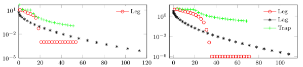
Figure 13: Error $\|R(z)-\mathcal{I_{J}}(z)\|_{2}$ shown as a function of the scaled total evolution time $\frac{\|\bm{t}\|_{1}}{T^{\rm max}}$, for $z=-0.49+0.1i$ and the (scaled) Hamlib Hamiltonian "2D triag pbc qubitnodes Lx=4, Ly=6, h=2" of size $2^{12}\times 2^{12}$. The approximation $\mathcal{I_{J}}(z)$ is computed using the trapezoidal (+), Legendre ($\circ$) and Laguerre ($\ast$) rule for a requested accuracy $\epsilon=10^{-3}$ (left) and $\epsilon=10^{-6}$ (right).

We perform the same experiment for different Hamiltonians and pole locations, where the Legendre rule similarly requires a lower cost for the approximation of the resolvent. The considered Hamlib Hamiltonians are:

• "2D-triag-pbc-qubitnodes Lx-3 Ly-5 h-2" ($z$=-0.49+0.1i and $z$=0+0.1i)

• "3D-grid-pbc-qubitnodes Lx-2 Ly-2 Lz-2 h-2" ($z$=-0.71+0.1i)

Appendix D Zolotarev rational approximant

The Zolotarev rational approximant in Eq. 47 achieves a favorable error that is asymptotically sharp with respect to the supremum norm,

$${\rm err}_{K}=\sup_{\omega\in\mathcal{W}_{\overline{\omega}}}\lvert r_{K}(\omega)-{\rm sgn}(\omega)\rvert=\frac{2\sqrt{Z_{K}}}{1+Z_{K}},$$ (89)

where $Z_{K}(\overline{\omega})$, known as the Zolotarev number, depends on the approximation region set by $\overline{\omega}$ and can be bounded by $0\leq Z_{K}\leq 4e^{-K\pi^{2}/\log(4\overline{\omega})}$ [5]. This implies an exponentially decaying error ${\rm err}_{K}\leq 4e^{-K\pi^{2}/2\log(4\overline{\omega})}$, also reported in Eq. 48. We remark that a tighter bound can be derived in terms of the Grötzsch ring function (see [5]).

The Zolotarev number enjoys the important invariance property that

$$Z_{K}(\mathcal{W}_{\overline{\omega}})\equiv Z_{K}(\mathcal{T}([-1,-\overline{\omega}])\cup\mathcal{T}([\overline{\omega},1])),$$ (90)

for any Möbius transformation $\mathcal{T}$. Such invariance allows us to restrict to windows of the previous form. This is because for any pair of disjoint, ordered intervals $[\omega_{a},\omega_{b}]\cup[\omega_{c},\omega_{d}]$, we can identify a Möbius transformation $\mathcal{T}_{abcd}$ such that

$$\mathcal{T}_{abcd}([\omega_{a},\omega_{b}])=[-1,-\overline{\omega}],\qquad\mathcal{T}_{abcd}([\omega_{c},\omega_{d}])=[\overline{\omega},1],$$ (91)

where the transformed window bound $\overline{\omega}$ satisfies

$$\frac{(1+\overline{\omega})^{2}}{4\overline{\omega}}=\frac{(\omega_{c}-\omega_{a})(\omega_{d}-\omega_{b})}{(\omega_{c}-\omega_{b})(\omega_{d}-\omega_{a})}=\frac{(\omega_{ab}+\omega_{bc})(\omega_{bc}+\omega_{cd})}{\omega_{bc}(\omega_{ab}+\omega_{bc}+\omega_{cd})},$$ (92)

with, for example, $\omega_{ab}\mathrel{\mathop{\mathchar 58\relax}}=\omega_{b}-\omega_{a}$ (so a larger value of $\omega_{bc}$, i.e., larger buffer width $\Delta E$ in Eq. 46, results in a faster convergence).

References

- [1] N. I. Akhiezer, Elements of the theory of elliptic functions, vol. 79, American Mathematical Soc., 1990.
- [2] U. L. Andersen, J. S. Neergaard-Nielsen, P. van Loock, and A. Furusawa, Hybrid discrete- and continuous-variable quantum information, Nature Physics, 11 (2015), pp. 713–719.
- [3] A. C. Antoulas, C. A. Beattie, and S. Güğercin, Interpolatory Methods for Model Reduction, Society for Industrial and Applied Mathematics, Philadelphia, PA, 2020.
- [4] W. E. Arnoldi, The principle of minimized iterations in the solution of the matrix eigenvalue problem, Quarterly of Applied Mathematics, 9 (1951), pp. 17–29.
- [5] B. Beckermann and A. Townsend, On the singular values of matrices with displacement structure, SIAM Journal on Matrix Analysis and Applications, 38 (2017), pp. 1227–1248.
- [6] D. Berry and L. Novo, Corrected quantum walk for optimal Hamiltonian simulation, Quantum Information and Computation, 16 (2016), p. 1295–1317.
- [7] D. W. Berry, G. Ahokas, R. Cleve, and B. C. Sanders, Efficient quantum algorithms for simulating sparse Hamiltonians, Communications in Mathematical Physics, 270 (2007), pp. 359–371.
- [8] D. W. Berry, A. M. Childs, R. Cleve, R. Kothari, and R. D. Somma, Simulating Hamiltonian dynamics with a truncated Taylor series, Physical Review Letters, 114 (2015), p. 090502.
- [9] D. W. Berry, D. Motlagh, G. Pantaleoni, and N. Wiebe, Doubling the efficiency of hamiltonian simulation via generalized quantum signal processing, Physical Review A, 110 (2024), p. 012612.
- [10] D. Camps, K. Meerbergen, and R. Vandebril, An implicit filter for rational Krylov using core transformations, Linear Algebra and Its Applications, 561 (2019), pp. 113 – 140.
- [11] S. Chakraborty, Implementing any linear combination of unitaries on intermediate-term quantum computers, arXiv preprint arXiv:2302.13555, (2023).
- [12] A. M. Childs, On the relationship between continuous- and discrete-time quantum walk, Communications in Mathematical Physics, 294 (2010), pp. 581–603.
- [13] A. M. Childs, R. Kothari, and R. D. Somma, Quantum algorithm for systems of linear equations with exponentially improved dependence on precision, SIAM Journal on Computing, 46 (2017), pp. 1920–1950.
- [14] A. M. Childs and N. Wiebe, Hamiltonian simulation using linear combinations of unitary operations, Quantum Information and Computation, 12 (2012), p. 901–924.
- [15] P. J. Davis and P. Rabinowitz, Methods of numerical integration, Computer science and applied mathematics, Academic Press, San Diego, 2nd ed. ed., 1984.
- [16] Y. Dong, L. Lin, and Y. Tong, Ground-state preparation and energy estimation on early fault-tolerant quantum computers via quantum eigenvalue transformation of unitary matrices, PRX Quantum, 3 (2022), p. 040305.
- [17] V. Druskin and L. Knizhnerman, Extended Krylov subspaces: Approximation of the matrix square root and related functions, SIAM Journal on Matrix Analysis and Applications, 19 (1998), pp. 755–771.
- [18] G. A. Evans, Some new thoughts on Gauss–Laguerre quadrature, International Journal of Computer Mathematics, 82 (2005), pp. 721–730.
- [19] Y. Futamura, X. Ye, and T. Sakurai, Contour integral-based quantum algorithm for estimating matrix eigenvalue density, arXiv preprint arXiv:2112.05395, (2021).
- [20] H. C. J. Gan, G. Maslennikov, K.-W. Tseng, C. Nguyen, and D. Matsukevich, Hybrid quantum computing with conditional beam splitter gate in trapped ion system, Phys. Rev. Lett., 124 (2020), p. 170502.
- [21] W. Gautschi, A survey of gauss-christoffel quadrature formulae, in E. B. Christoffel: The Influence of His Work on Mathematics and the Physical Sciences, P. L. Butzer and F. Fehér, eds., Basel, 1981, Birkhäuser Verlag, pp. 72–147.
- [22] A. Gilyén, Y. Su, G. H. Low, and N. Wiebe, Quantum singular value transformation and beyond: exponential improvements for quantum matrix arithmetics, in Proceedings of the 51st Annual ACM SIGACT Symposium on Theory of Computing, STOC 2019, New York, NY, USA, 2019, Association for Computing Machinery, p. 193–204.
- [23] N. J. Higham, Functions of Matrices, Society for Industrial and Applied Mathematics, Philiadelphia, 2008.
- [24] M. Hochbruck and C. Lubich, On Krylov subspace approximations to the matrix exponential operator, SIAM Journal on Numerical Analysis, 34 (1997), pp. 1911–1925.
- [25] T. Keen, E. Dumitrescu, and Y. Wang, Quantum algorithms for ground-state preparation and Green’s function calculation, arXiv preprint arXiv:2112.05731, (2021).
- [26] W. Kirby, M. Motta, and A. Mezzacapo, Exact and efficient Lanczos method on a quantum computer, Quantum, 7 (2023), p. 1018.
- [27] K. Klymko, C. Mejuto-Zaera, S. J. Cotton, F. Wudarski, M. Urbanek, D. Hait, M. Head-Gordon, K. B. Whaley, J. Moussa, N. Wiebe, W. A. de Jong, and N. M. Tubman, Real-time evolution for ultracompact Hamiltonian eigenstates on quantum hardware, PRX Quantum, 3 (2022), p. 020323.
- [28] G. Kurizki, P. Bertet, Y. Kubo, K. Mølmer, D. Petrosyan, P. Rabl, and J. Schmiedmayer, Quantum technologies with hybrid systems, Proceedings of the National Academy of Sciences, 112 (2015), pp. 3866–3873.
- [29] C. Lanczos, An iteration method for the solution of the eigenvalue problem of linear differential and integral operators, Journal of Research of the National Bureau of Standards, 45 (1950), pp. 255–282.
- [30] Y. Li and H. Yang, Interior eigensolver for sparse Hermitian definite matrices based on Zolotarev’s functions, Communications in Mathematical Sciences, 19 (2021), pp. 1113–1135.
- [31] Y. Liu, S. Singh, K. C. Smith, E. Crane, J. M. Martyn, A. Eickbusch, A. Schuckert, R. D. Li, J. Sinanan-Singh, M. B. Soley, T. Tsunoda, I. L. Chuang, N. Wiebe, and S. M. Girvin, Hybrid oscillator-qubit quantum processors: Instruction set architectures, abstract machine models, and applications, 2024.
- [32] S. Lloyd, Universal quantum simulators, Science, 273 (1996), pp. 1073–1078.
- [33] G. H. Low and I. L. Chuang, Optimal Hamiltonian simulation by quantum signal processing, Physical Review Letters, 118 (2017), p. 010501.
- [34] , Hamiltonian Simulation by Qubitization, Quantum, 3 (2019), p. 163.
- [35] D. Lubinsky, Geometric convergence of Lagrangian interpolation and numerical integration rules over unbounded contours and intervals, Journal of Approximation Theory, 39 (1983), pp. 338–360.
- [36] J. M. Martyn, Z. M. Rossi, A. K. Tan, and I. L. Chuang, Grand unification of quantum algorithms, PRX Quantum, 2 (2021), p. 040203.
- [37] M. Motta, C. Sun, A. T. Tan, M. J. O’Rourke, E. Ye, A. J. Minnich, F. G. Brandão, and G. K.-L. Chan, Determining eigenstates and thermal states on a quantum computer using quantum imaginary time evolution, Nature Physics, 16 (2020), pp. 205–210.
- [38] Y. Nakatsukasa and R. W. Freund, Computing fundamental matrix decompositions accurately via the matrix sign function in two iterations: The power of Zolotarev’s functions, SIAM Review, 58 (2016), pp. 461–493.
- [39] Y. Nakatsukasa, O. Sète, and L. N. Trefethen, The AAA algorithm for rational approximation, SIAM Journal on Scientific Computing, 40 (2018), pp. A1494–A1522.
- [40] D. J. Newman, Rational approximation to , Michigan Mathematical Journal, 11 (1964), pp. 11 – 14.
- [41] M. A. Nielsen and I. L. Chuang, Quantum Computation and Quantum Information: 10th Anniversary Edition, Cambridge University Press, 2010.
- [42] T. Park and G. Casella, The Bayesian lasso, Journal of the American Statistical Association, 103 (2008), pp. 681–686.
- [43] J.-M. Pirkkalainen, S. U. Cho, J. Li, G. S. Paraoanu, P. J. Hakonen, and M. A. Sillanpää, Hybrid circuit cavity quantum electrodynamics with a micromechanical resonator, Nature, 494 (2013), pp. 211–215.
- [44] A. Ruhe, Rational Krylov sequence methods for eigenvalue computation, Linear Algebra and its Applications, 58 (1984), pp. 391–405.
- [45] N. P. Sawaya, D. Marti-Dafcik, Y. Ho, D. P. Tabor, D. E. B. Neira, A. B. Magann, S. Premfaratne, P. Dubey, A. Matsuura, N. Bishop, W. A. de Jong, S. Benjamin, O. D. Parekh, N. Tubman, K. Klymko, and D. Camps, HamLib: A library of Hamiltonians for benchmarking quantum algorithms and hardware, arXiv preprint arXiv:2306.13126, (2024).
- [46] Y. Shen, D. Camps, A. Szasz, S. Darbha, K. Klymko, D. B. Williams-Young, N. M. Tubman, and R. V. Beeumen, Estimating eigenenergies from quantum dynamics: A unified noise-resilient measurement-driven approach, arXiv preprint arXiv:2306.01858, (2023).
- [47] T. Souichi, O. Asuka, S. Tomohiro, and T. S. Usuda, Quantum algorithm for matrix functions by Cauchy’s integral formula, Quantum Information and Computation, 20 (2020), p. 14–36.
- [48] , Quantum algorithms based on the block-encoding framework for matrix functions by contour integrals, Quantum Information and Computation, 22 (2022), pp. 965–979.
- [49] G. Szegő, Orthogonal Polynomials, vol. 23 of Americal Mathematical Society Colloquium Publications, American Mathematical Society, Providence, RI, 4th ed., 1975.
- [50] Y. Tong, D. An, N. Wiebe, and L. Lin, Fast inversion, preconditioned quantum linear system solvers, fast Green’s-function computation, and fast evaluation of matrix functions, Physical Review A, 104 (2021), p. 032422.
- [51] L. N. Trefethen, Approximation Theory and Approximation Practice, Extended Edition, Society for Industrial and Applied Mathematics, Philadelphia, PA, 2019.
- [52] L. N. Trefethen and J. A. C. Weideman, The exponentially convergent trapezoidal rule, SIAM Review, 56 (2014), pp. 385–458.
- [53] R. Van Beeumen, K. Meerbergen, and W. Michiels, Compact rational Krylov methods for nonlinear eigenvalue problems, SIAM Journal on Matrix Analysis and Applications, 36 (2015), pp. 820–838.
- [54] B. von Sydow, Error estimates for Gaussian quadrature formulae, Numerische Mathematik, 29 (1977/1978), pp. 59–64.
- [55] A. Wallraff, D. I. Schuster, A. Blais, L. Frunzio, R.-. S. Huang, J. Majer, S. Kumar, S. M. Girvin, and R. J. Schoelkopf, Strong coupling of a single photon to a superconducting qubit using circuit quantum electrodynamics, Nature, 431 (2004), pp. 162–167.
- [56] Y. Wang, H. Xiang, and S. Zhang, Quantum algorithm for matrix logarithm by integral formula, Quantum Information Processing, 22 (2023), p. 76.
- [57] K. Yosida, Functional Analysis, Springer, Berlin, Heidelberg, 6th ed., 1995.