A discrete-time survival model to handle interval-censored covariates

Abstract

Methods are lacking to handle the problem of survival analysis in the presence of an interval-censored covariate, specifically the case in which the conditional hazard of the primary event of interest depends on the occurrence of a secondary event, the observation time of which is subject to interval censoring. We propose and study a flexible class of discrete-time parametric survival models that handle the censoring problem through joint modeling of the interval-censored secondary event, the outcome, and the censoring mechanism. We apply this model to the research question that motivated the methodology, estimating the effect of HIV status on all-cause mortality in a prospective cohort study in South Africa.
Keywords: discrete survival model, interval-censored covariate, HIV serostatus

1 Introduction

Survival data, also known as time-to-event data, are ubiquitous in public health research and require specialized methods to handle event times that may not be observed directly, but are instead subject to censoring. Typically, the censored event time is the outcome of interest in an analysis, such as mortality or the onset of a disease. However, in certain situations we may also have a censored covariate (the secondary event), related to the outcome (the primary event) in the sense that at any point in time, the conditional hazard of the primary event depends on whether the secondary event has occurred.

In particular, we focus on the case in which the outcome of interest is right-censored and a covariate is interval-censored. With interval censoring, the value of a covariate $X$ is not known exactly, but is known to lie within an interval $[l,u]$. This definition is broad, and includes right-censoring (in which $u=\infty$ and $X\geq l$), left-censoring (in which $l=-\infty$ and $X\leq u$), and what we refer to as “finite interval censoring” (in which $l$ and $u$ are both finite and in the interior of the support of $X$) as special cases. Furthermore, missing data can be thought of as a case of interval-censoring in which $l=-\infty$ and $u=\infty$. Thus, the framework of interval censoring is broad and applicable to a wide variety of settings.

A vast body of research has been developed for handling right-censored outcomes, including classical methods such as the Kaplan-Meier estimator(Kaplan and Meier, 1958) and the Cox proportional hazards model (Cox, 1972). Additionally, a number of methods are available for when the outcome variable is interval-censored (see, for example, Lindsey and Ryan, 1998, Kor et al., 2013, Pan and Chappell, 2002), including the case when the censoring mechanism is informative (Finkelstein et al., 2002); see Gómez et al. (2009) for a review. However, relatively little work has been done to handle situations in which covariates are right-censored or interval-censored; the setting of a survival model in the presence of an interval-censored covariate is the focus of this paper.

This work is motivated by the problem of estimating the effects of HIV serostatus (the interval-censored covariate) on downstream outcomes, such as all-cause mortality or occurrence of a stroke. With the transition of the global HIV epidemic from a routinely fatal disease to a chronic disease with increasing life expectancy, there is growing interest in measuring the effects of chronic HIV infection and its treatment on risk of non-communicable diseases and non-AIDS mortality. Numerous longitudinal cohort studies, initially designed to estimate the epidemiology of HIV incidence or shorter-term AIDS related complications, have expanded focus to include study of non-AIDS complications and longer-term mortality (D’Souza et al., 2021, Gange et al., 2007, Reniers et al., 2016). To do so, there is a requirement to comprehensively classify the HIV serostatus of all individuals in these cohorts, including those who are initially observed as HIV uninfected. Ideally, population-based studies would include routine and updated HIV testing data on all individuals (e.g. annually) to enable such classification. However, in reality, most population-based studies have episodic HIV testing data, which includes individuals who lack HIV testing data, irregular HIV testing schedules, and sizeable populations of individuals who have a final HIV test years before chronic disease and mortality outcomes. Individuals in these types of studies fall into one of four categories: (1) those who have a negative HIV test followed by a positive test, (2) those whose most recent test was negative, (3) those whose first test was positive, and (4) those who have never received a test. With respect to the date of seroconversion, these four cases correspond to finite interval censoring, right-censoring, left-censoring, and missing data, respectively. A method that can handle all four types of interval censoring simultaneously would enable new lines of research, including estimating the impact of policy decisions on HIV-related outcomes at the population level, and determining causes of morbidity and mortality for which the HIV+ population is at increased risk. An example of the former is determining how the large-scale transition from efavirenz-based to dolutegravir-based first-line ART impacted morbidity and mortality for people living with HIV. An example of the latter is determining whether HIV status is associated with increased risk of stroke, diabetes, hypertension, and other non-communicable diseases.

In terms of related works, we identified seven papers that deal with interval-censored covariates in the context of a survival model. Lee et al. (2003) and Atem et al. (2019) consider an adaptation to the Cox proportional hazards model to a setting in which both the outcome and a covariate are right-censored, and Sattar et al. (2012) consider a similar setting in which the covariate is instead left-censored and propose a full parametric model. However, none of these methods are appropriate for an interval-censored covariate. The remaining four papers consider an interval-censored covariate. Goggins et al. (1999) considers a survival data setting similar to our own in which one covariate (the status of a binary event process, measured through periodic tests) is interval censored. They take an approach that involves an EM algorithm with a Gibbs sampling E-step; although this setting is similar to our own, the proposed method is computationally impractical for large datasets, and the imputation of the event process is not allowed to depend on individual-level covariates, a major limitation. Langohr et al. (2004) consider HIV status as an interval-censored exposure in a survival model, but the simple log-linear parametric model they propose is too inflexible for our setting (e.g., it does not allow for time-varying covariates) and the distribution of the interval-censored variable is similarly not allowed to depend on individual-level covariates. Tian and Lagakos (2006) consider a survival setting in which a binary covariate process is observed at a single time point; their method is useful but not applicable in our setting where individuals may have zero, one, or multiple measurements of the covariate process. The setting of Ahn et al. (2018) is similar to ours, and they consider three possible modifications to a Cox model. However, their estimators are mainly useful for settings in which the covariate is known to lie between two time points, as they essentially discard all information from person-time intervals following the last observation of the covariate process.

The contribution of this work is to propose and study a flexible class of parametric discrete-time survival models that are computationally tractable when applied to large datasets that involve an interval-censored covariate and time-varying covariates. This class of models is broad, and allows for both the conditional hazard of the secondary event and the censoring mechanism to depend on covariates. To our knowledge, this is the only work to study a discrete-time survival model with an interval-censored covariate.

The organization of the remainder of this paper is as follows. In Section 2, we introduce the data structure and describe our statistical model. In Section 3, we conduct a simulation study to evaluate the operating characteristics of our model and confirm code functionality. In section 4, we demonstrate the use of our model through application to a dataset from a large HIV cohort in South Africa. In Section 5, we summarize findings, limitations, and future research directions.

2 Methods

2.1 Data structure, ideal model, and parameters of interest

We begin by describing an ideal data structure that involves no censoring or missingness, and then use this structure to describe the data we observe in reality. Suppose that we have a (possibly open) longitudinal cohort of individuals, indexed by $i\in\{1,...,n\}$, with observations occurring within an observation window defined by calendar time, which is discretized into intervals indexed by $j\in\{1,...,J\}$. For each individual, we have observations corresponding to some subset $(s_{i},s_{i}+1,...,t_{i})\subset(1,2,...,J)$, which we refer to as the observation interval for that individual. The start time $s_{i}$ corresponds to either the start date of the observation window ($s_{i}=1$) or the time at which the subject enters the risk set. The end time $t_{i}$ represents either the time at which the outcome of interest occurred, the end of the observation window, or the time at which the subject exits the risk set. For an individual $i$ at time $j\in(s_{i},s_{i}+1,...,t_{i})$, we observe an outcome indicator $Y_{i,j}$, a fully-observed covariate vector $Z_{i,j}$, and an indicator $X_{i,j}$ representing whether a secondary event has occurred (where in reality $X_{i,j}$ may be missing). For ease of exposition, we assume that $X_{i,j}$ is univariate (i.e., there is only one secondary event); in Section 5, we discuss possible extensions to handling multivariate $X_{i,j}$. We also assume that for each individual, the outcome can only occur once, and that observation stops for that individual once it has occurred. Also let $X_{i}\equiv(X_{i,s_{i}},X_{i,s_{i}+1},...,X_{i,t_{i}})$ and $X\equiv(X_{1},X_{2},...,X_{n})$, and define $Y_{i}$, $Z_{i}$, $Y$, and $Z$ analogously.

For each individual, we assume that the data follow a longitudinal process in which two Markov-type assumptions hold. First, we assume that the probability (discrete hazard) of the secondary event $X_{i,j}$ occurring at time $j$ depends only on the fully observed covariates $Z_{i,j}$ at time $j$, and does not depend at all on the outcome history. Formally, this can be written as

$$P(X_{i,j}\,|\,\bar{X}_{i,j-1},\bar{Y}_{i,j-1},\bar{Z}_{i,j})=P(X_{i,j}\,|\,Z_{i,j},X_{i,j-1}=0)\,,$$ (1)

where $\bar{Z}_{i,t}\equiv(Z_{i,s_{i}},Z_{i,s_{i}+1},...,Z_{i,t})$ represents the covariate history of $Z$ up to time $t$, and analogous definitions hold for $\bar{X}_{i,t}$ and $\bar{Y}_{i,t}$. Second, we assume that the probability (discrete hazard) of the outcome occurring at time $j$ depends only on whether or not it occurred at time $j-1$ and the covariates (including the secondary event process) at time $j$. This can be written as

$$P(Y_{i,j}=y\,|\,\bar{X}_{i,j},\bar{Y}_{i,j-1},\bar{Z}_{i,j})=P(Y_{i,j}=y\,|\,X_{i,j},Y_{i,j-1},Z_{i,j})\,.$$ (2)

Note that both probabilities are allowed to depend on study time $j$. Next, we define $p_{x}^{*}$ as

$$p_{x}^{*}(\tilde{x},z,j,s,\Omega)\equiv P(X_{i,j}=1\,|\,X_{i,j-1}=\tilde{x},Z_{i,j}=z,j,I(j=s_{i})=s,\Omega)\,,$$

the conditional probability that the secondary event has occurred by time $j$ given $(X_{i,j-1},Z_{i,j},I(j=s_{i}))$. Note that $p_{x}^{*}(\tilde{x}=1,z,j,s,\Omega)=1$ for all $(z,j,s,\Omega)$ and that $p_{x}^{*}(\tilde{x}=0,z,j,s,\Omega)$ is a discrete hazard function. Also note that $X_{i,s_{i}-1}$ is undefined, and a model for $p_{x}^{*}$ must account for this “initial status”; this is the reason for conditioning on $I(j=s_{i})$, an indicator that the current observation is the first for individual $i$. We also denote by $p_{y}^{*}(x,z,j,\Omega)$ the discrete hazard (probability) of the outcome occurring in time interval $j$ given $(X_{i,j}=x,Z_{i,j}=z,\Omega)$; that is,

$$p_{y}^{*}(x,z,j,\Omega)\equiv P(Y_{i,j}=1\,|\,Y_{i,j-1}=0,X_{i,j}=x,Z_{i,j}=z,j,\Omega)\,,$$

The corresponding conditional probability mass functions (PMFs) are given by

$$f_{x}^{*}(x\,|\,\tilde{x},z,j,s,\Omega) \equiv\{p_{x}^{*}(\tilde{x},z,j,s,\Omega)\}^{x}\{1-p_{x}^{*}(\tilde{x},z,j,s,\Omega)\}^{1-x}\,,$$

$$f_{y}^{*}(y\,|\,x,z,j,\Omega) \equiv\{p_{y}^{*}(x,z,j,\Omega)\}^{y}\{1-p_{y}^{*}(x,z,j,\Omega)\}^{1-y}\,.$$

We assume that interest lies in contrasts or parameters related to the discrete hazard function $p_{y}^{*}$. For example, if we assume that $p_{y}^{*}(x,z,j,\Omega)=\mathcal{C}^{-1}(\alpha^{\prime}x+\beta^{\prime}z+b(j))$, where $\mathcal{C}\mathrel{\mathop{\ordinarycolon}}x\mapsto\log\{-\log(1-x)\}$ is the complementary log-log link function, $\mathcal{C}^{-1}$ is its inverse, and $b(j)$ is an arbitrary function of calendar time, then the (exponentiated) parameters $\alpha$ and $\beta$ can be interpreted as hazard ratios (Prentice and Gloeckler, 1978). Conditions (1) and (2) allow us to write the joint PMF of $(X_{i},Y_{i})$ evaluated at the vector $(x,y)\equiv(x_{s_{i}},...,x_{t_{i}},y_{s_{i}},...,y_{t_{i}})$ given $Z_{i}=z\equiv(z_{s_{i}},...,z_{t_{i}})$ and $\Omega$ as

$$f_{x,y}(x,y\,|\,z,\Omega)\equiv\prod_{j={s_{i}}}^{t_{i}}f_{x}^{*}(x_{j}\,|\,x_{j-1},z_{j},j,I(j=s_{i}),\Omega)f_{y}^{*}(y_{j}\,|\,x_{j},z_{j},j,\Omega)\,.$$

2.2 Handling the interval-censored covariate process

If it were the case that $X$ was fully-observed, inference for $\Omega$ could be based on the log likelihood

$$\tilde{\ell}_{x,y}(\Omega|X,Y,Z) =\sum_{i=1}^{n}\log\left\{f_{x,y}(X_{i},Y_{i}\,|\,Z_{i},\Omega)\right\}$$

$$=\sum_{i=1}^{n}\sum_{j={s_{i}}}^{t_{i}}\log\left\{f_{x}^{*}(X_{i,j}\,|\,X_{i,j-1},Z_{i,j},j,I(j=s_{i}),\Omega)f_{y}^{*}(Y_{i,j}\,|\,X_{i,j},Z_{i,j},j,\Omega)\right\}\,,$$

However, in our case, $X$ is partially or completely interval-censored. Instead of observing $X_{i,j}$, we observe $U_{i,j}\equiv\Delta_{i,j}X_{i,j}$, where $\Delta_{i,j}$ is a binary variable that equals one if $X_{i,j}$ is known and zero otherwise and where here and elsewhere we use the simple notation $A=BC$ to represent the Hadamard (element-wise) product of the vectors $B$ and $C$ (as opposed to the matrix product $B^{\prime}C$). We proceed by (1) positing a mechanism or model for the missingness indicator $\Delta$, (2) deriving the form of the joint PMF of $(X,Y,\Delta,U\,|\,Z,\Omega)$, and (3) integrating out $X$ to derive the joint PMF of $(Y,\Delta,U\,|\,Z,\Omega)$, on which inference can be based.

For the first step, the joint PMF of $(X_{i},Y_{i},\Delta_{i})$ given $(Z_{i},\Omega)$ for an individual can be written as

$$f_{x,y,\delta}(x,y,\delta\,|\,z,\Omega)=f_{x,y}(x,y\,|\,z,\Omega)f_{\delta}(\delta\,|\,x,y,z,\Omega)\,,$$

where $f_{\delta}$ represents the PMF of the vector $\Delta_{i}$ conditional on $(X_{i},Y_{i},Z_{i},\Omega)$, the form of which is chosen by the user based on context. Assumptions about the missingness mechanism are implicitly encoded by the form of $f_{\delta}$; for example, if we assume that $X$ is missing at random, $f_{\delta}$ would not depend on $x$. For the second step, we note that since $U$ equals the product of $X$ and $\Delta$, we can write the conditional PMF of $(U_{i},X_{i},Y_{i},\Delta_{i})$ given $(Z_{i},\Omega)$ as

$$f_{u,x,y,\delta}(u,x,y,\delta\,|\,z,\Omega)=f_{x,y,\delta}(x,y,\delta\,|\,z,\Omega)I(u=x\delta)\,.$$

For the third step, we can obtain the conditional PMF of $(U_{i},Y_{i},\Delta_{i})$ given $(Z_{i},\Omega)$ as

$$f_{u,y,\delta}(u,y,\delta\,|\,z,\Omega)=\sum_{x\in\mathcal{X}}f_{u,x,y,\delta}(u,x,y,\delta\,|\,z,\Omega)\,,$$ (3)

where $\mathcal{X}$ is the support of $X_{i}$. Since $X_{i}$ will always equal a binary vector of the form $(0,...,0,1,...,1)$ (possibly with only zeros or only ones), the set $\mathcal{X}$ can be written as $\mathcal{X}\equiv\{R_{0}(k),(R_{0}(k-1),R_{1}(1)),...,(R_{0}(1),R_{1}(k-1)),R_{1}(k)\}$, where $k$ is the length of $X_{i}$, $R_{0}(n)$ represents a vector of $n$ zeros, and $R_{1}(n)$ represents a vector of $n$ ones. The resulting conditional log-likelihood function across all individuals is given by

$$\ell_{u,y,\delta}(\Omega|U,Y,\Delta,Z)=\sum_{i=1}^{n}\log\left\{f_{u,y,\delta}(U_{i},Y_{i},\Delta_{i}\,|\,Z_{i},\Omega)\right\}\,.$$ (4)

While $X$ is not observed for everyone, the quantity $U$ is always observed, and so inference for $\Omega$ can be based on (4). In most applications, the log-likelihood will have to be maximized numerically to compute estimators $\widehat{\Omega}$ and $\widehat{\text{Var}}(\widehat{\Omega})$ of $\Omega$ and $\text{Var}(\hat{\Omega})$, respectively.

2.3 Specification of model components

The form of the log-likelihood given in (4) requires specification of parametric forms for the functions $p_{x}^{*}$, $p_{y}^{*}$, and $f_{\delta}$. For the discrete hazard function $p_{y}^{*}$, a traditional approach is to use a linear predictor with a complementary log-log link function. This is a discrete analog of a Cox model for continuous-time data, and so the resulting parameters can be interpreted as hazard ratios (Prentice and Gloeckler, 1978). For example, we may have that

$$p_{y}^{*}(x,z,j,\Omega)=\mathcal{C}^{-1}\left\{\alpha_{y}+\beta x+\gamma_{y}^{\prime}z+\tau_{y}^{\prime}b_{y}(j)\right\}\,,$$ (5)

where again $\mathcal{C}^{-1}$ is the inverse of the complementary log-log link function and where $b_{y}$ is a vector-valued basis function (e.g., a natural cubic spline basis) modeling the calendar time trend. For the conditional distribution of the interval-censored variable $X$, a number of models are possible depending and one should be chosen based on context. In the motivating example for this work, the interval-censored covariate is HIV serostatus, a binary vector of the form $(0,...,0,1,...,1)$, with the change from $0$ to $1$ occurring at the point of seroconversion. One choice is to model this as

$$\begin{split}p_{x}^{*}(\tilde{x},z,j,s,\Omega)&\equiv\left[\tilde{\mathcal{C}}^{-1}\left\{\alpha_{s}+\gamma_{s}^{\prime}z+\tau_{s}^{\prime}b_{s}(j)\right\}\right]^{s}\\ &\qquad\times\left[\tilde{x}+(1-\tilde{x})\,\tilde{\mathcal{C}}^{-1}\left\{\alpha_{x}+\gamma_{x}^{\prime}z+\tau_{x}^{\prime}b_{x}(j)\right\}\,,\right]^{1-s}\,,\end{split}$$ (6)

where the notation $\tilde{\mathcal{C}}$ is used to emphasize that a different link function can be used if desired. Note that the form given in (6) includes two components: a parametric form for the “initial status model” (i.e., the conditional probability that the event has already happened for individual $i$ by the time of the first measurement $j=s_{i}$) and a separate parametric form for the “secondary event discrete hazard model” (i.e., for subsequent measurements at times $j>s_{i}$, the conditional probability of the event happening in one time interval given that it has not happened up to that point).

The function $f_{\delta}$ can be used to model the conditional interval censoring mechanism. Different forms are possible, but it will often be the case that measurements of the secondary event will be taken at specific points in time that inform knowledge of the event process at other points in time. In these cases, it is often more convenient to think of $\Delta_{i,j}$ as bivariate, given by $\Delta_{i,j}\equiv(\Delta_{i,j}^{\circ},\Delta_{i,j}^{*})$, where $\Delta_{i,j}^{\circ}$ represents whether $X_{i,j}$ is known (as before) and $\Delta_{i,j}^{*}$ is an indicator that equals one if a test or measurement for individual $i$ was taken at time $j$. Then, we can model the random variable $\Delta^{*}$ and use this variable to deterministically infer $\Delta^{\circ}$. For example, with HIV testing, if an individual is only tested once at time $t^{*}$, then it will be the case that $\Delta_{i,j}^{*}=1$ for $j=t^{*}$ and $\Delta_{i,j}^{*}=0$ for $j\neq t^{*}$. However, if the test is negative, then we know the event has not occurred at any time prior to $t^{*}$, and so we have that $\Delta_{i,j}^{\circ}=1$ for $j\leq t^{*}$ and $\Delta_{i,j}^{\circ}=0$ for $j>t^{*}$. This can be represented by defining a conditional PMF function for $\Delta_{i,j}^{*}$; for example, if we assume this variable depends on the covariate vector $Z_{i,j}$, we may specify the form

$$f_{\delta^{*}}(\delta^{*}\,|\,z,\Omega)\equiv\prod_{j=s_{i}}^{t_{i}}\left\{\tilde{\mathcal{C}}^{-1}(\alpha_{\delta}+\gamma_{\delta}^{\prime}z_{j}+\tau_{\delta}^{\prime}b_{\delta^{*}}(j))\right\}^{\delta_{j}^{*}}\left\{1-\tilde{\mathcal{C}}^{-1}(\alpha_{\delta}+\gamma_{\delta}^{\prime}z_{j}+\tau_{\delta}^{\prime}b_{\delta^{*}}(j))\right\}^{1-\delta_{j}^{*}}\,.$$ (7)

We can then write

$$f_{\delta}(\delta\,|\,x,y,z,\Omega)\equiv I\{\delta^{\circ}=g_{\delta}(x,\delta^{*})\}f_{\delta^{*}}(\delta^{*}\,|\,z,\Omega)\,,$$

where the function $g_{\delta}$ computes the vector $\Delta_{i}^{\circ}$ as a function of the vector $\Delta_{i}^{*}$ of testing times and the true event indicators $X_{i}$. In the context of our motivating HIV example, this function encodes the idea that (1) HIV status is known to be negative for all times prior to a negative test, and (2) HIV status is known to be positive for all times following a positive test. To give a form for this function, we first define a categorical variable $M_{i}$ that subdivides the population into four mutually exclusive and exhaustive groups. Group 1 consists of individuals who have no testing data whatsoever. Group 2 consists of individuals who have only ever received negative tests. Group 3 consists of individuals who received one or more negative tests followed by a positive test. Group 4 consists of individuals whose first and only test was positive. Mathematically, this is summarized through the following function, where $x$ and $\delta^{*}$ are both vectors of length $J$.

$$m(x,\delta^{*})\equiv\begin{cases}1,&\text{if}\ \sum_{j=1}^{J}\delta_{j}^{*}=0\,,\\ 2,&\text{if}\ \sum_{j=1}^{J}\delta_{j}^{*}>0,\sum_{j=1}^{J}\delta_{j}^{*}x_{j}=0\,,\\ 3,&\text{if}\ \sum_{j=1}^{J}\delta_{j}^{*}>0,\sum_{j=1}^{J}\delta_{j}^{*}x_{j}=1,\sum_{j=1}^{J}\delta_{j}^{*}(1-x_{j})>0\,,\\ 4,&\text{if}\ \sum_{j=1}^{J}\delta_{j}^{*}=1,\sum_{j=1}^{J}\delta_{j}^{*}x_{j}=1\,.\end{cases}$$

Using this definition, for each individual $i$, let $M_{i}\equiv m(X_{i},\Delta_{i}^{*})$. Also let $T_{i}^{-}\in\{1,2,...,J\}$ denote the index of the most recent negative test (defined for groups 2 and 3) and let $T_{i}^{+}\in\{1,2,...,J\}$ denote the index of the (only) positive test (defined for groups 3 and 4); these can be formally defined as $T_{i}^{-}\equiv t^{-}(X_{i},\Delta_{i}^{*})$ and $T_{i}^{+}\equiv t^{+}(X_{i},\Delta_{i}^{*})$, where

$$t^{-}(x,\delta^{*}) \equiv\operatorname*{arg\,max}_{j\in\{1,2,...,J\}}\left\{j\delta_{j}^{*}(1-x_{j})\right\}\,,$$

$$t^{+}(x,\delta^{*}) \equiv\operatorname*{arg\,max}_{j\in\{1,2,...,J\}}\left\{\delta_{j}^{*}x_{j}\right\}\,.$$

Recalling that $R_{0}(n)$ represents a vector of $n$ zeros and $R_{1}(n)$ represents a vector of $n$ ones, we can calculate $\Delta_{i}^{\circ}$ as

$$\Delta_{i}^{\circ}=g_{\delta}(X_{i},\Delta_{i}^{*})\equiv g_{\delta}^{*}(m(X_{i},\Delta_{i}^{*}),t^{-}(X_{i},\Delta_{i}^{*}),t^{+}(X_{i},\Delta_{i}^{*}))\,.$$ (8)

where

$$g_{\delta}^{*}(m,t^{-},t^{+})\equiv\begin{cases}R_{0}(J),&\text{if}\ m=1\,,\\ \{R_{1}(t^{-}),R_{0}(J-t^{-})\},&\text{if}\ m=2\,,\\ \{R_{1}(t^{-}),R_{0}(t^{+}-t^{-}-1),R_{1}(J-t^{+}+1)\},&\text{if}\ m=3\,,\\ \{R_{0}(t^{+}-1),R_{1}(J-t^{+}+1)\},&\text{if}\ m=4\,.\end{cases}$$

Note that the dependence of $\Delta_{i}^{\circ}$ on $X_{i}$ implies that $X_{i}$ is missing-not-at-random (MNAR). That is, whether or not $X_{i,j}$ is known (i.e., whether or not $\Delta_{i,j}^{\circ}=1$) for a particular value of $j$ depends on the vector $X_{i,j}$ itself. This is precisely why it is far more convenient to model the conditional distribution of $\Delta_{i}^{*}$ rather than that of $\Delta_{i}^{\circ}$.

As an alternative approach, it is sometimes convenient to think of the missingness variable as included in the fully-observed covariate vector $Z$. Similarly, the missingness variable can sometimes be computed as a function of one or more variables in $Z$. In these cases, we can write

$$f_{\delta}(\delta\,|\,x,y,z,\Omega)=I(\delta=\tilde{g}_{\delta}(z))\,,$$

for some function $\tilde{g}_{\delta}$. Notably, this implies that the models for $f_{x}^{*}$ and $f_{y}^{*}$ can depend on the missingness variable $\Delta$ (through $Z$) and must account for this dependence accordingly, if it is assumed to exist. In either case, equation (3) can be rewritten as

$$f_{u,y,\delta}(u,y,\delta\,|\,z,\Omega)=\sum_{x\in\mathcal{X}}f_{x,y}(x,y\,|\,z,\Omega)f_{\delta^{*}}(\delta^{*}\,|\,z,\Omega)I\{\delta^{\circ}=g_{\delta}(x,\delta^{*})\}I(u=x\delta^{\circ})\,.$$

Plugging this into (4) provides a basis for inference.

3 Simulation study

We conducted a simulation study to evaluate the operating characteristics of our model and confirm code functionality. Data were generated according to a discrete-time survival process mimicking a simple HIV open cohort dataset, which involved looping over both individuals ($i$) and over time ($j$). For each individual, a start time $s_{i}$ between 1 and 20 was sampled uniformly and two baseline covariates were generated, a binary covariate $Z_{i,s_{i},1}$ (representing sex) and a uniformly distributed continuous covariate $Z_{i,s_{i},2}$, scaled to lie in the interval $[13,60]$ (representing baseline age). At each time point $j\geq s_{i}$, the following procedure was used to sample $(Z_{i,j},X_{i,j},\Delta_{i,j}^{*},Y_{i,j})$: (1) the age of individual $i$ was incremented to compute the (partially) time-varying bivariate covariate vector $Z_{i,j}$; (2) serostatus was sampled according to (6) with $\{\alpha_{s},\gamma_{s},\tau_{s}\}=\{-1.6,(0.5,0.3),0.1\}$, $\{\alpha_{x},\gamma_{x},\tau_{x}\}=\{-3,(0.3,0.2),-0.1\}$, a complementary log-log link function, and linear calendar time trends $b_{s}(j)=b_{x}(j)=j$; (3) the variable $\Delta_{i,j}^{*}$ (the probability of receiving an HIV test) was sampled according to (7) with $\{\alpha_{\delta},\gamma_{\delta},\tau_{\delta}\}=\{-0.8,(0.2,0.1),0\}$ (with $\tau_{\delta}=0$ indicating that no calendar time trend was used) and a complementary log-log link function; (4) the outcome $Y_{i,j}$ was sampled according to (5), with $\{\alpha_{y},\gamma_{y},\tau_{y},\beta\}=\{-3.5,(0.2,0.1),-0.1,0.4\}$ and $b_{y}(j)=j$. This process was terminated if an event occurred or if the end of the observation window ($j=20$) was reached. At this point, the vector $\Delta_{i}$ was calculated according to the function $g_{\delta}$ given in (8) and the vector $U_{i}$ was set to $X_{i}\Delta_{i}$. The vector $X_{i}$ was then removed from the dataset.

After generating the dataset, likelihood given in (4) was numerically maximized and differentiated to estimate the parameter vector and the Hessian. Performance was evaluated by estimating bias, standard errors, and 95% confidence interval coverage. Simulations were conducted in R 4.3.2 and structured using the SimEngine simulation framework (Kenny and Wolock, 2024); simulation code is available at https://github.com/Avi-Kenny/Discrete-time-survival-interval-censoring. Results based on $1,000$ simulation replicates are shown in Table 1 for a selection of model parameters; results were similar for other parameters and are suppressed for brevity. As expected with a correctly-specified parametric model, estimates are accurate overall, and minor deviations from expected operating characteristic values are likely due to a combination of finite sample bias and Monte Carlo error.

	$\beta$	$\alpha_{y}$	$\gamma_{y}[1]$	$\tau_{y}$	$\alpha_{x}$	$\gamma_{x}[1]$	$\tau_{x}$
True parameter value	0.4	-3.5	0.2	-0.1	-3.0	0.3	-0.1
Average estimate	0.409	-3.542	0.214	-0.086	-2.974	0.294	-0.109
Bias (absolute)	0.009	-0.042	0.014	0.014	0.026	-0.006	-0.009
Average estimated standard error	0.149	0.169	0.091	0.058	0.36	0.176	0.129
Empirical standard error	0.143	0.157	0.085	0.058	0.305	0.163	0.117
95% CI coverage	96.6%	96.1%	96.0%	93.9%	96.6%	95.5%	95.6%

Table 1: Simulation results for a selection of model parameters across 1,000 simulation replicates, including bias, standard error estimation, and confidence interval coverage.

4 Data Analysis

We applied the methods developed in this paper to data from the Population Intervention Programme (formerly called the Africa Centre Demographic Information System), a large population-based open cohort in South Africa that has been followed since 2000 by the Africa Health Research Institute (AHRI). The purpose of establishing the cohort was “to describe the demographic, social and health impacts of a rapidly progressing HIV epidemic in rural South Africa, and to monitor the impact of intervention strategies” (Gareta et al., 2021). The cohort involves multiple data sources, including regular household surveys (to collect information on demographics and health outcomes), HIV testing information, and clinical records. For a thorough description of this cohort, see Gareta et al. (2021).

We conducted a secondary analysis of this cohort that involved 150,614 individuals, with the observation window restricted to the 14-year time period between 2010 and 2023. Time was discretized into years; the dataset contained 1,202,197 person-years (an average of 8.0 observation years per person) and 6,617 deaths. One complication was how to integrate HIV testing data from prior to 2010 (if available); we chose to treat a positive HIV test from prior to 2010 as a positive HIV test in 2010, but to not “carry forward” information about negative tests; this choice should not lead to bias if the parametric form of the analysis model is correctly specified.

Figure 1 shows modeled mortality rates as a function of calendar time for several combinations of age and sex, disaggregated by HIV status, along with pointwise confidence intervals.

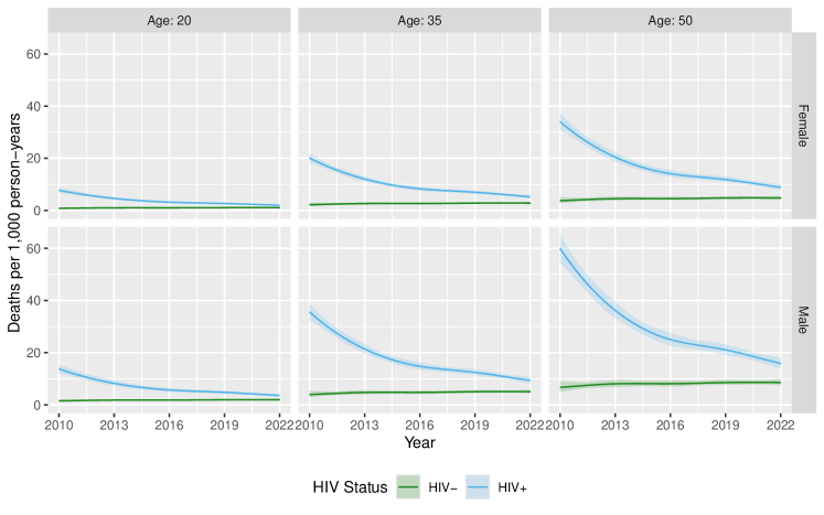
Figure 1: Conditional mortality rates (number of deaths per 1,000 person-years) by calendar time and HIV status, shown for several combinations of age and sex.

Figure 2 shows modeled mortality rates as a function of age for several combinations of calendar year and sex, disaggregated by HIV status, along with pointwise confidence intervals.

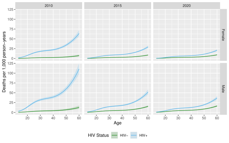
Figure 2: Conditional mortality rates (number of deaths per 1,000 person-years) by age and HIV status, shown for several combinations of calendar time and sex.

Figure 3 plots the discrete hazard of seroconversion (i.e., the probability that an individual will seroconvert in a single year) as a function of age for several combinations of calendar year and sex, along with pointwise confidence intervals. The general decrease in seroconversion rates between 2010 and 2020 is consistent with trends previously reported for similar populations in South Africa (Vandormael et al., 2019, Johnson et al., 2022).

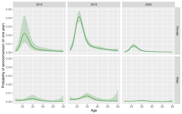
Figure 3: Conditional seroconversion discrete hazards (probability of seroconversion in one year) by age, shown for several combinations of calendar time and sex.

Figure 4 shows the hazard ratio of HIV+ individuals (relative to HIV- individuals) with respect to mortality risk as a function of calendar time, along with pointwise confidence intervals.

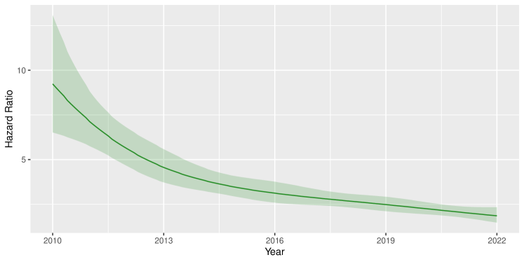
Figure 4: Hazard ratio for mortality, for HIV+ status relative to HIV- status over calendar time.

5 Discussion

In this paper, we described a discrete-time survival model that can be fit via maximum likelihood and used in applications involving an interval-censored covariate representing the occurrence of a secondary event that influences the conditional hazard of the primary event. In the context of the HIV serostatus application, the method proposed in this paper provides a way to fit a survival model using all available data on testing and outcomes. Historically, researchers have removed all data prior to the first HIV test (such that patients enter the risk set at the time of the first test) and/or all data at some point (e.g., two years) after the last HIV negative test. Both methods are ad-hoc and lead to a large proportion of observation time being discarded. The latter is particularly problematic for studies of long-term health outcomes (e.g., chronic disease incidence and mortality), because it leads to the majority of outcome data being discarded for individuals for whom the most recent HIV test is negative.

We considered the case in which there was a single secondary event. This implied that the conditional PMF given in (3) could be computed (for a given individual) as a sum over $k+1$ terms, where $k$ is the number of time points measured for that individual. If there are multiple secondary events, then the set $\mathcal{X}$ in (3) over which the marginalization is done will be of size $(k+1)^{2}$, which may substantially affect computation time. However, computationally feasibility is the only real challenge to generalizing this approach to multiple secondary events. Additionally, if the secondary events are dependent or sequential (e.g., one event cannot occur before the other), the size of $\mathcal{X}$ can be decreased further. One example of such a secondary event is starting antiretroviral therapy, since this cannot happen (for all practical purposes) before a patient seroconverts and tests positive.

It is possible to approach this problem by constructing an EM algorithm, as was done in Goggins et al. (1999) and Ahn et al. (2018). One disadvantage of this approach is that it would require the user to integrate the full likelihood with respect to the density of the secondary event conditional on the primary event (and other covariates); this is possible, but difficult to specify in a principled way since the occurrence of the secondary event is assumed to influence the hazard of the primary event, and not vice versa. A second disadvantage is that EM algorithms are known to often be computationally intense and require many iterations to achieve convergence (Ng et al., 2012).

The findings from the data analysis in section 4 build on evidence from other studies of HIV incidence and risk of mortality among groups defined by HIV serostatus. In a study of the same population-based cohort, Vandormael et al. (2019) estimated incidence using a series of surveys involving HIV testing and observed an overall decrease of 43% between 2012 (0.040 seroconversion events per person-year) and 2017 (0.023 seroconversion events per person-year). Although incidence estimation is not the main goal of the model described in this paper, it is reassuring to see similar trends (see Figure 3), and an analysis allowing for more direct comparisons is a worthwhile future research direction. Reniers et al. (2014) also examined mortality rates by HIV status in a multi-country analysis, dealing with interval-censored serostatus by (1) assuming individuals who had a negative test followed by a positive test seroconvert at the midpoint between the two tests, and (2) censoring HIV- individuals after a certain (age-specific) period of time following their last negative test, and (3) censoring all individuals prior to their first HIV test. In their South Africa site (a different site than the cohort that we analyzed) in 2010, they estimate a mortality rate (per 1,000 person-years) of roughly 70 among HIV+ males, 25 among HIV+ females, 10 among HIV- males, and 5 among HIV- females, yielding sex-specific hazard ratios of roughly 7 and 5 among males and females, respectively. The hazard ratio estimated from our model in 2010 (which we assumed to be the same between males and females) was 9.2 (95%CI: 6.5 – 13.1), and mortality rates were comparable, although a direct comparison is difficult due to differences in the person-time inclusion criteria between the two analyses. Rough alignment of both the seroconversion model and the mortality model with existing estimates is encouraging.

One limitation of the approach taken here is that, in some applications, it will require researchers to “artificially” discretize the data, which involves both a coarsening of the data and the adding of many additional rows to the dataset. As the discretization grid becomes finer (i.e., as the time intervals shrink in length), the loss of information due to coarsening should decrease, eventually to the point of negligibility, but computation time will increase. Thus, there is a trade-off between computation time and precision that will need to be assessed in each application individually; this is a feature common to all discrete survival models. Additionally, putting datasets into a longer format in which individuals contribute multiple rows of person-time often has to be done anyways, as one would do when fitting a Cox model with time-varying covariates. A full discussion of the relative merits of continuous-time versus discrete-time survival models is outside the scope of this work; see, for example, Suresh et al. (2022).

A second limitation of this approach is that it assumes the conditional hazard of the primary event of interest depends only on whether or not the secondary event occurred, rather than the time since its occurrence. In cases in which no individuals have experienced the secondary event at the start of the study, this represents a straightforward extension to the current work, since the “time since secondary event” variable can be computed deterministically for each element of the set $\mathcal{X}$ in (3). However, if for some individuals, the event can occur before the start of the observation window (as is the case in the HIV motivating dataset), this extension becomes more difficult, as one must posit a model for the conditional distribution of the “time since secondary event” variable at the start of the observation window, the parameters of which may be difficult or impossible to fit for a given dataset without making strong assumptions. If this assumption is violated, the hazard ratio for the secondary event will represent a weighted average of the time-specific (time since secondary event) hazard ratios.

A third limitation is that this model assumes a full parametric likelihood for the observed data and the missingness mechanism; if any components of the model are misspecified, estimators may be biased and inference will be invalid; this is a limitation of parametric models in general. In particular, we are assuming that, conditional on covariates, individuals for whom we have no testing data are not systematically different from individuals for whom testing data are available in terms of their risk of seroconversion. This assumption may not be true in practice, and it would be sensible to conduct a sensitivity analysis in which the individuals with no testing data are excluded.

Appendix A References