Graph neural network surrogate for strategic transport planning

Abstract

As the complexities of urban environments continue to grow, the modelling of transportation systems become increasingly challenging. This paper explores the application of advanced Graph Neural Network (GNN) architectures as surrogate models for strategic transport planning. Building upon a prior work that laid the foundation with graph convolution networks (GCN), our study delves into the comparative analysis of established GCN with the more expressive Graph Attention Network (GAT). Additionally, we propose a novel GAT variant (namely GATv3) to address over-smoothing issues in graph-based models. Our investigation also includes the exploration of a hybrid model combining both GCN and GAT architectures, aiming to investigate the performance of the mixture. The three models are applied to various experiments to understand their limits. We analyse hierarchical regression setups, combining classification and regression tasks, and introduce fine-grained classification with a proposal of a method to convert outputs to precise values. Results reveal the superior performance of the new GAT in classification tasks. To the best of the authors’ knowledge, this is the first GAT model in literature to achieve larger depths. Surprisingly, the fine-grained classification task demonstrates the GCN’s unexpected dominance with additional training data. This shows that synthetic data generators can increase the training data, without overfitting issues whilst improving model performance. In conclusion, this research advances GNN based surrogate modelling, providing insights for refining GNN architectures. The findings open avenues for investigating the potential of the newly proposed GAT architecture and the modelling setups for other transportation problems.

1 Introduction

Transportation plays a critical role in today’s society. The modern urban landscape is characterized by ever-increasing mobility demands, necessitating sophisticated and efficient transport systems. Strategic transport planning plays a pivotal role in shaping the future, to meet the needs of growing populations and evolving societal demands. However, the complexity of urban environments, with their intricate networks of roads, public transit systems, and diverse travel patterns, presents a formidable challenge in accurately modelling and simulating transportation systems.

In recent years, the development of surrogate models has emerged as a promising approach to tackle the complexity of strategic transport planning. Surrogate models are easier to apply and have been shown to even surpass the performance of the original models in other fields (e.g., Choi & Kumar, 2024). Furthermore, such models can also be tuned directly using data and auto-calibration procedures are available. User-friendly models like these that can evaluate complex mobility options are being expected much by the city authorities [Narayanan et al., 2023].

For strategic transport planning, a prior study [Narayanan et al., 2024] laid the foundation by investigating the feasibility of constructing a surrogate through the application of Graph Convolution Network (GCN) in both classification and regression setups. This is a primary work to ascertain whether Graph Neural Network (GNN) based surrogates can even replicate the traditional strategic modelling approach (i.e., the four step model), which could pave way to replicate complex approaches like agent-based models in future. While the study demonstrated initial promise, the potential for further refinement and enhancement of surrogate modelling techniques remains untapped.

This paper builds upon the foundation laid in the pioneer work of Narayanan et al. [2024], through the exploration of advanced neural network architectures and different task setups. We delve into the comparative analysis of the established GCN model with the more recent and expressive Graph Attention Network (GAT). Additionally, we introduce a novel variant of GAT tailored to address the prevalent issue of over-smoothing in graph-based models. Furthermore, to push the boundaries of surrogate modelling even further, we investigate the synergistic potential of combining both GCN and GAT architectures. We also explore the realm of hierarchical regression setups, where we explore the integration of classification and regression tasks. This holistic approach seeks to investigate whether there exist benefits in combining both the types of tasks.

To avoid the issues associated with the complexity of regression and hierarchical setups while ensuring the possibility of obtaining precise values, we delve into the realm of fine-grained classification combined with a method to convert its output to precise values. Finally, a synthetic data generator is implemented to study the impact of increasing the training data. Through this research endeavor, we aim to not only expand the horizons of GNN based surrogate modelling in strategic transport planning, but also provide insights and methodologies for enhancing the applicability and usability of such models in urban planning scenarios.

The methodological framework of this study is outlined in Figure 1. Section 2 provides a brief review of the prior work. Section 3 elaborates on the methodology, detailing the datasets and the architectures of GAT and the proposed variant. It also introduces the hybrid model (GCN+GAT). Section 5 presents the experimental results, which consists of (i) comparison between the different GNN models, (ii) hierarchical regression task and (iii) fine grained classification task. Finally, Section 6 offers concluding remarks and outlines avenues for future research.

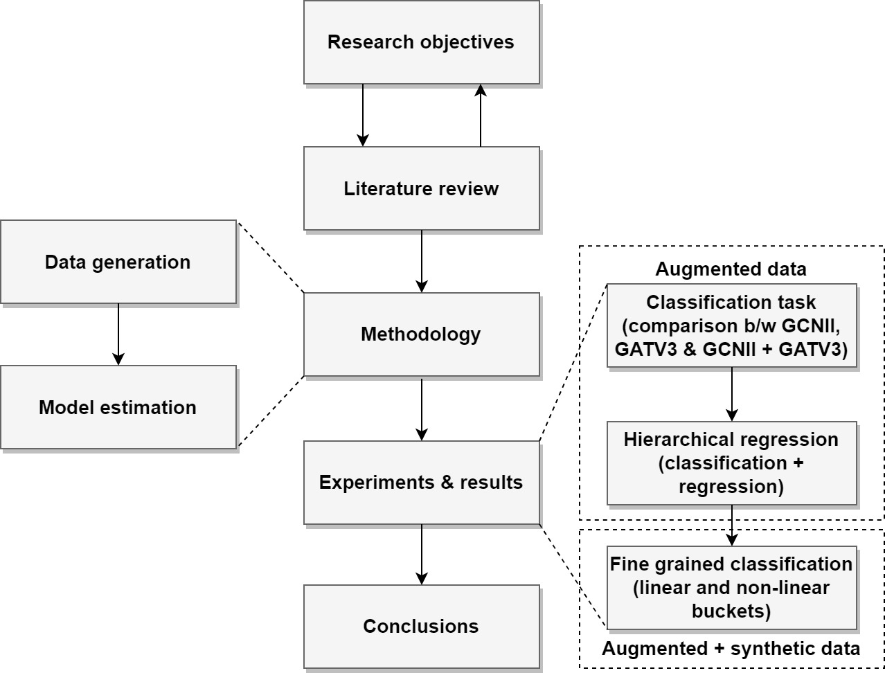
Figure 1: Methodological framework

2 Literature review

This section focuses on the existing literature related to the application of (i) GNNs and (ii) surrogate models for transport planning. The reviewed studies were gathered through the Scopus database using an open source python script from Narayanan & Antoniou [2022].

2.1 GNNs for transport planning

GNNs are slowly gaining significant traction in the domain of transport planning due to their ability to capture intricate spatial dependencies within complex urban networks. For example, GNNs are used to predict the demand for micromobility modes. In this direction, Lin et al. [2018] proposes Graph Convolutional Neural (GCN) Network model to forecast station-level hourly demand for a bike-sharing system in New York City and conclude that such models show promising results. Ding et al. [2022] utilised a GNN model to study the effect of a dockless bike-sharing scheme on the the demand of the London Cycle Hire scheme. For a shared E-scooter system, Song et al. [2023] developed a GNN model to predict the demand in Louisville, USA. Both of these studies also conclude that GNN models make better predictions.

GNNs are also used for studying taxi trips. For example, Wang et al. [2024] developed a spatio-temporal GNN model for taxi route assignment. Tygesen et al. [2023] conduct experiments on NYC Yellow Taxi and provide insights on the kinds of connections GNNs use for spatio-temporal predictions in the transport domain. They also perform tests for short term traffic prediction. Similarly, Cui et al. [2020] incorporate graph wavelet and employ gated recurrent structure for network-wide traffic forecasting. Xu et al. [2023] conclude that graph based models perform better than other machine learning models for network-wide short-term traffic speed prediction and imputation. Graph based neural network models are also used for real-time incident prediction (e.g., Tran et al., 2023) and can be helpful in solving the air transportation nexus among safety, efficiency and resilience [Wandelt et al., 2024].

2.2 Surrogate modelling in the field of transportation

Surrogate modelling is a macro-modeling technique to approximate expensive functions and to replicate input–output relationships. Surrogate models are also called meta- or response surface models and posses beneficial qualities, such as cheaper evaluation costs and sometimes, better accuracy. To approximate complex simulation systems, deep learning based surrogate models are appropriate, as they are suitable to represent non-linear relationships and can handle high dimensional problems well. In the field of traffic forecasting, Vlahogianni [2015] introduces the concept of surrogate modelling and suggests some approaches to specific optimization problems that a transportation researcher may face when dealing with forecasting models. The approaches can be adapted to various transportation problems and the results convey that surrogate models can generate more accurate predictions in significantly reduced times.

Focusing on dynamic user equilibrium, Ge et al. [2020] formulates a dynamic user equilibrium traffic assignment model incorporating surrogate dynamic network loading models. They conclude that the usage of surrogate approaches reduces the computational times by up to 90%, while at the same time, leading to lower errors. Surrogate models are also used to assign Dedicated Bus Lanes (DBLs) across a large-scale road network. The results of numerical studies from Li et al. [2022] show that surrogate based methods for optimal DBL allocation scheme can save a substantial amount of time, especially with limited computational resource, while also leading to around 5% better network performance than the costly simulation approaches.

The concept of GNN based surrogate modelling in the context of transport modelling emerged very recently, with the pioneering work of Narayanan et al. [2024]. They laid a foundational groundwork by investigating the feasibility of developing a GCN based surrogate for strategic transport planning. Their study delve into both classification and regression setups, and based their analysis by generating data from Greater Munich metropolitan region. The experimental results show that GNNs have the potential to act as transport planning surrogates and the deeper models perform better than their shallow counterparts. However, the models suffer performance degradation with an increase in network size.

2.3 Summary and research gaps

In this section, a summary of the reviewed studies and the identified gaps are provided, which act as a motivation for the research objectives of this study. On the one hand, the existing literature on the application of GNNs shows that they have the potential to be utilised for transport modelling. On the other hand, surrogate models are found to be computationally effective and generate more accurate outputs. Therefore, it is advantageous to develop a GNN surrogate for strategic transport planning, the foundation for which has already been laid by Narayanan et al. [2024].

The study of Narayanan et al. [2024] demonstrated the efficacy of GCNs and showcased how GCNs outperformed traditional machine learning models by effectively leveraging the graph structure inherent in transportation networks. Nevertheless, the limitations of GCNs (e.g., the neighbourhood aggregation function used in the GCN puts equal weight on all neighbours, while all neighbours may not be equally relevant) and that of the classification and regression setups necessitate the investigation of the use of advanced GNN architectures and the analysis of novel modelling setups, which will be the focus of this study.

3 Methodological framework

This study builds over the methodological framework established in Narayanan et al. [2024]. Therefore, the procedural sequence is as follows: (i) data generation for the four-step model, (ii) simulation in the four-step model, (iii) data transformation (i.e., direct graph) and the creation of the training data (iv) GNN model training and model evaluation. The regularization methods (i.e., Dropout and GraphNorm), loss functions (cross entropy for the classification tasks and mean squared error for the regression tasks) and evaluation metrics (accuracy and F1-score for the classification tasks and mean absolute error and R²) from there are also utilised in this study. For detailed information of the setup, the reader is referred to the original study.

As an addition to the existing setup, this study develops and investigates another data generation process and further GNN models, which are introduced in the below sections. The implementation of the entire pipeline is performed in Python. The baseline models are estimated using Scikit-Learn [Pedregosa et al., 2011]. GNN models are implemented in PyTorch Geometric [Fey & Lenssen, 2019], which is an extension to the PyTorch library [Paszke et al., 2019]. Due to privacy concerns, the entire code (including the ones for data generation and processing) is provided in a private GitHub repository, which is found at https://github.com/nikita68/4_step_model_surrogate. Access to it is possible upon request. Nevertheless, the processed datasets are separately available at https://github.com/nikita6187/TransportPlanningDataset.

3.1 Synthetic data generation

For data generation, Narayanan et al. [2024] implemented augmented data generation, wherein the network of Munich metropolitan region is used to generate multiple subnetworks for model training. It is often seen that more data significantly helps deep learning models [Wang et al., 2017]. However, the original network data source utilised for the augmented dataset in Narayanan et al. [2024] has only a finite number of possible subnetworks, until the training dataset has a critical overlap with the validation and test datasets. To overcome this issue, while still providing arbitrarily more data, this study implements additional data generation procedure, namely the synthetic data generation.

A synthetic region generation algorithm is implemented, which does not use any original network as a source. This algorithm is motivated based on the works of [Parish & Müller, 2001, Smelik et al., 2014, Cogo et al., 2019]. Assuming that the target amount of nodes ($\mathds{G}_{nodes}$) is provided as input, along with the components for generating zones and zonal information (as identical to that of the augmented data generation procedure), the algorithm performs the following steps:

1. Create the required number of random nodes $\mathds{G}_{nodes}$ within a square region.

2. Calculate the number of zones to be created, i.e., $\mathds{G}_{zones}=\mathds{G}_{nodes}*\mathds{G}_{zones/nodes}$. Select $\mathds{G}_{zones}$ among $\mathds{G}_{nodes}$, which are furthest away from each other to become zonal nodes.

3. Generate zonal information on the previously selected (zonal) nodes.

4. Generate routes between the zones in two steps.

   1. Create $\mathds{G}_{zones}$ number of routes. Each route is created by randomly selecting two zones based on their number of residents and employees. Next, a simple heuristic algorithm starts at a node, examines the closest 7 neighbours, and selects the neighbour which is closest to the target zone as the next step along the route. This is repeated until the route is finished.

   2. Next, if any zone is not yet connected to the network, apply the above routing algorithm to the closest node part of the existing network.

5. Delete the nodes that are not connected and split long segments of the network until target number of nodes is reached.

6. Run the four step model on the data, and save the data and the output of the four step model.

The synthetic dataset is generated with 10000 samples, with a target number of nodes between 15 and 80. Note, the synthetic dataset is used in this paper only as supplementary training data for the augmented dataset with further details being provided in the experiments section (Section 4).

3.2 Graph attention networks

Narayanan et al. [2024] developed a GNN surrogate based on Graph Convolutions Networks (GCN). The neighbourhood aggregation function used in the GCN puts equal weight on all neighbours. However, not all neighbours may be equally relevant. An example would be an incoming road having a high traffic demand, whilst another having zero at a junction. Thus, the information relevant for the outgoing road comes more from the high demand incoming road. Therefore, in this section, the graph attention networks are presented, together with a novel extension to enable them to generalize to deeper networks.

To be able to understand the difference between different neighbours, the concept of attention was introduced to form the Graph Attention Networks (GAT) [Brody et al., 2021]. Attention is determined by calculating a set of weights for each neighbour of a node, with every weight being between 0 and 1, and all the weights summing up to 1. When summing up the transformed feature vectors of a node’s neighbours, the vectors are multiplied by the respective weights. The weights themselves are calculated by applying a one layer MLP, which takes in both the original node’s and its neighbour’s feature vector as input. Please note that the GAT model estimated in this study is GATv2 [Veličković et al., 2018, Brody et al., 2021].

Both GATv1 and GATv2 still suffer from the over-smoothing problem, much like the original GCN. This results in both models performing poorly when trying to stack more than 5 layers. To the best of the authors’ knowledge, there is no solution available to this problem at the time of this study. Inspired by the results of GCNII, a novel extension is proposed to use the same simple residual trick from [Chen et al., 2020]. Thus, the GATv2 formulation becomes as follows:

$$\begin{split}{\mathbold{n}}_{i}^{j}=&\,\sigma\left((1-\alpha)\cdot\left(\sum_{k\in n(i)\cup\{i\}}\alpha_{ik}\cdot{\mathbold{n}}_{k}^{j-1}\times\mathbold{W}^{j}\right)+\alpha\cdot{\mathbold{n}}_{i}^{0}\right),\\[3.44444pt] &\alpha_{ik}=\,\sigma_{softmax}\left(N_{ff}\left(\left[{\mathbold{n}}_{k}^{j-1};{\mathbold{n}}_{i}^{j-1}\right]\right)\right)_{k},\\[3.44444pt] &\text{with }\sum_{k}\alpha_{ik}=1,\text{ and }\alpha_{ik}\in[0,1].\end{split}$$ (1)

where,
$\alpha$ is a fixed hyperparameter
$\alpha_{ik}$ is the attention weight of node $i$ for neighbour $k$, with the attention weights summing up to 1 for all of a given nodes neighbours, and each weight being between 0 and 1
$\sigma$ is the activation function
$\sigma_{softmax}$ is the activation function that forces all outputs to be between 0 and 1, and normalizes all outputs so that they sum to 1 [Nwankpa et al., 2018]
$k$ represents all the direct neighbours of node $i$
$N_{ff}$ is a one layer MLP
${\mathbold{n}}_{i}^{0}$ is from the input layer for node $i$
${\mathbold{n}}_{i}^{j}$ is the feature of node $i$ in GAT layer $j$
$\mathbold{W}^{j}$ is the weight matrix of layer $j$
$[;]$ operator concatenates the input vectors

Even though it is a minor change performed on the GATv2 model, this solves the issue of developing deeper GAT models, as will be shown in later sections. From now, this model is denoted as $GATv3$. Note that, due to the extra computations, the number of GAT layers which can fit onto one GPU is significantly less than those of GCNs.

3.3 Combined GAT and GCN

The GCNII implemented in Narayanan et al. [2024] and the GATv3 introduced in this study solve the over-smooting problem, but do not specifically focus on over-squashing. Over-squashing is the effect where each additional GNN layer increases exponentially the amount of information that needs to contained within the fixed sized feature vector of a node [Alon & Yahav, 2020]. The effect is shown to result in information loss, which is critical for proper modelling. To the best of the authors’ knowledge, there is no known adequate fix to this problem. The over-squashing problem can potentially pose a major problem for transport planning predictions, as information needs to be exchanged between nodes that are large distances away from each other. This is, especially, important for nodes containing zonal information.

To overcome the aformentioned issue, an attempt has been made to combine the GAT and GCN models. The idea is to first have a number of GATv3 layers, using an artificial graph connecting only zone nodes together. Next, the input is fed through a larger number of GCNII layers, which use the entire network graph. Finally, feed forward layers do the last processing of the data and output link level predictions. The intuition behind this model is similar to that of the strategic transport planning. The first GAT layers focus on determining the demand of the individual zones. The following GCN layers then focus on realistically applying the determined demand onto the existing network. The artificial graph used in the GAT layers is a graph where all zonal nodes are connected, whilst all other nodes are disconnected. This ensures a focus on the socio-economic information governing the demand aspect of transport planning. The model type is called the combined GAT and GCN model, and is abbreviated as $GCN+GAT$.

4 Experimental setup

This section will focus on three distinct setups, i.e., (i) a classification setup to compare the different GNNs, (ii) a hierarchical regression setup to investigate the effect of combining the classification and regression setups and (iii) a fine-grained classification setup to exploit the stability of classification, which also includes the implementation of a small transformation procedure to convert the classification results into actual traffic values. Finally, the impact of additional data will be explored using the fine-grained classification setup.

4.1 Comparison of GCNII, GATv2, GATv3 and GCN+GATv3

The first experiment is focused on comparing the different GNNs. As Narayanan et al. [2024] concluded that the classification problem (or more formally cross entropy) is more stable than the regression loss (i.e., MSE) with respect to the hyperparameters, this comparison will be based on the classification task. The real valued traffic data is inserted into a bucket, with the bucket index then being the target, which is also inspired in part by the levels found in congestion warning systems [Gerstenberger et al., 2018]. The buckets used are $[0\,veh/h,10\,veh/h)$, $[10\,veh/h,500\,veh/h)$, $[500\,veh/h,\infty\,veh/h)$. These three buckets ensure that each bucket has enough samples, with a 62%, 21% and 17% distribution respectively on the validation dataset. The buckets correspond to no transport usage, low transport usage and medium/high transport usage.

The augmented dataset is used. All the models in this experiment are evaluated using the average F1 score. For the GCNII, a grid search is performed over the number of GCNII layers $\in$ (5, 10, 50, 70), the size of each layer $\in$ (64, 256, 512), $\alpha$ $\in$ (0.1, 0.4) and $\theta$ $\in$ (0.5, 1.5). The best performing model on the validation dataset is based on 70 layers, each layer containing 512 hidden units, $\alpha$ = 0.1 and $\theta$ = 1.5. If not stated otherwise, the same parameters are used for all future GCNII experiments. This experiment further investigates whether the more expressive GAT models improve the predictions. In the preliminary analysis, it was observed that the GATv2 model had convergence problems when attempting to stack more than 5 layers, which is also supported by the observations in the literature [Chen et al., 2020]. Due to the average graph diameter of the dataset being 36, it is mathematically impossible for a shallow GATv2 model to correctly capture the underlying travel patterns. Thus, a GATv3 grid search is performed, with either 20 hidden layers and 512 hidden units or 40 hidden layers with 256 hidden units. Based on the validation dataset, the best configuration is 20 hidden layers with 512 hidden units. Finally, to explore whether the over-squashing and over-smoothing problems can be overcome, the combined GCNII and GATv3 model is investigated. Here, two configurations are explored, either 5 or 10 layers of GATv3 (using the zone connected graph), whilst the following 60 layers are GCNII layers using the full network graph. The best model is found to contain 10 GATv3 layers.

4.2 Hierarchical regression

Classification has less data parameters to tune, thus making it often more stable than regression, but does not produce exact values. To combine both the approaches, the hierarchical regression setup is investigated, which to the best of the authors’ knowledge, does not exist in literature. The core idea is to first predict the bucket in which the transport usage should be. In the next step, given the bucket prediction, a value is outputted between -1 and 1, so as to be able to predict exact values for any bucket by applying normalization. Using the bucket and the regression prediction, it is then possible to determine the exact value being predicted. The core idea of the approach is to combine the stability of classification with the precision of regression.

The input data setup is identical to the previous experiment, i.e., using the augmented dataset and direct graph conversion. The output data is transformed to have two targets: the bucket class and the scaled value within that bucket. The configuration of the output data is thus dependent on the buckets selected. A number of bucket configurations are explored, using the same manual search strategy as employed in the previous regression experiments. The tested bucket groups are the following:

• Bucket T1 - Buckets [0, 10), [10, 500), $>$500 veh/h - investigated due to their success in the previous experiments

• Bucket T2 - Buckets [0, 100), [100, 500), $>$500 veh/h - inspired by the first bucket configuration, but to have more equal sized buckets, without skewing the sample distribution too much

• Bucket T3 - Buckets [0, 10), [10, 100), [100, 200), [200, 500), [500, 1000), [1000, 2000), $>$2000 veh/h - to exploit the high number of data points available in the first few buckets

• Bucket T4 - Buckets going in steps of 100 veh/h from 0 to 4500 - covers all the data points with equidistant buckets

As base GNN model, the GCNII is taken with 70 GCNII layers, each with 512 hidden units, $\alpha=0.1$ and $\theta=1.5$. All the models are trained for 300 epochs, taking around 8-12 hours per training run. To implement the hierarchical regression, the classification is performed by two feed forward layers followed by a softmax activation function. The argmax is taken for this output, and then an embedding vector of size 32 is retrieved for this class, inspired by a similar mechanism in natural language processing [Bahar et al., 2020]. The embedding vector is then concatenated to the output of the GCNII layers, and is used by two feed forward layers to produce the output of the link using the tanh activation function, for determining the exact value. A formal definition is as follows:

$$g(x)_{i}= \,0.5\cdot\left(1+g^{regr}\left(\left[{\mathbold{n}}_{i}^{K};N_{embedding}\left(g^{class}({\mathbold{n}}_{i}^{K})\right)\right]\right)\right)\,\,\cdot$$ (2)

$$\cdot\,\,\left(b_{g^{class}({\mathbold{n}}_{i}^{K}),2}-b_{g^{class}({\mathbold{n}}_{i}^{K}),1}\right)+b_{g^{class}({\mathbold{n}}_{i}^{K}),1}$$ (3)

$$g^{regr}(x)= \,\sigma_{tanh}\left(N_{ff}\left(\sigma_{relu}\left(N_{ff}\left(x\right)\right)\right)\right)$$ (4)

$$g^{class}(x)= \,\operatorname*{arg\,max}_{k}\left[\sigma_{softmax}\left(N_{ff}\left(\sigma_{relu}\left(N_{ff}\left(x\right)\right)\right)\right)_{k}\right]$$ (5)

where,
$g(x)_{i}$ is the final output of the model for link i
$g^{regr}(x)_{i}$ is the output of the regression model for link i
$g^{class}(x)_{i}$ is the output of the classification model for link i $N_{ff}$ is a single feed forward layer
${\mathbold{n}}_{i}^{K}$ is the output of the last layer of the GCNs
$[;]$ is the concatenating operator
$b_{g^{class}({\mathbold{n}}_{i}^{K}),2}$ is the upper bucket value predicted by the classification model
$b_{g^{class}({\mathbold{n}}_{i}^{L}),1}$ is the lower value
$N_{embedding}$ function is a differentiable operator that takes a transport usage bucket ID as input and retrieves a differentiable vector out of memory

The aim of the $N_{embedding}$ is to make the neural network automatically learn to represent each bucket with its own custom vector, without having to explicitly define this vector. An illustration is provided in Figure 2. Training for the classification is done using cross entropy, whilst the regression component is trained using MSE. The losses are added together to form the final loss. Different weightings of the loss functions did not show any difference in performance. To stabilize the training, true labels are used as input to the embedding step, but only during the training of the model. GraphNorm was attempted to be used, but resulted in no convergence for the models. Additionally, residual final layers could not be employed as the use of them lead to GPU memory issues.

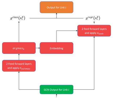
Figure 2: Illustration of the hierarchical regression model.

4.3 Fine grained classification

To further exploit the stability of classification, this experiment is conducted to explore fine grained classification. Furthermore, a method is proposed to convert the classification results into real values. Comparing the F1 score does not make sense when using different buckets, as the the comparison becomes skewed toward the model configurations with fewer buckets. Thus, it makes more sense to use the following metrics: $R^{2}_{\,\geq 10}$ and $MAE_{\,\geq 10}$. However, in classification, only the probabilities are provided as outputs of the model. To convert the probabilities of buckets into a real value, a small transformation procedure is applied using the expectation operator from statistics. Initially, a uniform distribution across each bucket is assumed and the expectation is taken, resulting in the mean value of the bucket. Then, the expectation over all buckets is applied, using the output of the model as the discrete probability distribution. The result is that the model outputs real values in veh/h. Formally,

$$g(x)^{\prime}_{i}=\mathds{E}_{g(x)_{i}}\left[\mathds{E}_{uniform}\left[b_{k}\right]\right]=\sum_{k}g(x)_{i}^{k}\cdot\frac{(b_{k,1}+b_{k,2})}{2}.$$ (6)

where,
$g(x)^{\prime}_{i}$ is the resulting output of the model for the current link $i$
$\mathds{E}_{g(x)_{i}}$ is the expectation using the probabilities provided by the GNN model
$\mathds{E}_{uniform}$ is the expectation over the bucket $k$, assuming a uniform distribution
$g(x)_{i}^{k}$ is the probability from the GNN model for the current link $i$ for bucket k
$b_{k,1}$ is the lower bound of the bucket whilst $b_{k,2}$ is the upper bound

4.3.1 Optimal Bucket Strategy

At first, an optimal bucket strategy needs to be found. A grid search is performed together with a detailed analysis of the best models. The input data is identical to the previous experiments, and the target data is always the bucket index for the classification setup. Two bucketing strategies are conducted: equidistant and non-linear bucketing. For equidistant buckets, the following configurations are explored, as they require little reconfiguration:

• Buckets-e23 - 23 buckets in step size of 200 veh/h

• Buckets-e45 - 45 buckets in step size of 100 veh/h

• Buckets-e90 - 90 buckets in step size of 50 veh/h

• Buckets-e180 - 180 buckets in step size of 25 veh/h

• Buckets-e450 - 450 buckets in step size of 10 veh/h

When looking at the equidistant buckets, it is seen that many of the higher value buckets have no or few training samples, whilst lower values have many thousands of samples. The difference in sample sizes can greatly impact the performance of GNNs, and especially restrict their generalization behaviour. To compensate for this effect, non-linear bucket sizes are also explored, to ensure that all buckets have at least a few training samples. The following configurations are examined:

• Buckets-nl38 - Steps of 25 from 0 veh/h to 250 veh/h, steps of 50 from 250 veh/h to 1000 veh/h, steps of 100 from 1000 veh/h to 1500 veh/h, steps of 500 from 1500 veh/h

• Buckets-nl54 - Steps of 25 from 0 veh/h to 500 veh/h, steps of 50 from 500 veh/h to 1500 veh/h, steps of 100 from 1500 veh/h to 2000 veh/h, steps of 500 from 2000 veh/h

Further configurations are not explored as the results implied that there is no significant further improvement.

4.3.2 Use of additional synthetic data

Synthetic data to increase the training dataset has been shown in existing literature to improve deep learning models [Nikolenko, 2021]. The synthetic dataset is used only to expand the training data, with the validation and test datasets being kept the same as in the previous experiments to ensure proper comparisons. The new training dataset size is more than 2.5 times larger than the original dataset. The two previously best performing bucket configurations (nl54 and e90), as will be observed in Section 5, are then trained from scratch using the additional synthetic training data. Each training run of a model takes around 12-15 hours.

The final experiments examine how the GATv3 and GCN+GAT models perform using the training data supplemented by the synthetic samples. The data setup is identical to the previous experiment, but only using the Buckets-nl54 configuration. The GCNII is used with 70 layers, 512 hidden units, $\alpha=0.1$, $\theta=1.5$, 3 residual feed forward layers, GraphNorm after each convolution operation and a dropout of 25%. The GATv3 model contains 20 layers each with 512 hidden units, based on 2 attention heads performing the averaging merging strategy, 3 residual feed forward layer, GraphNorm and dropout with 25%. Finally, the GCN+GAT model is configured with 10 zonal GATv3 layers, each with 128 hidden units, 2 attention heads being averaged together. Following that, 60 GCNII layers are used, each with 512 hidden units, $\alpha=0.1$, $\theta=1.5$ and 3 residual feed forward layers. GraphNorm and dropout of 25% is used for each convolution layer. Note, each training run takes around 40 hours.

5 Experimental results

The experiments described in the previous section are performed sequentially and the respective results are summarised in this section.

5.1 Evaluation of different GNN architectures (GCNII, GATv3, GCN+GATv3) and hierarchical regression

Different GNN models are compared to find the optimal model setup. The F1 score of all the models can be found in Table 1. It is observed that the GCNII model performs significantly better than all baselines. Note that the accuracy of the model is at 85%, and most errors are observed in classifying the [10 veh/h, 500 veh/h) bin. For the bin of [0 veh/h, 10 veh/h), an accuracy of 95% is achieved. On a different note, the configuration containing both the largest number of layers and largest layer size in the GCNII performs best. The best performing model is the GATv3, followed closely by the GCN+GAT model, and then the GCNII model. All three GNNs perform similarly to each other, and significantly better than the baselines.

Table 1: F1 score corresponding to the test dataset, for the classification task comparing the different GNN models

Model	$F1$ Score
Majority Classifier	0.25
Random Forest	0.54
MLP	0.53
GCNII	0.85
GATv3	0.87
GCN + GAT	0.86

The convergence of all GNN models based on the direct graph is observed to be stable and level out at around 300 epochs. If not otherwise stated, all the presented GNN models in this study have similar convergence behaviour on the training and validation data. It can be concluded that a larger number of layers and thus more trainable parameters are helpful. Additionally, it is observed that all models perform similarly between their test and validation scores, verifying that the generalization of the models is highly probable.

With regards to the model performance, the three GNN models perform well and have only slight variations. First, this implies that deep GNNs are a suitable candidate to further explore for a surrogate model for the four step model. Secondly, it implies that the exact model does not make a major difference. For future experiments, a GCNII can be used for initial experiments, and other GNN models can be tested, once a potential stable problem setup is found. Looking at the GCN+GAT model, it has similar performance to the other models. A hypothesis on this is that either it does not solve the over-squashing problem, or the issue does not exist for this initial task. Further research into this should be examined in future experiments.

Looking at the hierarchical regression, the best model using “Bucket 3” option reaches only 175.8 $MAE_{\,\geq 10}$, significantly worse than the best regression model from Narayanan et al. [2024]. Even though the hierarchical regression models perform better than the baselines, they do not come close to the best model from the classical regression experiments. The subpar performance found in hierarchical regression may be due to the fact that the task is too complex as a problem for the model experimented here. Deeper models with more parameters could potentially be a solution, but there needs to be further research on this topic.

5.2 Evaluation of fine grained classification

In this section, the results of the classification performed on fine grained buckets are presented. By applying the double expectation operator, it is possible to convert probabilities to real values, with all details about the setup found in Section 4.3. With regards to the optimal bucket strategy, the resulting evaluation metrics of the relevant experiments are shown in Table 2. It can be seen that all reach good results, when compared to the baselines. However, only GCNII - Buckets-e90 slightly surpasses the $MAE_{\,\geq 10}$ score of the best regression model. Between the best models of the linear and non-linear bucketing, the latter does not surpass the former.

The two best performing bucket configurations, nl54 and e90, are then trained from scratch using additional synthetic training data. Both the models with the extra data perform significantly better than the baselines, as can be seen in Table 2, and have an 16% better performance than the models without the extra data. However, the best non-linear bucketing model has a slightly better performance than the best linear bucketing model, which is in contrast to the ones without the extra data. Looking more closely at the differences between the models “GCNII - Buckets-e90 - extra data” and “GCNII - Buckets-nl54 - extra data”, it is found that the former predicts high values poorly. As seen in Figure 3, all true values above around 2500 veh/h get assigned values around 2600 veh/h. On the other hand, the model with non-linear 54 buckets continues to predict proportionally high values, as shown in Figure 4. The effect comes probably from the high number of classes having few data points for training in the case of equidistant bucketing.

Table 2: Results of fine grained classification on validation dataset

Model	Validation $R^{2}_{\,\geq 10}$	Validation $MAE_{\,\geq 10}$
Mean Regressor	0.00	394.8
Random Forest	0.00	373.1
MLP	0.00	371.6
GCNII - Regression Best	0.84	131.1
GCNII - Buckets-e23	0.79	145.4
GCNII - Buckets-e45	0.78	140.1
GCNII - Buckets-e90	0.81	129.6
GCNII - Buckets-e180	0.78	139.5
GCNII - Buckets-e450	0.78	137.8
GCNII - Buckets-nl38	0.79	136.1
GCNII - Buckets-nl54	0.79	133.0
GCNII - Buckets-e90 - extra data	0.85	114.8
GCNII - Buckets-nl54 - extra data	0.86	111.4

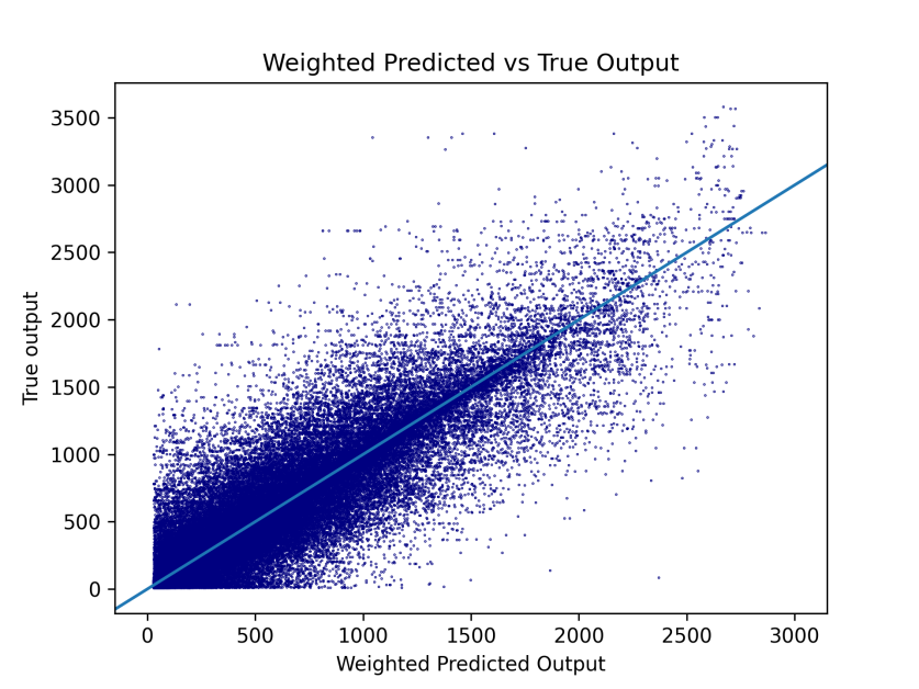
Figure 3: Predicted output vs true output for the GCNII - Buckets-e90 - extra data model on the test dataset. Each point is a prediction for a single link, with both values being in veh/h. An optimal prediction would be along the light blue line. Notice that for true values above 2500, the model constantly predicts around 2600.

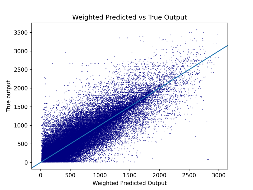
Figure 4: Predicted output vs true output corresponding to the test dataset for the GCNII - Buckets-nl54 - extra data model. Each point is a prediction for a single link, with both values being in veh/h. An optimal predicted would be along the light blue line. Observe that for true values over 2500, the model still predicts proportionally higher output values.

Compared to the regression setting, the fine grained classification returned more consistent results, probably as fewer steps are required. Such behaviour is especially desirable as it requires less configuration searching and reduces the overall model development time. Furthermore, extra synthetic data has shown to make a significant improvement in the performance of the models. To validate the result with more GNNs, GATv3 and GCN+GAT models are trained. The evaluation metrics of the experiment runs can be found in Table 3. The best performing model is the GCNII with extra data, closely followed by the GCN+GAT model. But with GATv3, the performance is comparatively poor. Narayanan et al. [2024] observed the existence of positive correlation between the graph size and the errors in the regression problem, meaning that the GNNs are not able to generalize well to larger networks. The same pattern continue to exist even in the fine grained classification problem, as depicted in Figure 5. On a different note, the improvements observed by increasing the training data is consistent with different GNN models. This implies that more training data is required for better predictions, as is the usual case for the deeper models.

Table 3: Evaluation metrics corresponding to the test dataset for fine grained classification with additional synthetic training data. GATv3 is in parentheses as it experienced overfitting.

Model	Test Set
	$R^{2}_{\,\geq 10}$	$MAE_{\,\geq 10}$
Mean Regressor	0.00	402.6
Random Forest	0.00	383.9
MLP	0.00	382.8
GCNII - Regression Best	0.84	135.4
GCNII - Buckets-nl54	0.79	136.4
GCNII - Buckets-nl54 - extra data	0.85	118.5
GATv3 - Buckets-nl54 - extra data	(0.78)	(144.9)
GCN+GAT - Buckets-nl54 - extra data	0.84	120.0

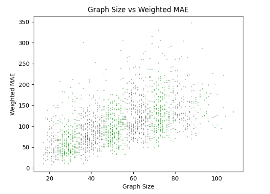
Figure 5: $MAE_{\,\geq 10}$ with respect to graph size, i.e. number of nodes for the trained GCN+GAT model on the test dataset. Each point is the average absolute error of a single graph, with the errors coming from incorrect link transport usage prediction. Highly similar plots are observed for all GNNs.

6 Conclusions

In this study, we embarked on an exploration of surrogate modelling for strategic transport planning, leveraging advanced Graph Neural Network (GNN) architectures. Specifically, we compared the established Graph Convolution Network (GCN) with the more recent and expressive Graph Attention Network (GAT). Additionally, we introduce a novel variant of GAT (namely GATv3) tailored to address the issue of over-smoothing present in graph-based models. Furthermore, we investigate (i) the synergistic potential of combining both GCN and GAT architectures, (ii) the realm of hierarchical regression setups integrating classification and regression tasks and (iii) the realm of fine-grained classification combined with a method to convert its output to precise values, to avoid the issues associated with the complexity of regression and hierarchical setups. Finally, a synthetic data generator is implemented to study the impact of increasing the training data.

Our findings shed light on the performance of various model architectures across distinct tasks, providing valuable insights for future research and application in this domain. Our results underscore the effectiveness of the newly proposed Graph Attention Network (GATv3) in the classification task. Thus, it is possible to develop deep GATs using the GATv3 formulation, which is relevant for problems wherein the feature sharing between distant nodes is important. Furthermore, the superior performance of the new GAT, when compared to existing GATs and the GCN models, highlights its potential as a formidable tool for capturing more intricate patterns within transportation networks. This signifies a significant step forward in refining surrogate models for strategic transport planning.

The combined GAT and GCN model, while exhibiting a marginal improvement over the standalone GCN model, was unable to surpass the performance of the new GAT. This observation suggests that while hybrid architectures hold promise, there is a need for further investigation to increase their synergistic potential. Our exploration into hierarchical regression, which aimed to combine categorical and continuous aspects of transportation dynamics, yielded suboptimal results. This indicates that deeper analysis are warranted to understand the challenges and potential solutions in this specific modelling context. Surprisingly, in the fine-grained classification task with the provision of additional training data (produced through the propsed synthetic data generator), the Graph Convolution Network (GCN) emerged as the top performer. This contrasts with the performance of the new GAT and the combined GAT+GCN models, which, while competitive, fell slightly short. This outcome prompts consideration of potential factors, such as the problem type and the impact of expanded dataset.

To sum up, the answer to whether fine-grained classification can perform well is yes. Additionally, it is observed to be more stable with respect to the model hyperparameters than regression. With an extended training dataset, further performance improvements are reached. Therefore, exploring strategies to augment the dataset could lead to further advancements. Nevertheless, a detailed analysis shows that the positive correlation between network size and error continues to be an issue, which requires further exploration in future. In conclusion, this research represents a significant stride towards refining GNN based surrogate models for strategic transport planning. The insights gleaned from this study pave the way for several promising avenues of future research. The demonstrated superiority of the new GAT in the classification task and the unexpected dominance of GCN in fine-grained classification underscore the need for continued exploration and refinement of GNN architectures in this context. Furthermore, the novel GAT architecture and the modelling setups (such as the hierarchical regression and the fine-grained classification with the possibility of obtaining the exact values) proposed in this study could be explored for other transportation problems. We anticipate that this work will serve as a valuable foundation for future endeavors in enhancing the accuracy and applicability of GNN-based surrogate models in complex urban planning scenarios.

Declaration of interest: None

References

- Alon & Yahav [2020] Alon, U., & Yahav, E. (2020). On the bottleneck of graph neural networks and its practical implications. In International Conference on Learning Representations.
- Bahar et al. [2020] Bahar, P., Makarov, N., & Ney, H. (2020). Investigation of transformer-based latent attention models for neural machine translation. In Proceedings of the 14th Conference of the Association for Machine Translation in the Americas (AMTA 2020) (pp. 7–20).
- Brody et al. [2021] Brody, S., Alon, U., & Yahav, E. (2021). How attentive are graph attention networks? arXiv preprint arXiv:2105.14491, .
- Chen et al. [2020] Chen, M., Wei, Z., Huang, Z., Ding, B., & Li, Y. (2020). Simple and deep graph convolutional networks. In International Conference on Machine Learning (pp. 1725–1735). PMLR.
- Choi & Kumar [2024] Choi, Y., & Kumar, K. (2024). Graph neural network-based surrogate model for granular flows. Computers and Geotechnics, 166, 106015. URL: http://dx.doi.org/10.1016/j.compgeo.2023.106015. doi:10.1016/j.compgeo.2023.106015.
- Cogo et al. [2019] Cogo, E., Prazina, I., Hodzic, K., Haseljic, H., & Rizvic, S. (2019). Survey of integrability of procedural modeling techniques for generating a complete city. In 2019 XXVII International Conference on Information, Communication and Automation Technologies (ICAT). IEEE. URL: https://doi.org/10.1109/icat47117.2019.8939012. doi:10.1109/icat47117.2019.8939012.
- Cui et al. [2020] Cui, Z., Ke, R., Pu, Z., Ma, X., & Wang, Y. (2020). Learning traffic as a graph: A gated graph wavelet recurrent neural network for network-scale traffic prediction. Transportation Research Part C: Emerging Technologies, 115, 102620. URL: http://dx.doi.org/10.1016/j.trc.2020.102620. doi:10.1016/j.trc.2020.102620.
- Ding et al. [2022] Ding, H., Lu, Y., Sze, N., & Li, H. (2022). Effect of dockless bike-sharing scheme on the demand for london cycle hire at the disaggregate level using a deep learning approach. Transportation Research Part A: Policy and Practice, 166, 150–163. URL: http://dx.doi.org/10.1016/j.tra.2022.10.013. doi:10.1016/j.tra.2022.10.013.
- Fey & Lenssen [2019] Fey, M., & Lenssen, J. E. (2019). Fast graph representation learning with PyTorch Geometric. In ICLR Workshop on Representation Learning on Graphs and Manifolds.
- Ge et al. [2020] Ge, Q., Fukuda, D., Han, K., & Song, W. (2020). Reservoir-based surrogate modeling of dynamic user equilibrium. Transportation Research Part C: Emerging Technologies, 113, 350–369. URL: http://dx.doi.org/10.1016/j.trc.2019.10.010. doi:10.1016/j.trc.2019.10.010.
- Gerstenberger et al. [2018] Gerstenberger, M., Hösch, M., & Listl, G. (2018). Überarbeitung und Aktualisierung des Merkblattes für die Ausstattung von Verkehrsrechner- und Unterzentralen (MARZ 1999). Technical Report Bundesanstalt für Straßenwesen (BASt).
- Li et al. [2022] Li, Z., Tian, Y., Sun, J., Lu, X., & Kan, Y. (2022). Simulation-based optimization of large-scale dedicated bus lanes allocation: Using efficient machine learning models as surrogates. Transportation Research Part C: Emerging Technologies, 143, 103827. URL: http://dx.doi.org/10.1016/j.trc.2022.103827. doi:10.1016/j.trc.2022.103827.
- Lin et al. [2018] Lin, L., He, Z., & Peeta, S. (2018). Predicting station-level hourly demand in a large-scale bike-sharing network: A graph convolutional neural network approach. Transportation Research Part C: Emerging Technologies, 97, 258–276. URL: http://dx.doi.org/10.1016/j.trc.2018.10.011. doi:10.1016/j.trc.2018.10.011.
- Narayanan & Antoniou [2022] Narayanan, S., & Antoniou, C. (2022). Electric cargo cycles - A comprehensive review. Transport Policy, 116, 278–303. doi:10.1016/j.tranpol.2021.12.011.
- Narayanan et al. [2024] Narayanan, S., Makarov, N., & Antoniou, C. (2024). Graph neural networks as strategic transport modelling alternative - A proof of concept for a surrogate. IET Intelligent Transport Systems, Under review.
- Narayanan et al. [2023] Narayanan, S., Salanova Grau, J. M., Frederix, R., Tympakianaki, A., Masegosa, A. D., & Antoniou, C. (2023). Modeling of shared mobility services - an approach in between aggregate four-step and disaggregate agent-based approaches for strategic transport planning. Journal of Intelligent Transportation Systems, (pp. 1–18). doi:10.1080/15472450.2023.2246374.
- Nikolenko [2021] Nikolenko, S. I. (2021). Synthetic Data for Deep Learning. Springer International Publishing. URL: http://dx.doi.org/10.1007/978-3-030-75178-4. doi:10.1007/978-3-030-75178-4.
- Nwankpa et al. [2018] Nwankpa, C., Ijomah, W., Gachagan, A., & Marshall, S. (2018). Activation functions: Comparison of trends in practice and research for deep learning. arXiv preprint arXiv:1811.03378, .
- Parish & Müller [2001] Parish, Y. I. H., & Müller, P. (2001). Procedural modeling of cities. In Proceedings of the 28th annual conference on Computer graphics and interactive techniques - SIGGRAPH '01. ACM Press. URL: https://doi.org/10.1145/383259.383292. doi:10.1145/383259.383292.
- Paszke et al. [2019] Paszke, A., Gross, S., Massa, F., Lerer, A., Bradbury, J., Chanan, G., Killeen, T., Lin, Z., Gimelshein, N., Antiga, L., Desmaison, A., Kopf, A., Yang, E., DeVito, Z., Raison, M., Tejani, A., Chilamkurthy, S., Steiner, B., Fang, L., Bai, J., & Chintala, S. (2019). Pytorch: An imperative style, high-performance deep learning library. In H. Wallach, H. Larochelle, A. Beygelzimer, F. d'Alché-Buc, E. Fox, & R. Garnett (Eds.), Advances in Neural Information Processing Systems 32 (pp. 8024–8035). Curran Associates, Inc. URL: http://papers.neurips.cc/paper/9015-pytorch-an-imperative-style-high-performance-deep-learning-library.pdf.
- Pedregosa et al. [2011] Pedregosa, F., Varoquaux, G., Gramfort, A., Michel, V., Thirion, B., Grisel, O., Blondel, M., Prettenhofer, P., Weiss, R., Dubourg, V., Vanderplas, J., Passos, A., Cournapeau, D., Brucher, M., Perrot, M., & Duchesnay, E. (2011). Scikit-learn: Machine learning in Python. Journal of Machine Learning Research, 12, 2825–2830.
- Smelik et al. [2014] Smelik, R. M., Tutenel, T., Bidarra, R., & Benes, B. (2014). A survey on procedural modelling for virtual worlds. Computer Graphics Forum, 33, 31–50. URL: https://doi.org/10.1111/cgf.12276. doi:10.1111/cgf.12276.
- Song et al. [2023] Song, J.-C., Hsieh, I.-Y. L., & Chen, C.-S. (2023). Sparse trip demand prediction for shared e-scooter using spatio-temporal graph neural networks. Transportation Research Part D: Transport and Environment, 125, 103962. URL: http://dx.doi.org/10.1016/j.trd.2023.103962. doi:10.1016/j.trd.2023.103962.
- Tran et al. [2023] Tran, T., He, D., Kim, J., & Hickman, M. (2023). Msgnn: A multi-structured graph neural network model for real-time incident prediction in large traffic networks. Transportation Research Part C: Emerging Technologies, 156, 104354. URL: http://dx.doi.org/10.1016/j.trc.2023.104354. doi:10.1016/j.trc.2023.104354.
- Tygesen et al. [2023] Tygesen, M. N., Pereira, F. C., & Rodrigues, F. (2023). Unboxing the graph: Towards interpretable graph neural networks for transport prediction through neural relational inference. Transportation Research Part C: Emerging Technologies, 146, 103946. URL: http://dx.doi.org/10.1016/j.trc.2022.103946. doi:10.1016/j.trc.2022.103946.
- Veličković et al. [2018] Veličković, P., Cucurull, G., Casanova, A., Romero, A., Liò, P., & Bengio, Y. (2018). Graph attention networks. In International Conference on Learning Representations.
- Vlahogianni [2015] Vlahogianni, E. I. (2015). Optimization of traffic forecasting: Intelligent surrogate modeling. Transportation Research Part C: Emerging Technologies, 55, 14–23. URL: http://dx.doi.org/10.1016/j.trc.2015.03.016. doi:10.1016/j.trc.2015.03.016.
- Wandelt et al. [2024] Wandelt, S., Sun, X., & Zhang, J. (2024). Graphcast for solving the air transportation nexus among safety, efficiency, and resilience. Communications in Transportation Research, 4, 100120. URL: http://dx.doi.org/10.1016/j.commtr.2024.100120. doi:10.1016/j.commtr.2024.100120.
- Wang et al. [2024] Wang, F., Bi, J., Xie, D., & Zhao, X. (2024). Quick taxi route assignment via real-time intersection state prediction with a spatial-temporal graph neural network. Transportation Research Part C: Emerging Technologies, 158, 104414. URL: http://dx.doi.org/10.1016/j.trc.2023.104414. doi:10.1016/j.trc.2023.104414.
- Wang et al. [2017] Wang, J., Perez, L. et al. (2017). The effectiveness of data augmentation in image classification using deep learning. Convolutional Neural Networks Vis. Recognit, 11, 1–8.
- Xu et al. [2023] Xu, M., Di, Y., Ding, H., Zhu, Z., Chen, X., & Yang, H. (2023). Agnp: Network-wide short-term probabilistic traffic speed prediction and imputation. Communications in Transportation Research, 3, 100099. URL: http://dx.doi.org/10.1016/j.commtr.2023.100099. doi:10.1016/j.commtr.2023.100099.