Average Degree of Graphs Derived From Aperiodic Tilings

Abstract.

We consider graphs derived from aperiodically ordered tilings of the plane, by treating each corner of each tile as a vertex and each side of each tile as an edge. We calculate the average degree of these graphs. For the Ammann A2 tiling, we present a closed-form formula for the average degree. For the Kite and Dart Penrose tiling, the Rhomb Penrose Tiling, and the Ammann-Beenker tiling we present numerical calculations for the average degree.

Keywords: Aperiodic tilings, Average degree,

1. Introduction

A plane tiling is a countable family of closed sets which cover the plane without gaps or overlaps.[GS87]  

Consider the tiling in Figure 1. This is a typical monohedral tiling. “Monohedral" means all the tiles in it have same size and shape.

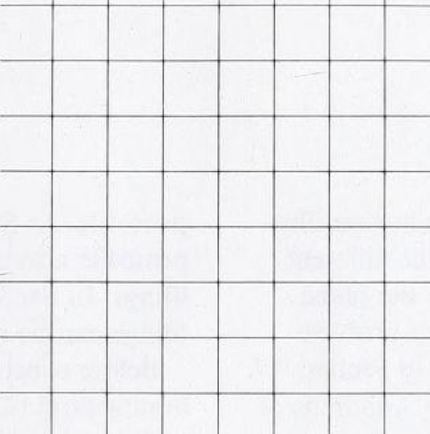
Figure 1. Tiling with Squares

We say that this square tiling is periodic, since it is invariant under a nontrivial translation: translating every tile up, down, left or right by a distance equal to the square length will result in the exact same tiling. Roger Penrose first discovered a pair of tiles that could cover the plane in a non-periodic way, which we generally called aperiodic tilings. The aperiodic tilings Penrose discovered are created through a recursive substitution rule. One of the Penrose tilings uses a pair of tiles shaped like a kite and a dart, while another Penrose tilings uses two tiles, both shaped like rhombuses [Pen74]. These designs are based on the regular pentagon [Pen79].  

In 1982, F.P.M. Beenker, discovered a new tiling using a rhombus tile and a square tile. This tiling is known as the Ammann-Beenker tiling, whilch is also aperiodic. The Ammann-Beenker Tiling is also called as Ammann A1[BM82].

In 1992, Robert Ammann, Branko Grünbaum and Geoffrey C Shephard identified a total of four aperiodic tilings: A2, A3, A4, A5. In this report, we discuss only the Ammann A2 set, which consists of two hexagonal tiles, known as an A-supertile and an enlarged A-tile [AGS92].  

These aperiodic substitution tilings are important as two-dimensional models of quasicrystals. See [BG13] and [BG17] for a more detailed exposition of these tilings from this mathematical crystallography perspective. Also, see the Tilings Encyclopedia website [FGH24] for a compilation of different types of aperiodic tilings.

In this paper we will consider graphs corresponding to these tilings. That is, given a tiling of a plane or a subset of a plane, the graph corresponding to it arises when we treat each corner of every tile as a vertex of the graph, and each side of the tile as an edge.

These graphs corresponding to the Penrose tilings and other aperiodic subtitution tilings have proved useful in physics and engineering: see [FSP20], [LBS⁺22], [MDH⁺22], [DBS23] and [Kog20]. There have also been mathematical explorations of these types of graphs, for example [DL17] which studies random walks on a graph corresponding to an aperiodic tiling, and [SLF24] which studies Hamiltonian cycles on graphs corresponding to Ammann-Beenker tilings.

Nevertheless, very little is known about these graphs. This paper aims to fill this gap in the literature by exploring methods to calculate their average degree. We will introduce an explicit formula for calculating the average degree of the graph corresponding to the A2 tiling, as well as numerical results for calculating the average degree of the Penrose kite and dart, Penrose rhomb, and Ammann-Beenker tilings.

This paper is an expanded version of a Bachelor’s thesis by the first author [Xu24].

Acknowledgement. D. C. O. was supported in part by a grant from the Fundamental Research Grant Scheme from the Malaysian Ministry of Education (grant number FRGS/1/2022/TK07/XMU/01/1), a grant from the National Natural Science Foundation of China (grant number 12201524), and a Xiamen University Malaysia Research Fund (grant number XMUMRF/2023C11/IMAT/0024).

2. Aperiodic tilings of the plane

2.1. Penrose Tilings

We consider two versions of the Penrose tiling: the "kite and dart" tiling and the "rhombus" tiling.

2.1.1. Kite & Dart

The dart tile is a quadrilateral whose interior angles are $72^{\circ}$, $36^{\circ}$, $216^{\circ}$, and $36^{\circ}$. The kite tile is a quadrilateral whose interior angles are $72^{\circ}$, $72^{\circ}$, $72^{\circ}$, and $144^{\circ}$, The construction process for the kite and dart tiling uses the following substitution method. We start with either a kite or a dart, and then iteratively replace a dart with two darts and one kite, and iteratively replace a kite with two darts and two kites. [Pen79]

The dart tile is replaced by two darts and a kite (all three scaled by $1/\Phi$, where $\Phi$ = $\dfrac{\sqrt{5}+1}{2}$, the golden ratio) as follows:

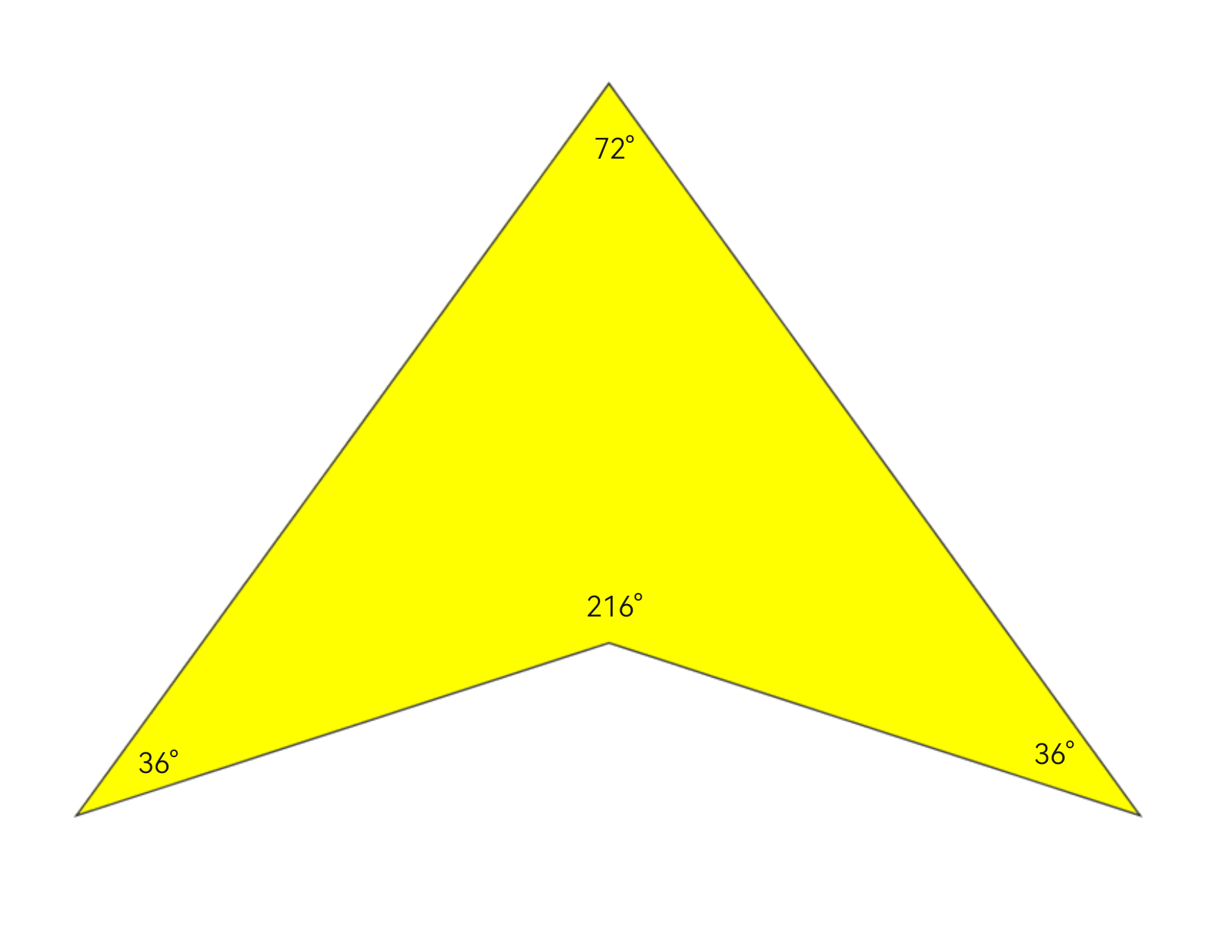
(a) Dart tile

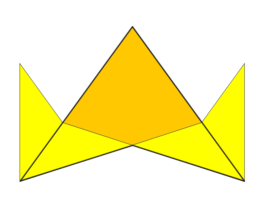
(b) Dart tile after substitution

Figure 2. Dart 1

The kite tile is replaced by two darts and a kite (all three scaled by $1/\Phi$) as follows:

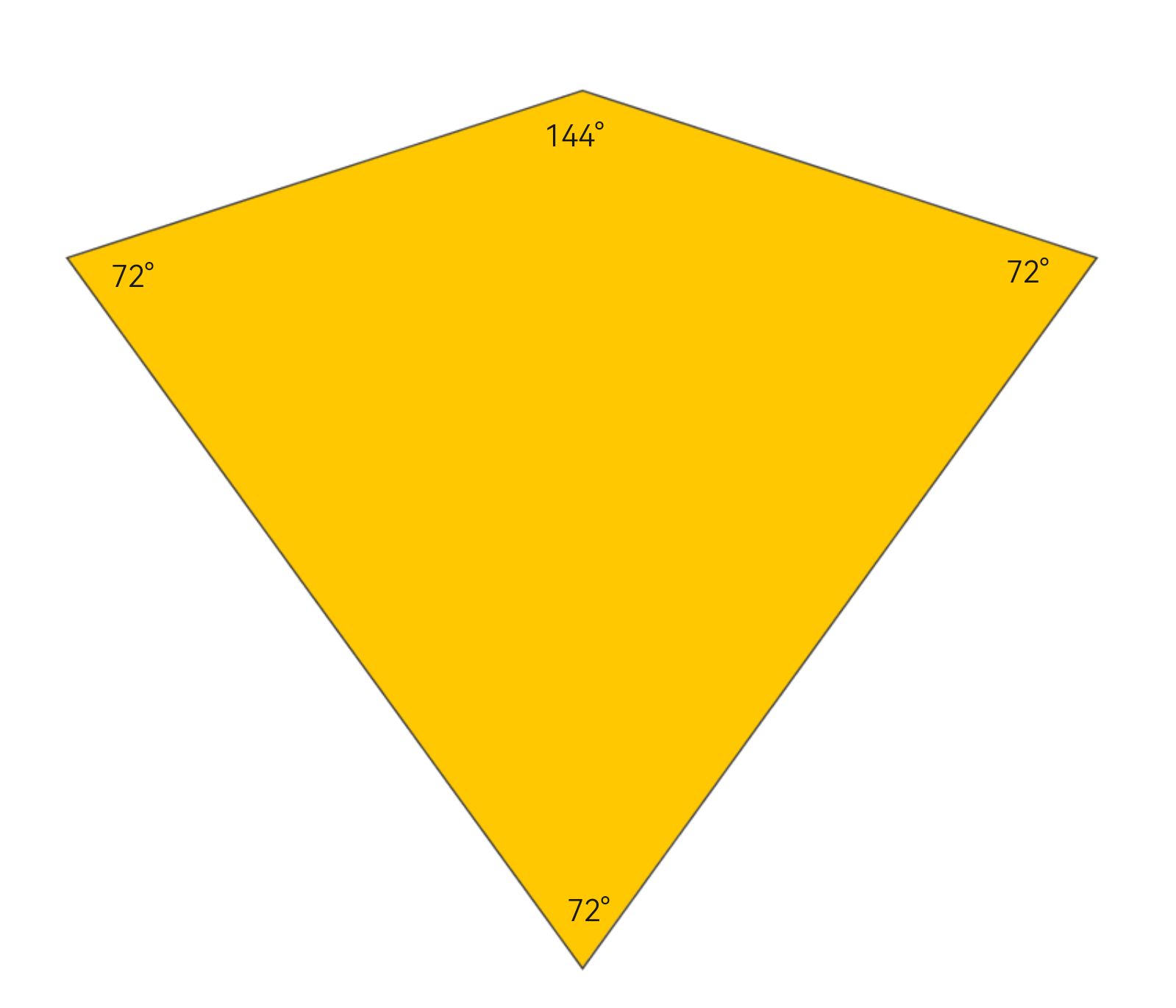
(a) Kite tile

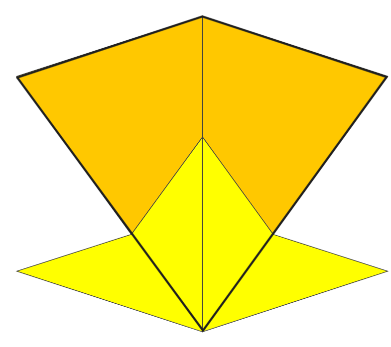
(b) Kite tile after substitution

Figure 3. Kite 1

Here is the image we get when we iterate the substitution starting from the dart tile one more time: that is we perform the substitution process again for the one kite tile and two dart tiles above. We then obtain a collection of kite and dart tiles, scaled by a factor of $1/\Phi^{2}$ from the original kite and dart tiles. Note that we have some perfectly overlapping tiles in this step.

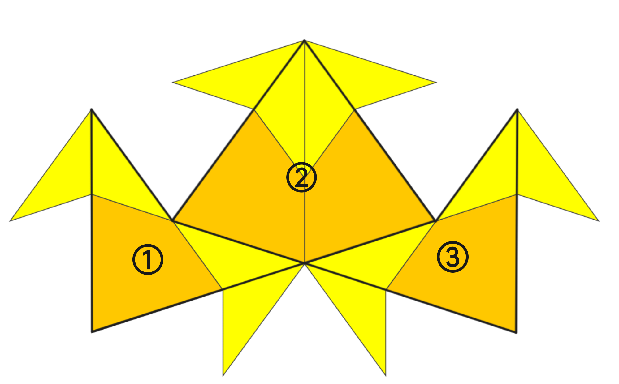
Figure 4. Dart 2

We can of course continue iterating this process to get a tiling like this:

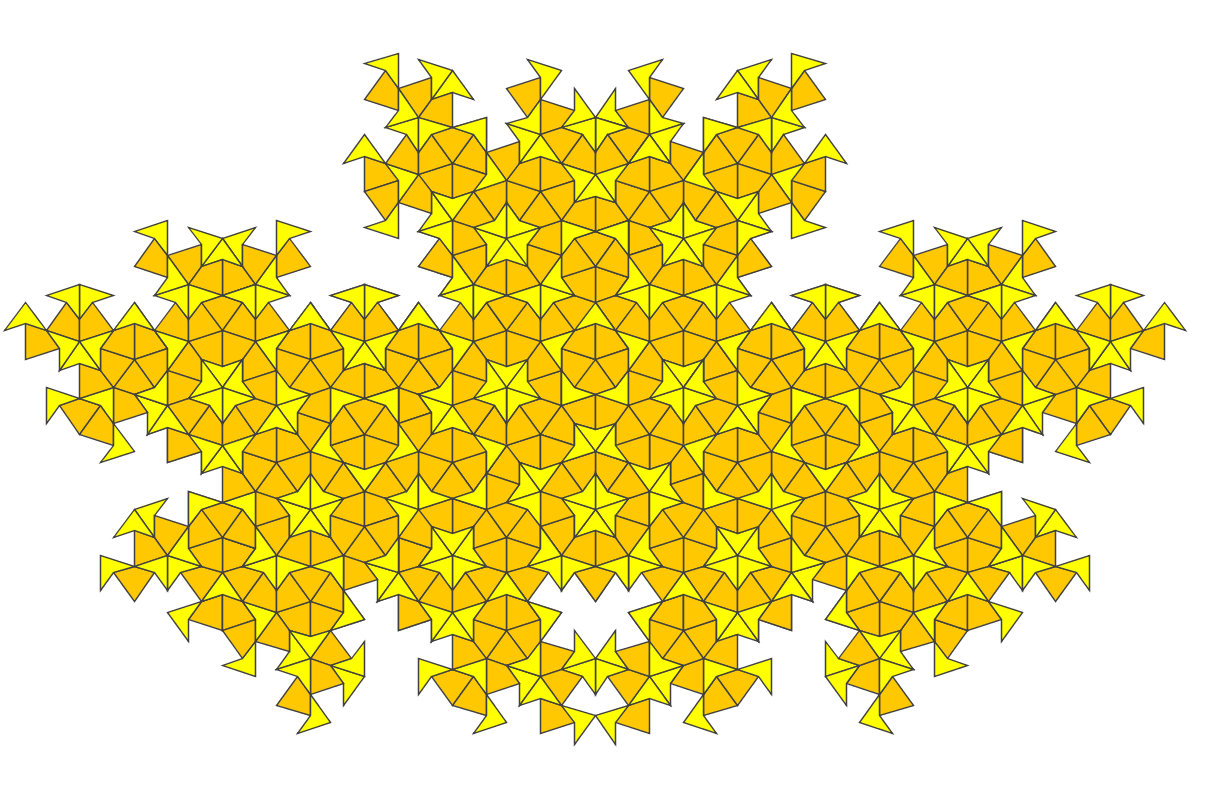
Figure 5. Tiling obtained from iterating the substitution process several times starting with the dart tile

Starting with a kite tile and iterating multiple times results in the following tiling pattern:

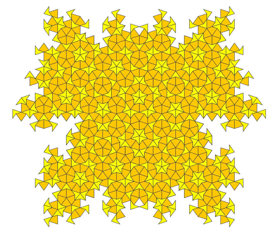
Figure 6. Tiling obtained from iterating the substitution process several times starting with the kite tile

2.1.2. Fat Rhombus & Thin Rhombus

Another type of Penrose tiling is known as the rhombus tiling. This tiling also involves two types of tiles, which are both rhombuses. The fat rhombus tile has interior angles of $72^{\circ}$ and $108^{\circ}$, whereas the thin rhombus tile has interior angles of $36^{\circ}$ and $144^{\circ}$.

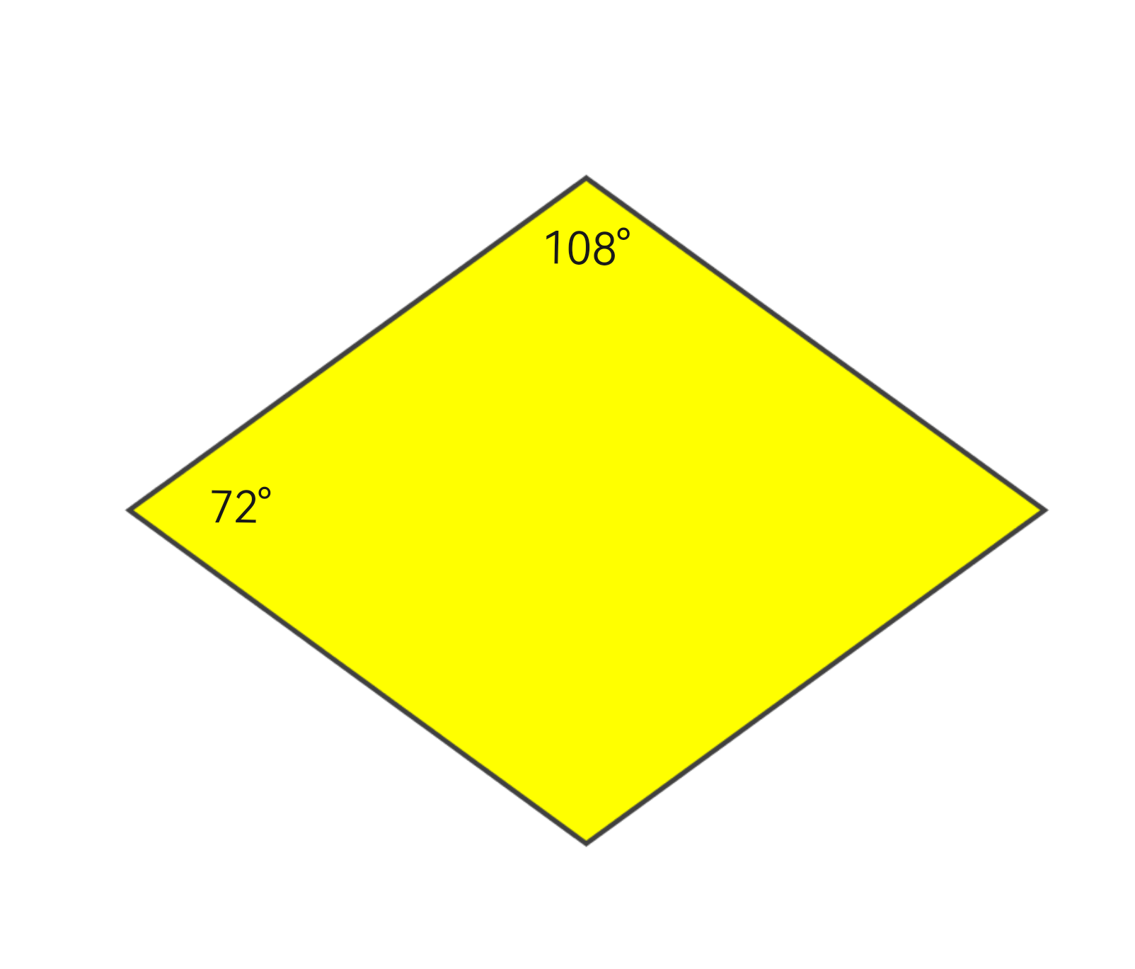
(a) Fat Rhombus

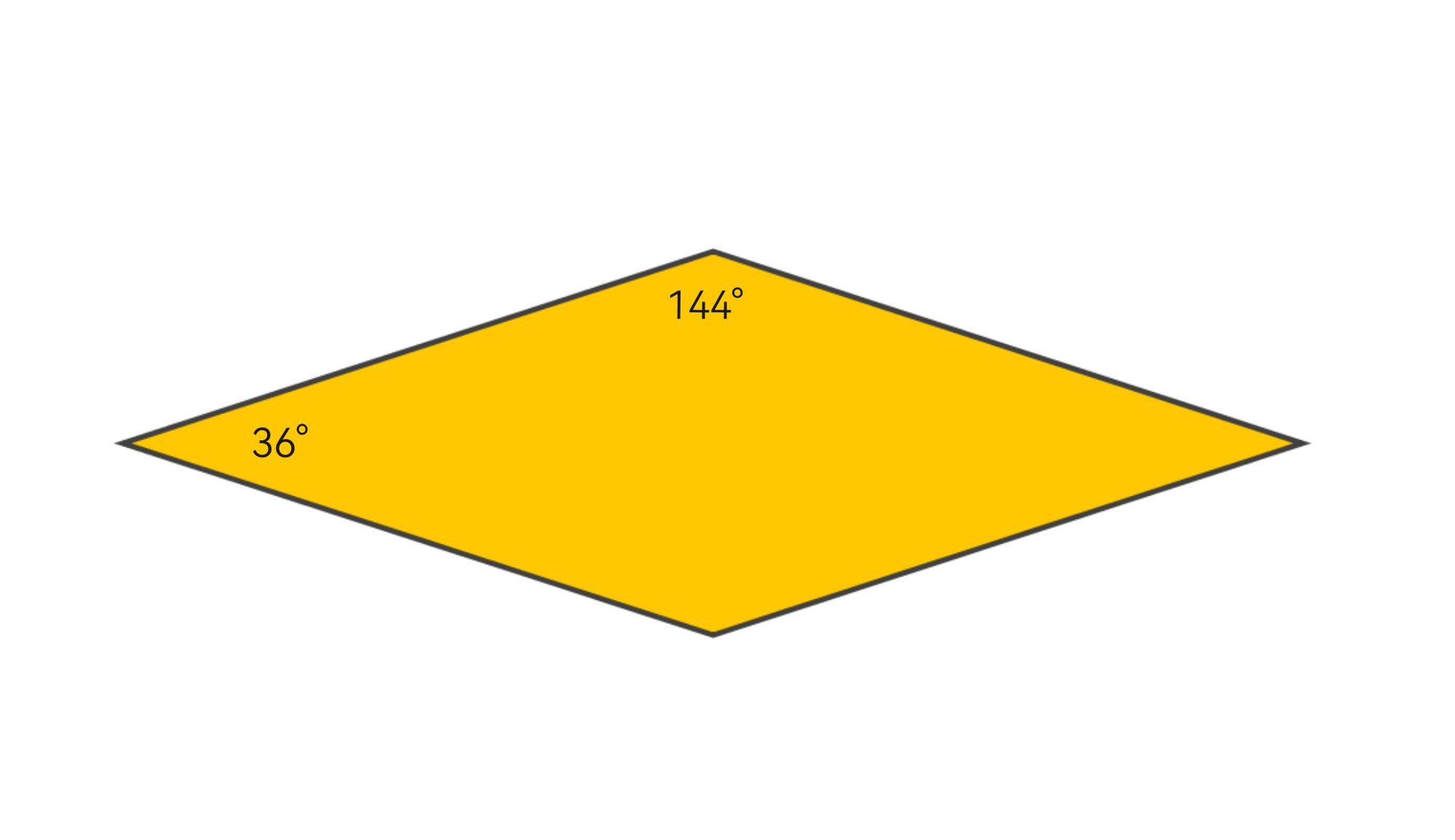
(b) Thin Rhombus

Figure 7. Rhomb 1

The substitution process to generate this rhombus tiling involves replacing a fat rhombus with three fat rhombuses and two thin rhombuses, and replacing a thin rhombus with two fat rhombuses and two thin rhombuses. The substituted tiles are again scaled to $1/\Phi$ the lengths of the original tiles.

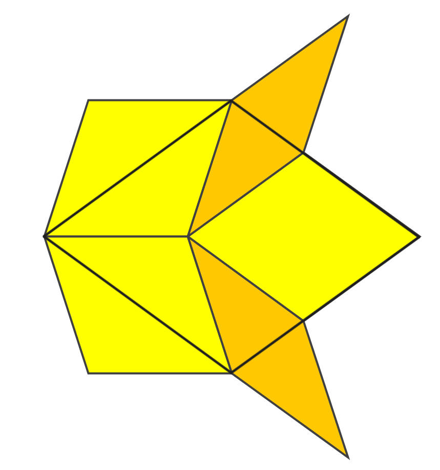
(a) Fat rhombus tile after substitution

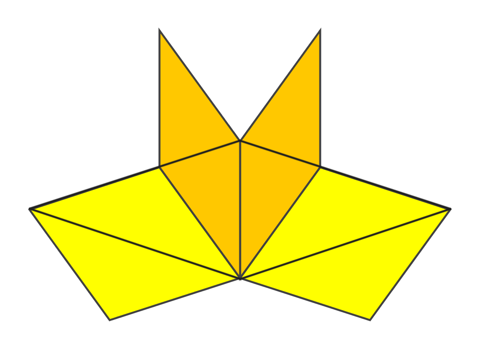
(b) Thin rhombus tile after substitution

Figure 8. Rhomb 2

After several iterations, the tilings are as follows:

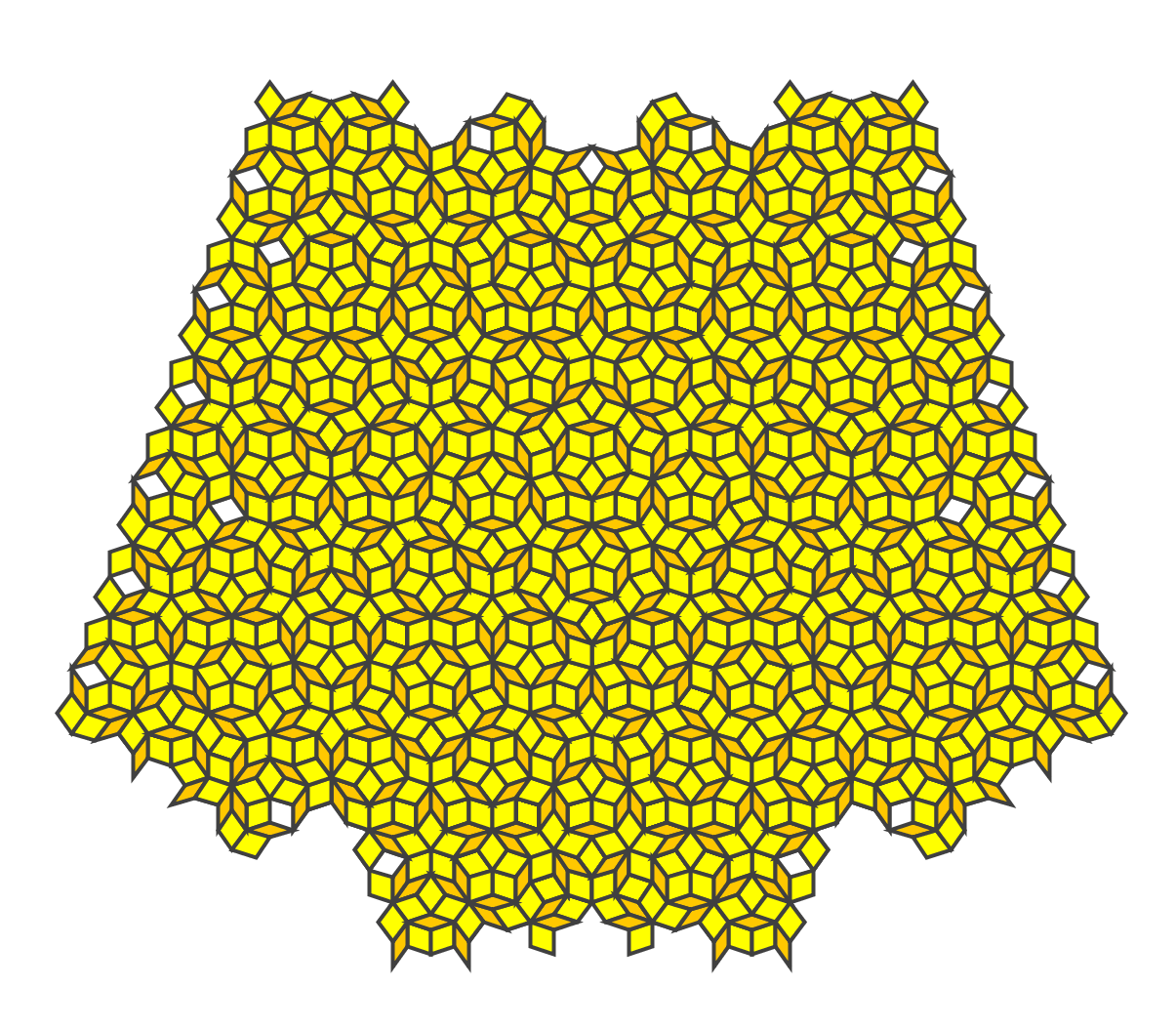
Figure 9. Tiling obtained from iterating the substitution process several times starting with the fat rhombus tile

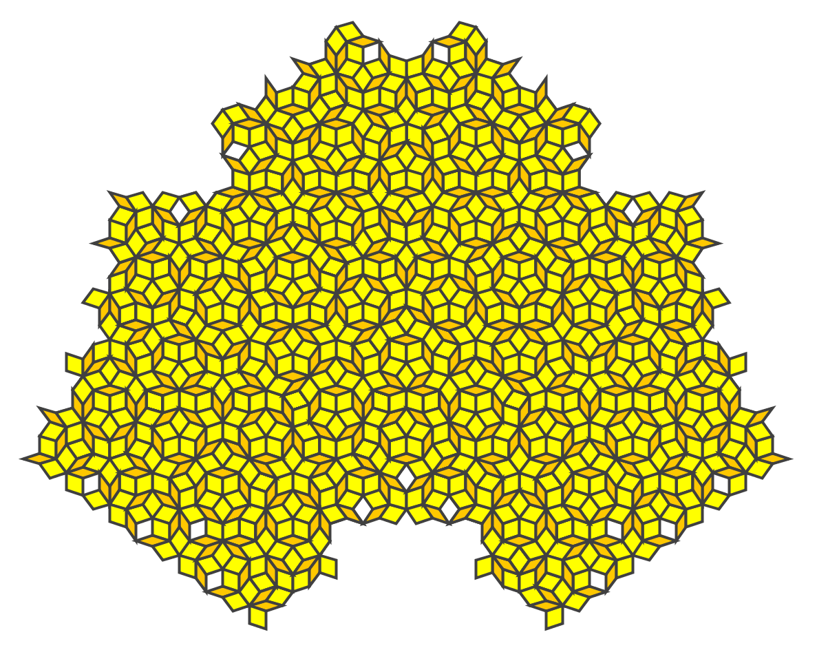
Figure 10. Tiling obtained from iterating the substitution process several times starting with the thin rhombus tile

2.2. Ammann–Beenker tiling

The Ammann Beenker tilings are composed of a rhombus with interior angles $45^{\circ}$ and $135^{\circ}$ and a square. All edges of both tiles have the same length. [BM82].

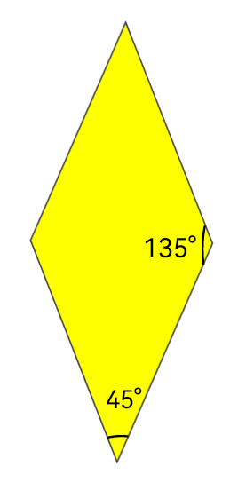
(a) 45-135 Rhombus

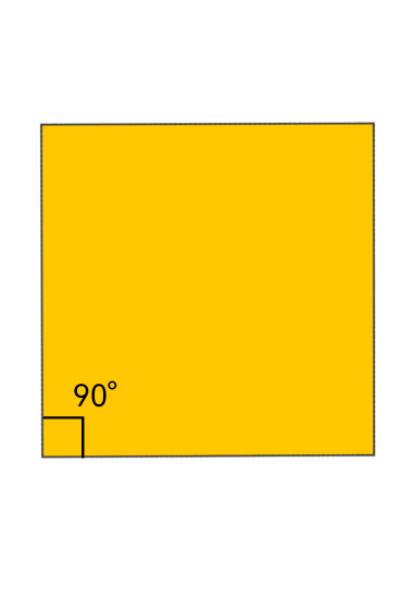
(b) Square

Figure 11. Ammann-Beenker Tilings

Under the Ammann-Beenker substitution rule, the 45-135 degree rhombus is replaced by three rhombuses and four squares, while the square is replaced by four rhombuses and five squares. This time, the substituted tiles are scaled by $1/(1+\sqrt{2})$ compared to the original tiles.

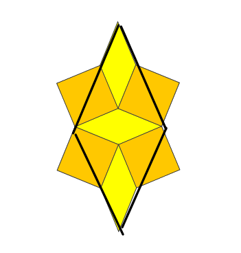
(a) The 45-135 rhombus after one substitution step

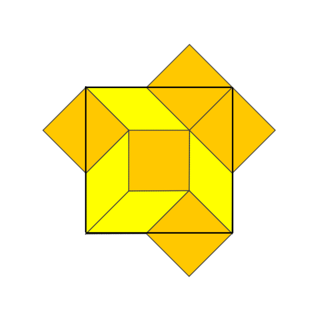
(b) The square after one substitution step

Figure 12. Ammann-Beenker Tilings

Figure 13 illustrates the plane tiling that starts from the 45-135 degree Rhombus

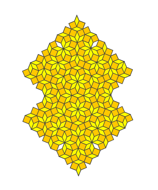
Figure 13. The 45-135 rhombus after several substitution steps

The figure 14 demonstrates the plane tiling that begins from the square.

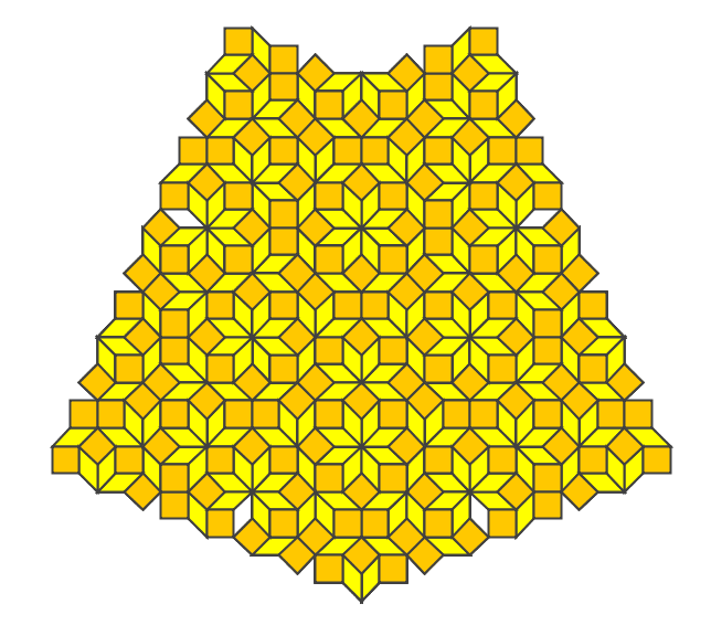
Figure 14. The 45-135 rhombus after several substitution steps

2.3. Ammann A2

The Ammann A2 Tiling was first discovered by Robert Ammann in 1977. [GS87]. This tiling consists of two right-angled irregular hexagons as shown below. The two tilings are of the same shape but different sizes. Let $\Psi=\sqrt{\Phi}$ be the square root of the golden ratio. The small hexagon is a $1/\Psi$ scaled version of the large hexagon.

(a) Small Hexagon

(b) Big Hexagpn

Figure 15. Ammann A2 tiles

The substitution rule for the Ammann A2 tiling proceeds as follows. The small hexagon tile gets replaced by the large hexagon tile. The large hexagon tile gets replaced by a large hexagon and a small hexagon, in an arrangement shown in Figure 16 below. The substituted tiles are scaled $1/\Psi$ compared to the original tiles. All the lengths of the sides of the tiles in every substitution step can be written as a constant times the power of $\Psi$ (we may choose the constant to be $1$) [DSV20].

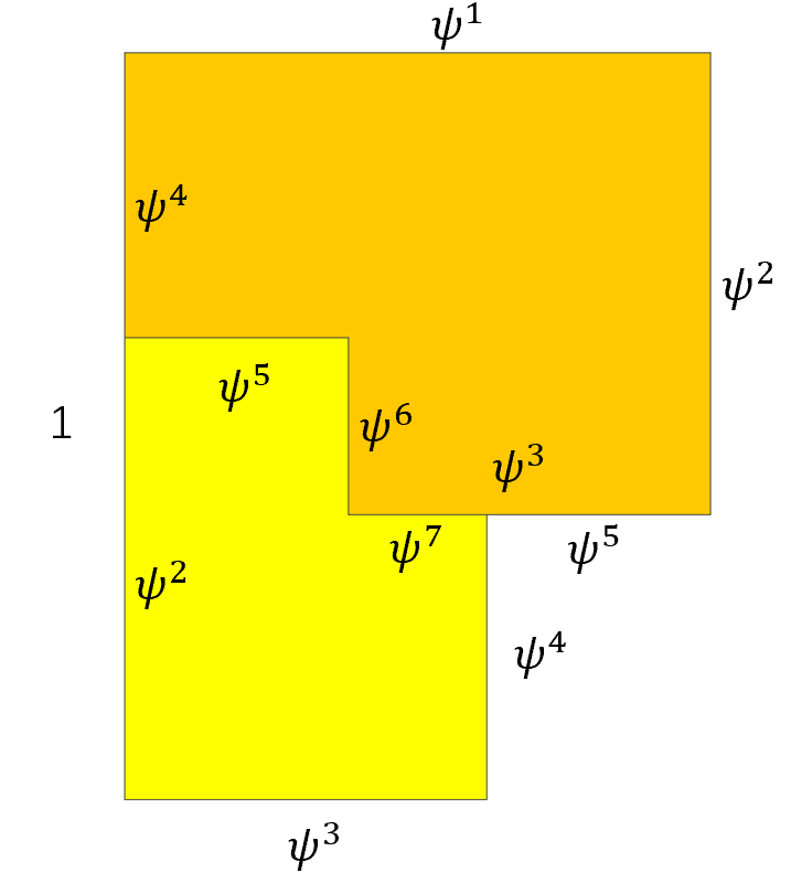
Figure 16. A single large hexagon tile gets replaced by a large hexagon tile and a small hexagon tile, scaled by $1/\Psi$

Notice that, since $\Psi$ is the square root of the golden ratio

(1) $${\Psi}^{4}+{\Psi}^{2}=1$$

Which means,

(2) $${\Psi}^{n+2}/{\Psi}^{n}=\dfrac{\sqrt{5}+1}{2}$$

And

(3) $${\Psi}^{n+4}+{\Psi}^{n+2}={\Psi}^{n}$$

Let us call the tiling obtained from the small hexagon tile after $n$ steps of the substitution algorithm the Generation $n$ Ammann A2 tiling. Then we notice that each new generation of the Ammann A2 tiling is composed of the previous two generations. For instance, the following three generations are illustrated: generation 2, generation 3 and generation 4. Specifically, generation 4 is composed of generation 3 rotated 90 degrees clockwise and generation 2 flipped vertically.

(a) Generation 2

(b) Generation 3

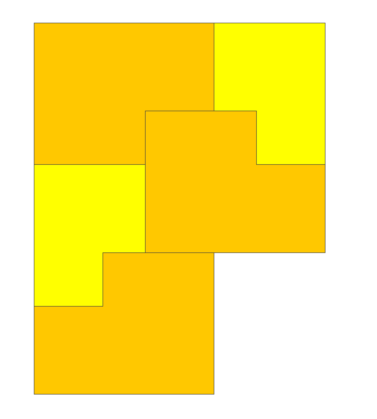
(c) Generation 4

Figure 17. Two new Ammann A2 generations

After the initial placement, continue to apply the substitution rule to each hexagon in the tiling. Each new generation will be composed of elements from the previous two generations, as described.

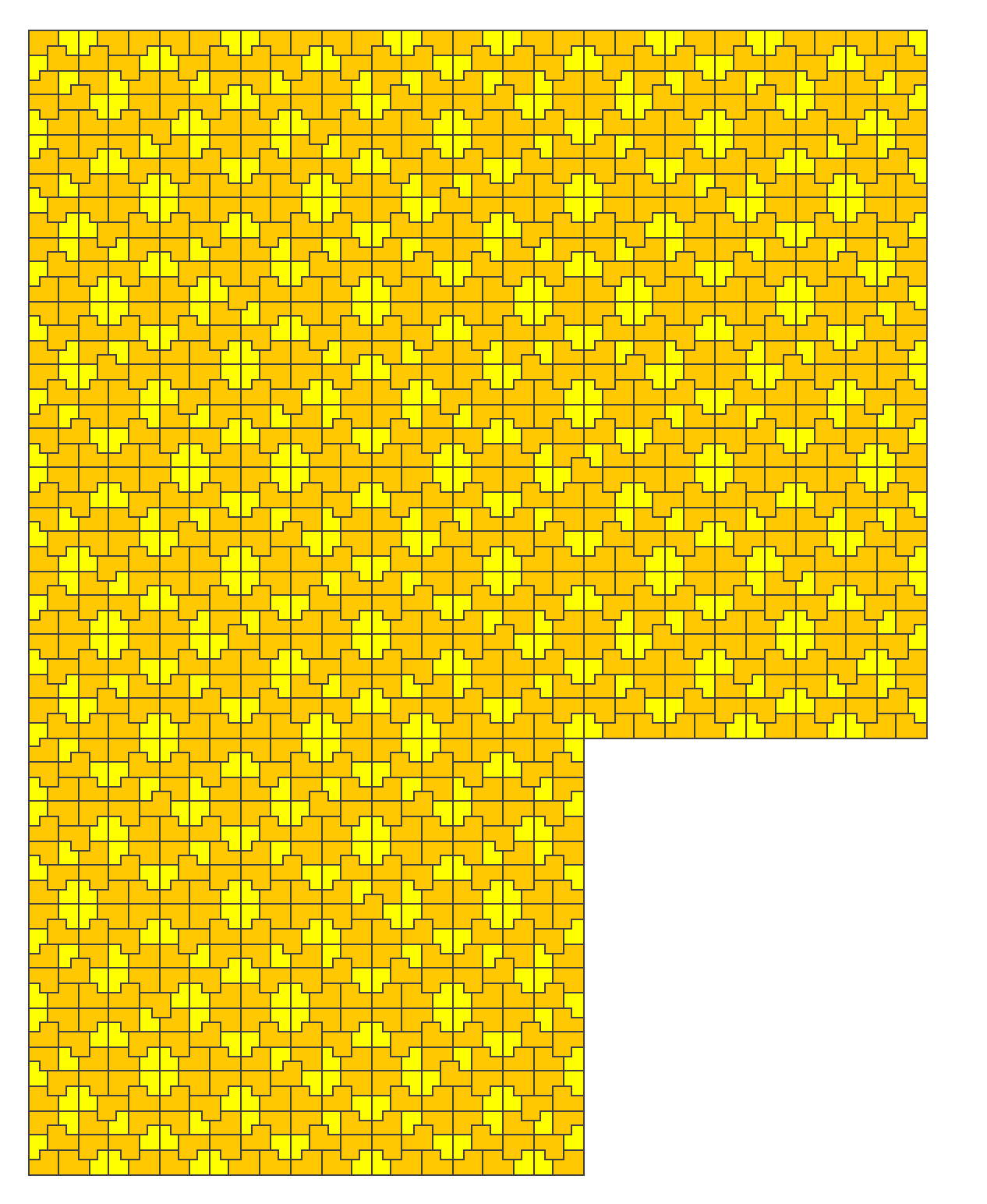
Figure 18. Ammann A2 Set

3. Average degree formula for A2 tiling graph

Given a tiling of a subset of the plane, we may obtain a graph by treating every vertex of a tile as a node, and every straight line boundary of a tile as an edge. The degree of a point is equal to the number of edges connecting to the node. The average degree of a graph can then be calculated as follows. [W⁺01]

(4) $$\text{Average degree of a graph}=\frac{\text{Sum of degrees of all vertices}}{\text{Number of vertices}}$$

We will provide a closed form formula for the average degree of every generation of the Ammann A2 tilings.

3.1. Recursion Formula

For the Ammann A2 tiling, we can determine the average degree of the limiting graph explicitly.

Let us first define F$\left(n\right)$ as the $n$th Fibonacci number, that is [HW79]:

(5) $$F(n)=\dfrac{1}{\sqrt{5}}\cdot\left(\left(\dfrac{1+\sqrt{5}}{2}\right)^{n}-\left(\frac{1-\sqrt{5}}{2}\right)^{n}\right)$$

We will henceforth refer to the $n$th generation of the A2 tiling as the A2-n tiling. Refer to Figures 19(a), 19(b), and 19(c) for pictures of A2-1, A2-2 and A2-3. We then have the following theorem for the average degree of the graph corresponding to the A2-k tiling.

Theorem 1.

Consider the graph corresponding to the A2-$k$ tiling by treating every corner of every tile as a vertex, and every side of every tile as an edge. Let $V(k)$ be the number of vertices in that graph, and let $T(k)$ be the total degree of all the vertices in that graph. Let $F(n)$ be the $n$th Fibonacci number. Then for $k\geq 7$,

(6) $$V(k)=\begin{cases}1+\frac{F\left(\frac{k}{2}\right)}{2}+F\left(\frac{k}{2}+1\right)+2F\left(\frac{k}{2}-1\right)-\frac{F\left(\frac{k}{2}-3\right)}{2}\\ +\left(\frac{31}{2}+\frac{69}{2\sqrt{5}}\right)\left(\frac{1+\sqrt{5}}{2}\right)^{k-7}+\left(\frac{31}{2}-\frac{69}{2\sqrt{5}}\right)\left(\frac{1-\sqrt{5}}{2}\right)^{k-7},&\text{ $k$ even}\\ 1+2F\left(\frac{k+1}{2}\right)+F\left(\frac{k-1}{2}\right)\\ +\left(\frac{31}{2}+\frac{69}{2\sqrt{5}}\right)\left(\frac{1+\sqrt{5}}{2}\right)^{k-7}+\left(\frac{31}{2}-\frac{69}{2\sqrt{5}}\right)\left(\frac{1-\sqrt{5}}{2}\right)^{k-7},&\text{ $k$ odd}\end{cases}$$

and

(7) $$T(k)=\begin{cases}F\left(\frac{k}{2}\right)+2F\left(\frac{k}{2}+1\right)+4F\left(\frac{k}{2}-1\right)-F\left(\frac{k}{2}-3\right)\\ +\left(44+\frac{98}{\sqrt{5}}\right)\left(\frac{1+\sqrt{5}}{2}\right)^{k-7}+\left(44-\frac{98}{\sqrt{5}}\right)\left(\frac{1-\sqrt{5}}{2}\right)^{k-7},&\text{ $k$ even}\\ 4F\left(\frac{k+1}{2}\right)+2F\left(\frac{k-1}{2}\right)\\ +\left(44+\frac{98}{\sqrt{5}}\right)\left(\frac{1+\sqrt{5}}{2}\right)^{k-7}+\left(44-\frac{98}{\sqrt{5}}\right)\left(\frac{1-\sqrt{5}}{2}\right)^{k-7},&\text{ $k$ odd}\end{cases}$$

The average degree of A2-$k$ is then given by $T(k)/V(k)$, and the average degree of the limiting graph is given by

(8) $$\lim_{k\to\infty}\frac{T(k)}{V(k)}=\frac{\left(44+\frac{98}{\sqrt{5}}\right)}{\left(\frac{31}{2}+\frac{69}{2\sqrt{5}}\right)}\approx 2.8396425434090715\ldots.$$

For the sake of completeness, we list $V(k)$ and $T(k)$ for $k=1,2,\ldots 6$ as well. These graphs are small enough that $V(k)$ and $D(k)$ can be counted by hand, using Figures 19(a), 19(b), 19(c), 20(a), 20(b), and 20(c).

Generation, A2-$k$	Vertices $V(k)$	Total Degree $T(k)$
A2-1	6	12
A2-2	6	12
A2-3	9	20
A2-4	12	28
A2-5	18	44
A2-6	26	66

Table 1. Data for A2-1 through A2-6

Before we proceed with the proof of the theorem, let us make some observations about the A2-$k$ graphs.

As previously mentioned, the Ammann A2 tiling follows this rule: the generation $n$ tiling is obtained by combining the $\left(n-1\right)$ th generation and the $\left(n-2\right)$th generation. Therefore, the total number of points and the total degree for the generation $n$ graph are obtained by taking a sum from the graphs corresponding to the previous two generations, adjusted for the changes at the intersection line where the graphs of the previous two generations combine.

If we are focus on the total number of points and the total degrees for the previous two generations, as well as the changes in the degrees and the number of points when combining the previous two generations, we can also calculate the total degree and total number of points for the $n$th generation. Therefore, our task is to identify the changes that occur when combining the previous two graphs. The only change occurs at the common boundary of the two previous generations.

We will henceforth refer to the $n$th generation of the A2 tiling as the A2-n tiling. Let us begin with the A2-1 and A2-2 tilings, each consisting of 6 points and characterized by a total of 12 degrees. To obtain A2-3, we combine the A2-1 and A2-2 tilings. There are four vertices in the intersection line of the A2-1 and A2-2 tilings. We then compare the number of vertices and degrees at those four positions after the two parts are combined, compared to before the two parts are combined.

(a) A2-1

(b) A2-2

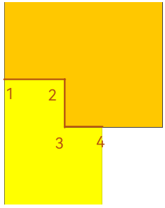
(c) A2-3

Generation	Decrease in		Point No.	Amount
	Vertices	Degree
A2-3	1	1	1	1
	1	2	2 , 3	2
	0	-1	4	1

A2-3 is formed by combining A2-2 tiling rotated 90 degrees and A2-1 tiling flipped vertically. The red intersection line in A2-3 illustrates the changes at each point positions relative to the separated states of A2-1 and A2-2:

• At the No.1 point position, there is a decrease of 1 point and 1 degree compared to when the two parts are separated.

• At the No.2 and No.3 positions, there is a decrease of 1 point and 2 degrees of each.

• At the No.4 position, there is no point reduction because the A2-2 tiling does not contribute a vertex at this position, hence it starts at 0 degrees. The vertex in the A2-1 tiling at the No.4 position, which initially has 2 degrees, increases to 3 degrees after the connection, resulting in a 1 degree increase at this position.

While our table indicates the number of points and degree decreases, it uses -1 to signify an actual increase of 1 degree, as exemplified in the No.4 position.

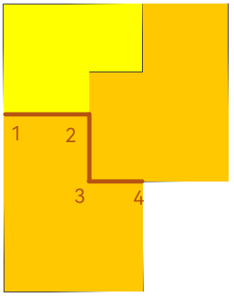
(a) A2-4

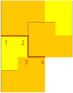
(b) A2-5

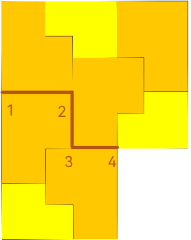
(c) A2-6

Generation	Decrease in		Point No.	Amount
	Point	Degree
A2-4	1	1	1	1
	1	2	2 , 3	2
	0	-1	4	1
A2-5	1	1	1	1
	1	2	2 , 3	2
	0	-1	4	1
A2-6	1	1	1 , 4	2
	1	2	2 , 3	2

Denote the change in the intersection line in a new way:

$\left(change\>in\>point\>number\>,\>change\>in\>degree\>number\right)$ $\times$ $amount$

So the change in A2-4, could be denoted as:  
$\left(1\>,\>1\right)\times 1\qquad\&\qquad\left(1\>,\>2\right)\times 2\qquad\&\qquad\left(0\>,\>-1\right)\times 1$  
Change in A2-5:  
$\left(1\>,\>1\right)\times 1\qquad\&\qquad\left(1\>,\>2\right)\times 2\qquad\&\qquad\left(0\>,\>-1\right)\times 1$  
Change in A2-6:  
$\left(1\>,\>1\right)\times 2\qquad\&\qquad\left(1\>,\>2\right)\times 2$  

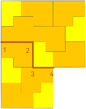
(a) A2-7

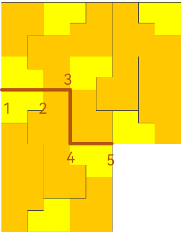
(b) A2-8

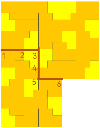
(c) A2-9

Generation	Decrease in		Point No.	Amount
	Point	Degree
A2-7	1	1	1 , 4	2
	1	2	2 , 3	2
A2-8	1	1	1 , 5	2
	1	2	2 , 3 , 4	3
A2-9	1	1	1 , 6	2
	1	2	2 - 5	4

Change in A2-7:  
$\left(1\>,\>1\right)\times 2\qquad\&\qquad\left(1\>,\>2\right)\times 2$  
Change in A2-8:  
$\left(1\>,\>1\right)\times 2\qquad\&\qquad\left(1\>,\>2\right)\times 3$  
Change in A2-9:  
$\left(1\>,\>1\right)\times 2\qquad\&\qquad\left(1\>,\>2\right)\times 4$  

A fundamental rule applies here:  
The points at the two ends always experience a decrease of 1 point and a loss of 1 degree, while the points in the middle section typically decrease by 1 point and lose 2 degrees.  
Concurrently, the number of middle points from A2-7 to A2-9 is gradually increasing: there are 2 middle points in A2-7, 3 in A2-8, and 4 in A2-9.

(a) A2-10

(b) A2-11

(c) A2-12

Generation	Decrease in		Point No.	Amount
	Point	Degree
A2-10	1	1	1 , 8	2
	1	2	2 - 7	6
A2-11	1	1	1 , 9	2
	1	2	2 - 8	7
A2-12	1	1	1 , 12	2
	1	2	2 - 11	10

Change in A2-10:  
$\left(1\>,\>1\right)\times 2\qquad\&\qquad\left(1\>,\>2\right)\times 6$  
Change in A2-11:  
$\left(1\>,\>1\right)\times 2\qquad\&\qquad\left(1\>,\>2\right)\times 7$  
Change in A2-12:  
$\left(1\>,\>1\right)\times 2\qquad\&\qquad\left(1\>,\>2\right)\times 10$  
The change of the two ends are still $\left(1\>,\>1\right)$ and in the middle points are also $\left(1\>,\>2\right)$. The amount of middle points from A2-10 to A2-12 are 6, 7, 10.

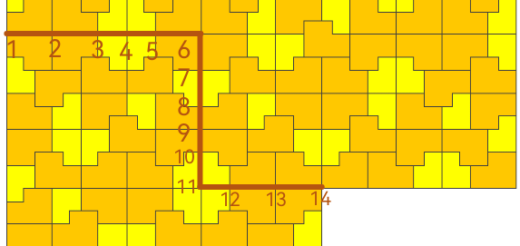
(a) A2-13

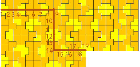
(b) A2-14

Generation	Decrease in		Point No.	Amount
	Point	Degree
A2-13	1	1	1 , 14	2
	1	2	2 - 13	12
A2-14	1	1	1 , 19	2
	1	2	2 - 18	17

Change in A2-13:  
$\left(1\>,\>1\right)\times 2\qquad\&\qquad\left(1\>,\>2\right)\times 12$  
Change in A2-14:  
$\left(1\>,\>1\right)\times 2\qquad\&\qquad\left(1\>,\>2\right)\times 17$  
The change of the middle are still the same but the amount has increased to 12 for A2-13 and 17 for A2-14.

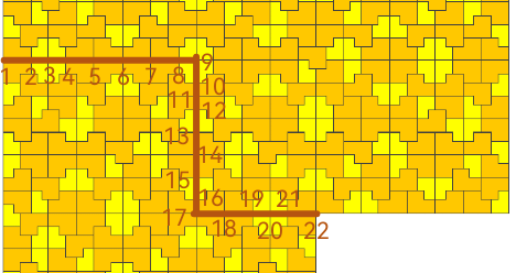
(a) A2-15

Generation	Decrease in		Point No.	Amount
	Point	Degree
A2-15	1	1	1 , 22	2
	1	2	2 - 21	20

The amount of the point in the middle has increased to 20 and the changing way are the same.

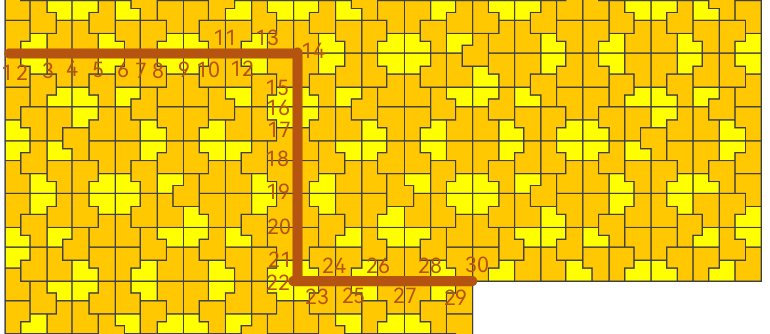
(a) A2-16

Generation	Decrease in		Point No.	Amount
	Point	Degree
A2-16	1	1	1 , 30	2
	1	2	2 - 29	28

Here are 28 points in the middle.

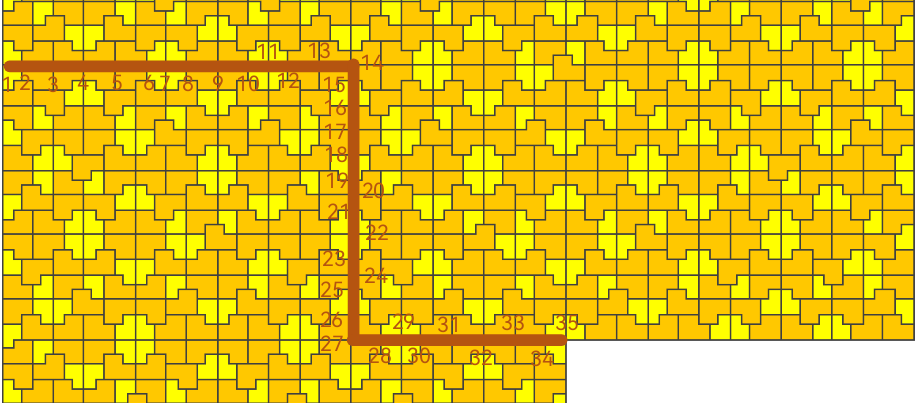
(a) A2-17

Generation	Decrease in		Point No.	Amount
	Point	Degree
A2-17	1	1	1 , 35	2
	1	2	2 - 34	33

In the middle section, there are 33 points.

Starting from A2-7, there are only two types of changes occurring along the intersection line:

• The changes at the two ends: At each end, there is a reduction of 1 point and 1 degree, and this pattern occurs twice $\left(once\>at\>each\>end\right)$.

• The changes in the middle part: There is a decrease of 1 point and 2 degrees. The number of such occurrences varies with each generation.

To discern the underlying rule, consider A2-7 as the first term in the sequence.

A2-7	A2-8	A2-9	A2-10	A2-11	A2-12	A2-13	A2-14	A2-15	A2-16	A2-17
$D_{1}$	$D_{2}$	$D_{3}$	$D_{4}$	$D_{5}$	$D_{6}$	$D_{7}$	$D_{8}$	$D_{9}$	$D_{10}$	$D_{11}$
2	3	4	6	7	10	12	17	20	28	33

Table 2. Relation between generation and amount of middle points

It’s essential to calculate the difference in the number of points between consecutive generations, expressed as $\left(D_{N+1}-D_{N}\right)$, where $D_{N}$ represents the number of points in the Nth generation.

1

1

2

1

3

2

5

3

8

5

Table 3. Differences of middle point amount between two generations

Divide into 2 series $\{a_{n}\}$ and $\{b_{n}\}$ with $a_{n}=D_{2n}-D_{2n-1}$ and $b_{n}=D_{2n+1}-D_{2n}$.

$a_{1}$	$b_{1}$	$a_{2}$	$b_{2}$	$a_{3}$	$b_{3}$	$a_{4}$	$b_{4}$	$a_{5}$	$b_{5}$
1	1	2	1	3	2	5	3	8	5

Table 4. Divide the differences into 2 series

We observe that $\{a_{i}\}$ and $\{b_{i}\}$ are both the Fibonacci sequence. $\{a_{i}\}$ is the Fibonacci sequence from the 2nd term and $\{b_{n}\}$ is the Fibonacci sequence from the 1st term. We will proceed to prove this observation, but we need a lemma first:

Lemma 1.

For the A2-$k$ tiling with $k\geq 9$, any tile $T$ with one of its sides on the intersection line has a dual tile $T^{\prime}$ that is a reflection of $T$ through that side. If $T$ has two sides on the intersection line it has two dual tiles $T^{\prime}$ and $T^{\prime\prime}$, which are reflections of $T$ through those two sides respectively.

Remark. Note that $T$ has to have a full side (with positive length) on the intersection line, if $T$ only has a corner point on the intersection line this lemma does not apply.

Proof.

The A2-9 tiling is small enough that we can verify this lemma is true for it by inspection of Figure 21(c). But then clearly to obtain A2-$k$ for $k\geq 10$, we simply observe that the tile substitution algorithm will create reflection symmetric tiles on both sides of an axis of reflection if the original tiles are reflection symmetric about that axis of reflection. ∎

We are now ready to prove that the $\{a_{k}\}$ and $\{b_{k}\}$ are both Fibonacci sequences.

Lemma 2.

For $k\geq 1$, $a_{k}=F(k+1)$ and $b_{k}=F(k)$, where $F(k)$ is the $k$th Fibonacci number.

Proof.

First, we observe from Figure 19(c) that in the orange tile, the only side where a new point appears after one substitution step is the longest side. From this observation, in Figure 27 we label each side of both the orange and yellow tiles with a number, indicating how many rounds of substitution must occur for a new point to appear on that side.

Figure 27. The numbers labeled on each sides of the tile represent how many substitution steps have to occur before a new point appears on that side.

We then observe in Figure 21(a) that the intersection line there is composed of three sides, which have labels $1,2,3$ according to Figure 27. Similarly Figure 21(b) is composed of four tile sides, with labels $2,4,1,2$. A tile side labeled $1$ gets split into two tile sides, with labels $2$ and $4$

By definition, after one substitution step tile sides with labels $2,3,4,5,6$ or $7$ get their labels reduced by $1$. A tile side with label $1$ splits into two tile sides, with labels $4$ and $2$.

Let $L_{k}$ for $k\geq 7$ represent an unordered list of numbers $1,2,3$ or $4$, which are the labels of the sides on the intersection line of the A2-$k$ tiling. Thus $L_{7}=(1,2,3)$ and $L_{8}=(2,4,1,2)$. To obtain $L_{k+1}$, we start with $L_{k}$ and replace $4\to 3$, replace $3\to 2$, replace $2\to 1$ and replace $1\to 2,4$. Let $|L_{k}|$ represent the length of the list $L_{k}$, so $|L_{7}|=3$ and $|L_{8}|=4$. It is clear that $D_{k}=|L_{k+6}|-1$, since the number of vertices on the intersection line is $1$ plus the number of sides of the intersection line, and $D_{k}$ counts the number of vertices in the intersection line other than the first and the last one. This implies that $a_{k}=D_{2k}-D_{2k-1}=L_{2k+6}-L_{2k+5}$, and $b_{k}=D_{2k+1}-D_{2k}=L_{2k+7}-L_{2k+6}$.

It is clear that for any $k\geq 7$, $L_{k+1}-L_{k}$ is equal to the number of ‘$1$’s in the list $L_{k}$ (since this is the only way a new side can be created). If $k\geq 8$ each ‘$1$’ in $L_{k}$ arises from a ‘$2$’ in $L_{k-1}$, which (if $k\geq 11$) itself arises from either a ‘$1$’ in $L_{k-2}$ or a ‘$1$’ in $L_{k-4}$.

This line of reasoning implies that if $k\geq 3$,

$$a_{k}= L_{2k+6}-L_{2k+5}$$

$$= (\text{number of `$1$'s in $L_{2k+5}$})$$

$$= (\text{number of `$1$'s in $L_{2k+3}$})+(\text{number of `$1$'s in $L_{2k+1}$})$$

(9) $$= a_{k-1}+a_{k-2}.$$

We can similarly show that for $k\geq 3$, $b_{k}=b_{k-1}+b_{k-2}$.

In other words, both $\{a_{k}\}$ and $\{b_{k}\}$ obey the Fibonacci recursion. The sequence $\{b_{k}\}$ has initial conditions $b_{1}=b_{2}=1$, and $\{a_{k}\}$ has initial conditions $a_{1}=1$, $a_{2}=2$. This concludes our proof. ∎

We are now able to write a formula for $D_{k}$ based on the Fibonacci numbers:

Lemma 3.

For $k\geq 3$, $D_{k}=-1+F(\lfloor k/2\rfloor+2)+F(\lfloor(k-1)/2\rfloor)$.

Proof.

Recall the following formula for the sum of the first $n$ Fibonacci numbers (found in, for instance [HW79])

(10) $$\sum_{k=1}^{n}F(k)=F(n+2)-1.$$

We know that $D_{1}=2$, $D_{2}=3$ and for $k\geq 3$ ,

$$D_{k}= D_{1}+\sum_{j=1}^{\lfloor k/2\rfloor}a_{j}+\sum_{i=1}^{\lfloor(k-1)/2\rfloor}b_{i}$$

$$= D_{1}+\sum_{j=1}^{\lfloor k/2\rfloor}F(j+1)+\sum_{i=1}^{\lfloor(k-1)/2\rfloor}F(i)$$

$$= 2+((F(\lfloor k/2\rfloor+3)-1-1)+(F(\lfloor(k-1)/2\rfloor+2)-1)$$

$$= -1+F(\lfloor k/2\rfloor+3)+F(\lfloor(k-1)/2\rfloor+2)$$

∎

Proof of Theorem 1.

The A2-$k$+$2$ tiling is generated by pasting the A2-$k$+$1$ tiling with the A2-$k$ tiling. If $k\geq 7$, we know that $2+D_{k-4}$ of those points will overlap. This implies that for $k\geq 7$

(11) $$V(k+2)=V(k+1)+V(k)-2-D_{k-4}.$$

Using Lemma 3, we know this is equivalent to

(12) $$V(k+2)=V(k+1)+V(k)-1-F(\lfloor(k-4)/2\rfloor+3)-F(\lfloor(k-4-1)/2\rfloor+2).$$

This is a second order non-homogeneous difference equation, and we can apply standard methods to find the general solution. It is not hard to verify the following is a particular solution of (12):

(13) $$V_{p}(k)=\begin{cases}1+\frac{F\left(\frac{k}{2}\right)}{2}+F\left(\frac{k}{2}+1\right)+2F\left(\frac{k}{2}-1\right)-\frac{F\left(\frac{k}{2}-3\right)}{2},&\text{ $k$ even}\\ 1+2F\left(\frac{k+1}{2}\right)+F\left(\frac{k-1}{2}\right),&\text{ $k$ odd}\end{cases}$$

We now find the complementary solution. This is straightforward, because the homogeneous part of (12) is just the Fibonacci recursion equation. We thus have the complementary solution

(14) $$V_{c}(k)=C_{1}\left(\frac{1+\sqrt{5}}{2}\right)^{k-7}+C_{2}\left(\frac{1-\sqrt{5}}{2}\right)^{k-7},$$

for constants $C_{1}$ and $C_{2}$. Given (13) and (14) with initial conditions $V(7)=40,V(8)=61$ (obtained from counting the vertices in Figures 21(a) and 21(b)), we find that the solution of (12) given in (6).

Now we consider $T(k)$. Recall that $T(k)$ refers to the total degree of all vertices in the graph corresponding to A2-$k$. Again, we use the fact that the A2-$k$+$2$ tiling is generated by pasting the A2-$k$+$1$ tiling with the A2-$k$ tiling.

In this pasting process, the only vertices of A2-$k$ and A2-$k$+$1$ that undergo changes in their degree are the ones on the intersection line. Assume that $k\geq 7$. We note that all edges are either horizontal or vertical. Together with Lemma 1 this implies all vertices on the intersection line have degree three or four. The first vertex on the intersection line has degree three, while the other $1+D_{k+2}$ vertices in the intersection each have degree four. Those first and last points on the intersection line of A2-$k+2$ arise from four point in A2-$k$ and A2-$k+1$ (two in A2-$k$ and two in A2-$k+1$) with three of them of degree two and one of them of degree three. The three vertices of degree two appear in two corners of A2-$k$ and one corner of A2-$k+1$, while the one vertex of degree three appears in the interior of one of the sides of A2-$k+1$, and we know the degree there has to be three due to Lemma 1.

Thus before the pasting the four corner points had total degree 9, after the pasting the first and last points on the intersection line have total degree 7. Thus the pasting process results in a loss of $2=9-7$ degrees from the first and last vertices on the intersection line.

We now consider the $D_{k-4}$ middle vertices on the intersection line of A2-$k$+$2$. Before the pasting, each of these $D_{k-4}$ middle vertices arise from a vertex from A2-$k$ and a vertex from A2-$k$+$1$.

From Lemma 1, we can see that after pasting each of the $D_{k-4}$ middle vertices must have degree exactly $4$. Before pasting, the middle vertex corresponds to either two vertices of degree three each in A2-$k$ and A2-$k$+$1$ (this occurs when the vertex is not in a corner of A2-$k$ or A2-$k$+$1$) or one vertex of degree $2$ and one vertex of degree $4$ in A2-$k$ and A2-$k$+$1$ (this occurs when the vertex appears in a corner of A2-$k$ or A2-$k$+$1$).

Thus the pasting process results in a loss of $2D_{k-4}$ degrees from the middle vertices on the intersection line.

From this we can derive a recursion equation for $T(k)$ when $k\geq 7$:

(15) $$T(k+2)=T(k+1)+T(k)-2-2D_{k-4}$$

Using Lemma 3, we know this is equivalent to

(16) $$T(k+2)=T(k+1)+T(k)-2F(\lfloor(k-4)/2\rfloor+3)-2F(\lfloor(k-4-1)/2\rfloor+2).$$

Again, this is a second order non-homogeneous difference equation. We can check that the following is a particular solution of (16):

(17) $$T_{p}(k)=\begin{cases}F\left(\frac{k}{2}\right)+2F\left(\frac{k}{2}+1\right)+4F\left(\frac{k}{2}-1\right)-F\left(\frac{k}{2}-3\right),&\text{ $k$ odd}\\ 4F\left(\frac{k+1}{2}\right)+2F\left(\frac{k-1}{2}\right),&\text{ $k$ even}\end{cases}$$

The homogeneous parts of (12) and (16) are the same, so the complementary solution of (16) is just (14). Using the initial conditions $T(7)=104$, $T(8)=162$ from counting the degrees of vertices in Figures 21(a) and 21(b), we get the solution of $T(k)$ in (7).

It remains to demonstrate the calculation of average degree for the limiting graph as $k\to\infty$. Notice that by (5) both $V(k)$ and $T(k)$ are linear combinations of powers of $\left(\frac{1\pm\sqrt{5}}{2}\right)$. For large $k$, the largest of these terms will be

(18) $$\left(\frac{31}{2}+\frac{69}{2\sqrt{5}}\right)\left(\frac{1+\sqrt{5}}{2}\right)^{k-7}$$

for $V(k)$ and

(19) $$\left(44+\frac{98}{\sqrt{5}}\right)\left(\frac{1+\sqrt{5}}{2}\right)^{k-7}$$

for $T(k)$.

We then have

(20) $$\lim_{k\to\infty}\frac{T(k)}{V(k)}=\frac{44+\frac{98}{\sqrt{5}}}{\frac{31}{2}+\frac{69}{2\sqrt{5}}},$$

as desired. ∎

4. Numerical calculation results

4.1. Linear regression methods

Let us first discuss our numerical results for the Penrose Tilings and the Ammann-Beenker Tiling. We begin with a single tile, and then perform the substitution algorithm $n$ times to generate a generation $n$ tiling of a subset of the plane. We then obtain its corresponding graph. The number of tiles increases exponentially with $n$, and so the graphs also get very large very quickly.

For small $n$, we can perform a brute force calculation of the average degree. Our goal is to find a limiting average value as $n$ goes to infinity. We will use regression analysis to estimate this limiting average degree of the graph as $n$ goes to infinity.

The algorithm modifies existing programs by [Pen24],[Luo18] and[Liu18] intended to draw the tilings to count the degrees instead. We let the program draw a generation $n$ tiling. We modify the program so whenever it draws an edge, it outputs the coordinates of the two points the edge is between. This gives us an output file that is a list of pairs of coordinates. We can then calculate the total number of points by counting how many distinct pairs of coordinates are generated, and we can calculate the average degree by calculating the total number of edges drawn, and dividing by the number of distinct pairs of coordinates.

Since we want to estimate the average degree of the limiting graph as $n$ tends to infinity, it makes sense to ignore boundary points of the tiling. Due to the “missing" tiles on the boundary, vertices on the boundary tiling will have lower degree than they should. Thus to obtain a more accurate count, we will make sure to exclude boundary points from our average.

Let’s take the plane derived from the Penrose Dart tiling as an example. In the program, the variables $\min X$, $\min Y$, $\max X$, and $\max Y$ correspond to the maximum/minimum $x$ and $y$ coordinates of all points generated in the tiling. We then only include the degrees of the points in the red rectangle region in our calculation for the average degree, thus excluding almost all the boundary points. This red rectangle’s length will be $(\max X-\min X)/3$, and its height will be $(\max Y-\min Y)/3$.

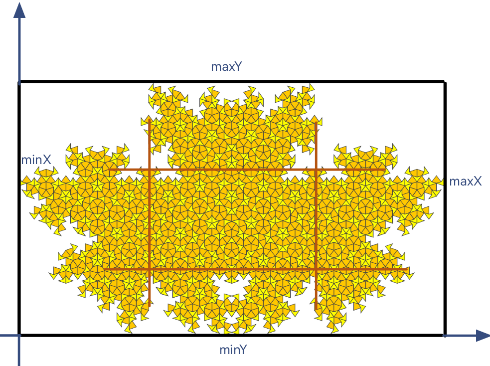
Figure 28. Excluding boundary points

4.1.1. Regression

We then have a numerical calculation for the average degree for the graph corresponding for a generation $n$ tiling, for several $n$. We now use linear regression to estimate the average degree for a limiting graph as $n$ tends to infinity.  
We have data that illustrate the average degrees of graphs for various generations. These data sets are presented as follows:  

Generation	Average Degree
1	$d_{1}$
2	$d_{2}$
3	$d_{3}$
⋮	⋮
n	$d_{n}$

Table 5. Original Data Form

We would want the sequence of average degrees to converge so we can assert that the limiting graph has a definitive average degree value. If we wish to establish a model to capture the relationship between generation and average degree, it would have to be a non-linear regression due to the nature of the data. However, transforming this into a linear regression could be more advantageous for analysis.

To achieve this, we should explore the relationship between $d_{i}-d_{i-1}$ and $d_{i}$, where $d_{i}$ represents the average degree at the ith generation. As $d_{i}-d_{i-1}$ approaches 0, the corresponding $d_{i}$ is expected to approach the average degree of the limiting graph. The independent variable and dependent variable are represented as follows:  

Independent Variable	Dependent Variable
$d_{1}-d_{0}$	$d_{1}$
$d_{2}-d_{1}$	$d_{2}$
$d_{3}-d_{2}$	$d_{3}$
⋮	⋮
$d_{n}-d_{n-1}$	$d_{n}$

Table 6. Data Form - Differences

The following R-code is used to fit the linear model in the form of $y=ax+b$  

⬇

1 deg <- read.table("DifPRF.txt", header = TRUE, sep = "")

2 attach(deg)

3 X = seq(0,0.3,0.00001)

4 deg.model <- nls(y ~ a*x+b, start = list(a = -3, b = 3.8))

5 summary(deg.model)

Listing 1: Sample R Code

4.2. Penrose Tiling

4.2.1. Penrose Tiling - Dart

The dataset of the Penrose Tiling Dart output by the program PenroseTilingDart is written by modifying the program in [Pen24].

Generation	Central Average Degree
1	2.33333
2	2.125
3	2.57778
4	2.75385
5	3.00885
6	3.20316
7	3.38112
8	3.51821
9	3.62899

Table 7. Penrose Dart - Central Average Degree

The rapid increase in average degree suggests using linear regression to estimate its convergence, with calculations starting from the 3rd generation.

$d_{n}-d_{n-1}$ $\left(y\right)$	$d_{n}$ $\left(x\right)$
0.45278	2.57778
0.255	3.00885
0.19431	3.20316
0.17796	3.38112
0.13709	3.51821
0.11078	3.62899

Table 8. Penrose Dart Linear Regression Data

The fitting linear equation is:

(21) $$y=-3.03555x+3.89151$$

The circles in the plot show the data point and the line is the fitting equation .

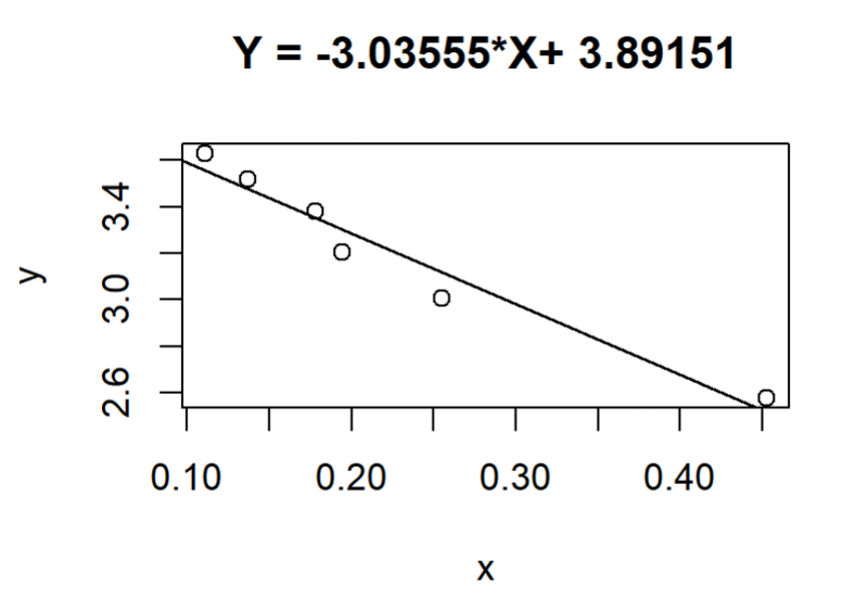
Figure 29. Fitting Plot of Penrose Dart

The convergent average degree is indicated when the difference between successive generations’ average degrees approaches zero, with the y-axis intercept at $x=0$ representing this value. For Penrose tiling initiated from a single dart tile, this convergent degree is calculated to be 3.892.

4.2.2. Penrose Tiling - Kite

The dataset of the Penrose Tiling Kite output by the program PenroseTilingKite is written by modifying the program in [Pen24].

Generation	Central Average Degree
1	2.66667
2	2.85714
3	2.67857
4	2.91391
5	3.0995
6	3.29615
7	3.44794
8	3.5729
9	3.67019

Table 9. Penrose Kite - Central Average Degree

Utilizing data commencing from the 5th generation, we proceed with our analysis.

$d_{n}-d_{n-1}$ $\left(y\right)$	$d_{n}$ $\left(x\right)$
0.19665	3.29615
0.15179	3.44794
0.12496	3.5729
0.09729	3.67019

Table 10. Penrose Kite Linear Regression Data

The fitting linear equation is:

(22) $$y=-3.81617x+4.04126$$

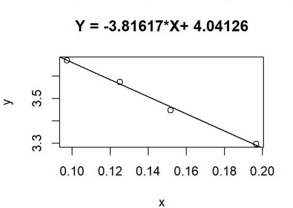
Figure 30. Fitting Plot of Penrose Kite

The calculations reveal that the average degree of a plane starting from a Penrose Tiling kite is 4.042.  

4.2.3. Penrose Tiling - Fat Rhombus

The dataset of the Penrose Tiling Fat Rhombus output by the program PenroseTilingFatRhombus is written by changing program in [Luo18].

Generation	Central Average Degree
1	2.14286
2	2.90909
3	3.12676
4	3.36364
5	3.56929
6	3.69714
7	3.79736
8	3.86685

Table 11. Penrose Fat Rhombus - Central Average Degree

We start to use the data from generation 3.

$d_{n}-d_{n-1}$ $\left(y\right)$	$d_{n}$ $\left(x\right)$
0.23688	3.36364
0.20565	3.56929
0.12785	3.69714
0.10022	3.79736
0.06949	3.86685

Table 12. Penrose Fat Rhombus Linear Regression Data

The fitting linear equation is:

(23) $$y=-2.74563x+4.06526$$

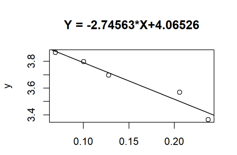
Figure 31. Fitting Plot of Penrose Fat Rhombus

The average degree of the plane starting from a Penrose Tiling kite is 4.066.

4.2.4. Penrose Tiling - Thin Rhombus

The dataset of the Penrose Tiling Thin Rhombus output by the program PenroseTilingThinRhombus is written by changing program in [Luo18].

Generation	Central Average Degree
1	2.5
2	2.94118
3	3.04918
4	3.30994
5	3.51082
6	3.65562
7	3.7682
8	3.84562

Table 13. Penrose Thin Rhombus - Central Average Degree

We start to use the data from generation 3.

$d_{n}-d_{n-1}$ $\left(y\right)$	$d_{n}$ $\left(x\right)$
0.26076	3.30994
0.20088	3.51082
0.1448	3.65562
0.11258	3.7682
0.07742	3.84562

Table 14. Penrose Thin Rhombus Linear Regression Data

The fitting linear equation is:

(24) $$y=-2.93142x+4.08498$$

Figure 32. Fitting Plot of Penrose Thin Rhombus

The average degree of the plane starting from a Penrose Tiling kite is 4.085.  

4.3. Ammann Beenker Tiling

4.3.1. Ammann Beenker - Square

The dataset of the Ammann-Beenker Square Tiling output by the program AmmannBeenkerSquare is written by changing program in [Liu18].

Generation	Central Average Degree
1	2.5
2	3.14474
3	3.54673
4	3.7759
5	3.89125

Table 15. Ammann Beenker Square - Central Average Degree

We start to use the data from generation 2.

$d_{n}-d_{n-1}$ $\left(y\right)$	$d_{n}$ $\left(x\right)$
0.40199	3.54673
0.22917	3.7759
0.11535	3.89125

Table 16. Ammann Beenker Square Linear Regression Data

The fitting linear equation is:

(25) $$y=-1.21205x+4.03956$$

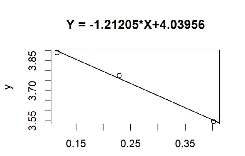
Figure 33. Fitting Plot of Ammann Beenker Square

The average degree of the plane starting from a Ammann Beenker Square is 4.040.  

4.3.2. Ammann Beenker - Rhombus

The dataset of the Ammann-Beenker Rhombus Tiling output by the program AmmannBeenkerRhombus is written by changing program in [Liu18].

Generation	Central Average Degree
1	2.4
2	3
3	3.46369
4	3.73123
5	3.86917

Table 17. Ammann Beenker Rhombus - Central Average Degree

We start to use the data from generation 2.

$d_{n}-d_{n-1}$ $\left(y\right)$	$d_{n}$ $\left(x\right)$
0.46369	3.46369
0.26754	3.73123
0.13794	3.86917

Table 18. Ammann Beenker Rhombus Linear Regression Data

The fitting linear equation is:

(26) $$y=-1.25440x+4.05146$$

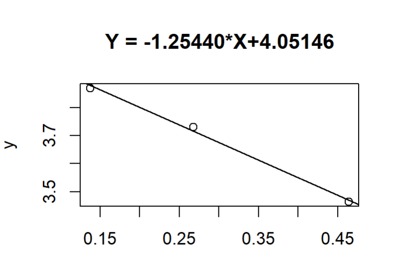
Figure 34. Fitting Plot of Ammann Beenker Rhombus

The average degree of the plane starting from a Ammann Beenker Rhombus is 4.052.

The average degree of all the tilings we discussed before is summarized below:

Sets		Average Degree
Penrose Kite and Dart	Dart	3.892
	Kite	4.042
Penrose Fat and Thin Rhombus	Fat Rhomb	4.066
	Thin Rhomb	4.085
Ammann Beenker	Square	4.040
	Rhombus	4.052

Table 19. Average Degree Summary

Appendix A C++ Programing for central average degree

The code of C++ program in the link:C  
https://github.com/xinyan-x84/FYP/blob/main/FTRhombCen.cpp is shown as following.  

⬇

1#include<iostream>

2#include<fstream>

3#include<iomanip>

4

5using namespace std;

6

7double arr[35000000][3],FT[35000000][3];

8int main(){

9 ifstream inputfile;

10 inputfile.open("D:/FYP/FYP2/PenroseTiling/FatAndThin/Fat/Degree/F3.txt");

11

12 double x,y,AverDeg,PointNum=0, TotalLine = 0, PointNum2=0;

13 int Count=0,Count2=0;

14

15 double maxX=0,maxY=0,minY=10000,minX=10000,KX,KY;

16 while(inputfile>>x>>y){

17 if(x==0 && y==0)

18 break;

19 if(x>maxX)

20 maxX=x;

21 if(y>maxY)

22 maxY=y;

23 if(y<minY)

24 minY=y;

25 if(x<minX)

26 minX=x;

27 arr[Count][0]=x;

28 arr[Count][1]=y;

29 arr[Count][2]=Count/4+1;

30 Count++;

31 }

32 KX=(1/3)*(maxX-minX); KY=(maxY-minY)*(1/3);

33

34 for(int i=0;i<Count;i+=4){

35 for(int j=0;j<Count;j+=4)

36 {

37 if(arr[i][0]==arr[j][0]&&arr[i][1]==arr[j][1]&&

38 arr[i+1][0]==arr[j+1][0]&&arr[i+1][1]==arr[j+1][1]&&

39 arr[i+2][0]==arr[j+2][0]&&arr[i+2][1]==arr[j+2][1]&&

40 arr[i+3][0]==arr[j+3][0]&&arr[i+3][1]==arr[j+3][1]&&

41 arr[i][2]!=arr[j][2])

42 for(int k=0;k<4;k++)

43 {

44 arr[j+k][0]=0;

45 arr[j+k][1]=0;

46 arr[j+k][2]=0;

47 }

48 }

49 }

50for(int i=0;i<Count;i++){

51 for(int j=0;j<=Count2;j++){

52 if(arr[i][0]==FT[j][0] && arr[i][1] == FT[j][1]) // && j<Count2)

53 break;

54 if(arr[i][0]==0 && arr[i][1]==0 && arr[i][2]==0)

55 break;

56 if(j==Count2 && arr[i][0]<(maxX-KX) &&arr[i][0]>(minX+KX) && arr[i][1]<(maxY-KY) && arr[i][1]>(minY+KY)){

57 FT[j][0]=arr[i][0];

58 FT[j][1]=arr[i][1];

59 Count2++;

60 break;

61 }

62 }

63}

64 for(int i=0; i<Count2; i++){

65 for(int j=0; j<Count;j++){

66 if(FT[i][0] == arr[j][0] && FT[i][1] == arr[j][1])

67 FT[i][2]+=1;

68 }

69 }

70 for(int i=0;i<Count2;i++){

71 PointNum++;

72 TotalLine += FT[i][2];

73 }

74 AverDeg=TotalLine/PointNum;

75 cout<<"The total line is: "<<TotalLine<<endl;

76 cout<<"The total point is: "<<PointNum<<endl;

77 cout<<"The average degree is: "<<AverDeg<<endl;

78 cout<<"The actual total point is: "<<Count<<endl;

79 inputfile.close();

80 return 0;

81}

Appendix B R Programing for Linear Regression

The code of R program in the link:  
https://github.com/xinyan-x84/FYP/blob/main/AvePenoseThin.R is shown as following.  

⬇

1 deg <- read.table("DifPRF.txt", header = TRUE, sep = "")

2 attach(deg)

3 X = seq(0,0.3,0.00001)

4 deg.model <- nls(y ~ a*x+b, start = list(a = -3, b = 3.8))

5 summary(deg.model)

Appendix C MATLAB Programing

The code of MATLAB program used to check the avergae degree of Ammann-A2 TIling in the link:  
https://github.com/xinyan-x84/FYP/blob/main/inc.m is shown as following.  

⬇

1A = (1+sqrt(5))/2;

2B = (1-sqrt(5))/2;

3V = zeros(1,100);

4T = zeros(1,100);

5D = zeros(1,100);

6for n=1:100

7 if mod(n,2)~=0

8VN = (31/2+69/(2*sqrt(5)))*A^(n-7)+(31/2-69/(2*sqrt(5)))*B^(n-7)+1+2/sqrt(5)*(A^((n+1)/2)-B^((n+1)/2))+1/sqrt(5)*(A^((n-1)/2)-B^((n-1)/2));

9TN = (44+98/sqrt(5))*A^(n-7)+(44-98/sqrt(5))*B^(n-7)+4/sqrt(5)*(A^((n+1)/2)-B^((n+1)/2))+2/sqrt(5)*(A^((n-1)/2)-B^((n-1)/2));

10 else

11VN = (31/2+69/(2*sqrt(5)))*A^(n-7)+(31/2-69/(2*sqrt(5)))*B^(n-7)+1+1/sqrt(5)*(1/2*(A^(n/2)-B^(n/2))+(A^(n/2+1)-B^(n/2+1))+2*(A^(n/2-1)-B^(n/2-1))-1/2*(A^(n/2-3)-B^(n/2-3)));

12TN = (44+98/sqrt(5))*A^(n-7)+(44-98/sqrt(5))*B^(n-7)+1/sqrt(5)*((A^(n/2)-B^(n/2))+2*(A^(n/2+1)-B^(n/2+1))+4*(A^(n/2-1)-B^(n/2-1))-(A^(n/2-3)-B^(n/2-3)));

13 end

14V(n) = VN;

15T(n) = TN;

16D(n) = TN/VN;

17end

References

- [AGS92] Robert Ammann, Branko Grünbaum, and Geoffrey C Shephard. Aperiodic tiles. Discrete & Computational Geometry, 8(1):1–25, 1992.
- [BG13] Michael Baake and Uwe Grimm. Aperiodic order, volume 1. Cambridge University Press, 2013.
- [BG17] Michael Baake and Uwe Grimm. Aperiodic Order: Volume 2, Crystallography and Almost Periodicity, volume 166. Cambridge University Press, 2017.
- [BM82] Franciscus Beenker and Petrus Maria. Algebraic theory of non-periodic tilings of the plane by two simple building blocks: a square and a rhombus. 1982.
- [DBS23] Azadeh Didari-Bader and Hamed Saghaei. Penrose tiling-inspired graphene-covered multiband terahertz metamaterial absorbers. Optics Express, 31(8):12653–12668, 2023.
- [DL17] Basile De Loynes. Random walks on graphs induced by aperiodic tilings. Markov Processes And Related Fields, 23(1):103–124, 2017.
- [DSV20] Bruno Durand, Alexander Shen, and Nikolay Vereshchagin. On the structure of Ammann A2 tilings. Discrete & Computational Geometry, 63:577–606, 2020.
- [FGH24] D. Frettlöh, F. Gähler, and E. Harriss. Tilings encyclopedia. https://tilings.math.uni-bielefeld.de/, accessed 2024.
- [FSP20] Felix Flicker, Steven H Simon, and SA Parameswaran. Classical dimers on Penrose tilings. Physical Review X, 10(1):011005, 2020.
- [GS87] Branko Grünbaum and Geoffrey Colin Shephard. Tilings and patterns. Courier Dover Publications, 1987.
- [HW79] G. H. Hardy and E. M. Wright. An Introduction to the Theory of Numbers. Oxford University Press, 5th edition, 1979.
- [Kog20] Akihisa Koga. Superlattice structure in the antiferromagnetically ordered state in the Hubbard model on the Ammann-Beenker tiling. Physical Review B, 102(11):115125, 2020.
- [LBS+22] Jerome Lloyd, Sounak Biswas, Steven H Simon, SA Parameswaran, and Felix Flicker. Statistical mechanics of dimers on quasiperiodic Ammann-Beenker tilings. Physical Review B, 106(9):094202, 2022.
- [Liu18] Xiaoyu Liu. Escher-style art using aperiodic tilings. Bachelor’s thesis, Mathematics Department, Xiamen University Malaysia, 2018.
- [Luo18] Junkai Luo. A computer programme to generate custom aperiodic tilings. Bachelor’s thesis, Mathematics Department, Xiamen University Malaysia, 2018.
- [MDH+22] Xinran Ma, Yuping Duan, Lingxi Huang, Hao Lei, and Xuan Yang. Quasiperiodic metamaterials with broadband absorption: Tailoring electromagnetic wave by penrose tiling. Composites Part B: Engineering, 233:109659, 2022.
- [Pen74] R. Penrose. The role of aesthetics in pure and applied mathematical research. Bull. Inst. Math. Appl, 1974.
- [Pen79] Roger Penrose. Pentaplexity a class of non-periodic tilings of the plane. The mathematical intelligencer, 2, 1979.
- [Pen24] Penrose tiling - Rosetta code. https://rosettacode.org/wiki/Penrose_tiling?oldid=367297, accessed 2024.
- [SLF24] Shobhna Singh, Jerome Lloyd, and Felix Flicker. Hamiltonian cycles on Ammann-Beenker tilings. Physical Review X, 14(3):031005, 2024.
- [W+01] Douglas Brent West et al. Introduction to graph theory, volume 2. Prentice hall Upper Saddle River, 2001.
- [Xu24] Xinyan Xu. Average degree of graphs derived from various aperiodic tiling patterns. Bachelor’s thesis, Mathematics Department, Xiamen University Malaysia, 2024.