A method for reconstructing the selfenergy from the spectral function

Abstract

A fundamental question about the nature of quantum materials such as High-T_c systems remain open to date- it is unclear whether they are (some variety of) Fermi liquids, or (some variety of) non Fermi liquids. A direct avenue to determine their nature is to study the (imaginary part of the) selfenergy at low energies. Here we present a method to extract this low $\omega$ selfenergy from experimentally derived spectral functions. The method seems suited for implementation with high quality angle resolved photoemission data. It is based on a helpful Theorem proposed here, which assures us that the method has minimal (or vanishing) error at the lowest energies. We provide numerical examples showing that a few popular model systems yield distinguishably different low energy selfenergies.

1 Introduction

In this work we address the basic problem of reconstructing the low energy $\mathrm{Im}\,\Sigma(\vec{k}_{F},\omega)$ from the spectral function $A(\vec{k},\omega)$ inferred from angle resolved photoemission experiments (ARPES). We refer to this as the inversion problem in this work. The ARPES probe of quantum materials [1] is known to play a vital part in our understanding of the important class of strongly correlated materials. The low $\omega$ dependence of this object for $\vec{k}$$\sim$$k_{F}$ is of especial interest in theoretical studies, since reliable high precision measurements, if available, would provide an essential direction in the search for a suitable theory for systems with strong correlations, and possibly also for superconducting states. Physically the low $\omega$ object is directly related to the decay rate of a slightly excited particle near the ground state, and also can be used to infer a significant contribution to the $T$ dependence of the resistivity of the system at low $T$.

1.1 Current status of the inversion problem

At present a few works report such an inversion. Important recent examples are given in Ref. [2, 3]. The original effort of Ref. [2] uses the direct relationship between the spectral function as a function of the self energy:

$$A(\vec{k},\omega)=\frac{-1}{\pi}\frac{\mathrm{Im}\,\Sigma(\vec{k},\omega)}{(\omega+\mu-\varepsilon_{k}-\mathrm{Re}\,\Sigma(\vec{k},\omega))^{2}+(\mathrm{Im}\,\Sigma(\vec{k},\omega))^{2}},$$ (1)

and therefore at a fixed $\omega$ the width of a peak $\Delta k_{w}$ is given by

$$\hbar v^{eff}_{k}\Delta k_{w}\sim 2\mathrm{Im}\,\Sigma(\vec{k},\omega)$$ (2)

where $v^{eff}_{k}$ is a renormalized velocity, so that the left hand side may be roughly estimated from experiments. The inversion problem of reconstructing $\mathrm{Im}\,\Sigma(\vec{k},\omega)$, requires the collation of data from several constant energy sections of the spectra function, termed the momentum distribution curves (MDC). A second method is presented in Ref. [3], who use a novel momentum-energy resolved tunneling method, and demonstrate its working for two dimensional electron systems embedded in a semiconductor. This important class of materials appears to be ideally suited for that method. Another important direction is the study of the broken symmetry superconducting state of cuprate materials. Here the use of MDC’s to extract the selfenergy, was theoretically proposed in Ref. [4] and studied experimentally in Ref. [5].

1.2 A proposal for inversion

The present work discusses a different framework for effecting this inversion, and provides some examples of how it can be used. In the following instead of the imaginary part of the selfenergy $\mathrm{Im}\,\Sigma(\vec{k},\omega)$, we discuss the equivalent but more convenient positive definite spectral density of the selfenergy, obtained from $\rho_{\Sigma}(\vec{k},\omega)=-\frac{1}{\pi}\mathrm{Im}\,\Sigma(\vec{k},\omega)$. We begin with an exact but apparently infrequently used [6] relation

$$\rho_{\Sigma}(\vec{k},\omega) = \frac{A(\vec{k},\omega)}{\{\Phi_{\vec{k}}(\omega)\}^{2}+\{\pi A(\vec{k},\omega)\}^{2}}$$ (3)

$$\Phi_{\vec{k}}(\omega) \equiv \mathchoice{{\vbox{\hbox{$\textstyle-$}}\kern-4.86108pt}}{{\vbox{\hbox{$\scriptstyle-$}}\kern-3.25pt}}{{\vbox{\hbox{$\scriptscriptstyle-$}}\kern-2.29166pt}}{{\vbox{\hbox{$\scriptscriptstyle-$}}\kern-1.875pt}}\!\int d\nu\frac{A(\vec{k},\nu)}{\omega-\nu}$$ (4)

where $A(\vec{k},\omega)$ is the ARPES related spectral function, $\Phi_{\vec{k}}(\omega)$ is the real part of the Greens function Eq. (33), and $\mathchoice{{\vbox{\hbox{$\textstyle-$}}\kern-4.86108pt}}{{\vbox{\hbox{$\scriptstyle-$}}\kern-3.25pt}}{{\vbox{\hbox{$\scriptscriptstyle-$}}\kern-2.29166pt}}{{\vbox{\hbox{$\scriptscriptstyle-$}}\kern-1.875pt}}\!\int$ represents a principal value integration (see Appendix (A) for details). We see from Eq. (3, 4) that $\rho_{\Sigma}(\vec{k},\omega)$ is a functional of $A(\vec{k},\nu)$. Since the overall scale of $A(\vec{k},\omega)$ is usually unknown in experiments, we can only hope to obtain $\rho_{\Sigma}$ up to an overall constant. This information though should be sufficient to answer the main questions studied below. The non-locality (in frequency) of Eq. (4) presents the main obstacle in this route of inversion. Although $A(\vec{k},\omega)$ is experimentally available for a range of $\omega$ near a peak [7], it seems from Eq. (3, 4) that we need more. The Hilbert transform term $\Phi_{\vec{k}}(\omega)$, requires a knowledge of $A(\vec{k},\nu)$ at all $\nu$ in order to determine $\rho_{\Sigma}$ rigorously. Any error in the estimated $\rho_{\Sigma}(\vec{k},\omega)$ therefore arises only from errors in evaluating $\Phi_{\vec{k}}(\omega)$ due to a limited (partial) knowledge of $A(\vec{k},\omega)$.

On closer inspection, we find that the situation is sensitively dependent on the regions of $\vec{k},\omega$ probed. We summarize our observation about achieving highest accuracy in estimating $\rho_{\Sigma}$ as:

Theorem (On Highest Accuracy Inversion).

As the energy is lowered to zero, errors in the Hilbert transform term $\Phi_{\vec{k}}(\omega)$ are of diminishing consequence to $\rho_{\Sigma}(\vec{k},\omega)$.

To understand the origin of this theorem, consider the following. If we allow for an error $\delta\Phi_{\vec{k}}(\omega)$ at a fixed $\vec{k}$ in the estimation of $\Phi_{\vec{k}}(\omega)$, the resulting fractional error in $\rho_{\Sigma}(\vec{k},\omega)$ to the first order is given by

$$\frac{1}{\rho_{\Sigma}(\vec{k},\omega)}\Big{|}\frac{\delta\rho_{\Sigma}(\vec{k},\omega)}{\delta\Phi_{\vec{k}}(\omega)}\Big{|} = 2\sqrt{\frac{\rho_{\Sigma}(\vec{k},\omega)}{A(\vec{k},\omega)}}\sqrt{1-\pi^{2}A(\vec{k},\omega)\rho_{\Sigma}(\vec{k},\omega)}$$ (5)

$$\leq 2\sqrt{\frac{\rho_{\Sigma}(\vec{k},\omega)}{A(\vec{k},\omega)}}.$$ (6)

The upper bound in the second line is obtained using the observation that Eq. (3) is maximized by dropping $\Phi_{\vec{k}}(\omega)$. In Fig. (1) we illustrate the fractional error and its upper bound given in Eq. (5, 6) for the Asymmetric- Fermi-liquid model Eq. (11) defined below. For $\vec{k}$$\sim$$\vec{k}_{F}$ and $\omega$$\sim$$0$, the spectral function $A(\vec{k},\omega)$ has a peak, and the selfenergy term $\rho_{\Sigma}(\vec{k},\omega)$ is expected to vanish at $T=0$ in disorder-free Fermi systems. The expression Eq. (5) can also be written as $2|\mathrm{Re}\,G(\vec{k},\omega)|\frac{\rho_{\Sigma}(\vec{k},\omega)}{A(\vec{k},\omega)}$, which provides further understanding of the vanishing at $\omega=0$, in terms of the expected vanishing of $\mathrm{Re}\,G(\vec{k}_{F},\omega\sim 0)$. The cumulative effect is that the fractional error and its upper bound Eq. (6) are least in the low energy regime. This regime is also the most interesting one from a physical standpoint, since it defines the asymptotic low energy physics of the system, where the behavior of the selfenergy is an important characterization of the physics of the system. Therefore the above theorem provides a strong motivation to explore the approximate evaluation of Eq. (3), as a way to probe fundamental aspects of interacting Fermi systems.

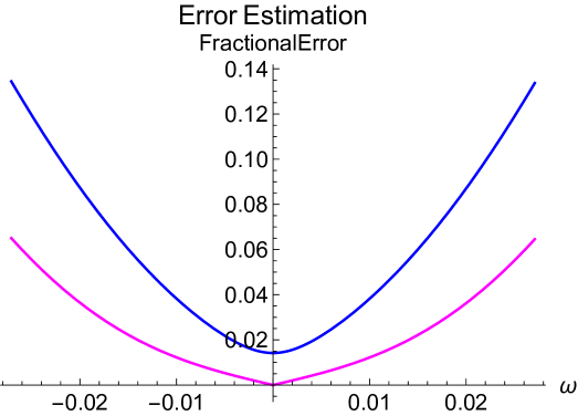
Figure 1: The fractional error Eq. (5) (lower magenta curve) and its upper bound Eq. (6) (upper blue curve) for the Asymmetric Fermi-liquid model Eq. (11) with parameters specified below in Eq. (15). Here $\omega$ is in units of eV as per the model. We note that the bound would also vanish at $\omega=0$ if we use a vanishing elastic scattering energy $\eta$ in Eq. (15).

Encouraged by the above discussion, we propose that this method for extracting the electron selfenergy deserves some experimental effort. We can state our proposal in qualitative terms as follows: at a fixed $\vec{k}$ (chosen say as $\vec{k}_{F}$), the low energy behavior of $\rho_{\Sigma}(\vec{k}_{F},\omega)$, can be found from a knowledge of $A(\vec{k}_{F},\omega)$ in a range of energies sufficiently close to its peak from Eq. (3) supplemented with a suitable frequency windowing of $A(\vec{k}_{F},\omega)$. By frequency windowing we mean replacing $A(\vec{k}_{F},\omega)$ in Eq. (3) as

$$A(\vec{k}_{F},\omega)\to A^{\prime}(\vec{k}_{F},\omega)\equiv{\cal T}(\omega)A(\vec{k}_{F},\omega),$$ (7)

and ${\cal T}(\omega)$ is a smooth symmetric function of $\omega$, falling from 1 to zero smoothly beyond a suitable cutoff energy $\Omega_{*}$. Examples of useful forms of ${\cal T}(\omega)$ are provided below. This procedure can also be carried out for arbitrary $\vec{k}$ away from $\vec{k}_{F}$ with $A^{\prime}(\vec{k},\omega)={\cal T}(\omega-\omega_{\vec{k}})A(\vec{k},\omega)$ where $\omega_{k}$ is the location of the peak in $A(\vec{k},\omega)$.

Clearly the proposal is not rigorous. The possibility of higher order terms in $\delta\Phi_{\vec{k}}$ becoming dominant must be kept in mind while drawing conclusions from the above linear analysis based Theorem. We provide numerical examples below that address this aspect of the problem. The examples displayed below suggest that in certain cases, the procedure leads to a reasonable reconstruction in the low energy regime where it is increasingly accurate- in accordance with the Theorem. In a variety of physically interesting examples, we start with a selfenergy and construct the spectral function from it. We then use the spectral functions cutoff at some energy scale, following the lines suggested in the proposal, from which we reconstruct the selfenergy. Comparing the reconstructed and original selfenergies gives us useful insights. In the examples that are provided, it seems that the presence of a sharp peak in $A(\vec{k},\omega)$ is helpful, as the Theorem Theorem suggests. The utilization of the values of $A(\vec{k},\omega)$ in a range of energies around the peak discussed below, yields an excellent picture of the low energy behavior of the selfenergy.

1.3 The cutoff functions:

We suggested above the use of a windowed version of $A(\vec{k},\omega)$ as in Eq. (7). In choosing to cutoff the frequency at a specific $\Omega_{*}$, typically $\Omega_{*}\sim\nu W_{0}$ i.e. a few times the width of the spectral peak $W_{0}$, we must specify the cutoff function ${\cal T}(\omega)$. In taking the Hilbert transform, it seems useful to consider alternate forms of the cutoff.

We tested a sharp cutoff function

$${\cal T}_{Hard}(\omega)=\Theta(\Omega_{*}-|\omega|)$$ (8)

where $\Omega_{*}$ is the cutoff energy. We also used a cutoff function, inspired by the Tukey window in Fourier transforms, that seems more promising. This piecewise function determined by the cutoff scale $\Omega_{*}$ and two positive numbers $\nu_{-}<\nu_{+}$, in terms of which we define

$${\cal T}(\omega)\Big{|}_{\{\nu_{-}W_{0},\nu_{+}W_{0}\}} = 1\;\mbox{ for }|\omega|<\nu_{-}W_{0}$$ (9)

$$= \frac{1}{2}\left(1+\sin\frac{\pi}{2}\left\{\frac{1+\nu_{+}-2|\omega|/W_{0}}{\nu_{+}-1}\right\}\right)\;$$

$$\mbox{ for }\nu_{-}W_{0}\,<|\omega|<\nu_{+}W_{0}$$

$$= 0\mbox{ for }\nu_{+}W_{0}\leq|\omega|.$$

This function is displayed in Fig. (2). The scale $W_{0}$ is taken in most figures as the width (FWHM) of the spectral function, typical values of the $\nu$ numbers are $\nu_{-}\sim 3$ and $\nu_{+}\sim 6$. Results for both windows are compared below in Fig. (4). While they agree at the lowest energies, in accord with the Theorem, the comparison suggests that the window in Eq. (9) is somewhat better as we go away from $\omega=0$. Without making any claim to its being optimal, we only use the window in Eq. (9) for further results.

2 Examples of selfenergy inversion in three model systems

In order to explore this problem of partial range reconstruction, we study three self energy models next. We also set $\vec{k}=\vec{k}_{F}$ in this part of the work, this is the simplest case where $\Delta k$ in Eq. (27) and Eq. (29) can be set at zero. Calculations for $\vec{k}\neq\vec{k}_{F}$ can be done in exactly the same way, by shifting the peak in the cutoff function Eq. (9) from 0 to $\delta\vec{k}$, the location of the spectral function peak. We comment on this in Fig. (2). Each model is given in terms of an explicit positive definite self energy $\rho_{\Sigma}(\vec{k}_{F},\omega)$ dependent on a few parameters, and having a finite integral over $\omega$.

The three illustrative models considered are expressed (see Eq. (34)) in terms of dimensionless (scaled) frequency $\bar{\omega}\equiv\frac{\omega}{\Omega_{0}}$, a dimensionless temperature $\bar{\tau}=\frac{\pi k_{B}T}{\Omega_{0}}$, a dimensionless interaction strength parameter $\bar{\epsilon}_{0}=\frac{\epsilon_{0}}{\Omega_{0}}$. In the case of the first model we also use $\bar{A}=\frac{A}{\Omega_{0}}$, it is a dimensionless asymmetry parameter. We also use the dimensionless version of $\rho_{\Sigma}$

$$\bar{\rho}_{\Sigma}(\vec{k}_{F},\bar{\omega})=\frac{1}{\Omega_{0}}{\rho}_{\Sigma}(\vec{k}_{F},\omega)$$ (10)

where $\Omega_{0}$ is the “large energy” scale. The relationship between $\Omega_{0}$ and the spectral peak width $W_{0}$ is determined by uninteresting details of the model used. For example changing the confining well from the Gaussian to another form in Eq. (11, 12, 13, 14) would change that relation. Therefore we choose $\Omega_{0}=1$eV and adjust other parameters so that the experimentally observable width (FWHM) $W_{0}$ of the peak at $\omega\sim 0$ is about 10 meV. These peak widths seem to be typical values for the scales for many high T_c materials [1, 2]. The three models, chosen for their proximity to interesting physical cases as well as for analytical tractability in a few cases, are defined by three choices of $\bar{\rho}_{\Sigma}$

$$\mbox{(Asymmetric FL) }\bar{\rho}_{\Sigma}(\vec{k}_{F},\bar{\omega}) = {\epsilon_{0}}\left(\bar{\tau}^{2}+\bar{\omega}^{2}\right)\left(1-\alpha\bar{\omega}\right)e^{-\bar{\omega}^{2}}$$ (11)

$$\mbox{(Marginal-FL-a) }\bar{\rho}_{\Sigma}(\vec{k}_{F},\bar{\omega}) = {\epsilon_{0}}\mbox{Max}[\bar{\tau},|\bar{\omega}|]\;e^{-\bar{\omega}^{2}}$$ (12)

$$\mbox{(Marginal-FL-b) }\bar{\rho}_{\Sigma}(\vec{k}_{F},\bar{\omega}) = {\epsilon_{0}}\left(\bar{\tau}+|\bar{\omega}|\right)\;e^{-\bar{\omega}^{2}}$$ (13)

$$\mbox{(Non-FL) }\bar{\rho}_{\Sigma}(\vec{k}_{F},\bar{\omega}) = {\epsilon_{0}}\left(\bar{\tau}^{\frac{3}{2}}+|\bar{\omega}|^{\frac{3}{2}}\right)e^{-\bar{\omega}^{2}}.$$ (14)

These models are a non-exhaustive subset of the models discussed in literature, and chosen to provide a fairly broad diversity of behaviour. The low frequency behaviour of these models are of especial interest, where the Gaussian term $e^{-\bar{\omega}^{2}}$ is essentially unity. This term is a “confining well”, chosen to provide a fall off at high $\bar{\omega}$ needed for the integrability of the spectral density. Other choices of the confining well are possible but unlikely to make a difference at low $\bar{\omega}\ll 1$, which is the region of our main concern.

In Eq. (11) the chosen Asymmetric FL function (A-FL in the following) describes an asymmetric Fermi liquid, where the first term $(\bar{\tau}^{2}+\bar{\omega}^{2})$ represents a Fermi liquid (FL), while the second term $(1-\alpha\bar{\omega})$ generates a cubic asymmetric term in the self energy. This model is a crude representation of the solution of the  $t$-$J$  model in 2-dimensions using the extremely correlated Fermi liquid theory (ECFL)[9] at the lowest temperatures, if the parameters are chosen appropriately. The resistivity of this model is quadratic in T at the lowest temperature, and crosses over to a T-linear behavior at a very low crossover temperature ([9](d)). This subtle crossover behavior requires the addition of terms of higher order in $\omega$, and is buried in the $T$ dependence of the coefficients. These details are not necessary for the basic analysis here, in this work we will provide a framework from which only the lowest order quadratic behavior- on display in Eq. (11)- might be tested in future experiments. The spectral function can be calculated fully in terms of the Dawson function $D_{F}$ Eq. (44), these and other necessary details are collected in Appendix(B).

In Eq. (12, 13) we consider two variants of the popular marginal Fermi liquid (M-FL in the following) model self energy[10]. As in other models considered, the added exponential term is unity for $|\bar{\omega}|<<1$. The M-FL phenomenology builds in a T linear resistivity in a natural fashion. The model M-FL-b Eq. (13) is in the same spirit as model M-FL-a Eq. (12), and leads to slightly different results at the lowest energy.

In Eq. (14) the chosen non FL function (N-FL in the following) describes a non-Fermi liquid system with a power law $|\omega|^{\frac{3}{2}}$, where the resistivity is expected to behave as $T^{\frac{3}{2}}$. While there appears to be no compelling argument for this specific choice of the power law ${\frac{3}{2}}$ used in our choice, we use it as an archetype of a strongly non Fermi liquid of the type suggested in [11].

We adjust the parameters for these models so that the spectral function has about the same width $W_{0}$ of $\sim 10$meV in all cases.

In summary, in the following we follow these steps:

• For each model we use Eq. (20, 29) to construct $\chi$, and $A(\vec{k},\omega)$.

• We then multiply $A$ with a window function ${\cal T}(\omega)$ in Eq. (9), which vanishes smoothly beyond a frequency scale. This scale is chosen in most cases as $\Omega_{*}$, a suitable multiple of $W_{0}$, the width (FWHM) of the spectral function. This process represents the selection of a small energy window and yields $A^{\prime}$ as in Eq. (7).

• From $A^{\prime}$ replacing $A$ and Eq. (31, 33), we construct $\rho_{\Sigma}(\vec{k},\omega,\Omega_{*})$, which now depends on our choice of $\Omega_{*}$. We then compare with the parent value $\rho_{\Sigma}(\vec{k}_{F},\omega)$, for $|\omega|\ {\raise-2.15277pt\hbox{$\buildrel<\over{\sim}$}}\ \Omega_{*}$.

As a check on the numerics and the formalism, we note that the two self energies must agree when $\Omega_{*}\!\to\!\infty$. We present an example in Fig. (2) to demonstrate this agreement.

2.1 The Asymmetric Fermi liquid model

The parameters defined in Eq. (34) are chosen for the following figures are

$$\epsilon_{0}=1.8,\;\alpha=0.1;\;\eta=0.02;\;\tau=0.02;\;\alpha_{z}=1.74$$ (15)

where $\alpha_{z}$ Eq. (22) corresponds to a filling $n=0.85$, leading to a fairly low value of the quasiparticle weight $Z=0.203$. The energies are given in units of $\Omega_{0}$ chosen to be 1eV for High Tc systems. The value of $\eta$ used here corresponds to typical Laser ARPES experiments [17, 18], while $\tau$, the physical temperature $T=\tau/\pi\sim 74$K. The width (FWHM) of the spectral function at these parameters is $W_{0}$ is $\sim$ 9meV.

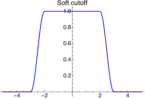
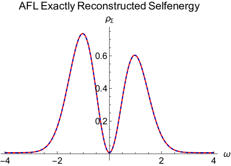
Figure 2: These figures are for the Asymmetric Fermi-liquid model Eq. (11) with parameters given in Eq. (15). Left The soft cutoff function ${\cal T}(\omega)$ in Eq. (9) is illustrated with parameters $\{2,3\}$ and $\Omega_{*}=1$. Right The initial $\rho_{\Sigma}(\vec{k}_{F},\omega)+\frac{\eta}{\pi}$ from Eq. (37, 38) (dotted blue) is exactly reproduced numerically (red), using the full energy window Hilbert transform to evaluate $\mathchoice{{\vbox{\hbox{$\textstyle-$}}\kern-3.88889pt}}{{\vbox{\hbox{$\scriptstyle-$}}\kern-2.6pt}}{{\vbox{\hbox{$\scriptscriptstyle-$}}\kern-1.83333pt}}{{\vbox{\hbox{$\scriptscriptstyle-$}}\kern-1.5pt}}\!\int d\nu\frac{A(\vec{k},\nu)}{\omega-\nu}$ in Eq. (3). It also agrees with the analytical calculation in Eq. (30), showing the consistency of the starting point Eq. (3). A similar calculation performed away from $\vec{k}_{F}$ (as mentioned in the beginning of Section(2)) works equally well.

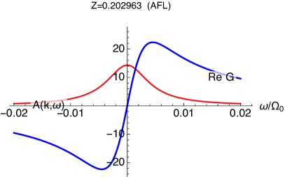
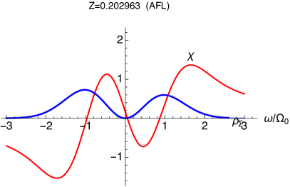
Figure 3: These figures are for the Asymmetric Fermi-liquid model Eq. (11) with parameters given in Eq. (15). (Left) The spectral function $A(\vec{k}_{F},\omega)$ and the $Re\,G(\vec{k}_{F},\omega)$ and (Right) the imaginary self energy $\rho_{\Sigma}(\vec{k}_{f},\omega)$ and $\chi(\vec{k}_{F},\omega)$ for the A-FL model Eq. (11), calculated from Eq. (41, 38, 48), using parameters given in Eq. (15). Here the spectral peak width $W_{0}$ is $\sim$9 meV.

We present figures showing the spectral function and selfenergy for the A-FL model in Fig. (3). We further demonstrate the validity of the basic Eq. (3) for the A-FL model. In Fig. (2) we show the exact reconstruction of the selfenergy from the spectral function using the Hilbert transform over all frequencies.

We present a comparison in Fig. (4) of the reconstruction schemes using two window functions: (a) A hard cutoff ${\cal T}(\omega)=\Theta(3W_{0}-|\omega|)$ at a energy cutoff equaling thrice the FWHM of the spectral peak $W_{0}$ and (b) the soft window given in Eq. (9) with parameters $\{3W_{0},6W_{0}\}$. In the caption we we comment further on the relative merits of the two schemes. In the two figures Fig. (5, 6), we display the reconstructed selfenergy compared to the exact selfenergy for different sets of the cutoff window parameters, and comment on their relative merits.

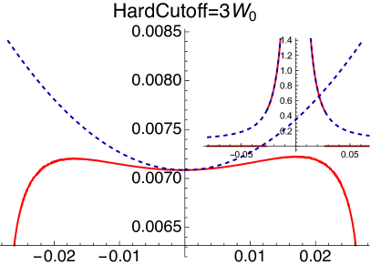
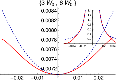
Figure 4: These figures are for the Asymmetric Fermi-liquid model Eq. (11) with parameters given in Eq. (15). The reconstructed selfenergy $\rho_{\Sigma}(\vec{k}_{F},\omega)+\frac{\eta}{\pi}$ (red curve) using on (Left) a hard cutoff Eq. (8) and on (Right) using the soft cutoff Eq. (9) compared with the exact value in the dashed blue curves. The two parameters relating to the soft cutoff Eq. (9) on (Right) are indicated in curly brackets. The two insets show the exact spectral function in dashed blue and the cutoff included spectral function $A^{\prime}$ of Eq. (7) in the red curves. Here $W_{0}$ is $\sim$9 meV. On the (Left), while the hard cutoff does give a shallow minimum near $\omega$$\sim$$0$, it is seen to turn around and become convex rapidly. The soft cutoff remains concave up to $3W_{0}$, and has a maximum (fractional) error of $\sim$6% at the maximum displayed energy $\omega=3W_{0}$.

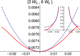
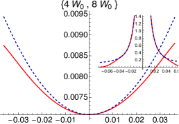
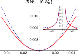
Figure 5: These figures are for the Asymmetric Fermi-liquid model Eq. (11) with parameters given in Eq. (15). The reconstructed selfenergy $\rho_{\Sigma}(\vec{k}_{F},\omega)+\frac{\eta}{\pi}$ (red curves) using the soft cutoff Eq. (9) compared with the exact value in the dashed blue curves. The two parameters relating to the soft cutoff Eq. (9) are indicated in curly brackets. The three insets show the exact spectral function in dashed blue and the cutoff included spectral function $A^{\prime}$ of Eq. (7) in the red curves. Here upper cutoff is twice the lower one. Increasing the magnitude of the cutoff is seen to reduce the error. Here $W_{0}$ is $\sim$9 meV.

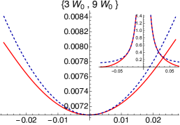
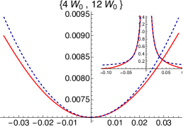
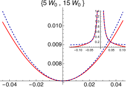
Figure 6: These figures are for the Asymmetric Fermi-liquid model Eq. (11) with parameters given in Eq. (15). The reconstructed selfenergy $\rho_{\Sigma}(\vec{k}_{F},\omega)+\frac{\eta}{\pi}$ (red curves) using the soft cutoff Eq. (9) compared with the exact value in the dashed blue curves. The two parameters relating to the soft cutoff Eq. (9) are indicated in curly brackets. The three insets show the exact spectral function in dashed blue and the cutoff included spectral function $A^{\prime}$ of Eq. (7) in the red curves. Here upper cutoff is 3 times the lower one, and shows a fair improvement over the results of Fig. (5) where the upper cutoff is only twice the lower one. Here $W_{0}$ is $\sim$9 meV.

2.2 The Marginal Fermi liquid model

For the M-FL-a model, the parameters used are

$$\epsilon_{0}=1.8,\eta=0.02,\tau=0.01;\alpha_{z}=1$$ (16)

leading to a width $W_{0}=12$meV, which is only slightly bigger than $W_{0}=9$meV for the A-FL model. The spectral function and the real part of the Greens function are shown in Fig. (7), and the reconstructed selfenergy with a few typical window parameters also in Fig. (7). The reconstructed selfenergy is displayed in Fig. (8).

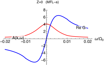
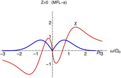
Figure 7: These figures are for the Marginal Fermi Liquid-a model Eq. (12) with parameters given in Eq. (16). (Left) The spectral function $A(\vec{k}_{F},\omega)$ and the $Re\,G(\vec{k}_{F},\omega)$ and (Right) the imaginary self energy $\rho_{\Sigma}(\vec{k}_{f},\omega)$ and $\chi(\vec{k}_{F},\omega)$ for the M-FL-a model Eq. (12), calculated from Eq. (41, 38, 48). Here the spectral peak width $W_{0}$ is $\sim$12meV.

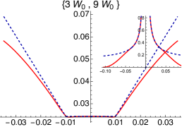
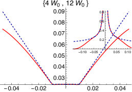
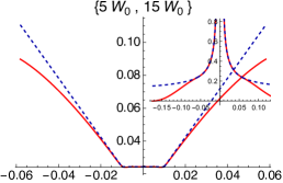
Figure 8: These figures are for the Marginal Fermi Liquid-a model Eq. (12) with parameters given in Eq. (16). The reconstructed selfenergy $\rho_{\Sigma}(\vec{k}_{F},\omega)+\frac{\eta}{\pi}$ (red curves) using the soft cutoff Eq. (9) compared with the exact value in the dashed blue curves. The two parameters relating to the soft cutoff Eq. (9) are indicated in curly brackets. The three insets show the exact spectral function in dashed blue and the cutoff included spectral function $A^{\prime}$ of Eq. (7) in the red curves. Here upper cutoff is 3 times the lower one. Here $W_{0}$ is $\sim$12 meV.

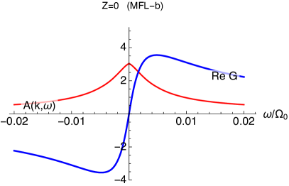
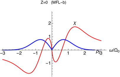
Figure 9: These figures are for the Marginal Fermi Liquid-b model Eq. (13) with parameters given in Eq. (17). (Left) The spectral function $A(\vec{k}_{F},\omega)$ and the $Re\,G(\vec{k}_{F},\omega)$ and (Right) the imaginary self energy $\rho_{\Sigma}(\vec{k}_{f},\omega)$ and $\chi(\vec{k}_{F},\omega)$, calculated from Eq. (41, 38, 48), using parameters given in Eq. (17). Here the spectral peak width $W_{0}$ is $\sim$11meV.

The functional form of $\rho_{\Sigma}$ in the M-FL-a model Eq. (12) has a flat portion in its minima, which is reflected in the lowest energy behaviour as seen in Fig. (8). The M-FL-b model Eq. (13) on the other hand avoids this flat feature. For the M-FL-b model, the parameters used are

$$\epsilon_{0}=1.8,\eta=0.02,\tau=0.015;\alpha_{z}=1$$ (17)

leading to a width $W_{0}=11$meV. We now show the spectral function and the real part of $G$ in Fig. (9) and the reconstructed selfenergy in Fig. (10) for the M-FL-b model given by Eq. (13), with a few typical window parameters.

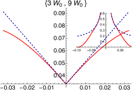
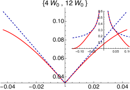
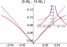
Figure 10: These figures are for the Marginal Fermi Liquid-b model Eq. (13) with parameters given in Eq. (17). The reconstructed selfenergy $\rho_{\Sigma}(\vec{k}_{F},\omega)+\frac{\eta}{\pi}$ (red curves) using the soft cutoff Eq. (9) compared with the exact value in the dashed blue curves. The two parameters relating to the soft cutoff Eq. (9) are indicated in curly brackets. The three insets show the exact spectral function in dashed blue and the cutoff included spectral function $A^{\prime}$ of Eq. (7) in the red curves. Here upper cutoff is 3 times the lower one. Here $W_{0}$ is $\sim$11 meV. Note the difference in the shape at low $\omega$ from that in Fig. (8) This version has a linear behaviour down to the lowest energy.

2.3 A Non Fermi liquid model

For the N-FL model Eq. (14), the parameters used are

$$\epsilon_{0}=1.8,\eta=0.02,\tau=0.02;\alpha_{z}=1$$ (18)

leading to a width $W_{0}=10$meV. We next display the spectral function and the real part of $G$ in Fig. (11) and the reconstructed selfenergy Fig. (12) for the N-FL model given by Eq. (14), with a few typical window parameters.

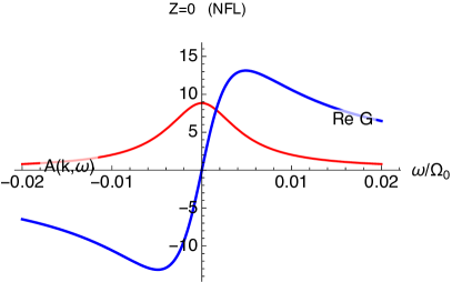
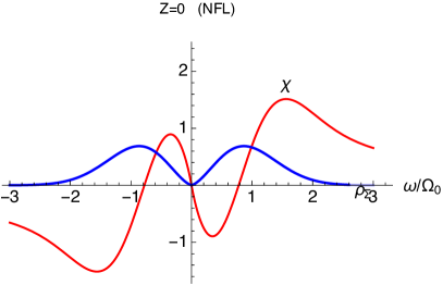
Figure 11: These figures are for the Non Fermi Liquid model Eq. (14) with parameters given in Eq. (18). (Left) The spectral function $A(\vec{k}_{F},\omega)$ and the $Re\,G(\vec{k}_{F},\omega)$ and (Right) the imaginary self energy $\rho_{\Sigma}(\vec{k}_{f},\omega)$ and $\chi(\vec{k}_{F},\omega)$, calculated from Eq. (41, 38, 48), using parameters given in Eq. (18). Here the spectral peak width $W_{0}$ is $\sim$10meV.

We now show the reconstructed selfenergy with a few typical window parameters

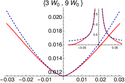
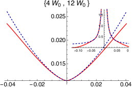
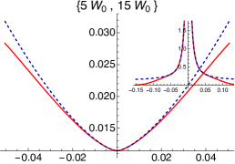
Figure 12: These figures are for the Non Fermi Liquid model Eq. (14) with parameters given in Eq. (18). The reconstructed selfenergy $\rho_{\Sigma}(\vec{k}_{F},\omega)+\frac{\eta}{\pi}$ (red curves) using the soft cutoff Eq. (9) compared with the exact value in the dashed blue curves. The two parameters relating to the soft cutoff Eq. (9) are indicated in curly brackets. The three insets show the exact spectral function in dashed blue and the cutoff included spectral function $A^{\prime}$ of Eq. (7) in the red curves. Here upper cutoff is 3 times the lower one. Here $W_{0}$ is $\sim$10 meV.

3 Comments and Conclusions

The proposal for reconstructing the selfenergy from the spectral function made in this work in Section(1.2), was illustrated above in Section(2) in a set of figures (Fig. (3)-Fig. (12)) using three typical models with different predictions. These figures show that an experimental implementation of the proposal could lead to interesting insights about the nature of quantum matter.

Different theoretical approaches to the strong correlation problem, originally inspired by the High $T_{c}$ cuprates but branching out to a much broader portfolio of materials in recent years, lead to a variety of different self energies- some of them are discussed in this work. Fundamental questions about the nature of these quantum materials remain open in most cases- it is unclear whether they constitute some variety of Fermi liquids, or some variety of non Fermi liquids. While the resistivity is often used to discriminate between these states of matter, it is a much more complex probe to interpret robustly. On the other hand a much more direct avenue to answer the above basic question, is to study the (imaginary part of the) selfenergy at low energies. At present it seems that no decisive tests using experimental ARPES data has been carried out in that direction. This is the motivation for the present paper, where we present a method to extract the low $\omega$ self energy from ARPES derived spectral function. It is based on the helpful Theorem Theorem, which assures us that the inversion method used has least error at low energies.

The proposal presented in Section(1.2) is to use Eq. (3) and a suitable windowing of the spectral function, analogous to that in Eq. (9) to infer the imaginary self energy from the ARPES derived spectral function. We provide several examples in Section(2) that show that the different model systems yield distinguishably different low energy selfenergies.

We conclude with a few comments

• The suggested inversion process can be used to estimate the elastic scattering parameter $\eta$, from the T independent part of the derived selfenergy as $\omega\to 0$.

• The observed peaks in the spectral function at $\vec{k}_{F}$ are expected to have a T dependent shift given in Eq. (LABEL:def-Deltaw, 49, 51). The shift in Eq. (51) contains the chemical potential part that can be estimated from the thermopower. The remainder has two terms in it, but is expected to be dominated by the term containing the asymmetry parameter $\alpha$ (see Eq. (11)). This can be a useful way to estimate $\alpha$ from the low energy experiments.

• The role of noise in the spectral function warrants mention; the Theorem Theorem also applies to the noise. This offers hope that at low energies, the errors due to noise are least.

• While we have focussed on $\vec{k}=\vec{k}_{F}$ here, it might be possible to explore departures from the Fermi surface if high quality spectral functions are obtainable from the intensities over a wide range of energies.

Appendix A Summary of Basic Definitions

In this section we reorganize the familiar properties of the Greens function [12, 13, 14] to define specific quantities used in our analysis.

We start with the standard expression for the retarded Greens function $G^{-1}(\vec{k},\omega_{c})={\omega_{c}}+\mu-\varepsilon_{k}-\Sigma(\vec{k},\omega_{c})$, with $\omega_{c}=\omega+i0^{+}$ [12, 13, 14]. Emphasizing the role of the spectral density of the selfenergy $\rho_{\Sigma}(\vec{k},\omega)=-\frac{1}{\pi}\mathrm{Im}\,\Sigma(\vec{k},\omega_{c})$, we decompose

$$\Sigma(k,\omega_{c}) = (1-\alpha_{z})(\omega+\mu)+\Sigma_{*}(\vec{k})-i\pi\rho_{\Sigma}(\vec{k},\omega)+\chi(\vec{k},\omega)$$

where $\chi$ can be obtained from the Hilbert transform of $\rho_{\Sigma}(\vec{k},\omega)$ as

$$\chi(\vec{k},\omega)=\mathchoice{{\vbox{\hbox{$\textstyle-$}}\kern-4.86108pt}}{{\vbox{\hbox{$\scriptstyle-$}}\kern-3.25pt}}{{\vbox{\hbox{$\scriptscriptstyle-$}}\kern-2.29166pt}}{{\vbox{\hbox{$\scriptscriptstyle-$}}\kern-1.875pt}}\!\int d\nu\frac{\rho_{\Sigma}(\vec{k},\nu)}{\omega-\nu}.$$ (20)

By definition $\lim_{\omega\to\infty}\chi(\vec{k},\omega)\to 0$ (assuming an integrable $\rho_{\Sigma}$). Here $\Sigma_{*}$ is the static part of the selfenergy, analogous to the Hartree-Fock term, which remains finite as $\omega\to\infty$. It cannot be deduced from $\rho_{\Sigma}(\vec{k},\omega)$, we see below that it can be absorbed in the measurable shifts of the peaks as defined below in Eq. (LABEL:def-Deltaw, 27). The constant $\alpha_{Z}$ is given by

$$\alpha_{z} = 1,\mbox{ Canonical (Hubbard type) Fermions}$$ (21)

$$\alpha_{z} = \frac{1}{1-\frac{1}{2}n},\mbox{ Gutzwiller projected (\ $t$-$J$ \ type) Fermions}$$ (22)

and reflects the basic nature of the Fermions in various models [15]. Using this decomposition we write

$$G^{-1}(\vec{k},\omega_{c}) = \alpha_{z}({\omega_{c}}+\mu)-\varepsilon_{\vec{k}}-\Sigma_{*}(\vec{k})-\chi(\vec{k},\omega)+i\pi\rho_{\Sigma}(\vec{k},\omega).$$

We rewrite this expression using the basic idea that at $T=0$ on the Fermi surface $G(\vec{k}_{F},\omega)$ has a pole at $\omega=0$. Since $\rho_{\Sigma}(\vec{k}_{F},0)$ vanishes,

$$\alpha_{z}\times\mu|_{T=0}=\varepsilon_{\vec{k}_{F}}+\left(\Sigma_{*}(\vec{k}_{F})+\chi(\vec{k}_{F},0)\right)|_{T=0},$$ (24)

which can be used in Eq. (LABEL:Ginv-def) to rewrite it as

$$G^{-1}(\vec{k},\omega_{c}) = {\omega_{c}}\alpha_{z}+\Delta\omega-\Delta k+\chi(\vec{k},0)-\chi(\vec{k},\omega)+i\pi\rho_{\Sigma}(\vec{k},\omega).$$

where the real functions $\Delta\omega$ the energy shift, and $\Delta k$ the momentum shift are give by

$$\Delta\omega = \alpha_{z}(\mu-\mu|_{T=0})+(\Sigma_{*}(\vec{k}_{F})|_{T=0}-\Sigma_{*}(\vec{k}_{F}))+(\chi(\vec{k}_{F},0)|_{T=0}-\chi(k_{F},0))$$

$$\Delta k = (\varepsilon_{\vec{k}}-\varepsilon_{\vec{k}_{F}})+(\Sigma_{*}(\vec{k})-\Sigma_{*}(\vec{k}_{F}))+(\chi(\vec{k},0)-\chi(\vec{k}_{F},0))$$ (27)

By their definitions, $\Delta\omega$ vanishes at T=0, while $\Delta k$ vanishes at $\vec{k}_{F}$.

At low T $\Delta\omega$ is expected to be small and may be estimated from the thermopower $S$ using the approximate Kelvin relation for thermopower $S_{Kelvin}=\frac{-1}{q_{e}}\left(\frac{\partial\mu(T)}{\partial T}\right)\Big{|}_{N,V}$, where $q_{e}$ is the electron charge.

The momentum shift $\Delta k$ (at arbitrary $T$) is of ${\cal O}(|\vec{k}-\vec{k}_{F}|)$ for $\vec{k}$ near $\vec{k}_{F}$. We now split $G(\omega+i0^{+})$ into its real and imaginary parts as

$$G(\vec{k},\omega_{c}) = \mathrm{Re}\,G(\vec{k},\omega)-i\pi A(\vec{k},\omega)$$ (28)

so that the spectral function $A(\vec{k},\omega)=-\frac{1}{\pi}\mathrm{Im}\,G(\vec{k},\omega)$. Using Eq. (LABEL:Ginv-def-2) we get

$$A(\vec{k},\omega)=\frac{\rho_{\Sigma}(\vec{k},\omega)}{\{\alpha_{z}\omega+\Delta\omega-\Delta k+\chi(\vec{k},0)-\chi(\vec{k},\omega))\}^{2}+\pi^{2}\rho^{2}_{\Sigma}(\vec{k},\omega)},$$ (29)

and

$$\mathrm{Re}\,G(\vec{k},\omega)=\frac{\{\alpha_{z}\omega+\Delta\omega-\Delta k+\chi(\vec{k},0)-\chi(\vec{k},\omega))\}}{\{\alpha_{z}\omega+\Delta\omega-\Delta k+\chi(\vec{k},0)-\chi(\vec{k},\omega))\}^{2}+\pi^{2}\rho^{2}_{\Sigma}(\vec{k},\omega)}.$$ (30)

We now recall that the real and imaginary parts of the (causal) retarded Greens function $G(\omega+i0^{+})$ are also related by the Kramers-Kronig relation

$$\mathrm{Re}\,G(\vec{k},\omega)=\mathchoice{{\vbox{\hbox{$\textstyle-$}}\kern-4.86108pt}}{{\vbox{\hbox{$\scriptstyle-$}}\kern-3.25pt}}{{\vbox{\hbox{$\scriptscriptstyle-$}}\kern-2.29166pt}}{{\vbox{\hbox{$\scriptscriptstyle-$}}\kern-1.875pt}}\!\int d\nu\frac{A(\vec{k},\nu)}{\omega-\nu},$$ (31)

so that a complete knowledge of $A$ suffices to determine $\mathrm{Re}\,G$.

Now moving in a slightly different direction, taking the imaginary part of Eq. (LABEL:Ginv-def) we get

$$\rho_{\Sigma}(\vec{k},\omega)=\frac{1}{\pi}\mathrm{Im}\,G^{-1}(\vec{k},\omega).$$ (32)

Using Eq. (28) this give $\rho_{\Sigma}$ in terms of $A(\vec{k},\omega)$ and $\mathrm{Re}G(\vec{k},\omega)$ as

$$\rho_{\Sigma}(\vec{k},\omega)=\frac{A(\vec{k},\omega)}{\{\mathrm{Re}\,G(\vec{k},\omega)\}^{2}+\{\pi A(\vec{k},\omega)\}^{2}}$$ (33)

This equation asserts that if we know the spectral function $A(\vec{k},\omega)$ for all $\omega$, we can retrieve $\rho_{\Sigma}(\vec{k},\omega)$, since the $\mathrm{Re}\,G$ can be inferred through the Hilbert transform Eq. (31). Relabeling $\mathrm{Re}\,G$ as $\Phi_{\vec{k}}(\omega)$ gives Eq. (3).

Appendix B Details of the Asymmetric Fermi Liquid Model

B.1 Scaled variables and expressions for Hilbert transforms

Let us consider a FL type model with a cubic asymmetry: We denote

$$\bar{\omega}=\frac{\omega}{\Omega_{0}},\;\;\bar{\tau}=\frac{\pi k_{B}T}{\Omega_{0}},\;\;\bar{A}=\frac{A}{\Omega_{0}},\;\;\bar{\epsilon}_{0}=\frac{\epsilon_{0}}{\Omega_{0}}$$ (34)

$$\rho_{\Sigma}(\vec{k}_{F},\omega,T) = {\epsilon_{0}}\left(\bar{\tau}^{2}+\bar{\omega}^{2}\right)\left(1-\alpha\bar{\omega}\right)e^{-\bar{\omega}^{2}}.$$ (35)

We scale the self energy with $\Omega_{0}$ so that

$$\bar{\rho}_{\Sigma}(\vec{k}_{F},\bar{\omega},\bar{\tau})={\bar{\epsilon}_{0}}\left(\bar{\tau}^{2}+\bar{\omega}^{2}\right)\left(1-\alpha\bar{\omega}\right)e^{-\bar{\omega}^{2}}$$ (36)

In this and also in other models we implicitly add an elastic scattering term $\eta/\pi$ to $\rho_{\Sigma}(\vec{k},\omega)$,

$$\rho_{\Sigma}(\vec{k},\omega)\Big{|}_{Total}=\rho_{\Sigma}(\vec{k},\omega)+\frac{\eta}{\pi},$$ (37)

as shown in Eq. (48). This term arises from impurity scattering [16], and is found to be useful in distinguishing between ARPES at different incident photon energies [18, 17]. Its corresponding real part arising from causality, is dropped since the bandwidth for this term is very large- typically a few eV’s. In practical terms adding $\eta$ is equivalent to increasing the physical temperature $T$ to $\sqrt{T^{2}+\frac{\eta}{\pi^{3}\epsilon_{0}}}$, usually this is a small effect.

In summary the model has the following parameters

• $\mbox{ strength of self energy: }\epsilon_{0}$

• $\mbox{ reduced temperature: }\bar{\tau}$

• $\mbox{ cubic asymmetry: }\alpha$

• $\mbox{ large energy scale: }\Omega_{0}$

• $\mbox{ elastic scattering scale: }\bar{\eta}$

We rewrite Eq. (36) as

$$\bar{\rho}_{\Sigma}(\vec{k}_{F},\bar{\omega},\bar{\tau}) = \bar{\epsilon}_{0}\left(\bar{\tau}^{2}\rho_{0}(\bar{\omega})+\rho_{2}(\bar{\omega})-\alpha(\bar{\tau}^{2}\rho_{1}(\bar{\omega})+\rho_{3}(\bar{\omega}))\right)$$ (38)

where

$$\rho_{m}(\bar{\omega})=e^{-\bar{\omega}^{2}}\times\bar{\omega}^{m}.$$ (39)

We write its Hilbert transform as

$$\chi(\vec{k}_{F},\omega,T) = \mathchoice{{\vbox{\hbox{$\textstyle-$}}\kern-4.86108pt}}{{\vbox{\hbox{$\scriptstyle-$}}\kern-3.25pt}}{{\vbox{\hbox{$\scriptscriptstyle-$}}\kern-2.29166pt}}{{\vbox{\hbox{$\scriptscriptstyle-$}}\kern-1.875pt}}\!\int_{-\infty}^{\infty}\frac{\rho_{\Sigma}(\vec{k}_{F},x,T)}{\omega-x}dx$$ (40)

$$= \Omega_{0}\mathchoice{{\vbox{\hbox{$\textstyle-$}}\kern-4.86108pt}}{{\vbox{\hbox{$\scriptstyle-$}}\kern-3.25pt}}{{\vbox{\hbox{$\scriptscriptstyle-$}}\kern-2.29166pt}}{{\vbox{\hbox{$\scriptscriptstyle-$}}\kern-1.875pt}}\!\int_{-\infty}^{\infty}\frac{\bar{\rho}_{\Sigma}(\vec{k}_{F},\bar{x},\bar{\tau})}{\bar{\omega}-\bar{x}}d\bar{x}.$$

By plugging in for $\rho_{\Sigma}$ we get

$$\bar{\chi}(\vec{k}_{F},\bar{\omega},\bar{\tau})\equiv\frac{1}{\Omega_{0}}\chi(\vec{k}_{F},\omega,T)=\bar{\epsilon}_{0}\left(\bar{\tau}^{2}\chi_{0}(\bar{\omega})+\chi_{2}(\bar{\omega})-\alpha(\bar{\tau}^{2}\chi_{1}(\bar{\omega})+\chi_{3}(\bar{\omega}))\right),$$ (41)

where

$$\chi_{m}(\bar{\omega}) = \mathchoice{{\vbox{\hbox{$\textstyle-$}}\kern-4.86108pt}}{{\vbox{\hbox{$\scriptstyle-$}}\kern-3.25pt}}{{\vbox{\hbox{$\scriptscriptstyle-$}}\kern-2.29166pt}}{{\vbox{\hbox{$\scriptscriptstyle-$}}\kern-1.875pt}}\!\int_{-\infty}^{\infty}\frac{\rho_{m}(\bar{x})}{\bar{\omega}-\bar{x}}d\bar{x}.$$ (42)

The evaluation of $\chi_{m}$ for even $m$ follows from the identity

$$\mathchoice{{\vbox{\hbox{$\textstyle-$}}\kern-4.86108pt}}{{\vbox{\hbox{$\scriptstyle-$}}\kern-3.25pt}}{{\vbox{\hbox{$\scriptscriptstyle-$}}\kern-2.29166pt}}{{\vbox{\hbox{$\scriptscriptstyle-$}}\kern-1.875pt}}\!\int_{-\infty}^{\infty}\frac{e^{-\alpha y^{2}}}{x-y}\,dy=2\sqrt{\pi}D_{F}(\sqrt{\alpha}x)\;\;\mbox{ with }\alpha>0,$$ (43)

by differentiating under the integral sign with respect to $\alpha$, and where $D_{F}$ is the Dawson function

$$D_{F}(x)=e^{-x^{2}}\int_{0}^{x}e^{t^{2}}\;dt.$$ (44)

For odd $m$ we use the method of partial fractions to depress the order $m$ by one, and then use the above scheme for order $m-1$. In this way we find

$$\chi_{0}(x) = \sqrt{\pi}2D_{F}(x)$$

$$\chi_{1}(x) = \sqrt{\pi}(2xD_{F}(x)-1)$$

$$\chi_{2}(x) = \sqrt{\pi}x(2xD_{F}(x)-1)$$

$$\chi_{3}(x) = \sqrt{\pi}(2x^{3}D_{F}(x)-x^{2}-\frac{1}{2}),$$ (45)

The Dawson function has a series expansion for small $x$

$$D_{F}(x)\sim x-\frac{2}{3}x^{3}+O(x^{5})$$ (46)

We read off $Z$ from this as

$$\frac{1}{Z} = \alpha_{z}-\partial_{\omega}\chi(\vec{k}_{F},\omega,T)$$ (47)

$$= \alpha_{z}-\bar{\epsilon}_{0}\left(\bar{\tau}^{2}\chi^{\prime}_{0}(\bar{\omega})+\chi^{\prime}_{2}(\bar{\omega})-\alpha(\bar{\tau}^{2}\chi^{\prime}_{1}(\bar{\omega})+\chi^{\prime}_{3}(\bar{\omega}))\right)\Big{|}_{\bar{\omega}\to 0}$$

$$= \alpha_{z}+\sqrt{\pi}\bar{\epsilon}_{0}\left(1-2\bar{\tau}^{2}\right)$$

where the prime denotes a derivative in the second line. In dimensionless (i.e. scaled) units with $\bar{\rho}_{\Sigma}=\Omega_{0}\rho_{\Sigma}$ we write

$$\bar{A}(\vec{k}_{F},\bar{\omega},\bar{\tau})=\frac{\frac{\bar{\eta}}{\pi}+\bar{\rho}_{\Sigma}(\vec{k}_{F},\bar{\omega},\bar{\tau})}{[\frac{\bar{\omega}}{Z(\bar{\omega})}-\Delta\bar{\omega}(\bar{\tau})]^{2}+[\bar{\eta}+\pi\bar{\rho}_{\Sigma}(\vec{k}_{F},\bar{\omega},\bar{\tau})]^{2}}$$ (48)

where we have added an elastic scattering constant $\bar{\eta}$ to the $\mathrm{Im}\Sigma$, and thereby a constant $\frac{\bar{\eta}}{\pi}$ to $\bar{\rho}_{\Sigma}$ here. It is important to note that the total selfenergy Eq. (37) deduced by inverting the $A$ of Eq. (48), will contain an added contribution of $\frac{\eta}{\pi}$ to $\rho_{\Sigma}$. This is commented on in the Conclusions section 3, and made specific in the captions of figures Fig. (4, 5, 6, 8, 10, 12) in the paper.

Also note that

$$\Delta\bar{\omega}(\bar{\tau})=\frac{1}{\Omega_{0}}(\mu(0)-\mu(T))+\frac{1}{\Omega_{0}}(\Sigma_{*}(\vec{k}_{F},T)-\Sigma_{*}(\vec{k}_{F},0))+\left(\bar{\chi}(\vec{k}_{F},0,\bar{\tau})-\bar{\chi}(\vec{k}_{F},0,0)\right).$$ (49)

We note the lowest order $\bar{\omega}$ expansions

$$\bar{\rho}_{\Sigma}(\vec{k}_{F},\omega) \sim \bar{\epsilon}_{0}(\bar{\omega}^{2}+\bar{\tau}^{2})(1-\alpha\bar{\omega})$$

$$\bar{\chi}(\bar{\omega},\bar{\tau}) \sim \frac{1}{2}\alpha\sqrt{\pi}\bar{\epsilon}_{0}(1+2\bar{\tau}^{2})-\sqrt{\pi}\bar{\epsilon}_{0}(1-2\bar{\tau}^{2})\bar{\omega}+{\cal O}(\bar{\omega}^{2})$$

It follows that

$$\Delta\bar{\omega}(\bar{\tau})=\frac{1}{\Omega_{0}}(\mu(0)-\mu(T))+\frac{1}{\Omega_{0}}(\Sigma_{*}(\vec{k}_{F},T)-\Sigma_{*}(\vec{k}_{F},0))+\alpha\left(\sqrt{\pi}\bar{\epsilon}_{0}\bar{\tau}^{2}\right)$$

(51)

Therefore the asymmetry parameter $\alpha$ shows up in $\Delta\bar{\omega}$ linearly. In some situations it might be reasonable to assume that this term dominates over the others, and if this is prevails then one can expect to extract $\alpha$ from the shift of the spectral peak at $\vec{k}_{F}$ as a function of $T$.

B.2 Useful properties of the peaks very close to $\omega=0$

Here we simplify the above expressions in the neighbourhood of $\omega$=0.

With

$$Z = \frac{1}{\alpha_{z}+\sqrt{\pi}\bar{\epsilon}_{0}\left(1-2\bar{\tau}^{2}\right)}$$ (52)

$$\Gamma_{0} = Z\bar{\eta}+Z\bar{\epsilon}_{0}\pi\bar{\tau}^{2}$$ (53)

$$\Gamma_{2} = Z\bar{\epsilon}_{0}\pi$$ (54)

we get

$$\bar{A}(\vec{k}_{F},\bar{\omega})\sim\frac{Z}{\pi}\frac{\Gamma_{0}+\Gamma_{2}\bar{\omega}^{2}}{(\Gamma_{0}+\Gamma_{2}\bar{\omega}^{2})^{2}+(\bar{\omega}-Z\Delta\bar{\omega})^{2}}$$ (55)

Further simplifying to a small shift $Z\Delta\bar{\omega}\ll 1$

$$\bar{A}(\vec{k}_{F},\bar{\omega})\sim\frac{Z}{\pi}\frac{\Gamma_{0}+\Gamma_{2}\bar{\omega}^{2}}{(\Gamma_{0}+\Gamma_{2}\bar{\omega}^{2})^{2}+\bar{\omega}^{2}}$$ (56)

so that $\{\bar{A}\}_{max}=\bar{A}(\vec{k}_{F},0)=\frac{Z}{\pi\Gamma_{0}}$. We note that the scaled width (FWHM) of the spectral peak used in the analysis is given by

$$\bar{W}_{0}=2\sqrt{-\frac{1}{2\Gamma_{2}^{2}}+\frac{1}{2\Gamma_{2}^{2}}\left(1+4{\Gamma_{0}^{2}\Gamma_{2}^{2}}\right)^{\frac{1}{2}}}.$$ (57)

References

- [1] X. Zhou , S. He, G. Liu, L. Zhao, Li Yu and W. Zhang, Rep. Prog. Phys. 81 062101 (2018); J. A. Sobota, Y. He, Z. X. Shen, Rev. Mod. Phys. 93, 025006 (2021).
- [2] T. Valla, A. V. Fedorov, P. D. Johnson, B.O. Wells, S. L. Hubert, Q. Li, g. D. Gu and N. Koshizuka, Science 285, 2110 (1999).
- [3] J. Jang, H. M. Yoo, L. Pfeiffer, K. West, K. W. Baldwin and R. Ashoori, Science 258, 901 (2017).
- [4] I. Vekhter and C. M. Varma, Phys. Rev. Letts. 90, 237003 (2003).
- [5] J. M. Bok, J. J. Bae, H-Y Choi, C. M. Varma, W. Zhang, J. He, Y Zhang, L. You and X. J. Zhou, Science Advances, 2, e1501329 (2016). DOI: 10.1126/sciadv.1501329.; J. H. Yun, J.M. Bok, H-Y Choi, W. Zhang, X. J. Zhou and C. M. Varma, Phys. Rev. B 84, 104521 (2011).
- [6] This relation was noted and used in B. S. Shastry, Phys. Rev. B 84, 165112 (2011) (see Eqs(22,23)), and in subsequent work of our group ([9]-b). Earlier work employing this relation could not be readily traced by the author.
- [7] The removal of the Fermi function and an instrumental resolution from the ARPES intensity is a precondition for obtaining the electron spectral function. This important problem has been extensively discussed in literature, see e.g. Refs.([1, 8]). We should note that in the present work, the focus on the spectra at at very low implies that the symmetrization of , which is sometimes regarded ([8]), ([9]-c) as being unduly biased by expectations of particle hole symmetry, may be harmless due to the smallness of the effects of asymmetry in this energy regime.
- [8] J. D. Rameau, H. B. Yang and P. D. Johnson, Journal of Electron Spectroscopy and Related Phenomena 181, 35, 2010.
- [9] (a) B. S. Shastry, Phys. Rev. Letts. 107, 056403 (2011); (b) P. Mai and B. S. Shastry, Phys. Rev. B 98, 205106 (2018); (c) B. S. Shastry, Phys. Rev. Letts. 109, 067004 (2012); (d) B S Shastry and P Mai, Phys. Rev. B101, 115121 (2020). (e) http://physics.ucsc.edu/~sriram/papers/ECFL-Reprint-Collection.pdf.
- [10] C. M. Varma, P. B. Littlewood, S. Schmitt-Rink, E. Abrahams and A. E. Ruckenstein, Phys. Rev. Letts. 63, 1999 (1989).
- [11] D. Choudhury, A. Georges, O. Parcollet and S. Sachdev, Rev. Mod. Phys. 94, 035004 (2022); S. Sachdev and J. Ye, Phys. Rev. Lett. 70 3339 (1993).
- [12] A. A. Abrikosov, L. Gorkov and I. Dzyaloshinski, Methods of Quantum Field Theory in Statistical Physics , Prentice-Hall, Englewood Cliffs, NJ (1963).
- [13] A. L. Fetter and J. D. Walecka, Quantum Theory of Many-Particle Systems, (McGraw-Hill, New York, 1971.)
- [14] P. Nozières, in Theory of Interacting Fermi Systems, (W. A. Benjamin, New York, 1964).
- [15] The constant equals unity in canonical models, but takes on a different value for Gutzwiller projected electrons. The main reason is that in the latter models, the Greens function used refers to only the lower Hubbard band states. A weight of belonging to doubly occupied states, i.e. the upper Hubbard band are thrown out. This is discussed further in B. S. Shastry and E. Perepelitsky, Phys. Rev. B 94, 045138 (2016).
- [16] E. Abrahams and C. M. Varma, Proc. Natl. Acad. Sci. USA 97, 5714(2000).
- [17] J. D. Koralek, J. F. Douglas, N. C. Plumb, Z. Sun, A. V. Fedorov, M. M. Murnane, H. C. Kapteyn, S. T. Cundiff, Y. Aiura, K. Oka, H. Eisaki, and D. S. Dessau, Phys. Rev. Lett. 96, 017005 (2006);
- [18] G. H. Gweon, B. S. Shastry and G. D. Gu, Phys. Rev. Letts. 107, 056404 (2011).