Neutron stars in the generalized SU(2) Proca theory

Abstract

The generalized SU(2) Proca theory is a vector-tensor modified gravity theory characterized by an action that remains invariant under both diffeomorphisms and global internal transformations of the SU(2) group. This study aims to further explore the physical properties of the theory within astrophysical contexts. Previous investigations have unveiled intriguing astrophysical solutions, including particle-like configurations and black holes. The purpose of this work is to constrain the theory’s free parameters by modeling realistic neutron stars. To that end, we have assumed solutions that are static, spherically symmetric, and have adopted the t’Hooft-Polyakov magnetic monopole configuration for the vector fields. Employing both analytical techniques, such as asymptotic expansions, and numerical methods involving solving boundary value problems, we have obtained neutron star solutions whose baryonic matter is described by realistic equations of state for nuclear matter. Furthermore, we have constructed mass-radius relations which reveal that neutron stars exhibit greater compactness in comparison with general relativity predictions for most of the solutions we have found and for the employed equations of state. Finally, we have found out solutions where the mass of the star is greater than $\sim$ 2.5 $M_{\odot}$; this result poses an alternative in the exploration of the mass gap of compact stellar objects.

I Introduction

In 1915, Albert Einstein published the modern vision of the gravitational interaction at the classical level: the theory of General Relativity (GR) Einstein (1915). In this theory, gravity is a manifestation of the curvature of spacetime, the latter being inextricably related to the material content of the universe. Tests of this theory, ranging from cosmological to galactic, and, specially, Solar-System scales, have been successful (see e.g. Will (2018) and references therein).

However, the standard cosmological model, also called the $\Lambda$ Cold Dark Matter model ($\Lambda$CDM), exhibits some shortcomings, particularly regarding the true nature of the exotic fluids known as dark matter and dark energy. It is worth mentioning that one of the first convincing evidences for the existence of dark matter was provided by the flatness of galactic rotation curves, see e.g. Bertone and Hooper (2018). On the other hand, type Ia supernovae have indicated that the universe is experiencing a stage of accelerated expansion today, driven by a repulsive pressure associated commonly with dark energy Amendola and Tsujikawa (2015). Modified classical gravity models, among others, constitute possible solutions to these issues (see e.g. Capozziello and De Laurentis (2011)). Moreover, besides observational concerns, GR is considered to be just an effective theory Donoghue (1994); Burgess (2004) which makes the search for models beyond Einstein’s theory a legitimate endeavour.

Among the variety of modified gravity models, we have considered in this paper the generalized SU(2) Proca theory (GSU2P) Gallego Cadavid et al. (2022a, 2020); Allys et al. (2016) (see also Gallego Cadavid et al. (2022b) for an extended version). This is a metric theory of gravity that introduces extra vector gravitational degrees of freedom and whose action is invariant under both diffeomorphisms and internal global transformations of the SU(2) group. In addition, the theory is free from the Ostrogradsky instability since it is built so that the field equations are not higher than second order. The GSU2P is closely related to its Abelian-vector and scalar counterparts, namely the Generalized Proca theory and the Horndeski theory (see e.g. Rodríguez and Navarro (2017)). Since a vector inherently induces a preferred direction, vector-tensor theories face challenges in describing the dynamics of a homogeneous and isotropic universe. One possible solution is the cosmic triad configuration (see e.g. Golovnev et al. (2008)). This configuration naturally arises within a theory exhibiting SU(2) symmetry, endowing the GSU2P with a natural framework in the cosmological scenario compared to other vector-tensor theories.

Despite the phenomenological motivations coming mainly from cosmology Rodríguez and Navarro (2017, 2018); Garnica et al. (2022), the theory must also be tested at astrophysical scales, particularly in the strong field regime where deviations from GR can manifest. A first step was taken in Martínez et al. (2023), where soliton solutions were found. In addition, Ref. Gómez and Rodríguez (2023) studied an exact black hole solution. Here, we have proceeded further and derived some consequences for relativistic stars, specifically in the context of neutron stars (NSs). These objects provide an excellent scenario to test deviations from GR. For example, constraints on the mass and radius derived from tidal deformations inferred from the gravitational wave event GW170817 Abbott et al. (2018) and data from the NICER mission Raaijmakers et al. (2019) offer valuable insights. Furthermore, the discovery of very massive NSs Demorest et al. (2010); Antoniadis et al. (2013); Romani et al. (2022) and exotic objects in the mass gap, $\sim 2.5-5\,M_{\odot}$ Ozel et al. (2010); Fishbach et al. (2020); Abbott et al. (2020); Barr et al. (2024), raises the natural question of whether these objects emerge within modified theories of gravity, such as the one studied in this paper.

The purpose of this work is twofold: first, the main one, to put constraints on the free parameters of the theory by constructing static and spherically symmetric neutron star solutions with a realistic equation of state (EOS), and, second, to provide the first hints as to whether the theory can offer possible explanations for the existence of compact objects in the mass gap.

This work is organized as follows. Section II introduces the model and presents both the equations for the structure of a neutron star in the GSU2P theory and the parameterized method for describing the realistic EOS, namely the Generalized Piecewise Polytropic fit O’Boyle et al. (2020). Section III presents analytical solutions of the field equations as asymptotic expansions near the origin and at infinity. In Section IV, the field equations are solved numerically and mass-radius equilibrium sequences are presented. Finally, Section V discusses the results and suggests directions for future work.

Throughout this article, we use geometrized units ($c=G=1$), where $c$ is the speed of light and $G$ is the universal gravitational constant. Greek indices represent spacetime indices and run from 0 to 3. Latin indices represent SU(2) group indices and run from 1 to 3. We adopt the sign convention $(+,+,+)$ according to Misner et al. (2017).

II Generalized SU(2) Proca Theory and Neutron Star solutions

The action that defines this theory was introduced originally in Allys et al. (2016) and later reconstructed in Gallego Cadavid et al. (2020) (see also Gallego Cadavid et al. (2022a)) to take into account the whole constraint algebra that avoids the propagation of unphysical degrees of freedom Errasti Díez et al. (2020a, b) (see, anyway, Janaun and Vanichchapongjaroen (2024); Errasti Díez et al. (2024)). In this paper, we have made use of the GSU2P in the form given in Garnica et al. (2022):

$$\begin{aligned} S=&\frac{1}{16\pi}\int R\ \sqrt{-g}\ d^{4}x+\frac{1}{16\pi}\int\mathcal{L}\ \sqrt{-g}\ d^{4}x\\ &+\int\mathcal{L}_{m}\ \sqrt{-g}\ d^{4}x\,,\end{aligned}$$ (1)

where $g$ is the determinant of the metric, $R$ is the Ricci scalar, $\mathcal{L}_{m}$ is a Lagrangian which depends on matter and non-gravitational fields, and

$$\begin{aligned} \mathcal{L}=-&F_{\mu\nu}^{a}F^{\mu\nu}_{a}-2\mu^{2}B^{\mu}_{a}B_{\mu}^{a}\\ &+\alpha_{1}\left(\mathcal{L}^{1}_{4,2}-2\mathcal{L}^{4}_{4,2}-\frac{20}{3}\mathcal{L}^{5}_{4,2}+5\mathcal{L}^{7}_{2}\right)\\ &+\alpha_{3}\Big{(}2\mathcal{L}^{2}_{4,2}+\mathcal{L}^{3}_{4,2}+\frac{7}{20}\mathcal{L}^{4}_{4,2}+\frac{14}{3}\mathcal{L}^{5}_{4,2}\\ &-8\mathcal{L}^{6}_{4,2}+\mathcal{L}^{7}_{2}\Big{)}\\ &+\chi_{1}\mathcal{L}^{1}_{2}+\chi_{2}\mathcal{L}^{2}_{2}+\chi_{4}\left(\mathcal{L}^{4}_{2}-\frac{\mathcal{L}^{7}_{2}}{2}\right)+\chi_{5}\mathcal{L}^{5}_{2}\\ &+\chi_{6}\left(\mathcal{L}^{6}_{2}-3\mathcal{L}^{7}_{2}\right),\end{aligned}$$ (2)

where $\mu\equiv m_{a}/\hbar$, $m_{a}$ being the mass of the vector field $B_{\mu}^{a}$ (we have chosen a common value for the three masses) and $\hbar$ being the reduced Planck constant, $F_{\mu\nu}^{a}\equiv\partial_{\mu}B_{\nu}^{a}-\partial_{\nu}B_{\mu}^{a}+\tilde{g}\epsilon^{a}_{\hskip 5.69054ptbc}B_{\mu}^{b}B_{\nu}^{c}$ is the gauge field strength tensor, with $\tilde{g}$ being the group coupling constant and $\epsilon^{a}_{\hskip 5.69054ptbc}$ being the structure constant tensor of the SU(2) group, and the $\alpha$’s and $\chi$’s are free parameters of the theory . The explicit forms of the Lagrangian pieces are given by

$$\begin{aligned} \mathcal{L}^{1}_{4,2}\equiv&\left(B_{b}\cdot B^{b}\right)\left[S^{\mu a}_{\mu}S_{\nu a}^{\nu}-S^{\mu a}_{\nu}S_{\mu a}^{\nu}\right]\\ &+2\left(B_{a}\cdot B_{b}\right)\left[S^{\mu a}_{\mu}S_{\nu}^{\nu b}-S^{\mu a}_{\nu}S_{\mu}^{\nu b}\right]\,,\end{aligned}$$ (3)

$$\begin{aligned} \mathcal{L}^{2}_{4,2}\equiv&A_{\mu\nu}^{a}S^{\mu b}_{\sigma}B^{\nu}_{a}B^{\sigma}_{b}-A_{\mu\nu}^{a}S^{\mu b}_{\sigma}B^{\nu}_{b}B^{\sigma}_{a}\\ &+A_{\mu\nu}^{a}S^{\sigma b}_{\sigma}B^{\mu}_{a}B^{\nu}_{b}\,,\end{aligned}$$ (4)

$$\begin{aligned} \mathcal{L}^{3}_{4,2}\equiv&B^{\mu a}R^{\alpha}_{\hskip 5.69054pt\sigma\rho\mu}B_{\alpha a}B^{\rho c}B^{\sigma}_{c}\\ &+\frac{3}{4}\left(B^{a}\cdot B_{a}\right)\left(B_{b}\cdot B^{b}\right)R\,,\end{aligned}$$ (5)

$$\begin{aligned} \mathcal{L}^{4}_{4,2}\equiv&\Big{[}\left(B^{a}\cdot B_{a}\right)\left(B^{b}\cdot B_{b}\right)\\ &+2\left(B^{a}\cdot B^{b}\right)\left(B_{a}\cdot B_{b}\right)\Big{]}R\,,\end{aligned}$$ (6)

$$\mathcal{L}^{5}_{4,2}\equiv G_{\mu\nu}B^{\mu a}B^{\nu}_{a}\left(B^{b}\cdot B_{b}\right)\,,$$ (7)

$$\mathcal{L}^{6}_{4,2}\equiv G_{\mu\nu}B^{\mu a}B^{\nu b}\left(B_{a}\cdot B_{b}\right)\,,$$ (8)

$$\mathcal{L}^{1}_{2}\equiv(B^{a}\cdot B_{a})(B^{b}\cdot B_{b})\,,$$ (9)

$$\mathcal{L}^{2}_{2}\equiv(B^{a}\cdot B_{b})(B^{b}\cdot B_{a})\,,$$ (10)

$$\mathcal{L}^{3}_{2}\equiv B_{\mu}^{b}B_{\rho b}A^{\mu\nu a}A^{\rho}_{\;\;\nu a}\,,$$ (11)

$$\mathcal{L}^{4}_{2}\equiv B_{\mu}^{b}B_{\rho a}A^{\mu\nu a}A^{\rho}_{\;\;\nu b}\,,$$ (12)

$$\mathcal{L}^{5}_{2}\equiv B_{\mu a}B_{\rho}^{b}A^{\mu\nu a}A^{\rho}_{\;\;\nu b}\,,$$ (13)

$$\mathcal{L}^{6}_{2}\equiv(B^{b}\cdot B_{b})A_{\mu\nu a}A^{\mu\nu a}\,,$$ (14)

$$\mathcal{L}^{7}_{2}\equiv(B^{b}\cdot B_{a})A_{\mu\nu b}A^{\mu\nu a}\,,$$ (15)

where $A^{a}_{\mu\nu}\equiv\nabla_{\mu}B_{\nu}^{a}-\nabla_{\nu}B_{\mu}^{a}$ and $S^{a}_{\mu\nu}\equiv\nabla_{\mu}B_{\nu}^{a}+\nabla_{\nu}B_{\mu}^{a}$ are, respectively, the Abelian version of the non-Abelian gauge field strength tensor and the symmetric version of $A^{a}_{\mu\nu}$, $R^{\alpha}_{\hskip 5.69054pt\sigma\rho\mu}$ is the Riemann tensor, and $G_{\mu\nu}$ is the Einstein tensor.

The explicit form given by Eq. (2) for the Lagrangian was derived to ensure that tensor perturbations on a Friedmann-Lemaître-Robertson-Walker background match those in GR at least up to second order Garnica et al. (2022). This results in luminal gravitational wave propagation and freedom from ghosts and Laplacian instabilities in the tensor sector. Compliance with the conditions imposed by the gravitational wave event GW170817 Abbott et al. (2017a) and its optical counterpart GRB 170817A Abbott et al. (2017b) supports the plausibility of the theory at cosmological scales. However, the extension of this constraint to astrophysical scales is uncertain as it depends on the specific background configuration. Determining whether luminal propagation persists near astrophysical objects requires further study, including obtaining and perturbing the background solution, which will be addressed in a future work. However, for the sake of simplicity, we have assumed that the validity of those results extends to the scale of compact objects.

II.1 Field equations

The field equations have been obtained by varying the action (1) with respect to $g^{\mu\nu}$ and $B^{a\mu}$, respectively:

$$G_{\mu\nu}=8\pi(T_{\mu\nu}^{\rm v}+T_{\mu\nu}^{m})\,,$$ (16)

$$K_{a\mu}\equiv\frac{1}{4}\frac{\delta\mathcal{L}}{\delta B^{a\mu}}=0\,,$$ (17)

where

$$T_{\mu\nu}^{\rm v}\equiv-\frac{1}{8\pi\sqrt{-g}}\frac{\delta(\mathcal{L}\sqrt{-g})}{\delta g^{\mu\nu}}\,.$$ (18)

$$T_{\mu\nu}^{m}\equiv-\frac{1}{8\pi\sqrt{-g}}\frac{\delta(\mathcal{L}_{m}\sqrt{-g})}{\delta g^{\mu\nu}}\,.$$ (19)

Appendix A in Ref. Martínez et al. (2023) contains the explicit forms of (17) and (18).

The vector fields represent additional degrees of freedom of the gravitational interaction and can be interpreted as a dark fluid. This interpretation facilitates the definition of an effective energy-momentum tensor, $T^{\rm v}_{\mu\nu}$, associated with the SU(2) vector field. However, it is worthwhile emphasising that the vector fields are fundamentally gravitational degrees of freedom. The dark fluid interpretation is merely used to compare the contributions from the vector fields with those from baryonic matter. Accordingly, we have defined the energy density and isotropic pressure associated with the vector fields, measured by an observer whose four-velocity is $u^{\mu}$, as

$$\epsilon_{\rm v}\equiv T_{\mu\nu}^{\rm v}u^{\mu}u^{\nu}\,,$$ (20)

$$P_{\rm v}\equiv\frac{1}{3}(g^{\mu\nu}+u^{\mu}u^{\nu})T_{\mu\nu}^{\rm v}\,,$$ (21)

respectively.

II.2 Static and spherically symmetric equations

We now focus on the static and spherically symmetric case in order to describe isolated and non-rotating NSs. The line element of a static and spherically symmetric spacetime in Schwarzschild coordinates is given by

$$ds^{2}=-e^{2\Phi(r)}dt^{2}+h(r)^{-1}dr^{2}+r^{2}(d\theta^{2}+\sin^{2}\theta d\phi^{2})\,,$$ (22)

where $h(r)\equiv 1-2m(r)/r$. Given the structure of the field equations, we have found it more convenient to use the variable $e^{-2\delta}\equiv e^{2\Phi}/h$.

The configuration we have chosen for the vector field $B_{\mu}^{a}$ is given by the t’Hooft-Polyakov monopole ansatz which is a special case of the more general spherically symmetric one Witten (1977) (see also Refs. Sivers (1986); Forgacs and Manton (1980)):

$$\mathbf{B}=-\frac{\tau^{a}}{\tilde{g}}\biggl{[}\epsilon_{ajk}x^{k}\frac{(1+w)}{r^{2}}dx^{j}\biggr{]}\,,$$ (23)

where $\tau^{a}=-i\sigma^{a}/2$ is a basis for the SU(2) algebra with $\sigma^{a}$ being the Pauli matrices, $x^{a}$ (or $x^{j}$) are the space-time cartesian coordinates, and $\epsilon_{aij}$ is the Levi-Civita tensor. The cartesian coordinates $x^{i}$ can be obtained from the polar spherical coordinates $(r,\theta,\phi)$ in the same way as in flat space Bartnik and McKinnon (1988); Greene et al. (1993). Thus, the t’Hooft-Polyakov monopole has the following more convenient form:

$$\mathbf{B}=(1+w)(\tau_{\theta}\sin\theta d\phi-\tau_{\phi}d\theta)\,,$$ (24)

where

$$\tau_{r} =\sin\theta\cos\phi\,\tau_{1}+\sin\theta\sin\phi\,\tau_{2}+\cos\theta\,\tau_{3}\,,$$ (25)

$$\tau_{\theta} =\cos\theta\cos\phi\,\tau_{1}+\cos\theta\sin\phi\,\tau_{2}-\sin\theta\,\tau_{3}\,,$$ (26)

$$\tau_{\phi} =-\sin\phi\,\tau_{1}+\cos\phi\,\tau_{2}\,,$$ (27)

is a polar spherical basis for the SU(2) algebra.

For the NS, we have considered a single perfect fluid, $(T^{m})^{\mu}{}_{\nu}={\rm diag}(-\epsilon(r),P(r),P(r),P(r))$, where $\epsilon$ and $P$ are the energy density and pressure, respectively, measured by a static observer with respect to the fluid. The rest mass density of baryonic matter is denoted by $\rho$. The equation of motion for matter is given by the continuity equation, $\nabla_{\nu}T_{m}^{\mu\nu}=0$, which reduces to

$$P^{\prime}=-(P+\epsilon)\Phi^{\prime}=(P+\epsilon)\biggl{(}\frac{m-rm^{\prime}}{2mr-r^{2}}+\delta^{\prime}\biggr{)}\,,$$ (28)

where the prime means a derivative with respect to $r$.

The equations in the static and spherically symmetric case, together with the t’Hoof-Polyakov ansatz, have a rather complicated form which can be found in Appendix A.

In order to obtain objects that correspond to isolated solutions, the asymptotically flatness condition must be satisfied. Thus, we have imposed boundary conditions at spatial infinity $r\to\infty$ so that $\Phi\to 0,\delta\to 0$, and $m\to{\rm const.}$ The radius of the NS is obtained by requesting the condition

$$P(R)=0\,,$$ (29)

and by requiring that both the pressure and the energy density of the baryonic matter vanish when $r>R$. This does not imply by any means, however, that the vector fields outside the NS get a trivial value. The Arnowitt-Deser-Misner (ADM) mass $M$, which in this static and spherically symmetric case coincides with the Komar mass Wald (2010), is given by the asymtoptic value of the mass function

$$M=\lim_{r\to\infty}m(r)=\lim_{r\to\infty}\frac{r}{2}(1-h)\,.$$ (30)

Besides, following Bartnik and McKinnon (1988), we have defined an effective charge,

$$Q_{\rm eff}^{2}\equiv 2r(M-m)\,.$$ (31)

This charge does not represent the strength of an interaction, it is only used to quantify the departure of the metric solution from the Schwarzschild one.

Finally, the group coupling constant $\tilde{g}$ has inverse units of length in geometrized units. Accordingly, we have defined the normalized variables $\hat{r}\equiv r\tilde{g}$, $\hat{m}\equiv m\tilde{g}$, $\hat{P}\equiv P\tilde{g}^{-2}$ and $\hat{\epsilon}=\epsilon\tilde{g}^{-2}$. Since we are interested in astrophysical scales, we set the unit length to $\tilde{g}^{-1}=M_{\odot}=1.477$ km.

II.3 Equations of state for the NS

For this paper, we have explored baryonic matter EOSs that are able to model objects with more than $2\leavevmode\nobreak\ M_{\odot}$ in GR and agree with the data from NICER Riley et al. (2019, 2021). Thus, in this context, we have allowed for the possibility of having more massive configurations within this theory. Among the NS EOSs in the literature, we have chosen to work with the H4 Lackey et al. (2006) and the GM1Y6 Glendenning and Moszkowski (1991); Oertel et al. (2015) EOSs. Both EOSs correspond to matter formed by electrons, nucleons, and hyperons.

For simplicity in our numerical calculations, these EOSs are parameterized using the Generalized Piecewise Polytropic fit O’Boyle et al. (2020). We divide the baryonic rest mass density range in $N$ intervals. Within each interval, spanning from $\rho_{i}$ to $\rho_{i+1}$, the pressure and energy density are:

$$P(\rho) = K_{i}\rho^{\Gamma_{i}}+\Lambda_{i}\,,$$ (32)

$$\epsilon(\rho) = \frac{K_{i}}{\Gamma_{i}-1}\rho^{\Gamma_{i}}+(1+a_{i})\rho-\Lambda_{i}\,.$$ (33)

The polytropic indices, $\Gamma_{i}$, and the dividing densities, $\rho_{i}$, are the fit parameters of the method. For the high-density region of the EOSs (densities greater than the nuclear saturation density, $\rho_{s}\approx 2.4\times 10^{14}$ g cm^-3), we have used a three-zone Piecewise Polytropic model (see Table 1) (see Becerra et al., 2024, for more details), while for the low-density region ($\rho<\rho_{s}$), we have employed the five zone parametrization presented in O’Boyle et al. (2020).

The values of the constants $K_{i}$, $\Lambda_{i}$ and $a_{i}$ are established by ensuring the continuity of the energy density, pressure and sound speed at the dividing densities:

$$K_{i+1} = K_{i}\frac{\Gamma_{i}}{\Gamma_{i+1}}\rho^{\Gamma_{i}-\Gamma_{i+1}}\,,$$ (34)

$$\Lambda_{i+1} = \Lambda_{i}+\left(1-\frac{\Gamma_{i}}{\Gamma_{i+1}}\right)K_{i}\rho^{\Gamma_{i}}\,,$$ (35)

$$a_{i+1} = a_{i}+\Gamma_{i}\frac{\Gamma_{i+1}-\Gamma_{i}}{(\Gamma_{i+1}-1)(\Gamma_{i}-1)}K_{i}\rho^{\Gamma_{i}-1}\,.$$ (36)

The above recurrence relations are solved by setting the parameters in the lowest density zone to $a_{8}=0$, $\Lambda_{8}=0$ and $K_{8}=5.21\times 10^{-9}c^{2}$ in cgs units, where $c$ is the speed of light.

EOS	$\mathbf{\log\rho_{1}}$	$\mathbf{\log\rho_{2}}$	$\mathbf{\log\rho_{3}}$	$\Gamma_{1}$	$\Gamma_{2}$	$\Gamma_{3}$
	$[\mathrm{g\,cm^{-3}}]$	$[\mathrm{g\,cm^{-3}}]$	$[\mathrm{g\,cm^{-3}}]$
H4	$14.99$	$14.87$	$13.49$	$2.51$	$2.33$	$1.56$
GM1Y6	$14.99$	$14.87$	$13.75$	$2.96$	$1.62$	$1.63$

Table 1: High-density Generalized Piecewise Polytropic fit parameters for the H4 and GM1Y6 EOSs.

III Asymptotic series solution at the origin and at spatial infinity

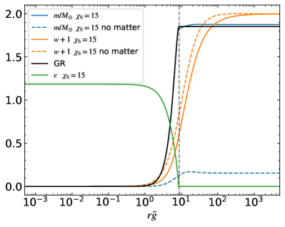
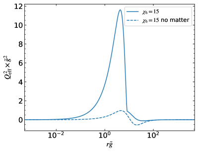
Figure 1: Left: example of a 1-node solution in the minimal coupling case $\chi_{6}=15$. We have used here the EOS H4 and central rest-mass density $\rho_{0}=1\times 10^{15}$ g cm^-3. The mass function $m$ is shown in blue (continuous line) and the vector field $w$ in orange (continuous line). The NS solution in GR is shown as a continuous black curve. The GSU2P solution departs from the GR mass function at a radius $r\tilde{g}\sim 1$ where the vector field starts to increase. For comparison and contrast, we also show the particle-like (no baryonic matter) solution, with dashed lines, employing the chosen value for $\chi_{6}$. For the case $\chi_{6}=15$, the energy density of baryonic matter is shown in green and the radius of the NS as the vertical dashed grey line. Right: effective charge (31) for the GSU2P solutions shown in the left panel.

In order to find a regular solution at the origin, we have expanded the field variables as asymptotic power series:

$$\hat{m} =a_{3}\hat{r}^{3}+a_{5}\hat{r}^{5}+\mathcal{O}(\hat{r}^{6})\,,$$ (37)

$$w =-1+b_{2}\hat{r}^{2}+b_{4}\hat{r}^{4}+\mathcal{O}(\hat{r}^{6})\,,$$ (38)

$$\Phi =1+c_{2}\hat{r}^{2}+c_{4}\hat{r}^{4}+\mathcal{O}(\hat{r}^{6})\,,$$ (39)

$$\hat{P} =\hat{P}_{0}+d_{2}\hat{r}^{2}+d_{4}\hat{r}^{4}+\mathcal{O}(\hat{r}^{6})\,,$$ (40)

where $\hat{P}_{0}$ is the normalized central pressure of the baryonic matter. The different coefficients have been found by solving the equations of structure (46)-(51). The explicit value of the non-vanishing coefficients can be found in the Appendix B. The series depend on both $b_{2}$ and on the value of the pressure of the baryonic matter at the centre.

The coefficient $b_{2}$ is arbitrary and is related to the central normalized energy density associated to the vector fields, $2\pi\hat{\epsilon}_{\rm v}(0)=3b_{2}^{2}$. The coefficient $d_{1}$ vanishes and $d_{2}<0$, thus the pressure reaches a (local) maximum at the origin, as expected. The leading contributions in the series come from the baryonic matter and from the Einstein-Yang-Mills (EYM) theory. Modifications in the behaviour of the field variables are expected to appear in the intermediate region $\hat{r}\sim 1$ where the vector fields are not trivial. The pressure and density of the baryonic matter is also seen to be modified explicitly at higher orders by the vector fields which shows that the new gravitational degrees of freedom indeed alter the baryonic matter distribution in the star.

There is no an equivalent to the Birkhoff’s theorem in the GSU2P theory. Consequently, we must search for the possible vacuum asymptotically flat solutions. In order to achieve this task, we have expanded the variables at spatial infinity as symptotic series in inverse powers of $r$:

$$\hat{m} =\hat{M}+\frac{\tilde{a}_{1}}{\tilde{r}}+\frac{\tilde{a}_{2}}{\hat{r}^{2}}+\frac{\tilde{a}_{3}}{\hat{r}^{3}}+\mathcal{O}\left(\frac{1}{\hat{r}^{4}}\right)\,,$$ (41)

$$w =w_{\infty}+\frac{\tilde{b}_{1}}{\hat{r}}+\frac{\tilde{b}_{2}}{\hat{r}^{2}}+\frac{\tilde{b}_{3}}{\hat{r}^{3}}+\mathcal{O}\left(\frac{1}{\hat{r}^{4}}\right)\,,$$ (42)

$$\Phi =\Phi_{\infty}+\frac{\tilde{c}_{1}}{\hat{r}}+\frac{\tilde{c}_{2}}{\hat{r}^{2}}+\frac{\tilde{c}_{3}}{\hat{r}^{3}}+\mathcal{O}\left(\frac{1}{\hat{r}^{4}}\right)\,,$$ (43)

and have solved the field equations. The solutions have the same form as in the particle-like case (see Martínez et al. (2023) for details) with the same free parameters (which are determined later by numerical integration). Therefore, there exist asymptotically flat solutions as required. It remains to answer the question whether these solutions can be matched with the solutions found near the origin. For this task, we have proceeded to numerically solve the equations of structure by a shooting method with parameter $b_{2}$. The two asymptotic solution are matched in an intermediate region numerically and the free parameters of both asymptotic series are determined.

Particle-like solutions and NS solutions share the same form of the asymptotic series at infinity but the free coefficients are different, e.g. the ADM mass is different. This comes from the fact that the behaviour of the field variables is different in the intermediate region due to the presence of baryonic matter (see Fig. 1).

IV 1-node neutron stars solutions

We have solved the structure equations using a shooting method with the parameter $b_{2}$ to match the asymptotic solution at infinity. Given the complexity of the GSU2P theory, we have selected two representative cases in the Lagrangian. One case involves the vector fields being minimally coupled to the metric where $\chi_{6}\neq 0$ and all other parameters vanish. The other case involves a non-minimal coupling where $\alpha_{1}\neq 0$ and all other parameters vanish. The different solutions can be classified by the number of nodes in the field variable $w$. We have focused on the 1-node solutions since they are potentially stable in the particle-like case Martínez et al. (2023).

Before starting the numerical integration of the structure equations in the GSU2P theory, we conducted exploratory work in the standard EYM case which, to the best of our knowledge, had not been studied so far. Interestingly, we have found solutions in the presence of baryonic matter. However, these solutions turned out to be unrealistic, consisting of a very small core of baryonic matter surrounded by an extended halo made of YM fields. These objects resemble the EYM soliton with a very compact baryonic mass core. For these objects, the energy density of the (gravitational) vector fields is dominant over the non-gravitational fields. This phenomenon was also observed at cosmological scales, as shown in García-Serna et al. (2024). Therefore, to construct realistic NS models, we searched for cases within the GSU2P theory where the YM energy was screened by the other Lagrangian terms. Based on the above discussion, we have not reported solutions in the EYM case here because they are not of astrophysical interest.

IV.1 Minimal coupling case

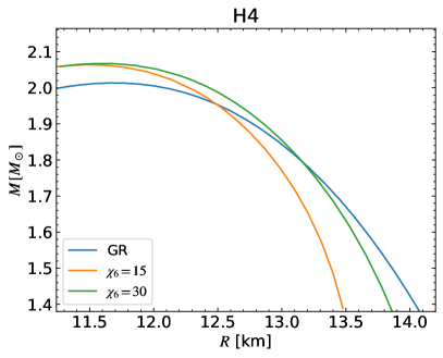
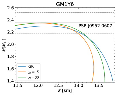
Figure 2: ADM mass versus radius of a NS whose baryonic matter is described by the EOS H4 (left) and GM1Y6 (right) for the minimal case $\chi_{6}$. The horizontal line corresponds to the mass of the potentially heaviest observed NS PSR J0952-0607 ($2.35\pm 0.17M_{\odot}$), and the $1\sigma$ uncertainty Romani et al. (2022) (dashed horizontal lines).

We have aimed at identifying cases where the YM energy is at least comparable to the central energy density of baryonic matter. To achieve this, as a first approximation, we have used an EOS described by a single polytropic equation. For the minimal coupling case, we have found that $\chi_{6}\gtrsim 10$ fulfils this requirement.

Next, we have employed a realistic EOS with the parameterization described in Subsection II.3. In Fig. 1, we show the behaviour of the mass function $m$ and the vector field $w$ for the specific case $\chi_{6}=15$ with EOS H4 and central rest-mass density $\rho_{0}=1\times 10^{15}$ g cm^-3. The mass function is seen to deviate from the GR case from the intermediate region $r\tilde{g}\approx 1$ where the vector field value is non-trivial, $w\neq\pm 1$. The mass function continues to increase even though the energy density of baryonic matter has vanished, see the green curve in the left panel of Fig. 1. This occurs because the energy density of the vector fields does not vanish at the same radius as the baryonic matter does; instead, it decreases more slowly outside the star, keeping its contribution to the gravitational mass.

In Fig. 1, we have also compared the NS solution and the one with no baryonic matter, i.e., the particle-like solution using the same value for $\chi_{6}$ for comparison. The mass of the particle-like solution is seen to be much less than that of the NS in both the GSU2P theory and GR. Nevertheless, the mass of the NS in the GSU2P is greater than in GR because of the contribution of the vector fields, although this is not a linear effect as can be appreciated in the left panel of the same figure. In addition, the presence of baryons increases notably the value of the effective charge, see (31) and the right panel of Fig. 1.

In Fig. 2, we show the equilibrium sequence of mass versus radius for two different values of the parameter $\chi_{6}$, and for the EOS H4 (left panel) and EOS GM1Y6 (right panel). The maximum mass is greater than in the GR case. When the central density of the baryonic mass decreases, the contribution of the vector fields increases and the radius becomes smaller. As a consequence, as the ADM mass decreases, the radius becomes smaller, and there is a tendency to create a very compact core of baryonic matter as in the EYM case.

In the GR case, the selected EOSs exhibit a maximum mass that is less than the central value of the mass of the observed pulsar PSR J0952-0607, but within $1\sigma$ uncertainty. In the GSU2P case, the maximum mass is closer to this central value of the heaviest observed NS.

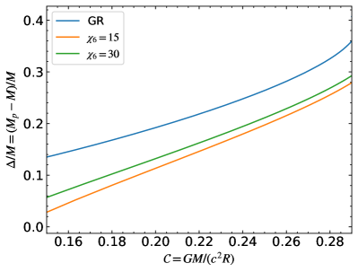
Figure 3: Specific gravitational binding energy $\Delta/M=(M_{p}-M)/M$ for the equilibrium sequence shown in the right panel of Fig. 2.

In order to assess the stability of the star, we have computed the proper mass-energy

$$M_{p}=\int_{0}^{r_{s}}\frac{4\pi r^{2}\epsilon}{\sqrt{1-2m(r)/r}}dr\,,$$ (45)

and the gravitational binding energy, $\Delta\equiv M_{p}-M$ Cameron (1959). We have found that this last value is generally positive, see Fig. 3, satisfying the minimum necessary condition for stability. Nevertheless, to properly check the stability, the explicit perturbation theory must be carried out which will be left for a future work. When the effective energy density associated to the vector fields (tends to) become(s) dominant, $\Delta$ tends to become negative, i.e., when the energy density is dominated by the vector fields, especially by the YM term, the configuration can be unstable as expected from the particle-like EYM solutions.

Finally, for this minimally coupled case, we have explored evidence suggesting the possible existence of objects within the mass gap of $2.5\,M_{\odot}<M<5\,M_{\odot}$. We have specifically searched for NS solutions with masses greater than those we have found previously, while maintaining a similar level of compactness. To achieve this and only here, we have adjusted the value of the gauge coupling constant. As previously mentioned, the gauge coupling constant represents the mass-length scale of the system. Altering the value of $\tilde{g}$ changes the mass and length of the configurations. However, this change is not merely a rescaling factor due to the presence of baryonic matter. For particle-like solutions, modifying the group constant does result in a rescaling of the solutions.

We have found NS solutions with $\tilde{g}$ slightly less than $M_{\odot}^{-1}$ which are more massive than the previous NS solutions. The mass-radius equilibrium sequences with $\chi_{6}=15$, for the EOS GM1Y6 and two additional values of $\tilde{g}$, are shown in Fig. 4.

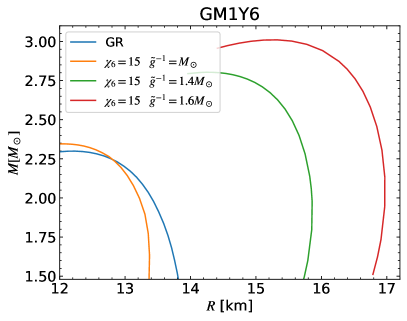
Figure 4: ADM mass versus radius of a NS whose baryonic matter is described by the EOS GM1Y6. We have fixed, in this case, the parameter $\chi_{6}=15$ for the minimal coupling scenario and varied the group coupling constant $\tilde{g}$ as indicated.

IV.2 Non-minimal coupling case

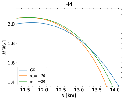
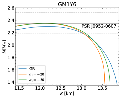
Figure 5: ADM mass versus radius of a NS whose baryonic matter is described by the EOS H4 (left) and GM1Y6 (right) for the non-minimal coupling case $\alpha_{1}$. The horizontal line corresponds to the mass of the potentially heaviest observed NS PSR J0952-0607 ($2.35\pm 0.17M_{\odot}$), and the $1\sigma$ uncertainty Romani et al. (2022) (dashed horizontal lines).

We continue with the non-minimal coupling case, $\alpha_{1}\neq 0$ and all other parameters vanishing. We have proceeded in a similar way to the minimal coupling case by first using a single polytropic EOS to determine the range for the parameter $\alpha_{1}$ so that the energy density of the vector fields does not dominate over the baryonic matter. We have found that to fulfill this requirement, $\alpha_{1}\lesssim-10$.

We have constructed equilibrium sequences of mass versus radius for the selected EOS which are shown in Fig. 5. The behaviour is similar to the minimal coupling case. The maximum mass is greater than in GR and the NSs are more compact than in GR as well. However, the NSs are less compact than in the minimal coupling case. Again, the excess in gravitational mass comes from the contribution of the vector fields.

As mentioned before, the YM energy is dominant and creates very compact cores of baryonic matter. To construct a realistic NS model, there must be a counterterm in the full Lagrangian to cancel out the contribution of the YM term. The piece of the Lagrangian associated with $\alpha_{1}$ involves more terms and we have found in our solutions that its screening effect is greater than that of the simpler piece $\chi_{6}$.

The behaviour of the central energy density associated with the vector fields is shown in Fig. 6. For both EOSs, when the baryonic matter decreases, the shooting parameter is seen to grow and the contribution to the gravitational mass from the vector fields becomes more significant. We have also found that, in general, the binding energy is positive, thus the configurations are potentially stable.

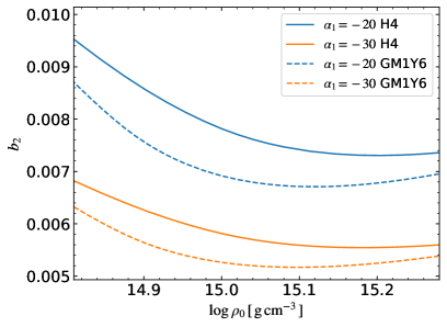
Figure 6: Shooting parameter (central energy density associated with the vector fields) versus central density of baryonic matter for different values of the coupling parameter and both EOSs as indicated in the legend.

V Conclusions

Ongoing efforts to describe compact objects in alternative theories of gravity have consolidated a promising programme to test gravity in the strong-field regime. Under this premise, we have examined in this work the effects of additional gravitational degrees of freedom on the baryonic matter of NSs within the GSU2P theory. We have employed both analytical and numerical methods to solve the equations of structure for static and spherically symmetric NSs, with realistic EOSs, namely H4 and GM1Y6. Although our results marginally depend on the EOS, which distinguishes high-density and low-density regions, they provide a preliminary but compelling approach to model realistic NSs in this alternative gravity theory.

Within the framework of the EYM theory in the presence of baryonic matter, we initially observed that this type of solution exhibits a small core surrounded by a halo composed of vector fields. This result raises the question of whether a similar object is formed in the GSU2P theory or whether a more extended baryonic dense core can be formed instead. To elucidate this behaviour, we have analyzed two cases within the GSU2P theory: one featuring minimal coupling between the metric tensor and the vector fields, and the other with non-minimal coupling. For the purposes of this work, the additional vector gravitational degrees of freedom, i.e., those described by $B^{a}_{\mu}$, have been treated as a dark fluid.

As a general trend, we have observed that the YM term tends to dominate the energy content when the free parameters are very small, approaching zero. This suggests a detailed exploration of the parameter space of the theory, for the cases where the dark fluid dominates the energy content. As a matter of fact, we have explored the parameter space of $\chi_{6}$ and $\alpha_{1}$ to ensure that the YM energy density does not dominate over the contribution associated with baryonic matter. Specifically, we have determined the ranges $\chi_{6}\gtrsim 10$ and $\alpha_{1}\lesssim-10$, within which the YM contribution remains subdominant. This allows for the formation of realistic NSs with a non-trivial vector field configuration surrounding the baryonic core.

As a main conclusion of this work, we have found that NSs within the GSU2P theory exhibit greater compactness compared to those in GR with the same central baryonic mass density. This effect is due to the energy contribution of the vector fields to the gravitational mass, which can be interpreted as the possible repulsive behaviour of the vector fields just as was shown in Martínez et al. (2023). The first astrophysical implication of this result is the suitable explanation for very heavy NSs such as PSR J0952-0607. All these quantitative features can be described in both the minimal and non-minimal coupling cases. Moreover, these solutions enjoy the good property of stability, although based on the criteria of the binding energy which is a necessary but not a sufficient condition. This encourages employing more sophisticated methods based on perturbative arguments. This is a crucial aspect we are planning on addressing in a future work. It is worthwhile mentioning that GR is consistent to $1\sigma$ with the mass of PSR J0952-0607.

The next question we have addressed in this work is whether the theory can account for the mass gap. Interestingly, by properly fixing the group coupling constant $\tilde{g}$, the solution can be straightforwardly accommodated in the mass gap, providing a satisfactory explanation for the existence of massive compact objects beyond GR expectations. But, do these objects truly offer a purely gravitational explanation for the mass gap? Although this is a first step towards addressing this issue, it is necessary to explore the parameter space of the theory more comprehensively, along with a more rigorous treatment of stability. This will allow us to arrive at a more conclusive answer. On the other hand, whether there is a mass gap or not in the heart of GR is a subject that can shed light on the physics of supernova explosions, mass accretion of neutron stars, binary mergers, and potentially on the gravitational theory that governs these phenomena. Finally, the pressure of the vector fields in the t’Hooft-Polyakov configuration is anisotropic, so it may be interesting to analyze compact stars with an anisotropic EOS.

With the aid of current and future high-precision data, we aim at testing the consistency of this theory in other astrophysical scenarios and further constrain the untested parts of the theory. For example, gravitational wave observations from various astrophysical events can provide insights into any deviation from GR waveforms Yunes and Siemens (2013); Perkins et al. (2021); Moore et al. (2021). In addition, pulsar timing can reveal deviations in the timing residuals caused by the presence of fundamental (vector) fields Afzal et al. (2023); Zhang et al. (2023). These examples, though speculative, offer stringent tests that may reveal the presence of fundamental massive vector fields around strong gravitational backgrounds in the form proposed in this paper.

Appendix A Equations of structure

This appendix shows the explicit form of the equations of structure. When there is only a minimal coupling between the spacetime geometric structure and the vector fields, i.e. for $\alpha_{1}=\alpha_{3}=0$ in (2), the equations are:

$$m^{\prime}+\frac{(2m-r)w^{\prime 2}\left[\tilde{g}^{2}r^{2}+(w+1)^{2}\chi_{56}\right]}{\tilde{g}^{4}r^{3}}+\frac{4\chi_{6}(w+1)^{4}}{\tilde{g}^{4}r^{4}}\\ +\frac{(w+1)^{2}\left[(w+1)^{2}\chi_{12}-\tilde{g}^{2}(w-1)^{2}-2\mu^{2}\tilde{g}^{2}r^{2}\right]}{2\tilde{g}^{4}r^{2}}=4\pi r^{2}\epsilon\,,$$ (46)

$$\delta^{\prime}+\frac{2w^{\prime 2}\left[\tilde{g}^{2}r^{2}+(w+1)^{2}\chi_{56})\right]}{\tilde{g}^{4}r^{3}}+\frac{4\pi r^{2}(P+\epsilon)}{r-2m}=0\,,$$ (47)

$$r(r-2m)\left[(w+1)^{2}\chi_{56}+\tilde{g}^{2}r^{2}\right]w^{\prime\prime}+r\chi_{56}(w+1)(r-2m)w^{\prime 2}-2r\left[\tilde{g}^{2}r^{2}+(w+1)^{2}\chi_{56}\right]m^{\prime}w^{\prime}\\ -r(r-2m)\left[\tilde{g}^{2}r^{2}+(w+1)^{2}\chi_{56}\right]w^{\prime}\delta^{\prime}+\left[2m\tilde{g}^{2}r^{2}+2(w+1)^{2}\chi_{56}(3m-r)\right]w^{\prime}\\ +r^{2}(w+1)\left[\tilde{g}^{2}(w-\mu^{2}r^{2}-w^{2})+(w+1)^{2}\chi_{12}\right]+8\chi_{6}(w+1)^{3}=0\,,$$ (48)

where $\chi_{12}\equiv 2\chi_{1}+\chi_{2}$ and $\chi_{56}\equiv\chi_{6}-\chi_{5}$. As already mentioned in Martínez et al. (2023), the parameter $\chi_{4}$ has no contribution to the field equations.

Now, for the case $\chi_{1}=\chi_{2}=\chi_{4}=\chi_{5}=\chi_{6}=0$ in (2) the respective equations are:

$$\left\{1+\mathcal{C}_{1}\left[\frac{(w+1)}{\tilde{g}^{2}r}-2\frac{w^{\prime}}{\tilde{g}^{2}}\right]\right\}m^{\prime}-\frac{h}{\tilde{g}^{2}}\left(1-\mathcal{C}_{2}\right)w^{\prime 2}-2\left[h\,\mathcal{C}_{3}-\mathcal{C}_{1}\frac{m}{r}\right]\frac{w^{\prime}}{\tilde{g}^{2}}\\ +\frac{2rh\,\mathcal{C}_{1}}{\tilde{g}^{2}}w^{\prime\prime}-\frac{\mu^{2}(w+1)^{2}}{\tilde{g}^{2}}-\frac{\left(w^{2}-1\right)^{2}}{2\tilde{g}^{2}r^{2}}+\frac{4\left(25\alpha_{1}-36\alpha_{3}\right)(w+1)^{4}}{5\tilde{g}^{4}r^{4}}\\ -\frac{\left(880\alpha_{1}-1003\alpha_{3}\right)m(w+1)^{4}}{15\tilde{g}^{5}r^{5}}=4\pi r^{2}\epsilon\,,$$ (49)

$$h\,\left[1+\frac{\mathcal{C}_{1}(1+w)}{r}\right]\frac{\Phi^{\prime}}{\tilde{g}^{2}}-h\,\left(1-\mathcal{C}_{4}\right)\frac{w^{\prime 2}}{\tilde{g}^{2}r}-\frac{2h\,\mathcal{C}_{1}}{\tilde{g}^{2}}\Phi^{\prime}w^{\prime}-2h\mathcal{C}_{5}\frac{w^{\prime}}{\tilde{g}^{2}}-\frac{m}{r^{2}}+\frac{\left(w^{2}-1\right)^{2}}{2\tilde{g}^{2}r^{3}}\\ +\frac{\mu^{2}(w+1)^{2}}{\tilde{g}^{2}r}+\frac{\left(140\alpha_{1}-101\alpha_{3}\right)(w+1)^{4}}{5\tilde{g}^{4}r^{5}}-\frac{2\left(100\alpha_{1}-89\alpha_{3}\right)m(w+1)^{4}}{5\tilde{g}^{4}r^{6}}=4\pi rP\,,$$ (50)

$$rh\,\mathcal{C}_{1}\left(\Phi^{\prime\prime}+\Phi^{\prime 2}\right)-\mathcal{C}_{1}\Phi^{\prime}m^{\prime}+h\left(1-\mathcal{C}_{4}\right)\Phi^{\prime}w^{\prime}+h\left(r\mathcal{C}_{5}+\mathcal{C}_{1}\frac{m}{r}\right)\Phi^{\prime}-\mathcal{C}_{5}m^{\prime}\\ +\left(\frac{\mathcal{C}_{4}-1}{r}\right)m^{\prime}w^{\prime}+h\,(1-\mathcal{C}_{4})w^{\prime\prime}-h\,\mathcal{C}_{4}w^{\prime 2}+\left[2h\,\mathcal{C}_{4}+\frac{m}{r}\left(1-\mathcal{C}_{4}\right)\right]\frac{w^{\prime}}{r}\\ -\mu^{2}(w+1)-\frac{w\left(w^{2}-1\right)}{r^{2}}-\frac{\left(8\alpha_{1}+3\alpha_{3}\right)(w+1)^{3}}{\tilde{g}^{2}r^{4}}-\frac{\left(16\alpha_{1}-19\alpha_{3}\right)m(w+1)^{3}}{3\tilde{g}^{2}r^{5}}=0\,,$$ (51)

where

$$\mathcal{C}_{1} \equiv\frac{\left(40\alpha_{1}-67\alpha_{3}\right)(w+1)^{3}}{15\tilde{g}^{2}r^{3}}\,,$$ (52)

$$\mathcal{C}_{2} \equiv\frac{\left(85\alpha_{1}-124\alpha_{3}\right)(w+1)^{2}}{5\tilde{g}r^{2}}\,,$$ (53)

$$\mathcal{C}_{3} \equiv\frac{\left(320\alpha_{1}-407\alpha_{3}\right)(w+1)^{3}}{15\tilde{g}^{2}r^{3}}\,,$$ (54)

$$\mathcal{C}_{4} \equiv\frac{\left(\alpha_{1}+2\alpha_{3}\right)(w+1)^{2}}{\tilde{g}^{2}r^{2}}\,,$$ (55)

$$\mathcal{C}_{5} \equiv\frac{\left(160\alpha_{1}-139\alpha_{3}\right)(w+1)^{3}}{15\tilde{g}^{2}r^{4}}\,.$$ (56)

Appendix B Coefficients of the asymptotic series near the origin

This appendix presents the values of the non-vanishing coefficients of the asymptotic series near the origin (37)-(40), obtained by solving the equations of structure shown in the previous appendix:

$$a_{3}=\frac{4\pi\hat{\epsilon}_{0}}{3}+2b_{2}^{2}\,,$$ (57)

$$a_{5}=-\frac{8}{15}\pi^{2}\Xi\left(\hat{P}_{0}+\hat{\epsilon}_{0}\right)\left(3\hat{P}_{0}+\hat{\epsilon}_{0}\right)\\ -\frac{8}{15}\pi\left[(3\Xi-2)\hat{\epsilon}_{0}+3(\Xi+2)\hat{P}_{0}\right]b_{2}^{2}+\frac{3\mu^{2}}{5}b_{2}^{2}\\ -\frac{8b_{2}^{3}}{5}+\left(\frac{4\text{$\alpha$1}}{3}+\frac{154\text{$\alpha$3}}{15}-4\text{$\chi$6}\right)b_{2}^{4}\,,$$ (58)

$$b_{4}=\frac{1}{10}\left(\mu^{2}-8\pi\hat{P}_{0}+8\pi\hat{\epsilon}_{0}\right)b_{2}\\ -\frac{3b_{2}^{2}}{10}+\left[\alpha_{1}+\frac{7\alpha_{3}}{10}+\frac{1}{5}(\chi_{5}-5\chi_{6}+4)\right]b_{2}^{3}\,,$$ (59)

$$c_{2}=\frac{2}{3}\pi\left(3\hat{P}_{0}+\hat{\epsilon}_{0}\right)+2b_{2}^{2}\,,$$ (60)

$$c_{4}=\left[6\alpha_{1}-\frac{31\alpha_{3}}{20}-\frac{2}{5}\left(\chi_{5}+5\chi_{6}-6\right)\right]b_{2}^{4}\\ -\frac{4b_{2}^{3}}{5}+\left\{\frac{\mu^{2}}{5}-\frac{2}{5}\pi\left[(\Xi-5)\hat{\epsilon}_{0}+(\Xi+3)\hat{P}_{0}\right]\right\}b_{2}^{2}\\ -\frac{2}{45}\pi^{2}\left(3\hat{P}_{0}+\hat{\epsilon}_{0}\right)\left[(3\Xi-5)\hat{\epsilon}_{0}+3(\Xi+5)\hat{P}_{0}\right]\,,$$ (61)

$$d_{2}=-\frac{2}{3}\pi\left(P_{0}+\epsilon_{0}\right)\left(3P_{0}+\epsilon_{0}\right)-2b_{2}^{2}\left(P_{0}+\epsilon_{0}\right)\,,$$ (62)

$$d_{4}=\frac{4}{5}b_{2}^{3}\left(\hat{P}_{0}+\hat{\epsilon}_{0}\right)-6\left(\hat{P}_{0}+\hat{\epsilon}_{0}\right)\alpha_{1}b_{2}^{4}\\ +\frac{1}{20}b_{2}^{4}\left(\hat{P}_{0}+\hat{\epsilon}_{0}\right)\left[31\alpha_{3}+8\left(5\Xi+\chi_{5}+5\chi_{6}-1\right)\right]\\ +\frac{4}{45}\pi^{2}\left(\hat{P}_{0}+\hat{\epsilon}_{0}\right)\left(3\hat{P}_{0}+\hat{\epsilon}_{0}\right)\left[4\Xi\hat{\epsilon}_{0}+3(3\Xi+5)\hat{P}_{0}\right]\\ +\frac{2}{15}\pi\left(\hat{P}_{0}+\hat{\epsilon}_{0}\right)\left[(13\Xi-5)\hat{\epsilon}_{0}+(33\Xi+39)\hat{P}_{0}\right]b_{2}^{2}\\ -\frac{1}{5}\mu^{2}\left(\hat{P}_{0}+\hat{\epsilon}_{0}\right)b_{2}^{2}\,,$$ (63)

where $\Xi\equiv\tfrac{d\epsilon}{dP}(r=0)$.

References

- Einstein (1915) A. Einstein, Sitzungsberichte der Königlich Preußischen Akademie der Wissenschaften , 844 (1915).
- Will (2018) C. Will, Theory and Experiment in Gravitational Physics (Cambridge University Press, 2018).
- Bertone and Hooper (2018) G. Bertone and D. Hooper, Rev. Mod. Phys. 90, 045002 (2018), arXiv:1605.04909 [astro-ph.CO] .
- Amendola and Tsujikawa (2015) L. Amendola and S. Tsujikawa, Dark energy: theory and observations (Cambridge University Press, 2015).
- Capozziello and De Laurentis (2011) S. Capozziello and M. De Laurentis, Phys. Rept. 509, 167 (2011), arXiv:1108.6266 [gr-qc] .
- Donoghue (1994) J. F. Donoghue, Phys. Rev. D 50, 3874 (1994), arXiv:gr-qc/9405057 .
- Burgess (2004) C. P. Burgess, Living Rev. Relativ. 7, 5 (2004), arXiv:gr-qc/0311082 .
- Gallego Cadavid et al. (2022a) A. Gallego Cadavid, C. M. Nieto, and Y. Rodríguez, Phys. Rev. D 105, 104051 (2022a), arXiv:2204.04328 [hep-th] .
- Gallego Cadavid et al. (2020) A. Gallego Cadavid, Y. Rodríguez, and L. G. Gómez, Phys. Rev. D 102, 104066 (2020), arXiv:2009.03241 [hep-th] .
- Allys et al. (2016) E. Allys, P. Peter, and Y. Rodríguez, Phys. Rev. D 94, 084041 (2016), arXiv:1609.05870 [hep-th] .
- Gallego Cadavid et al. (2022b) A. Gallego Cadavid, C. M. Nieto, and Y. Rodríguez, Phys. Rev. D 105, 124060 (2022b), arXiv:2110.14623 [hep-th] .
- Rodríguez and Navarro (2017) Y. Rodríguez and A. A. Navarro, J. Phys. Conf. Ser. 831, 012004 (2017), arXiv:1703.01884 [hep-th] .
- Golovnev et al. (2008) A. Golovnev, V. Mukhanov, and V. Vanchurin, JCAP 06, 009 (2008), arXiv:0802.2068 [astro-ph] .
- Rodríguez and Navarro (2018) Y. Rodríguez and A. A. Navarro, Phys. Dark Univ. 19, 129 (2018), arXiv:1711.01935 [gr-qc] .
- Garnica et al. (2022) J. C. Garnica, L. G. Gómez, A. A. Navarro, and Y. Rodríguez, Ann. Phys. (Berlin) 534, 2100453 (2022), arXiv:2109.10154 [gr-qc] .
- Martínez et al. (2023) J. N. Martínez, J. F. Rodríguez, Y. Rodríguez, and G. Gómez, JCAP 04, 032 (2023), arXiv:2212.13832 [gr-qc] .
- Gómez and Rodríguez (2023) G. Gómez and J. F. Rodríguez, Phys. Rev. D 108, 024069 (2023), arXiv:2301.05222 [gr-qc] .
- Abbott et al. (2018) B. P. Abbott et al. (LIGO Scientific, Virgo), Phys. Rev. Lett. 121, 161101 (2018), arXiv:1805.11581 [gr-qc] .
- Raaijmakers et al. (2019) G. Raaijmakers et al., Astrophys. J. Lett. 887, L22 (2019), arXiv:1912.05703 [astro-ph.HE] .
- Demorest et al. (2010) P. Demorest et al., Nature 467, 1081 (2010), arXiv:1010.5788 [astro-ph.HE] .
- Antoniadis et al. (2013) J. Antoniadis et al., Science 340, 6131 (2013), arXiv:1304.6875 [astro-ph.HE] .
- Romani et al. (2022) R. W. Romani et al., Astrophys. J. Lett. 934, L17 (2022), arXiv:2207.05124 [astro-ph.HE] .
- Ozel et al. (2010) F. Ozel, D. Psaltis, R. Narayan, and J. E. McClintock, Astrophys. J. 725, 1918 (2010), arXiv:1006.2834 [astro-ph.GA] .
- Fishbach et al. (2020) M. Fishbach, R. Essick, and D. E. Holz, Astrophys. J. Lett. 899, L8 (2020), arXiv:2006.13178 [astro-ph.HE] .
- Abbott et al. (2020) R. Abbott et al. (LIGO Scientific, Virgo), Astrophys. J. Lett. 896, L44 (2020), arXiv:2006.12611 [astro-ph.HE] .
- Barr et al. (2024) E. D. Barr et al., Science 383, 275 (2024), arXiv:2401.09872 [astro-ph.HE] .
- O’Boyle et al. (2020) M. F. O’Boyle, C. Markakis, N. Stergioulas, and J. S. Read, Phys. Rev. D 102, 083027 (2020), arXiv:2008.03342 [astro-ph.HE] .
- Misner et al. (2017) C. W. Misner, K. S. Thorne, and J. A. Wheeler, Gravitation (Princeton University Press, 2017).
- Errasti Díez et al. (2020a) V. Errasti Díez, B. Gording, J. A. Méndez-Zavaleta, and A. Schmidt-May, Phys. Rev. D 101, 045009 (2020a), arXiv:1905.06968 [hep-th] .
- Errasti Díez et al. (2020b) V. Errasti Díez, B. Gording, J. A. Méndez-Zavaleta, and A. Schmidt-May, Phys. Rev. D 101, 045008 (2020b), arXiv:1905.06967 [hep-th] .
- Janaun and Vanichchapongjaroen (2024) S. Janaun and P. Vanichchapongjaroen, Gen. Rel. Grav. 56, 5 (2024), arXiv:2303.15261 [hep-th] .
- Errasti Díez et al. (2024) V. Errasti Díez, M. Maier, and J. A. Méndez-Zavaleta, Phys. Rev. D 109, 025010 (2024), arXiv:2310.12218 [hep-th] .
- Gómez and Rodríguez (2019) L. G. Gómez and Y. Rodríguez, Phys. Rev. D 100, 084048 (2019), arXiv:1907.07961 [gr-qc] .
- Abbott et al. (2017a) B. P. Abbott et al. (LIGO Scientific, Virgo), Phys. Rev. Lett. 119, 161101 (2017a), arXiv:1710.05832 [gr-qc] .
- Abbott et al. (2017b) B. P. Abbott et al. (LIGO Scientific, Virgo, Fermi-GBM, INTEGRAL), Astrophys. J. Lett. 848, L13 (2017b), arXiv:1710.05834 [astro-ph.HE] .
- Witten (1977) E. Witten, Phys. Rev. Lett. 38, 121 (1977).
- Sivers (1986) D. W. Sivers, Phys. Rev. D 34, 1141 (1986).
- Forgacs and Manton (1980) P. Forgacs and N. S. Manton, Commun. Math. Phys. 72, 15 (1980).
- Bartnik and McKinnon (1988) R. Bartnik and J. McKinnon, Phys. Rev. Lett. 61, 141 (1988).
- Greene et al. (1993) B. R. Greene, S. D. Mathur, and C. M. O’neill, Phys. Rev. D 47, 2242 (1993), arXiv:hep-th/9211007 .
- Wald (2010) R. Wald, General Relativity (University of Chicago Press, 2010).
- Riley et al. (2019) T. E. Riley et al., Astrophys. J. Lett. 887, L21 (2019), arXiv:1912.05702 [astro-ph.HE] .
- Riley et al. (2021) T. E. Riley et al., Astrophys. J. Lett. 918, L27 (2021), arXiv:2105.06980 [astro-ph.HE] .
- Lackey et al. (2006) B. D. Lackey, M. Nayyar, and B. J. Owen, Phys. Rev. D 73, 024021 (2006), arXiv:astro-ph/0507312 .
- Glendenning and Moszkowski (1991) N. K. Glendenning and S. A. Moszkowski, Phys. Rev. Lett. 67, 2414 (1991).
- Oertel et al. (2015) M. Oertel, C. Providência, F. Gulminelli, and A. R. Raduta, J. Phys. G 42, 075202 (2015), arXiv:1412.4545 [nucl-th] .
- Becerra et al. (2024) L. M. Becerra, E. A. Becerra-Vergara, and F. D. Lora-Clavijo, Phys. Rev. D 109, 043025 (2024), arXiv:2401.10311 [astro-ph.HE] .
- García-Serna et al. (2024) S. García-Serna, J. B. Orjuela-Quintana, Y. Rodríguez, and C. A. Valenzuela-Toledo, Work in progress (2024).
- Cameron (1959) A. G. Cameron, Astrophys. J. 130, 884 (1959).
- Yunes and Siemens (2013) N. Yunes and X. Siemens, Living Rev. Rel. 16, 9 (2013), arXiv:1304.3473 [gr-qc] .
- Perkins et al. (2021) S. E. Perkins, N. Yunes, and E. Berti, Phys. Rev. D 103, 044024 (2021), arXiv:2010.09010 [gr-qc] .
- Moore et al. (2021) C. J. Moore, E. Finch, R. Buscicchio, and D. Gerosa, iScience 24, 102577 (2021), arXiv:2103.16486 [gr-qc] .
- Afzal et al. (2023) A. Afzal et al. (NANOGrav), Astrophys. J. Lett. 951, L11 (2023), arXiv:2306.16219 [astro-ph.HE] .
- Zhang et al. (2023) C. Zhang et al., Phys. Rev. D 108, 104069 (2023), arXiv:2307.01093 [gr-qc] .