Performance Analysis of Double Reconfigurable Intelligent Surfaces Assisted NOMA Networks

Abstract

This paper introduces double cascaded reconfigurable intelligent surfaces (RISs) to non-orthogonal multiple access (NOMA) networks over cascaded Rician fading and Nakagami-$m$ fading channels, where two kinds of passive RIS (PRIS) and active RIS (ARIS) are taken into consideration, called PRIS-ARIS-NOMA networks. Additionally, new closed-form and asymptotic expressions for outage probability and ergodic data rate of two non-orthogonal users are derived with the imperfect/perfect successive interference cancellation schemes. The scenario is modelled around two non-orthogonal users and focuses on analyzing their communication characteristics. Based on the approximate results, the diversity orders and ergodic data rate slopes of two users are obtained in the high signal-to-noise ratios. In addition, the system throughput of PRIS-ARIS-NOMA in delay-limited mode and delay-tolerant mode are discussed according to the outage probability and ergodic data rate. The simulation results verify the correctness of the formulas and yields the following insights: 1) The outage behaviors of PRIS-ARIS-NOMA outperforms than that of PRIS-ARIS assisted orthogonal multiple access (OMA); 2)Use of PRIS-ARIS-NOMA is better than use of PRIS-ARIS-OMA in small transmit power threshold scenarios 3) By increasing the number of reflecting elements of RISs, the PRIS-ARIS-NOMA is able to achieve the enhanced outage performance; and 4) The PRIS-ARIS-NOMA has the higher ergodic data rate and system throughput than double PRISs-NOMA.

I Introduction

With the recent advancements in science and technology, the focus of today’s technological development has shifted towards achieving a higher quality of life. The exponential growth in productivity has emerged as a guiding beacon, leading the way in technological progress. Compared with the fifth-generation (5G) mobile communications, the sixth-generation (6G) is pinned with more hope for rapid development[1]. It aims to build super wireless broadband, super large-scale connectivity and extremely reliable communication capabilities [2]. And a prominent approach in current efforts to explore innovative, efficient and resource-friendly wireless network solutions for the future is reconfigurable intelligent surface (RIS) [3, 4, 5]. The International Mobile Telecommunications 2030 has released the inaugural research report on RIS, signifying the formal inclusion of RIS within the realm of future research.

RIS is a relay-type planar array with programmable elements and serves as an artificial surface with the ability to adjust its electromagnetic properties [6]. Each reflecting element is independent to adjust its signal reflecting amplitude and phase in response to the prevailing environment [7]. Currently, researches and discussions on RIS are in full swing, with both questions being raised and significant accomplishments being made [8]. The authors of [9] studied the channel estimation of RIS and trained the signals behavior function by using various channel models. And researchers in [10] discussed the study of RIS wireless communication performance optimization from a physical electromagnetic perspective. On emphasis of the efficiency, the authors of [11] explored the relationship between reflecting elements number and total rate in RIS-assisted multi-user networks for a balance solution. Additionally, the impact of spatial channel correlation on the outage probability of RIS-assisted networks was investigated in [12]. Moreover, a vehicle networking model was enhanced by integrating RIS in [13] and employing a selection concept scheme to determine the optimal RIS transmission. For the line-of-sight transmission link studied by [14], the outage probability and ergodic capacity of RIS-aided networks were analyzed over Rician fading channels.

Compared to traditional RIS-assisted communication, various RIS methods have emerged including the active RIS (ARIS), which offers a distinct approach. ARIS is an intelligent reflecting surface technology that offers a higher degree of flexibility and intelligence than traditional Passive RIS. The main difference between ARIS and PRIS is the active adjustment of the reflecting elements. These reflecting elements are usually composed of devices with variable impedance or adjustable devices, such as smart antenna elements, liquid crystal modulators, and so on. By adjusting the impedance or other parameters of these reflective units, ARIS can adjust the characteristics of the reflecting surface in real time to adapt to different communication needs and environmental conditions. In [15], the design of ARIS was proposed to overcome the double-fading problem in passive RIS (PRIS) link and displays better performance than PRIS. Simultaneously in [16], an ARIS-assisted networks were applied in a single-input multiple-output system and thermal noise optimization was analyzed with detailed formulations. The asymptotic performance of ARIS with a max-rate problem were studied in [17] over the proposition of a joint transmit beamforming scheme. In [18], a sub-connected ARIS scheme was proposed for energy consumption where several elements controlled signals amplification independently through the same power amplifier. Furthermore the authors in [19] evaluated the superiority and inferiority of ARIS versus PRIS in terms of uplink and downlink communication scenarios. And the authors of [20] studied the ARIS assisted NOMA networks and analyzed the performance of users with hardware impairments. In addition to ARIS, another perspective involves the utilization of multiple RISs for assisting communication. The authors of [21] suggested a novel multiple RIS-assisted networks over Nakagami-$m$ fading channels and analyzed the performance with the help of Gaussian distribution. For using relay in multi-RISs system, the authors of [22] characterized the achievable rate with the help of a decode-and-forward relay over Nakagami-$m$ fading channels. Moreover in [23], the best RIS was selected from multiple ARISs and PRISs to maximize the achievable data rate. The authors of [24] applied double RISs into MIMO system, involving the cooperative passive beamforming design from the inter-RIS channels. In addition to the two RISs models mentioned above, a simultaneous transmitting and reflecting RIS (STARS) has been proposed [25, 26], which has transmissive properties on top of reflective, and can consume a certain amount of resources to transmit signals through it, which improves the flexibility of RIS deployment.

As a pivotal technology for 6G, non-orthogonal multiple access (NOMA) is highly regarded by researchers due to its capability to enhance spectrum efficiency and throughput, especially in complex scenarios with numerous concurrent links [27, 28, 29]. NOMA has ability to support multiple users’ information which is linearly superposed at the same physical resource over different power levels [30]. And a successive interference cancellation (SIC) will be carried out at the receiver to peel off the desired signals [31]. The authors of [32] investigated the secrecy performance of NOMA networks, where the secrecy outage probability expressions of multiple users are derived. And in [33], cooperative NOMA networks were proposed where the nearby user acts as a relay to assist the distant user in transmitting signals. Similarly in [34], the authors applied the NOMA framework in the direction of physical layer security and present the process of analyzing the secrecy outage probability. For the direction of random access in [35], a framework of semi-grant-free NOMA networks was proposed for improving multi-user detection performance. Current theoretical work that combines PRIS with NOMA has also been quite well referenced. Presented in [36], PRIS-NOMA networks were suggested to serve additional edge users and designed with a phase shifting matrix calculation of ”on-off” control. And in [37], the performance of PRIS-NOMA networks was analyzed with 1-bit coding where different relay baselines are set up to show superiority of PRIS-NOMA networks. In [38] for multiple PRISs aided multiple users NOMA networks, the authors analyzed users outage performance in scenarios with and without direct links between users and the source. There are similarities between the research directions of [23] and [38], but in [23] the focus is on the selection of ARIS and PRIS as well as the optimal path assignment, while [38] focuses on the system performance of RIS-assisted NOMA communication with multiple parallel transmissions. Additionally in [39], the PRIS assisted multi-cell NOMA networks were analyzed by introducing a pass loss expression and found out that PRIS could adjust the SIC order in NOMA. And the authors of [40] analyzed the performance of NOMA networks aided by STARS to improve the channel variance between users in NOMA networks. The authors of [41] proposed a cognitive unmanned aerial vehicle (UAV) network with NOMA aided by STARS, where STARS was utilized to assist the transmission and reflection of signals from a secondary UAV. And for using deep reinforcement learning in UAV aided RIS-NOMA networks in [42], the authors set RISs on the UAVs for the purpose of reshaping the wireless transmission path.

I-A Motivations and Contributions

Building upon the previous sections, the literature on single RIS analysis has become abundant, and the fundamental research on RIS-assisted communication is fairly comprehensive. Compared with a single RIS communication system, a communication system using two RISs has wider coverage, higher communication capacity, stronger anti-noise capability and more flexible beamforming capability, which can further improve the performance and efficiency of the communication system [43, 44]. Furthermore, we took a keen interest in multi-RIS and would like to increase research on multi-RIS assisted NOMA communication networks at this stage. In the recent period we note ARIS, which can better resist the impact of double-fading on communication compared to traditional RIS. The authors in [16] proposed a novel ARIS approach, where each elements of ARIS is deployed with an active load for signals reflection and amplification. Consequently for a given power budget ARIS networks, enhanced performance can be achieved by increasing the number of reflecting elements and signal amplification gains [45]. To address the path loss and channel control, the authors presented multi-RIS networks in [23] where ARISs and PRISs were deployed between the source and users for assistance. In [46], one of the scenarios in which the sender and receiver communicate by means of two RISs as well as a relay is of great interest to us and we would like to explore the suitability of the modelling of this scenario for NOMA. To the best of our knowledge, there are no previous studies to investigate PRIS-ARIS assisted NOMA networks over cascaded Rician fading and Nakagami-$m$ fading channels. Thus we composed this paper to consider the feasibility of this scenario and to analyze it, which was our purpose and motivation for creating it. More specifically, we investigate the performance of a pair of non-orthogonal users, a nearby user $D_{n}$ and a distant user $D_{m}$, for PRIS-ARIS-NOMA in terms of outage probability and ergodic data rate. And PRIS-ARIS-NOMA is an abbreviated version of the PRIS and ARIS assisted NOMA communication networks Noted that both ARIS and PRIS are part of the RIS technologies, so the system does not count as a Hybrid system. Additionally, the outage probability and ergodic data rate of the two users are derived in detail. According to the aforementioned explanations, the primary contributions of this manuscript are summarized as follows:

1. We derive the closed-form expressions of outage probability for $D_{n}$ with imperfect SIC (ipSIC)/perfect SIC (pSIC) and $D_{m}$. We further deduce the asymptotic outage probabilities of $D_{n}$ with ipSIC/pSIC and $D_{m}$ to calculate the diversity orders of users. From the derivation results, it can be found that the users’diversity orders is related to the number of reflecting elements of ARIS.

2. We set PRIS-ARIS-OMA and double PRISs-NOMA scenarios as the benchmark for comparison, then compare the outage performance among PRIS-ARIS-NOMA, double PRISs-NOMA and PRIS-ARIS-OMA scenarios. We set PRIS-ARIS-OMA and double PRISs-NOMA scenarios as the benchmark for comparison, We confirm that the outage performance with ARIS on the user side is better than that with PRIS, and the outage performance of PRIS-ARIS-NOMA is better than that of PRIS-ARIS-OMA.

3. We derive the the closed-form expressions of ergodic data rate for $D_{n}$ with ipSIC/pSIC and $D_{m}$, as well as ergodic data rate slopes of users in high signal-to-noise ratio (SNR) region. It can be confirmed that the ergodic data rate of PRIS-ARIS-NOMA is higher than that of double PRISs-NOMA and PRIS-ARIS-OMA.

4. We evaluate the system throughputs of PRIS-ARIS-NOMA/OMA and double PRISs-NOMA in delay-limited and delay-tolerant modes. In delay-limited mode, the system throughput of PRIS-ARIS-NOMA outperforms double PRISs-NOMA while that of double PRISs-NOMA is superior to PRIS-ARIS-OMA. In delay-tolerant mode, the system throughput of PRIS-ARIS-NOMA with pSIC outperforms that of PRIS-ARIS-NOMA with ipSIC.

I-B Organizations and Notations

The remainder of this paper is structured as follows. In Section II, system model of PRIS-ARIS-NOMA is introduced. In Section III, the outage behaviors of PRIS-ARIS-NOMA are analyzed meticulously. In Section IV, the ergodic data rates of the two users are derived in detail. In Section V, simulation results and analysis are presented to consolidate the conclusions summarized records in Section VI.

Notations in this paper describe mainly as follows: ${f_{X}}\left(\cdot\right)$ and ${F_{X}}\left(\cdot\right)$ are denote the the probability density function (PDF) and the cumulative distribution function (CDF) of a random variable $X$, respectively; ${\mathbb{E[\cdot]}}$ denotes the expectation operator; $diag\left(\cdot\right)$ and ${\left(\cdot\right)^{H}}$ represent the diagonal matrix and conjugate-transpose operations, respectively.

II System Model

We consider double RISs, i.e., PRIS and ARIS assisted downlink NOMA communication scenarios, shown in Fig.1. Compared with the multiuser NOMA scenario, the use of two-user NOMA model in this paper can more intuitively show the performance comparison between the nearby and distant users, and better analyze the fairness and superiority of the NOMA communication system compared with the orthogonal multiple access system in the case of large differences in the channel conditions compared with the multiuser scenario. Then we set the the nearby and distant user which are denoted as ${D_{n}}$ and ${D_{m}}$, respectively. The user is equipped with a receiver and has direct access to its own signal. The PRIS is deployed near the base station (BS) while the ARIS is arranged around the users. An amplify-forward (AF) relay positioned between the PRIS and ARIS consolidates signals reflected from the PRIS and reliably transmits them to the ARIS. And it can also be integrated onto drones or aerial platforms to facilitate longer-range signal transmission in practical applications [46]. Studies in [47] have shown that RIS and relay can be used together to extend the coverage and improve the performance of the networks with an appropriate deployment strategy. Also the advantage of using AF relay over decode-forward (DF) relay is that it has a higher transmission rate and wider extension range with less complexity and is more suitable for multi-hop relaying networks to reduce the computational complexity [48]. AF relay does not require a complex network of reflecting elements to regulate the propagation of signals, but only amplifies and forwards the signals, which makes the implementation of AF relay relatively simple and reduces the complexity, and also minimizes the difficulty of phase-shift calculations brought about by the RIS when mathematically modelling the communication model. RIS can be adjusted to control the process of transmitting and receiving in real time to the maximum extent possible according to the environment and communication needs, so as to achieve the regulation and optimisation of wireless signals. Therefore we chose to deploy RIS at the transmitting end and receiving end, and AF relay at the intermediate node. Considering that deploying ARIS at the transmitting end may bring more noise interference problems, we choose to deploy PRIS at the transmitting end and ARIS at the receiving end. Specifically, the ARIS and PRIS are equipped with $M$ and $N$ reflecting elements (REs), respectively. In this paper we focus on analyzing the system performance of assisted communication via RISs in scenarios where the direct link is blocked, thus there is no direct communication link between BS and the users. The BS and each users are equipped with only one single antenna. If BS is equipped with multiple antennas, the user’s reachable rate will be increased by a multiple of the number of antennas from a single antenna, therefore it is modelled as a single antenna BS in this model to analyze users performance more intuitively. In this model, two-RIS links are constructed with AF relay as the demarcation. The first part channels of the link from BS to PRIS then to AF relay can be defined as ${{\mathbf{h}}_{1}}\in{\mathbb{C}^{N\times 1}}$ and ${{\mathbf{h}}_{2}}\in{\mathbb{C}^{N\times 1}}$, respectively. The second part channels of the link from AF relay to ARIS then to users can be defined as ${{\mathbf{g}}_{1}}\in{\mathbb{C}^{M\times 1}}$ and ${{\mathbf{g}}_{\varphi}}\in{\mathbb{C}^{M\times 1}}$, respectively, where $\varphi\in\left\{{m,n}\right\}$. Define the phase shifting matrix of ARIS as ${{\mathbf{\Theta}}_{a}}=diag\left({\sqrt{\beta_{1}^{a}}{e^{j{\theta_{1}}}},\sqrt{\beta_{2}^{a}}{e^{j{\theta_{2}}}},\ldots,\sqrt{\beta_{M}^{a}}{e^{j{\theta_{M}}}}}\right)$, and define the phase shifting matrix of PRIS as ${{\mathbf{\Theta}}_{p}}=diag\left({\sqrt{\beta_{1}^{p}}{e^{j{\varphi_{1}}}},\sqrt{\beta_{2}^{p}}{e^{j{\varphi_{2}}}},\ldots,\sqrt{\beta_{N}^{p}}{e^{j{\varphi_{N}}}}}\right)$, where ${{\theta_{m}}}$ and ${{\varphi_{n}}}$ denote the $m$-th and $n$-th element of the ARIS and PRIS, respectively. $\beta$ indicates the reflection amplification of the signals by RISs. Compared to PRIS, because that ARIS is powered by an external power source, it can amplify and forward signals that could just be normally reflected by the PRIS. For simplicity, all ${\beta_{n}^{p}}$ are assumed to be $\beta_{n}^{p}=1$ while all $\beta_{m}^{a}$ are assumed to be ${\beta}=\beta_{m}^{a}>1$. Then the phase shifting matrix of ARIS and PRIS can be denoted as ${{\mathbf{\Theta}}_{a}}=\sqrt{\beta}diag\left({{e^{j{\theta_{1}}}},{e^{j{\theta_{2}}}},\ldots,{e^{j{\theta_{M}}}}}\right)=\sqrt{\beta}{{\mathbf{\Phi}}_{a}}$, and ${{\mathbf{\Theta}}_{p}}=diag\left({{e^{j{\varphi_{1}}}},{e^{j{\varphi_{2}}}},\ldots,{e^{j{\varphi_{N}}}}}\right)={{\mathbf{\Phi}}_{p}}$, respectively.

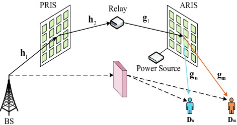
Figure 1: System model of PRIS-ARIS-NOMA.

II-A Signal Model

Although ARIS can use an external power source to combat the channel fading of signal propagation, it also leads to the amplification of noise signals on it, which cannot be idealized as in the analysis of a single PRIS model and the amplified noise from the transmitter on ARIS cannot be ignored in the analysis process. Hence, the expression of the received signal when it passes through the whole channel link and then is received at the $\varphi$-th user is denoted as

$${y_{\varphi}}=\sqrt{\beta}{\mathbf{g}}_{\varphi}^{H}{{\mathbf{\Phi}}_{a}} \left[{{\mathbf{h}}_{2}^{H}{{\mathbf{\Phi}}_{p}}{{\mathbf{h}}_{1}}\left({\sqrt{{a_{n}}{P_{s}^{a}}}{x_{n}}}\right.}\right.\hfill$$

$$\left.{\left.{+\sqrt{{a_{m}}{P_{s}}}{x_{m}}}\right)G{{\mathbf{g}}_{1}}+{{\mathbf{N}}_{a}}}\right]+{n_{0}},$$ (1)

where ${{\mathbf{\Phi}}_{a}}$ and ${{\mathbf{\Phi}}_{p}}$ represent the reflecting phase shift matrices of ARIS and PRIS, which have been given a detailed explanation and definition above. ${{\mathbf{N}}_{a}}\sim\mathcal{C}\mathcal{N}\left({0,\sigma_{a}^{2}{{\mathbf{I}}_{N}}}\right)$ represents the thermal noise, and ${\mathbf{I}}_{N}\in{\mathbb{C}^{M\times 1}}$ is a unit column vector. $a_{n}$ and $a_{m}$ are power allocation factor of $D_{n}$ and $D_{m}$, respectively, with $a_{n}+a_{m}=1$. $P_{s}^{a}$ is the transmitting power of the BS for PRIS-ARIS-NOMA with $x_{n}$ and $x_{m}$ are normalized power signals. For elaboration, $\mathbb{E}\left\{{{{\left|{{x_{n}}}\right|}^{2}}}\right\}=\mathbb{E}\left\{{{{\left|{{x_{m}}}\right|}^{2}}}\right\}=1$. Meanwhile, ${n_{0}}\sim\mathcal{C}\mathcal{N}(0,{\sigma^{2}})$ is the additive white Gaussian noise (AWGN) at the receiving end, ${\sigma^{2}}$ is the power of AWGN. $G$ is the AF amplification gain and set $G$ to 1 for calculations.

Rice fading channels and Nakagami-$m$ fading channels are the more commonly used channel modelling approaches in performance analysis scenarios and are commonly used to analyze and model signal transmission performance in wireless communication systems. The fading characteristics of the Rician fading channel consist mainly of fading from the dominant path, but also from the multipath component, and are therefore suitable for modelling the transmission channel between RISs in this model. The Nakagami-$m$ fading channel model is applicable to a variety of different wireless environments, including indoor, outdoor, urban and suburban areas, and is therefore well suited for the transmitting link as well as the receiving link in this model. In order to better fit the actual channel characteristics, we considered the channels from BS to PRIS ,then from ARIS to users as Nakagami-$m$ fading channels. Assuming the channels between the two RISs are Rician fading channels. Based on the above definition of the communication channels, we can denote the channel coefficients from BS to PRIS and PRIS to AF as ${{\bf{h}}_{1}}=\sqrt{\eta d_{h1}^{-\alpha}}\left[{h_{1}^{1},h_{2}^{1}\ldots,h_{N}^{1}}\right]^{H}$ and ${{\bf{h}}_{2}}=\sqrt{\eta d_{h2}^{-\alpha}}\left[{h_{1}^{2},h_{2}^{2}\ldots,h_{N}^{2}}\right]^{2}$, respectively. And meanwhile denote the channel coefficients from AF to ARIS and ARIS to the $\varphi$-user as ${{\bf{g}}_{1}}=\sqrt{\eta d_{g1}^{-\alpha}}{\left[{g_{1}^{1},g_{2}^{1}\ldots,g_{M}^{1}}\right]^{H}}$ and ${{\bf{g}}_{\varphi}}=\sqrt{\eta d_{g\varphi}^{-\alpha}}{\left[{g_{1}^{\varphi},g_{2}^{\varphi}\ldots,g_{M}^{\varphi}}\right]^{H}}$, respectively. $\eta$ expresses the the pass loss while $\alpha$ expresses the path loss exponent. $d_{h1}$,$d_{h2}$,$d_{g1}$,$d_{g\varphi}$ respectively denote the distance of each channel segment. $h_{n}^{1}$ and $g_{m}^{\varphi}$ follows the Nakagami-$m$ fading with shape parameter $m_{na}$ and scale parameter $\Omega_{na}$. $h_{n}^{2}=\sqrt{\frac{\kappa}{{\kappa+1}}}+\sqrt{\frac{1}{{\kappa+1}}}\widehat{h_{n}^{2}}$ and $g_{m}^{1}=\sqrt{\frac{\kappa}{{\kappa+1}}}+\sqrt{\frac{1}{{\kappa+1}}}\widehat{g_{m}^{1}}$, where $\widehat{g_{m}^{1}}$ and $\widehat{h_{n}^{2}}\sim{\mathcal{C}}{\mathcal{N}}\left({0,1}\right)$. $\kappa$ is the Rician factor, which represents the ratio of the LoS component power to the scattered component power. In order to make the analysis more accurate, all of the complex channel coefficients random variables which are from each part of channels are independent, and each part of channels is assumed to follow independent block fading, either. It is to be noted that the normalized signals power is taken in the following calculation.

On the basis of the NOMA protocol, the transmitting end sends the superposed signal to each pair of non-orthogonal users, and the receiving end starts SIC procedure for decoding the signals. The received signal-to-interference-plus-noise ratio (SINR) at $D_{n}$ to detected $D_{m}$’s information $x_{m}$ can be denoted by

$$\gamma_{{D_{n}}}^{{D_{m}}}=\frac{{\beta{P_{s}^{a}}{{\left|{{\bf{h}}_{2}^{H}{{\bf{\Phi}}_{p}}{{\bf{h}}_{1}}}\right|}^{2}}{{\left|{{\bf{g}}_{n}^{H}{{\bf{\Phi}}_{a}}{{\bf{g}}_{1}}}\right|}^{2}}{a_{m}}}}{{\beta{P_{s}^{a}}{{\left|{{\bf{h}}_{2}^{H}{{\bf{\Phi}}_{p}}{{\bf{h}}_{1}}}\right|}^{2}}{{\left|{{\bf{g}}_{n}^{H}{{\bf{\Phi}}_{a}}{{\bf{g}}_{1}}}\right|}^{2}}{a_{n}}+\beta\sigma_{a}^{2}{{\left\|{{\bf{g}}_{n}^{H}{{\bf{\Phi}}_{a}}}\right\|}^{2}}+{\sigma^{2}}}}.$$ (2)

After $D_{n}$ decoded and subtracted $D_{m}$’s signals $x_{m}$, it would next decode its own signals $x_{n}$. The received SINR at $D_{n}$ to detect its own information $x_{n}$ can be denoted by

$${\gamma_{{D_{n}}}}=\frac{{\beta{P_{s}^{a}}{{\left|{{\bf{h}}_{2}^{H}{{\bf{\Phi}}_{p}}{{\bf{h}}_{1}}}\right|}^{2}}{{\left|{{\bf{g}}_{n}^{H}{{\bf{\Phi}}_{a}}{{\bf{g}}_{1}}}\right|}^{2}}{a_{n}}}}{{\varpi{P_{s}^{a}}{{\left|{{h_{RI}}}\right|}^{2}}+\beta\sigma_{a}^{2}{{\left\|{{\bf{g}}_{n}^{H}{{\bf{\Phi}}_{a}}}\right\|}^{2}}+{\sigma^{2}}}},$$ (3)

where $\varpi={\text{0 or 1}}$ represents the pSIC and ipSIC operation during the SIC process, respectively. ${h_{RI}}\sim\mathcal{C}\mathcal{N}\left({0,{\Omega_{RI}}}\right)$ represents the corresponding complex coefficient of the residual interference during the ipSIC operation. Noted that the generation of ipSIC is mainly due to the imperfect design of the SIC receiver as well as hardware errors, whereas in this paper we use the mathematical modelling of stochastic processes to model the mathematical properties of the whole channel, so that the CSI case received by the users can be assumed to be perfect.

When it comes to $D_{m}$’s demodulation part, the information belonged to $D_{n}$ is treated as interference during the SIC process. Therefore, the received SINR at $D_{m}$ to detected its own information $x_{m}$ can be denoted by

$${\gamma_{{D_{m}}}}=\frac{{\beta{P_{s}^{a}}{{\left|{{\bf{h}}_{2}^{H}{{\bf{\Phi}}_{p}}{{\bf{h}}_{1}}}\right|}^{2}}{{\left|{{\bf{g}}_{m}^{H}{{\bf{\Phi}}_{a}}{{\bf{g}}_{1}}}\right|}^{2}}{a_{m}}}}{{\beta{P_{s}^{a}}{{\left|{{\bf{h}}_{2}^{H}{{\bf{\Phi}}_{p}}{{\bf{h}}_{1}}}\right|}^{2}}{{\left|{{\bf{g}}_{m}^{H}{{\bf{\Phi}}_{a}}{{\bf{g}}_{1}}}\right|}^{2}}{a_{n}}+\beta\sigma_{a}^{2}{{\left\|{{\bf{g}}_{m}^{H}{{\bf{\Phi}}_{a}}}\right\|}^{2}}+{\sigma^{2}}}}.$$ (4)

In order to provide a comparative basis for one of the experimental results, OMA scheme was presented as a baseline for comparison with NOMA scheme. The SNR at the nearby user $D_{n}$ and distant user $D_{m}$ under OMA scheme can be given by

$$\gamma_{{D_{n}}}^{OMA}=\frac{{\beta{P_{s}}{a_{n}}{{\left|{{\bf{h}}_{2}^{H}{{\bf{\Phi}}_{p}}{{\bf{h}}_{1}}}\right|}^{2}}{{\left|{{\bf{g}}_{n}^{H}{{\bf{\Phi}}_{a}}{{\bf{g}}_{1}}}\right|}^{2}}}}{{\beta\sigma_{a}^{2}{{\left\|{{\bf{g}}_{n}^{H}{{\bf{\Phi}}_{a}}}\right\|}^{2}}+{\sigma^{2}}}}$$ (5)

and

$$\gamma_{{D_{m}}}^{OMA}=\frac{{\beta{P_{s}}{a_{m}}{{\left|{{\bf{h}}_{2}^{H}{{\bf{\Phi}}_{p}}{{\bf{h}}_{1}}}\right|}^{2}}{{\left|{{\bf{g}}_{m}^{H}{{\bf{\Phi}}_{a}}{{\bf{g}}_{1}}}\right|}^{2}}}}{{\beta\sigma_{a}^{2}{{\left\|{{\bf{g}}_{m}^{H}{{\bf{\Phi}}_{a}}}\right\|}^{2}}+{\sigma^{2}}}},$$ (6)

respectively.

II-B Channel Statistical Properties

In order to further improve the performance the networks, coherent phase shifting scheme has been adopted to optimize the phase shifting process [49]. In a coherent phase shifting scheme, the phase shifts of each reflecting and transmitting element are synchronized with the phases of their respective incoming and outgoing fading channels. This coherence results in superior analytical performance compared to the random phase shifting scheme. It can simulate a more idealized and better channel state, and can reflect the system characteristics more intuitively and conveniently. In coherent phase shifting scheme, when the distance is normalized, we can define the cascade channel gain ${\left|{{\bf{h}}_{2}^{H}{\bf{\Theta}}{{\bf{h}}_{1}}}\right|^{2}}$ as ${\zeta_{h}}={\left|{\sum\nolimits_{n=1}^{N}{\left|{h_{n}^{1}h_{n}^{2}}\right|}}\right|^{2}}$, and define ${\left|{{\bf{g}}_{\varphi}^{H}{\bf{\Theta}}{{\bf{g}}_{1}}}\right|^{2}}$ as ${\zeta_{g}}={\left|{\sum\nolimits_{m=1}^{M}{\left|{g_{m}^{1}g_{m}^{\varphi}}\right|}}\right|^{2}}$. Let ${X_{n}}=\left|{h_{n}^{1}h_{n}^{2}}\right|$ and $X_{m}^{\varphi}=\left|{g_{m}^{1}g_{m}^{\varphi}}\right|$, thus we can get the PDF for a single cascaded Rician fading and Nakagami-$m$ fading channel as

$${f_{{X_{n}}}}\left(y\right)={f_{{X_{m}^{\varphi}}}}\left(y\right)= \sum\limits_{m=0}^{\infty}{\frac{{4{y^{m+{m_{na}}}}{\kappa^{m}}{{\left[{\frac{{\left({\kappa+1}\right){m_{na}}}}{{\hat{r}_{1}^{2}{{\hat{r}}_{2}}}}}\right]}^{\frac{{1+m+{m_{na}}}}{2}}}}}{{{e^{\kappa}}{{\left({m!}\right)}^{2}}\Gamma\left({{m_{na}}}\right)}}}\hfill$$

$$\times{K_{m-{m_{na}}+1}}\left({2y\sqrt{\frac{{\left({\kappa+1}\right){m_{na}}}}{{\hat{r}_{1}^{2}{{\hat{r}}_{2}}}}}}\right),$$ (7)

where ${\hat{r}_{i}}$ is the root-mean square value of the received signal envelope ${R_{i}}$ [50], $\Gamma(\cdot)$ is the gamma function[51, Eq. (8.310.1)]. ${K_{\phi}}(\cdot)$ is the $\phi$th-order modified Bessel function of the second kind[51, Eq. (8.432)].

Since all channel parameters are distributed independently, $X_{n}$ and $X_{m}$ have the same mean and variance, which can be given by

$${e_{\varphi}}=\sqrt{\frac{\pi}{{4\left({\kappa+1}\right)}}}\frac{{\Gamma\left({{m_{na}}+\frac{1}{2}}\right)}}{{\Gamma\left({{m_{na}}}\right)}}{\left({\frac{1}{{{m_{na}}}}}\right)^{\frac{1}{2}}}{L_{\frac{1}{2}}}\left({-\kappa}\right),$$ (8)

and

$${d_{\varphi}}=1-\frac{{L_{\frac{1}{2}}^{2}\left({-\kappa}\right)}}{{4\left({\kappa+1}\right)}}\left[{\frac{\pi}{m}{{\left({\frac{{\Gamma\left({m+\frac{1}{2}}\right)}}{{\Gamma\left(m\right)}}}\right)}^{2}}}\right],$$ (9)

respectively, where ${L_{\frac{1}{2}}}\left(x\right)$ is the Laguerre polynomial and ${L_{\frac{1}{2}}}\left({-\kappa}\right)={e^{-\frac{\kappa}{2}}}\left[{\left({1+\kappa}\right){I_{0}}\left({\frac{\kappa}{2}}\right)+\kappa{I_{1}}\left({\frac{\kappa}{2}}\right)}\right]$, where ${I_{0}}\left(\cdot\right)$ and ${I_{1}}\left(\cdot\right)$ are respectively the modified zeroth-order and first-order Bessel function of the first kind.

Then, with the help of Laguerre polynomial series[52, Sec. 2.2.2], the approximate PDF of ${\zeta_{h}}$ and ${\zeta_{g}}$ can be given by

$${f_{{\zeta_{h}}}}\left(x\right)=\frac{{{x^{\frac{{{a_{X}}-1}}{2}}}}}{{2{b^{{a_{X}}+1}}\Gamma\left({{a_{X}}+1}\right)}}{e^{-\frac{{\sqrt{x}}}{{{b_{X}}}}}},$$ (10)

and

$${f_{{\zeta_{g}}}}\left(y\right)=\frac{{{y^{\frac{{{a_{Y}}-1}}{2}}}}}{{2{b^{{a_{Y}}+1}}\Gamma\left({{a_{Y}}+1}\right)}}{e^{-\frac{{\sqrt{y}}}{{{b_{Y}}}}}},$$ (11)

respectively, where ${a_{X}}=\frac{{Ne_{\varphi}^{2}}}{{{d_{\varphi}}}}-1$, ${a_{Y}}=\frac{{Me_{\varphi}^{2}}}{{{d_{\varphi}}}}-1$,${b_{X}}={b_{Y}}=\frac{{{d_{\varphi}}}}{{{e_{\varphi}}}}$.

III Outage Probability

This section evaluates the performance of the PRIS-ARIS-NOMA in the perspective of outage probability. In this section the outage probability expressions for $D_{n}$ with ipSIC/pSIC and $D_{m}$ are derived in detail. And the outage probability expressions of $D_{n}$ with ipSIC/pSIC and $D_{m}$ at high SNR region are further derived based on the outage probability expressions.

III-A The Outage Probability of $D_{n}$

According to the regulations of SIC process, the weak user needs to decode and discard the signals of the strong user, i.e., the signals of $D_{m}$, before decoding its own signals in the SIC process. Therefore, the event that causes an outage to $D_{n}$ can be defined as:1) If $D_{n}$ cannot detect the signals $x_{m}$ from $D_{m}$, then an outage occurs at $D_{n}$. 2) If $D_{n}$ can detect and decode $D_{m}$’s signal $x_{m}$, but cannot detect and decode its own signal $x_{n}$, then an outage occurs at $D_{n}$. Based on the above representations, the outage probability of $D_{n}$ in PRIS-ARIS-NOMA can be denoted as

$$P_{{D_{n}}}^{out}=\Pr\left({\gamma_{{D_{n}}}^{{D_{m}}}<{\gamma_{t{h_{m}}}}}\right)+\Pr\left({\gamma_{{D_{n}}}^{{D_{m}}}>{\gamma_{t{h_{m}}}},{\gamma_{{D_{n}}}}<{\gamma_{t{h_{n}}}}}\right),$$ (12)

where ${\gamma_{t{h_{n}}}}={2^{{R_{n}}}}-1$ and ${\gamma_{t{h_{m}}}}={2^{{R_{m}}}}-1$ are respectively the target SNR threshold when detecting signals. And $R_{n}$ and $R_{m}$ are respectively the instantaneous target rate threshold for $D_{n}$ and $D_{m}$.

Theorem 1.

Under cascaded Rician fading and Nakagami-$m$ fading channels, the closed-form expression for outage probability of $D_{n}$ with ipSIC for PRIS-ARIS-NOMA can be expressed as

$$P_{{D_{n}}}^{out,ipSIC}=\sum\limits_{i=1}^{I}{\sum\limits_{u=1}^{U}{\frac{{{H_{i}}{H_{u}}x_{u}^{{a_{X}}}}}{{\Gamma({a_{X}}+1)\Gamma({a_{Y}}+1)}}}}\hfill$$

$$\times\gamma\left({{a_{Y}}+1,\frac{{\sqrt{\overline{{\lambda_{n}}}{\gamma_{t{h_{n}}}}\left({\varpi{P_{s}^{a}}{\Omega_{RI}}{x_{i}}+\beta\sigma_{a}^{2}M{\Omega_{na}}+{\sigma^{2}}}\right)}}}{{\sqrt{\beta{P_{s}^{a}}{a_{n}}}{b_{X}}{b_{Y}}{x_{u}}}}}\right),$$ (13)

where $\varpi=1$, $\overline{{\lambda_{n}}}={\eta^{-4}}d_{h1}^{\alpha}d_{h2}^{\alpha}d_{g1}^{\alpha}d_{gn}^{\alpha}$. For bringing into Gauss-Laguerre quadrature, ${{x_{u}}}$ is the $u$-th zero point of Laguerre polynomial ${L_{u}}({x_{u}})$ and ${{x_{i}}}$ is the $i$-th zero point of Laguerre polynomial ${L_{i}}({x_{i}})$. ${{H_{u}}}$ is the $u$-th weight, and can be denoted by ${H_{u}}=\frac{{{{[(U+1)!]}^{2}}}}{{{x_{u}}{{[{{L^{\prime}}_{U+1}}({x_{u}})]}^{2}}}},u=0,1,...,U$. Similarly, ${{H_{i}}}$ get the same mathematical meaning as ${{H_{u}}}$ and can be denoted by ${H_{i}}=\frac{{{{[(I+1)!]}^{2}}}}{{{x_{i}}{{[{{L^{\prime}}_{I+1}}({x_{i}})]}^{2}}}},i=0,1,...,I$. Specifically, ${L_{\varphi}}\left(x\right)={e^{x}}\frac{{{d^{\varphi}}}}{{d{x^{\varphi}}}}\left({{x^{\varphi}}{e^{-x}}}\right)$ is $\varphi$-th order Laguerre polynomial and ${L_{\varphi}}^{\prime}\left(x\right)$ is the derivative of ${L_{\varphi}}\left(x\right)$. ${\gamma(\alpha,x)=\int_{0}^{x}{{e^{-t}}{t^{\alpha-1}}}dt}$ is the lower incomplete Gamma function[51, Eq. (8.350.1)]. Particularly, formula is valid under the condition of ${{a_{m}}>{\gamma_{t{h_{m}}}}{a_{n}}}$, if ${{a_{m}}<{\gamma_{t{h_{m}}}}{a_{n}}}$, then the nearby user will always be in the outage state.

Proof.

See Appendix A. ∎

Corollary 1.

When it comes to the special case of $\varpi=0$, the closed-formed expression for outage probability of $D_{n}$ with pSIC for PRIS-ARIS-NOMA can be expressed as

$$P_{{D_{n}}}^{out,pSIC}= \sum\limits_{u=1}^{U}{\frac{{{H_{u}}x_{u}^{{a_{X}}}}}{{\Gamma({a_{X}}+1)\Gamma({a_{Y}}+1)}}}\hfill$$

$$\times\gamma\left({{a_{Y}}+1,\frac{{\sqrt{\overline{{\lambda_{n}}}{\gamma_{t{h_{n}}}}\left({\beta\sigma_{a}^{2}M{\Omega_{na}}+{\sigma^{2}}}\right)}}}{{\sqrt{\beta P_{s}^{a}{a_{n}}}{b_{X}}{b_{Y}}{x_{u}}}}}\right).$$ (14)

III-B The Outage Probability of $D_{m}$

In NOMA scenario, for distant user during the SIC process, only its own signals need to be decoded and the signals of the nearby user are treated as interference. Therefore, the event that causes an outage to $D_{m}$ can be defined as: If $D_{m}$ cannot detect the signals $x_{m}$ itself, then an outage occurs at $D_{m}$. Based on the above representations, the outage probability of $D_{m}$ in PRIS-ARIS-NOMA can be denoted as

$$P_{{D_{m}}}^{out}=\Pr\left({{\gamma_{{D_{m}}}}<{\gamma_{t{h_{m}}}}}\right).$$ (15)

Theorem 2.

Under cascaded Rician fading and Nakagami-$m$ fading channels, the closed-form expression for outage probability of $D_{m}$ for PRIS-ARIS-NOMA can be expressed as

$$P_{{D_{m}}}^{out}= \sum\limits_{u=1}^{U}{\frac{{{H_{u}}x_{u}^{{a_{X}}}}}{{\Gamma({a_{X}}+1)\Gamma({a_{Y}}+1)}}}\hfill$$

$$\times\gamma\left({{a_{Y}}+1,\frac{{\sqrt{\overline{{\lambda_{m}}}{\gamma_{t{h_{m}}}}\left({\beta\sigma_{a}^{2}M{\Omega_{na}}+{\sigma^{2}}}\right)}}}{{\sqrt{\beta{P_{s}^{a}}\left({{a_{m}}-{\gamma_{t{h_{m}}}}{a_{n}}}\right)}{b_{X}}{b_{Y}}{x_{u}}}}}\right),$$ (16)

where $\overline{{\lambda_{m}}}={\eta^{-4}}d_{h1}^{\alpha}d_{h2}^{\alpha}d_{g1}^{\alpha}d_{gm}^{\alpha}$, ${{a_{m}}>{\gamma_{t{h_{m}}}}{a_{n}}}$.

Proof.

By substituting (4) into (15), the outage probability expression of $D_{m}$ can be further derived as (17) at the top of the next page.

$$P_{{D_{m}}}^{out} =\Pr\left({\frac{{\beta{P_{s}^{a}}{{\left|{{\mathbf{h}}_{2}^{T}{{\mathbf{\Phi}}_{p}}{{\mathbf{h}}_{1}}}\right|}^{2}}{{\left|{{\mathbf{g}}_{m}^{T}{{\mathbf{\Phi}}_{a}}{{\mathbf{g}}_{1}}}\right|}^{2}}{a_{m}}}}{{\beta{P_{s}^{a}}{{\left|{{\mathbf{h}}_{2}^{T}{{\mathbf{\Phi}}_{p}}{{\mathbf{h}}_{1}}}\right|}^{2}}{{\left|{{\mathbf{g}}_{m}^{T}{{\mathbf{\Phi}}_{a}}{{\mathbf{g}}_{1}}}\right|}^{2}}{a_{n}}+\beta\sigma_{a}^{2}{{\left\|{{\mathbf{g}}_{n}^{T}{{\mathbf{\Phi}}_{a}}}\right\|}^{2}}+{\sigma^{2}}}}<{\gamma_{t{h_{m}}}}}\right).$$ (17)

The remaining computational steps of the proof are similar to the proof steps in Appendix A. The proof is completed. ∎

III-C The Outage Probability of the OMA Benchmark

In this paper, the OMA scheme is set up as one of the benchmarks for comparison with the NOMA scheme under the double RISs assisted networks. For OMA scheme, the transmission of users’informations throughout the system is orthogonal in the frequency domain, and in a dual users system, it can be assumed that each of the two users occupies half of the frequency domain resources. For OMA scheme, an outage occurs when the user’s received SNR is less than the set SNR threshold, which can be expressed as

$$P_{{D_{\varphi}}}^{OMA}=\Pr\left({\gamma_{{D_{\varphi}}}^{OMA}<\gamma_{t{h_{\varphi}}}^{OMA}}\right),$$ (18)

where $\gamma_{t{h_{\varphi}}}^{OMA}={2^{2{R_{\varphi}}}}-1$ represents the target SNR threshold when detecting the $\varphi$-th user’s signals, and $R_{\varphi}$ is the instantaneous target rate threshold for the $\varphi$-th user. Similar to the above derivation process, the outage probabilities for the two users under double RISs assisted OMA networks are presented in the following theorem.

Theorem 3.

Under Rician fading and Nakagami-$m$ fading cascaded channels, the approximated closed-form expression for outage probability of the $\varphi$-th user for double RISs assisted OMA networks can be expressed as

$$P_{{D_{\varphi}}}^{OMA}= \sum\limits_{u=1}^{U}{\frac{{{H_{u}}x_{u}^{{a_{X}}}}}{{\Gamma({a_{X}}+1)\Gamma({a_{Y}}+1)}}}\hfill$$

$$\times\gamma\left({{a_{Y}}+1,\frac{{\sqrt{\overline{{\lambda_{\varphi}}}\gamma_{t{h_{\varphi}}}^{OMA}\left({\beta\sigma_{a}^{2}M{\Omega_{na}}+{\sigma^{2}}}\right)}}}{{\sqrt{\beta{P_{s}^{a}}{a_{\varphi}}}{b_{X}}{b_{Y}}{x_{u}}}}}\right),$$ (19)

where $\varphi\in\left\{{m,n}\right\}$.

III-D Diversity Analysis

Diversity order is an important metric for measuring system communication performance and describes how fast the outage probability decreases with an increasing SNR [53]. The diversity order can be expressed as the ratio of the asymptotic outage probability in the high SNR region, which can be expressed as

$$\mathop{\lim}\limits_{{P_{s}^{a}}\to\infty}-\frac{{\log P_{out}^{\infty}\left({{P_{s}^{a}}}\right)}}{{\log{P_{s}^{a}}}},$$ (20)

where ${P_{out}^{\infty}\left({{P_{s}^{a}}}\right)}$ represents the asymptotic outage probability at high SNR region, .i.e, ${{P_{s}^{a}}\to\infty}$. The asymptotic outage probability of $D_{n}$ with ipSIC can be directly deduced from (1) and leads to the following corollary.

Corollary 2.

When ${{P_{s}^{a}}\to\infty}$, the expression for asymptotic outage probability of $D_{n}$ with ipSIC for PRIS-ARIS-NOMA under cascaded Rician fading and Nakagami-$m$ fading channels can be expressed as

$$P_{out,{D_{n}}}^{\infty,ipSIC}= \sum\limits_{i=1}^{I}{\sum\limits_{u=1}^{U}{\frac{{{H_{i}}{H_{u}}x_{u}^{{a_{X}}}}}{{\Gamma({a_{X}}+1)\Gamma({a_{Y}}+1)}}}}\hfill$$

$$\times\gamma\left({{a_{Y}}+1,\frac{{\sqrt{\overline{{\lambda_{n}}}{\gamma_{t{h_{n}}}}{\Omega_{RI}}{x_{i}}}}}{{\sqrt{\beta{a_{n}}}{b_{X}}{b_{Y}}{x_{u}}}}}\right).$$ (21)

Remark 1.

From Corollary2, it can be deduced that the outage probability of $D_{n}$ with ipSIC will gradually converge to a constant as SNR tends to infinity. By substituting (2) into (20), a zero diversity order for $D_{n}$ with ipSIC can be derived. The reason for this phenomenon is that the residual interference during the ipSIC process limits the user acceptance performance improvement as the SNR increases, thus causing the outage performance to converge to a constant state.

Corollary 3.

With the condition of $N=M$, when ${{P_{s}^{a}}\to\infty}$, the expression for asymptotic outage probability of $D_{n}$ with pSIC for PRIS-ARIS-NOMA under cascaded Rician fading and Nakagami-$m$ fading channels can be expressed as (22) at the top of the next page.

$$P_{out,{D_{n}}}^{\infty,pSIC}=\frac{{\pi{\mu_{b}}{{\left({\overline{{\lambda_{n}}}{\gamma_{t{h_{n}}}}}\right)}^{M}}{{\left({\beta\sigma_{a}^{2}M{\Omega_{na}}+{\sigma^{2}}}\right)}^{M}}}}{{2K\left({2M}\right)!\left({2N-1}\right)!{{\left({\beta{P_{s}}{a_{n}}}\right)}^{M}}}}{\left[{\frac{{4\sqrt{\pi}\Gamma\left({2{m_{na}}}\right)\Delta\left(0\right)}}{{{e^{\kappa}}\Gamma\left({{m_{na}}}\right)}}}\right]^{M+N}}\sum\limits_{k=1}^{K}{{{\left[{\frac{{\left({{x_{k}}{\text{ + }}1}\right){\mu_{b}}}}{2}}\right]}^{2N-2M-1}}\sqrt{1-{x_{k}^{2}}}}.$$ (22)

Where $K$ is the parameter of the Gauss-Chebyshev quadrature formula for precision. $\mu_{b}$ is the upper limit of integral before using the Gauss-Chebyshev quadrature formula for the approximation and ${\mu_{b}}\to\infty$. ${x_{k}}=\cos\left({\frac{{2k-1}}{{2K}}\pi}\right)$. $\Delta\left(0\right)$ is given as following where $F\left({\cdot,\cdot;\cdot;\cdot}\right)$ is the Gauss hypergeometric function[51, Eq. (9.100)].

$$\Delta\left(0\right)= \frac{{{{\left({4\sqrt{\left({\kappa+1}\right){m_{na}}}}\right)}^{1-{m_{na}}}}{{\left[{\left({\kappa+1}\right){m_{na}}}\right]}^{\frac{1}{2}\left({1+{m_{na}}}\right)}}}}{{\Gamma\left({{m_{na}}+\frac{3}{2}}\right)}}\hfill$$

$$\times F\left({2,\frac{3}{2}-{m_{na}};{m_{na}}+\frac{3}{2};1}\right)$$ (23)

Proof.

See Appendix B. ∎

Remark 2.

From Corollary 3, it can be deduced that the asymptotic outage probability of $D_{n}$ with pSIC is an oblique line that decreases as SNR increases. By substituting (22) into (20), the diversity order of $D_{n}$ with pSIC can be derived as $M$, which is related to the number of the ARIS’s reflecting elements.

Corollary 4.

In the same analogy with the process of solving (22), the expression for asymptotic outage probability of $D_{m}$ for PRIS-ARIS-NOMA under cascaded Rician fading and Nakagami-$m$ fading channels can be expressed as (24) at the top of the next page.

$$P_{out,{D_{m}}}^{\infty}=\frac{{\pi{\mu_{b}}{{\left({\overline{{\lambda_{m}}}{\gamma_{t{h_{m}}}}}\right)}^{M}}{{\left({\beta\sigma_{a}^{2}M{\Omega_{na}}+{\sigma^{2}}}\right)}^{M}}}}{{2K\left({2M}\right)!\left({2N-1}\right)!{{\left[{\beta{P_{s}}\left({{a_{m}}-{\gamma_{t{h_{m}}}}{a_{n}}}\right)}\right]}^{M}}}}{\left[{\frac{{4\sqrt{\pi}\Gamma\left({2{m_{na}}}\right)\Delta\left(0\right)}}{{{e^{\kappa}}\Gamma\left({{m_{na}}}\right)}}}\right]^{M+N}}\sum\limits_{k=1}^{K}{{{\left[{\frac{{\left({{x_{k}}{\text{ + }}1}\right){\mu_{b}}}}{2}}\right]}^{2N-2M-1}}\sqrt{1-{x_{k}^{2}}}}.$$ (24)

Proof.

The proof process of this corollary can be referred to the proof process of Corollary 3 in Appendix B. ∎

Remark 3.

By substituting (24) into (20), the diversity order of $D_{m}$ can be derived as $M$, which is related to the number of the ARIS’s reflecting elements.

III-E Delay-limited Transmission

In delay-limited transmission scheme, the BS sends signals at a constant power but the system throughput is subject to the outage probability of each user [54]. Therefore, the system throughput for PRIS-ARIS-NOMA under cascaded Rician fading and Nakagami-$m$ fading channels can be expressed as

$$R_{\varpi}^{{\text{limited}}}=\left({1-P_{{D_{n}}}^{out,\varpi}}\right){R_{n}}+\left({1-P_{{D_{m}}}^{out}}\right){R_{m}},$$ (25)

where $\varpi$ means ipSIC/pSIC scheme, $P_{{D_{n}}}^{out,ipSIC}$, $P_{{D_{n}}}^{out,pSIC}$ and $P_{{D_{m}}}^{out}$ can respectively be obtained from (1), (1) and (2).

IV Ergodic Data Rate Analysis

The ergodic data rate is another important performance evaluation metric for wireless communication systems. It is the maximum rate at which the code of the transmitting signals can traverse all fading states, i.e., the maximum rate at which the system can transmit signals correctly in a fading channel. And the definition of the ergodic data rate can be expressed as

$${R^{ergodic}}=\mathbb{E}\left[{{{\log}_{2}}\left({1+\gamma}\right)}\right],$$ (26)

where $\gamma$ means the SINR for users. In this section the ergodic data rate expressions for $D_{n}$ with ipSIC/pSIC and $D_{m}$ are derived in detail. And we further derived the ergodic data rate slope expressions of $D_{n}$ and $D_{m}$.

IV-A The Ergodic Data Rates of $D_{n}$

When solving for the ergodic data rate of $D_{n}$, we assume that $D_{n}$ can successfully detect and decode the signals of $D_{m}$, then the ergodic data rate expression of $D_{n}$ with ipSIC can be given in the following theorem.

Theorem 4.

Under cascaded Rician fading and Nakagami-$m$ fading channels, the closed-form expression for ergodic data rate of $D_{n}$ with ipSIC for PRIS-ARIS-NOMA can be expressed as

$$R_{Dn,ipSIC}^{ergodic}= \sum\limits_{p=1}^{P}{\sum\limits_{i=1}^{I}{\sum\limits_{u=1}^{U}{\frac{{{H_{p}}{H_{i}}{H_{u}}x_{u}^{{a_{X}}}x_{p}^{{a_{Y}}}}}{{\ln 2\Gamma({a_{X}}+1)\Gamma({a_{Y}}+1)}}}}}\hfill$$

$$\times\ln\left({1+\frac{{\beta{P_{s}^{a}}{a_{n}}b_{X}^{2}b_{Y}^{2}x_{u}^{2}x_{p}^{2}}}{{{{\bar{\lambda}}_{n}}\left({\varpi{P_{s}^{a}}{\Omega_{RI}}{x_{i}}+\beta\sigma_{a}^{2}M{\Omega_{na}}+{\sigma^{2}}}\right)}}}\right),$$ (27)

where $x_{p}$ and $H_{p}$ are the parameters of Gauss-Laguerre quadrature formula and both of the two parameters share the same meaning with ${x_{u}},{x_{i}}$ and ${H_{u}},{H_{i}}$ ,respectively.

Proof.

See Appendix C. ∎

Corollary 5.

When it comes to the special case of $\varpi=0$, the closed-formed expression for ergodic data rate of $D_{n}$ with pSIC for PRIS-ARIS-NOMA can be expressed as

$$R_{Dn,ipSIC}^{ergodic}= \sum\limits_{p=1}^{P}{\sum\limits_{u=1}^{U}{\frac{{{H_{p}}{H_{u}}x_{u}^{{a_{X}}}x_{p}^{{a_{Y}}}}}{{\ln 2\Gamma({a_{X}}+1)\Gamma({a_{Y}}+1)}}}}\hfill$$

$$\times\ln\left({1+\frac{{\beta P_{s}^{a}{a_{n}}b_{X}^{2}b_{Y}^{2}x_{u}^{2}x_{p}^{2}}}{{{{\bar{\lambda}}_{n}}\left({\beta\sigma_{a}^{2}M{\Omega_{na}}+{\sigma^{2}}}\right)}}}\right).$$ (28)

IV-B The Ergodic Data Rates of $D_{m}$

Similar to the method used for solving the ergodic data rate of $D_{n}$, the ergodic data rate expression of $D_{m}$ can be given in the following theorem.

Theorem 5.

Under cascaded Rician fading and Nakagami-$m$ fading channels, the closed-form expression for ergodic data rate of $D_{m}$ for PRIS-ARIS-NOMA can be expressed as

$$R_{{D_{m}}}^{ergodic}=\sum\limits_{k=1}^{K}{{\delta_{k}}\left[{1-\sum\limits_{u=1}^{U}{\frac{{{H_{u}}x_{u}^{{a_{X}}}}}{{\Gamma({a_{X}}+1)\Gamma({a_{Y}}+1)}}}}\right.}\hfill$$

$$\times\left.{\gamma\left({{a_{Y}}+1,\frac{{\sqrt{\overline{{\lambda_{m}}}\left({\beta\sigma_{a}^{2}M{\Omega_{na}}+{\sigma^{2}}}\right)\left({{x_{k}}+1}\right){a_{m}}}}}{{\sqrt{{a_{m}}{a_{n}}\beta{P_{s}^{a}}\left({1-{x_{k}}}\right)}{b_{X}}{b_{Y}}{x_{u}}}}}\right)}\right],$$ (29)

where ${\delta_{k}}=\frac{{\pi{a_{m}}\sqrt{1-x_{k}^{2}}}}{{K\ln 2\left[{2{a_{n}}+{a_{m}}\left({{x_{k}}{\text{ + }}1}\right)}\right]}}$.

Proof.

See Appendix D. ∎

IV-C The Ergodic Data Rates of OMA benchmark

Corollary 6.

Under Rician fading and Nakagami-$m$ fading cascaded channels, the closed-form expression for ergodic rate of the $\varphi$-th user for double RISs assisted OMA networks can be expressed as

$$R_{{D_{\varphi}},OMA}^{ergodic}= \sum\limits_{p=1}^{P}{\sum\limits_{u=1}^{U}{\frac{{{H_{p}}{H_{u}}x_{u}^{{a_{X}}}x_{p}^{{a_{Y}}}}}{{2\ln 2\Gamma({a_{X}}+1)\Gamma({a_{Y}}+1)}}}}\hfill$$

$$\times\ln\left({1+\frac{{\beta P_{s}^{a}{a_{\varphi}}b_{X}^{2}b_{Y}^{2}x_{u}^{2}x_{p}^{2}}}{{{{\bar{\lambda}}_{\varphi}}\left({\beta\sigma_{a}^{2}M{\Omega_{na}}+{\sigma^{2}}}\right)}}}\right).$$ (30)

IV-D Slope Analysis

The ergodic data rate slope is another important metric for the performance of the networks to assess the evolution of ergodic data rate with the transmitting SNR, which can be captured from the ergodic data rate at high SNR region and defined as

$$S=\mathop{\lim}\limits_{{P_{s}^{a}}\to\infty}\frac{{{R^{ergodic,\infty}}\left({{P_{s}^{a}}}\right)}}{{\log{P_{s}^{a}}}},$$ (31)

where ${{R^{ergodic,\infty}}\left({{P_{s}^{a}}}\right)}$ represents the asymptotic ergodic data rate at high SNR region.

IV-D1 Slope analysis of $D_{n}$ with ipSIC

On the basis of (4), the expression of asymptotic ergodic data rate of $D_{n}$ with ipSIC for PRIS-ARIS-NOMA at high SNR region, i.e. ${{P_{s}}\to\infty}$, can be derived as

$$R_{{D_{n}},ipSIC}^{ergodic,\infty}=\sum\limits_{p=1}^{P}{\sum\limits_{i=1}^{I}{\sum\limits_{u=1}^{U}{\frac{{{H_{p}}{H_{i}}{H_{u}}x_{u}^{{a_{X}}}x_{p}^{{a_{Y}}}\ln\left({1+\frac{{\beta{a_{n}}b_{X}^{2}b_{Y}^{2}x_{u}^{2}x_{p}^{2}}}{{{{\bar{\lambda}}_{n}}{\Omega_{RI}}{x_{i}}}}}\right)}}{{\ln 2\Gamma({a_{X}}+1)\Gamma({a_{Y}}+1)}}}}}.$$ (32)

Remark 4.

By substituting (32) into (31), a zero ergodic data rate slope for $D_{n}$ with ipSIC can be derived, which means that the residual interference during the ipSIC process limits the user’s performance and causes the ergodic data rate to converge to a constant value when SNR increases.

IV-D2 Slope analysis of $D_{n}$ with pSIC

With the help of Jensen’s inequality written as $E\left[{{{\log}_{2}}\left({1+{\gamma_{{D_{n}}}}}\right)}\right]\leqslant{\log_{2}}\left[{1+E\left({{\gamma_{{D_{n}}}}}\right)}\right]$, we can obtain the upper bound of ergodic data rate of $D_{n}$ with pSIC for PRIS-ARIS-NOMA when ${{P_{s}}\to\infty}$ as

$$R_{{D_{n}},pSIC}^{ergodic,up} ={\log_{2}}\left[{1+\mathbb{E}\left({\frac{{\beta{P_{s}^{a}}{{\left|{{\mathbf{h}}_{2}^{T}{{\mathbf{\Phi}}_{p}}{{\mathbf{h}}_{1}}}\right|}^{2}}{{\left|{{\mathbf{g}}_{n}^{T}{{\mathbf{\Phi}}_{a}}{{\mathbf{g}}_{1}}}\right|}^{2}}{a_{n}}}}{{\beta\sigma_{a}^{2}{{\left\|{{\mathbf{g}}_{n}^{T}{{\mathbf{\Phi}}_{a}}}\right\|}^{2}}+{\sigma^{2}}}}}\right)}\right]\hfill$$

$$={\log_{2}}\left[{1+\frac{{{\vartheta_{n}}\beta{P_{s}^{a}}{a_{n}}{{\left({\overline{{\lambda_{n}}}}\right)}^{-1}}}}{{\beta\sigma_{a}^{2}M{\Omega_{na}}+{\sigma^{2}}}}}\right],$$ (33)

where ${\vartheta_{n}}=\left[{{{\left({N{e_{\varphi}}}\right)}^{2}}+N{d_{\varphi}}}\right]\left[{{{\left({M{e_{\varphi}}}\right)}^{2}}+M{d_{\varphi}}}\right]$, and ${{e_{\varphi}}}$ and ${{d_{\varphi}}}$ can be obtained from (8) and (9).

Remark 5.

By substituting (IV-D2) into (31), we can obtain that the ergodic data rate slope for $D_{n}$ with pSIC is equal to $1$.

IV-D3 Slope analysis of $D_{m}$

On the basis of (5), the expression of asymptotic ergodic data rate of $D_{m}$ for PRIS-ARIS-NOMA in the high SNR region, i.e. ${{P_{s}^{a}}\to\infty}$, can be derived as

$$R_{{D_{m}}}^{ergodic,\infty}= \sum\limits_{k=1}^{K}{\frac{{\pi{a_{m}}\sqrt{1-x_{k}^{2}}}}{{K\ln 2\left[{2{a_{n}}+{a_{m}}\left({{x_{k}}{\text{ + }}1}\right)}\right]}}}\hfill$$

$$\times\left[{1-\sum\limits_{u=1}^{U}{\frac{{{H_{u}}x_{u}^{{a_{X}}}}}{{\Gamma({a_{X}}+1)\Gamma({a_{Y}}+1)}}}}\right].$$ (34)

Remark 6.

By substituting (IV-D3) into (31), we can obtain that the ergodic data rate slope for $D_{m}$ is equal to zero, which is the same conclusion as that obtained by Remark 4.

IV-E Delay-tolerant Transmission

In delay-tolerant mode, the source can transmit information at any ergodic data rate with an upper bound on it and the signals can fulfill each state of the channel’s traversal during this mode [54]. Therefore, the system throughput for PRIS-ARIS-NOMA under cascaded Rician fading and Nakagami-$m$ fading channels can be expressed as

$$R_{\varpi}^{{\text{tolerant}}}=R_{{D_{n}},\varpi}^{ergodic}+R_{{D_{m}}}^{ergodic}.$$ (35)

where $R_{Dn,ipSIC}^{ergodic}$, $R_{Dn,pSIC}^{ergodic}$ and $R_{{D_{m}}}^{ergodic}$ can respectively be obtained from (4), (5) and (5).

TABLE I: The fixed numerical values of the parameters.

Monte Carlo simulation repeated	$10^{6}$ iterations
Rician factor	$\kappa{\text{ = - 5dB}}$
Shaping parameter	${m_{na}}=1$
Amplification factor	$\beta{\text{ = 2}}{\text{.5}}$
Number of reflecting elements	$M=N=3$
Communication link distance	$\begin{gathered}{d_{h1}}={d_{h2}}=10{\text{ m}}\hfill\\ {d_{g1}}={d_{gn}}=20{\text{ m}}\hfill\\ {d_{gm}}=80{\text{ m}}\hfill\\ \end{gathered}$
Two users’power allocations	$\begin{gathered}{a_{n}}=0.2\hfill\\ {a_{m}}=0.8\hfill\\ \end{gathered}$
Two users’target rates	$\begin{gathered}{R_{n}}=2{\text{ BPCU}}\hfill\\ {R_{m}}=2{\text{ BPCU}}\hfill\\ \end{gathered}$
Noise power	$\begin{gathered}\sigma_{a}^{2}=-80{\text{ dbm}}\hfill\\ {\sigma^{2}}=-70{\text{ dbm}}\hfill\\ \end{gathered}$
Path loss factors	$\begin{gathered}\alpha{\text{ = 2}}\hfill\\ \eta{\text{ = - 10 dbm}}\hfill\\ \end{gathered}$

V Simulation And Numerical Results

In this section, simulations are provided to verify the accurateness of equations derived form the above sections. The fixed numerical values of the parameters are indicated in TABLE I, and BPCU is the abbreviation of bit per channel use. To show the enhancement of PRIS-ARIS-NOMA, PRIS-ARIS-OMA and double PRISs-NOMA are presented as benchmark. We have borrowed the simulation approach from [23] and [38], and combined it with the model in this paper, and the validation results of the numerical part are similar to those of these two papers, thus verifying the feasibility of communication in this scenario. For OMA scheme, we assume the transmission of users information is orthogonal in the frequency domain, and each of the two users occupies half of the frequency domain resource. To ensure fairness, the total power consumption of each system is meant to be the same. Specifically, the total power consumption of PRIS-ARIS-NOMA and double PRISs-NOMA are respectively presented as $Q_{total}^{active}=P_{s}^{a}+{P_{aris}}+\left({M+N}\right){P_{sw}}+M{P_{dc}}$ and $Q_{total}^{passive}=P_{s}^{p}+\left({M+N}\right){P_{sw}}$, where $P_{s}^{p}$ means the transmitting power of the base station for double PRISs-NOMA, ${P_{aris}}$ means the output signal power of ARIS while ${P_{sw}}$ and ${P_{dc}}$ respectively represent the power consumption of the phase shift switch and control circuit in each reflecting element and the DC bias power of each reflecting element on ARIS [45]. Then it can be defined as ${P_{to}}=Q_{total}^{active}=Q_{total}^{passive}$. The complexity-accuracy trade-off parameters are set to be $P=I=U=500$, $K=100$. For simulation parameter settings, it can be referred from [33], [37], and [40].

V-A Outage Probability

Fig. 2 depicts the outage probability of PRIS-ARIS-NOMA versus the transmitting power of the BS, and also compares the outage probability of $D_{n}$ with different residual interference power under the ipSIC scheme and the outage probability of the two users under OMA networks. As shown in the figure, the curves of outage probability for $D_{n}$ with ipSIC/pSIC and $D_{m}$ can be plotted in terms of (1), (1) and (2), while the curves of outage probability for user $D_{n}$ and user $D_{m}$ under OMA networks can be plotted in terms of (3). And the curves for asymptotic outage probability can be plotted in terms of (2), (22) and (24). It can be observed from the figure that the theoretical value curve is highly coincident with the simulation, thus verifying the correctness and applicability of the theoretical derivation. For the user’s outage performance, it can be read from the picture that the NOMA networks outperform the OMA networks and reflect the fact that NOMA can provide better user fairness than OMA when there are channel differences between users [55]. Consistent with Remark 1, the outage probability of $D_{n}$ with ipSIC eventually gets to an error floor for the impact of the residual interference, and $D_{n}$ with ipSIC scheme will get a better outage performance as the residual interference power decreases. Hence, it is crucial to take the residual interference into consideration when it comes to a practical communication scenario.

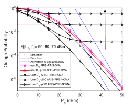
Fig. 2: Outage probability versus the transmitting power of the BS for PRIS-ARIS-NOMA.

Fig. 3 depicts the outage probability for the comparison of PRIS-ARIS-NOMA and double PRISs-NOMA versus the total power consumption of the networks with settings of $\Omega_{RI}=-80$ dBm. In this case, the outage probability of users without RISs assistance scenario is also plotted in the figure, and it can be seen that the user outage performance of the communication link without RISs assistance is poor in this communication environment. As can be observed from the figure that the outage performance of PRIS-ARIS networks is better than the double PRISs networks, the cause of this phenomenon is that ARIS is equipped with active bias circuitry compared to PRIS and has a built-in signal amplifier to increase the signal power, which helps improve the user’s reception SNR at the receiving end. It also reflects that the use of ARIS can better combat fading in the channel with the comparison to PRIS.

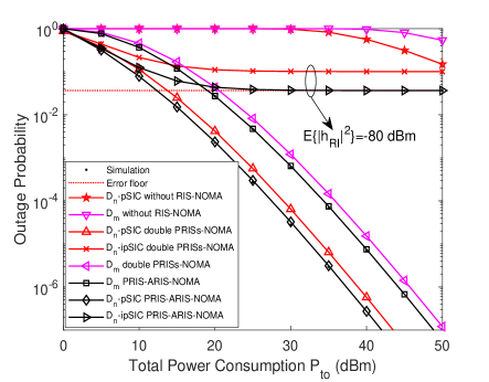
Fig. 3: Outage probability versus the total power consumption.

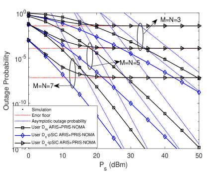
Fig. 4: Outage probability versus the transmitting power of the BS for PRIS-ARIS-NOMA.

Fig. 4 depicts the outage probability of PRIS-ARIS-NOMA versus the transmitting power of the BS with settings of $\Omega_{RI}=-80$ dBm, and compares users outage probability with different reflecting elements. From the trend of outage probability in the figure, we can find that as the number of RISs reflecting elements increases, the users will tend to get a better outage performance. This is because that the number of reflecting elements determines the number of independent divisions of the transmission, and as the number of independent divisions increases, the ability of the signal to fight against channel fading increases by a certain degree, so the users outage performance becomes better. Meanwhile, in line with Remark 2 and Remark 3, the diversity orders of $D_{n}$ and $D_{m}$ are affected by the reflecting elements on RISs. Therefore, as the number of reflecting elements $M$ increases, the users outage probability curves gain a larger slope and decrease faster.

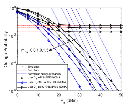
Fig. 5: Outage probability versus the transmitting power of the BS for PRIS-ARIS-NOMA.

Fig. 5 depicts the outage probability of PRIS-ARIS-NOMA versus the transmitting power of the BS with settings of $\Omega_{RI}=-80$ dBm, and compares users outage probability with different shaping parameter $m_{na}$ of Nakagami-$m$ random variables. From the figure, it can be intuitively observed that the outage performance of users gradually becomes better as $m_{na}$ increases. This is because the physical meaning of $m_{na}$ in the communication scenario represents the depth of channel fading, with larger $m_{na}$ indicating shallower channel fading and higher communication quality of the communication channels. Theoretically, when $m_{na}$ tends to 0, it means communication is almost impossible to achieve, and when $m_{na}$ tends to infinity, it means no fading exists in the communication channels. It can also be observed from the figure that the variation of $m_{na}$ does not affect the slope of the users outage probability, which is due to the fact that the user’s diversity order depends only on the reflecting elements number of ARIS, which coincides with the Remark 2 and Remark 3.

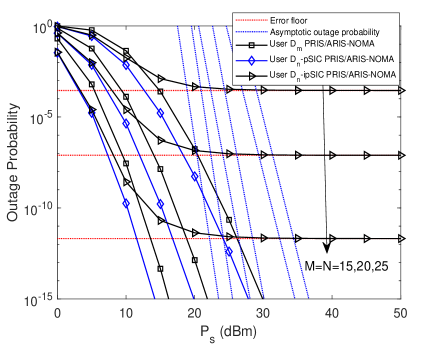
Fig. 6: Outage probability versus the transmitting power of the BS for PRIS-ARIS-NOMA over long-distance transmission scenario.

In order to demonstrate the advantages of this system model for long-distance transmission, we also analyzed a scenario of PRIS-ARIS-NOMA networks for long-distance transmission as shown in Fig. 6. In this scenario, the distance between the communication links is set as $d_{h1}=d_{h2}=d_{g1}=1000{\text{ m}}$, $d_{gn}=800{\text{ m}}$, $d_{gm}=1800{\text{ m}}$ respectively, and the number of reflecting elements used by the two RISs grows moderately as well. From the figure, it can be seen that the PRIS-ARIS-NOMA networks has a significant enhancement of the communication performance for long-distance transmission, and the users outage probabilities can reach a threshold of $10^{-3}$ at a transmitting power around 5 dBm. Also as the number of reflecting elements increases, the outage probability decreases more rapidly, which confirms the insights obtained from the Remark 2 and Remark 3.

V-B Ergodic Data Rate

Fig. 7 depicts the ergodic data rate of PRIS-ARIS-NOMA versus the transmitting power of the BS with settings of $\Omega_{RI}=-80$ dBm, and also compares the ergodic data rate of $D_{n}$ and $D_{m}$ under OMA networks. As shown in the figure, the curves of ergodic data rate for $D_{n}$ with ipSIC/pSIC and $D_{m}$ can be plotted in terms of (4), (5) and (5), while the curves of ergodic rate for user $D_{n}$ and user $D_{m}$ under OMA networks can be plotted in terms of (6). And the curves for asymptotic ergodic data rate can be plotted in terms of (32), (IV-D2) and (IV-D3). The figure shows that the ergodic data rate of $D_{n}$ with ipSIC and $D_{m}$ eventually converge to an upper throughput limit and converge to a zero ergodic data rate slope at high SNR region, which are in lines with the Remark 4 and Remark 6. This is because for $D_{n}$ with ipSIC, it is similar to the analysis of the outage probability, self interference affects the users receiving performance more as the transmitting power increases. And for $D_{m}$, upper throughput limit is only dependent on the power allocation factors of the two users according to (IV-D3). Moreover, the ergodic performance of $D_{n}$ with ipSIC under NOMA networks is better than that of the OMA networks. For OMA networks, the division of resources for per user in the frequency domain is reduced by one-half compared to NOMA systems, so the ergodic data rate slope of the OMA networks is reduced by one-half compared to NOMA networks, which is the reason why the ergodic data rate under OMA networks grows slower than that of the NOMA networks.

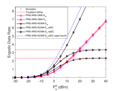
Fig. 7: Ergodic data rate versus the transmitting power of the BS for PRIS-ARIS-NOMA.

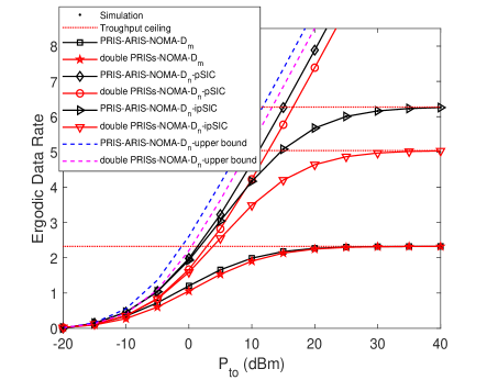
Fig. 8: Ergodic data rate versus the total power consumption.

Fig. 8 depicts the ergodic data rate for the comparison of PRIS-ARIS-NOMA and double PRISs-NOMA versus the total power consumption of the networks with settings of $\Omega_{RI}=-80$ dBm. One can be seen is that the ergodic data rates of $D_{n}$ with ipSIC/pSIC and $D_{m}$ in PRIS-ARIS-NOMA are superior to that in double PRISs-NOMA, this is because that ARIS amplifies and forwards the signals through the built-in bias circuit, which can increase the SINR at the receiving end, so the ergodic data rate will be higher. Fig. 9 depicts the ergodic data rate for PRIS-ARIS-NOMA versus the transmitting power of the BS with settings of $\Omega_{RI}=-80$ dBm, and compares the ergodic data rate of the two users under different number of reflecting elements of the ARIS. From the figure we can observe that as the number of ARIS reflecting elements increases, the ergodic data rate gradually increases.

Fig. 9: Ergodic data rate versus the transmitting power of the BS for PRIS-ARIS-NOMA.

V-C System Throughput

Fig. 10: System throughput versus the total power consumption.

Fig. 10 depicts the system throughput for the comparison of PRIS-ARIS-NOMA and double PRISs-NOMA versus the total power consumption of the networks in delay-limited transmission mode with settings of $\Omega_{RI}=-80$ dBm. The curves for the system throughput in delay-limited transmission mode can be drawn in terms of (25). It can be observed from the figure that the system throughput of the PRIS-ARIS-NOMA in delay-limited transmission mode is higher than that of the double PRISs networks and OMA networks. This is due to the fact that the system throughput in delay-limited transmission mode is relevant to the system outage probability and a lower outage probability yields a higher throughput. Another phenomenon is that the system throughput with ipSIC scheme cannot reach the maximum value. This is because residual interference limits the extent to which the outage probability decreases with increasing transmitting power, thus producing an upper limit on the system throughput that does not reach the expected maximum value.

Fig. 11: System throughput versus the transmitting power of the BS for PRIS-ARIS-NOMA.

Fig. 11 depicts the the system throughput for PRIS-ARIS-NOMA versus the transmitting power of the BS in delay-tolerant transmission mode with settings of $\Omega_{RI}=-80$ dBm. The curves for the system throughput in delay-tolerant transmission mode can be drawn in terms of (35). From the figure, we can observe that the throughput of the system can be improved by increasing the number of RIS reflecting elements and reducing the power of self interference under the ipSIC scheme. It also reflects the importance of optimizing the SIC process in NOMA networks.

VI Conclusion

In this paper, the PRIS-ARIS assisted NOMA networks under cascaded Rician fading and Nakagami-$m$ fading channels have been studied in detail. Specifically, the closed-form expressions for outage probability and ergodic data rate of a pair of two non-orthogonal users have been derived in detail, as well as the asymptotic expressions for outage probability and ergodic data rate are deduced for more insights. Moreover, diversity orders and ergodic data rate slopes are analyzed based on the asymptotic expression to evaluate the performance of the networks. Furthermore, the system throughput in delay-limited mode and delay-tolerant mode are evaluated to show the system enhancement. Eventually, through detailed study of this paper, we can find that PRIS-ARIS-NOMA outperforms PRIS-ARIS-OMA and double PRISs-NOMA. Compared to PRIS, the use of ARIS at user end can better combat channel fading under the cascaded channel scenario. And as the number of RISs reflecting elements increases within a certain range, the networks tend to perform better.

Appendix A: Proof of Theorem 1

To prove this theorem, we started by bringing (2) and (4) into (12). The outage probability expression of $D_{n}$ with ipSIC can be further derived as (Appendix A: Proof of Theorem 1) at the top of the next page. Then, simplifying (Appendix A: Proof of Theorem 1) yields

$$P_{{D_{n}}}^{ipSIC}= \Pr\left({\frac{{\beta{P_{s}^{a}}{{\left|{{\mathbf{h}}_{2}^{T}{{\mathbf{\Phi}}_{p}}{{\mathbf{h}}_{1}}}\right|}^{2}}{{\left|{{\mathbf{g}}_{n}^{T}{{\mathbf{\Phi}}_{a}}{{\mathbf{g}}_{1}}}\right|}^{2}}{a_{m}}}}{{\beta{P_{s}^{a}}{{\left|{{\mathbf{h}}_{2}^{T}{{\mathbf{\Phi}}_{p}}{{\mathbf{h}}_{1}}}\right|}^{2}}{{\left|{{\mathbf{g}}_{n}^{T}{{\mathbf{\Phi}}_{a}}{{\mathbf{g}}_{1}}}\right|}^{2}}{a_{n}}+\beta\sigma_{a}^{2}{{\left\|{{\mathbf{g}}_{n}^{T}{{\mathbf{\Phi}}_{a}}}\right\|}^{2}}+{\sigma^{2}}}}<{\gamma_{t{h_{m}}}}}\right)\hfill$$

$$+\Pr\left({\frac{{\beta{P_{s}^{a}}{{\left|{{\mathbf{h}}_{2}^{T}{{\mathbf{\Phi}}_{p}}{{\mathbf{h}}_{1}}}\right|}^{2}}{{\left|{{\mathbf{g}}_{n}^{T}{{\mathbf{\Phi}}_{a}}{{\mathbf{g}}_{1}}}\right|}^{2}}{a_{m}}}}{{\beta{P_{s}^{a}}{{\left|{{\mathbf{h}}_{2}^{T}{{\mathbf{\Phi}}_{p}}{{\mathbf{h}}_{1}}}\right|}^{2}}{{\left|{{\mathbf{g}}_{n}^{T}{{\mathbf{\Phi}}_{a}}{{\mathbf{g}}_{1}}}\right|}^{2}}{a_{n}}+\beta\sigma_{a}^{2}{{\left\|{{\mathbf{g}}_{n}^{T}{{\mathbf{\Phi}}_{a}}}\right\|}^{2}}+{\sigma^{2}}}}>{\gamma_{t{h_{m}}}},\frac{{\beta{P_{s}^{a}}{{\left|{{\mathbf{h}}_{2}^{T}{{\mathbf{\Phi}}_{p}}{{\mathbf{h}}_{1}}}\right|}^{2}}{{\left|{{\mathbf{g}}_{n}^{T}{{\mathbf{\Phi}}_{a}}{{\mathbf{g}}_{1}}}\right|}^{2}}{a_{n}}}}{{\varpi{P_{s}^{a}}{{\left|{{h_{RI}}}\right|}^{2}}+\beta\sigma_{a}^{2}{{\left\|{{\mathbf{g}}_{n}^{T}{{\mathbf{\Phi}}_{a}}}\right\|}^{2}}+{\sigma^{2}}}}<{\gamma_{t{h_{n}}}}}\right).$$ (A.1)

$$P_{{D_{n}}}^{out,ipSIC} =\Pr\left[{\underbrace{{{\left|{\sum\limits_{n=0}^{N}{h_{n}^{1}}h_{n}^{2}}\right|}^{2}}}_{{\zeta_{h}}}\underbrace{{{\left|{\sum\limits_{m=0}^{M}{g_{m}^{1}}g_{m}^{\varphi}}\right|}^{2}}}_{{\zeta_{g}}}}\right.\hfill$$

$$\left.{<\frac{{\overline{{\lambda_{n}}}{\gamma_{t{h_{n}}}}\left({\varpi{P_{s}^{a}}{{\left|{{h_{RI}}}\right|}^{2}}+\beta\sigma_{a}^{2}{{\left\|{{\mathbf{g}}_{n}^{T}{{\mathbf{\Phi}}_{a}}}\right\|}^{2}}+{\sigma^{2}}}\right)}}{{\beta{P_{s}^{a}}{a_{n}}}}}\right],$$ (A.2)

where, $\overline{{\lambda_{n}}}={\eta^{-4}}d_{h1}^{\alpha}d_{h2}^{\alpha}d_{g1}^{\alpha}d_{gn}^{\alpha}$, and the PDF of $\zeta_{h}$ and $\zeta_{g}$ are denoted by (10) and (11) in Section II. The operation here needs to obtain the PDF of ${\zeta_{h}}{\zeta_{g}}$, and combine (10) and (11), the PDF of $Z={\zeta_{h}}{\zeta_{g}}$ can be derived by

$${F_{Z}}\left(z\right) =\int_{0}^{\infty}{\left[{\int_{0}^{\frac{z}{x}}{{f_{{\zeta_{g}}}}\left(y\right)}dy}\right]}{f_{{\zeta_{h}}}}\left(x\right)dx.$$ (A.3)

Performing a mathematical simplification and using Gauss-Laguerre quadrature formula [52, Sec. 2.2.2] to approximate the result of the integral expression yields

$${F_{Z}}\left(z\right)=\sum\limits_{u=1}^{U}{\frac{{{H_{u}}x_{u}^{{a_{X}}}}}{{\Gamma({a_{X}}+1)\Gamma({a_{Y}}+1)}}\gamma\left({{a_{Y}}+1,\frac{{\sqrt{z}}}{{{b_{X}}{b_{Y}}{x_{u}}}}}\right)},$$ (A.4)

where $\gamma(\alpha,x)=\int_{0}^{x}{{e^{-t}}{t^{\alpha-1}}}dt$ means the lower incomplete gamma function[51, Eq. (8.350.1)]. ${{H_{u}}}$ and $x_{u}$ are the $u$-th weight and $u$-th zero point of Laguerre polynomial ${L_{u}}({x_{u}})$, respectively. Specifically, ${H_{u}}=\frac{{{{[(U+1)!]}^{2}}}}{{{x_{u}}{{[{{L^{\prime}}_{U+1}}({x_{u}})]}^{2}}}},u=0,1,...,U$ and ${L_{\varphi}}\left(x\right)={e^{x}}\frac{{{d^{\varphi}}}}{{d{x^{\varphi}}}}\left({{x^{\varphi}}{e^{-x}}}\right)$.

In (Appendix A: Proof of Theorem 1), the self interference part ${{{\left|{{h_{RI}}}\right|}^{2}}}$ follows an exponential distribution with parameter ${\Omega_{RI}}$. Then, by substituting (A.4) into (Appendix A: Proof of Theorem 1) and approximating thermal noise part ${{\left\|{{\mathbf{g}}_{n}^{T}{{\mathbf{\Phi}}_{a}}}\right\|}^{2}}$ to ${M{\Omega_{na}}}$, the expression of outage probability for $D_{n}$ with ipSIC can be derived by

$$P_{{D_{n}}}^{out,ipSIC} =\int_{0}^{+\infty}{\frac{1}{{{\Omega_{RI}}}}{e^{-\frac{x}{{{\Omega_{RI}}}}}}}\hfill$$

$$\times{F_{Z}}\left[{\frac{{\overline{{\lambda_{n}}}{\gamma_{t{h_{n}}}}\left({\varpi{P_{s}^{a}}x+\beta\sigma_{a}^{2}M{\Omega_{na}}+{\sigma^{2}}}\right)}}{{\beta{P_{s}^{a}}{a_{n}}}}}\right]dx.$$ (A.5)

Finally, by once again using the Gauss-Laguerre quadrature formula in (Appendix A: Proof of Theorem 1) and performing algebraic operations, (1) can be obtained. The proof is completed.

Appendix B: Proof of Corollary 3

Proof starts with substituting $\varpi=0$ into (Appendix A: Proof of Theorem 1) and the outage probability of $D_{n}$ with pSIC can be expressed as

$$P_{{D_{n}}}^{out,pSIC}= \Pr\left[{\underbrace{\left({\sum\limits_{n=0}^{N}{\left|{h_{n}^{1}h_{n}^{2}}\right|}}\right)}_{{{\hat{\zeta}}_{h}}}\underbrace{\left({\sum\limits_{m=0}^{M}{\left|{g_{m}^{1}g_{m}^{\varphi}}\right|}}\right)}_{{{\hat{\zeta}}_{g}}}}\right.\hfill$$

$$\left.{<\sqrt{\frac{{\overline{{\lambda_{n}}}{\gamma_{t{h_{n}}}}\left({\beta\sigma_{a}^{2}{{\left\|{{\mathbf{g}}_{n}^{T}{{\mathbf{\Phi}}_{a}}}\right\|}^{2}}+{\sigma^{2}}}\right)}}{{\beta{P_{s}^{a}}{a_{n}}}}}}\right].$$ (B.1)

Then to derive the expression of the asymptotic outage probability, the next step is to obtain the approximate CDF expression of $\hat{Z}={{\hat{\zeta}}_{h}}{{\hat{\zeta}}_{g}}$ at high SNR region. Using the Laplace transform on (II-B) with the help of the integral formula [52, Sec. 6.621.3] yields

$$\mathcal{L} \left[{{f_{{X_{n}}}}\left(y\right)}\right]\left(s\right)=\sum\limits_{m=0}^{\infty}{\frac{{4{\kappa^{m}}{{\left[{\left({\kappa+1}\right){m_{na}}}\right]}^{\frac{1}{2}\left({1+m+{m_{na}}}\right)}}}}{{{e^{\kappa}}{{\left({m!}\right)}^{2}}\Gamma\left({{m_{na}}}\right)}}}\hfill$$

$$\times\frac{{\sqrt{\pi}{{\left({4\sqrt{\left({\kappa+1}\right){m_{na}}}}\right)}^{m-{m_{na}}+1}}}}{{{{\left({s+2\sqrt{\left({\kappa+1}\right){m_{na}}}}\right)}^{2m+2}}}}\frac{{\Gamma\left({2m+2}\right)\Gamma\left({2{m_{na}}}\right)}}{{\Gamma\left({m+{m_{na}}+\frac{3}{2}}\right)}}\hfill$$

$$\times F\left({2m+2,m-{m_{na}}+\frac{3}{2};m+{m_{na}}+\frac{3}{2};{\Upsilon_{s}}}\right),$$ (B.2)

where ${\Upsilon_{s}}=\frac{{s-2\sqrt{\left({\kappa+1}\right){m_{na}}}}}{{s+2\sqrt{\left({\kappa+1}\right){m_{na}}}}}$. When ${{P_{s}}\to\infty}$ in the time domain, $s$ tends to infinity in the complex frequency domain simultaneously. Therefore, $\frac{{s-2\sqrt{\left({\kappa+1}\right){m_{na}}}}}{{s+2\sqrt{\left({\kappa+1}\right){m_{na}}}}}$ can be approximated to 1 and $s+2\sqrt{\left({\kappa+1}\right){m_{na}}}$ can be approximated as $s$. Letting $\Delta\left(m\right)$ as

$$\Delta\left(m\right) =\frac{{{\kappa^{m}}{{\left[{\left({\kappa+1}\right){m_{na}}}\right]}^{\frac{1}{2}\left({1+m+{m_{na}}}\right)}}}}{{{{\left({m!}\right)}^{2}}\Gamma\left({m+{m_{na}}+\frac{3}{2}}\right)}}\hfill$$

$$\times{\left({4\sqrt{\left({\kappa+1}\right){m_{na}}}}\right)^{m-{m_{na}}+1}}\Gamma\left({2m+2}\right)\hfill$$

$$\times F\left({2m+2,m-{m_{na}}+\frac{3}{2};m+{m_{na}}+\frac{3}{2};1}\right),$$ (B.3)

the Laplace transform of ${X_{n}}=\left|{h_{n}^{1}h_{n}^{2}}\right|$ can be eventually derived as

$$\mathcal{L}\left[{{f_{{X_{n}}}}\left(y\right)}\right]\left(s\right)=\sum\limits_{m=0}^{\infty}{\frac{{4\sqrt{\pi}\Gamma\left({2{m_{na}}}\right)\Delta\left(m\right)}}{{{e^{\kappa}}\Gamma\left({{m_{na}}}\right)}}}\frac{1}{{{s^{2m+2}}}}.$$ (B.4)

As a further advance, based on (B.4) and then using the convolution theorem, the Laplace transform of the PDF of ${{{\hat{\zeta}}_{h}}}$ can be given by

$$\mathcal{L}\left[{{f_{{{\hat{\zeta}}_{h}}}}\left(y\right)}\right]\left(s\right)={\left[{\sum\limits_{m=0}^{\infty}{\frac{{4\sqrt{\pi}\Gamma\left({2{m_{na}}}\right)\Delta\left(m\right)}}{{{e^{\kappa}}\Gamma\left({{m_{na}}}\right)}}}\frac{1}{{{s^{2m+2}}}}}\right]^{N}}.$$ (B.5)

The first term of the series is taken i.e.,$m=0$, and then appling inverse Laplace transform to (B.5), the PDF of ${{{\hat{\zeta}}_{h}}}$ at high SNR region can be derived as

$${f_{{{\hat{\zeta}}_{h}}}}\left(y\right)={\left[{\frac{{4\sqrt{\pi}\Gamma\left({2{m_{na}}}\right)\Delta\left(0\right)}}{{{e^{\kappa}}\Gamma\left({{m_{na}}}\right)}}}\right]^{N}}\frac{{{y^{2N-1}}}}{{\left({2N-1}\right)!}}.$$ (B.6)

Similarly, the derivation of ${{{\hat{\zeta}}_{g}}}$ follows the same process as above. Referring to the process of (A.3) and using the transformation of the Gaussian Chebyshev quadrature formula[56, Eq. (8.8.12)], the CDF expression for $\hat{Z}={{\hat{\zeta}}_{h}}{{\hat{\zeta}}_{g}}$ at high SNR region can be obtained as

$${F_{\hat{Z}}}\left(z\right) =\frac{{\pi{\mu_{b}}{z^{2M}}}}{{2K\left({2M}\right)!\left({2N-1}\right)!}}{\left[{\frac{{4\sqrt{\pi}\Gamma\left({2{m_{na}}}\right)\Delta\left(0\right)}}{{{e^{\kappa}}\Gamma\left({{m_{na}}}\right)}}}\right]^{M+N}}\hfill$$

$$\times\sum\limits_{k=1}^{K}{{{\left[{\frac{{\left({{x_{k}}{\text{ + }}1}\right){\mu_{b}}}}{2}}\right]}^{2N-2M-1}}\sqrt{1-{x_{k}}^{2}}},$$ (B.7)

where $K$ is the parameter of the Gauss-Chebyshev quadrature formula for precision. $\mu_{b}$ is the upper limit of integral before using the Gauss-Chebyshev quadrature formula for the approximation and ${\mu_{b}}\to\infty$. ${x_{k}}=\cos\left({\frac{{2k-1}}{{2K}}\pi}\right)$.

Finally, by submitting (Appendix B: Proof of Corollary 3) into (Appendix B: Proof of Corollary 3), (22) can be obtained. The proof is completed.

Appendix C: Proof of Theorem 4

The proof starts by substituting (3) into (26) and we can obtain the expression of ergodic data rate for $D_{n}$ with ipSIC as

$$R_{Dn,ipSIC}^{ergodic}=\mathbb{E}\left[{{{\log}_{2}}\left({1+\frac{{\beta{P_{s}^{a}}{{\left|{{\mathbf{h}}_{2}^{T}{{\mathbf{\Phi}}_{p}}{{\mathbf{h}}_{1}}}\right|}^{2}}{{\left|{{\mathbf{g}}_{n}^{T}{{\mathbf{\Phi}}_{a}}{{\mathbf{g}}_{1}}}\right|}^{2}}{a_{n}}}}{{\varpi{P_{s}^{a}}\sigma_{ri}^{2}+\beta\sigma_{a}^{2}{{\left\|{{\mathbf{g}}_{n}^{T}{{\mathbf{\Phi}}_{a}}}\right\|}^{2}}+{\sigma^{2}}}}}\right)}\right].$$ (C.1)

By referring to the process of proving the outage probability of $D_{n}$ with ipSIC in Appendix A and with the use of (1), we can obtain the CDF of $\gamma_{{D_{n}}}$ as

$${F_{{\gamma_{{D_{n}}}}}}\left(z\right)=\sum\limits_{i=1}^{I}{\sum\limits_{u=1}^{U}{\frac{{{H_{i}}{H_{u}}x_{u}^{{a_{X}}}}}{{\Gamma({a_{X}}+1)\Gamma({a_{Y}}+1)}}}}\hfill$$

$$\times\gamma\left({{a_{Y}}+1,\frac{{\sqrt{z{{\bar{\lambda}}_{n}}\left({{P_{s}^{a}}{\Omega_{RI}}{x_{i}}+\beta\sigma_{a}^{2}M{\Omega_{na}}+{\sigma^{2}}}\right)}}}{{\sqrt{\beta{P_{s}^{a}}{a_{n}}}{b_{X}}{b_{Y}}{x_{u}}}}}\right).$$ (C.2)

With the help of the definition expression for the lower incomplete Gamma function, we can obtain the PDF of $\gamma_{{D_{n}}}$ on the basis of (Appendix C: Proof of Theorem 4) as

$${f_{{\gamma_{{D_{n}}}}}}\left(z\right)=\sum\limits_{i=1}^{I}{\sum\limits_{u=1}^{U}{\frac{{{a^{{a_{Y}}+1}}{H_{i}}{H_{u}}x_{u}^{{a_{X}}}{z^{\frac{{{a_{Y}}}}{2}}}{e^{-\chi\sqrt{z}}}}}{{2\sqrt{z}\Gamma({a_{X}}+1)\Gamma({a_{Y}}+1)}}}},$$ (C.3)

where $\chi=\frac{{\sqrt{z{{\bar{\lambda}}_{n}}\left({{P_{s}}{\Omega_{RI}}{x_{i}}+\beta\sigma_{a}^{2}M{\Omega_{na}}+{\sigma^{2}}}\right)}}}{{\sqrt{\beta{P_{s}}{a_{n}}}{b_{X}}{b_{Y}}{x_{u}}}}$.

Combining (C.1) and (C.3), the ergodic data rate of $D_{n}$ with ipSIC for PRIS-ARIS-NOMA can be given by

$$R_{n}^{ergodic}=\frac{1}{{\ln 2}}\int_{0}^{+\infty}{\ln\left({1+y}\right){f_{{\gamma_{{D_{n}}}}}}\left(y\right)}dy\hfill$$

$$=\frac{1}{{\ln 2}}\int_{0}^{+\infty}{\ln\left({1+y}\right)}\sum\limits_{i=1}^{I}{\sum\limits_{u=1}^{U}{\frac{{{a^{{a_{Y}}+1}}{H_{i}}{H_{u}}x_{u}^{{a_{X}}}{z^{\frac{{{a_{Y}}}}{2}}}{e^{-\chi\sqrt{z}}}}}{{2\sqrt{z}\Gamma({a_{X}}+1)\Gamma({a_{Y}}+1)}}}}dy.$$ (C.4)

Finally, by bringing into Gauss-Laguerre quadrature, (4) can be obtained. The proof is completed.

Appendix D: Proof of Theorem 6

The proof starts similarly to the (C.1) by substituting (4) into (26) and we can obtain the expression of ergodic data rate for $D_{m}$ as

$$R_{{D_{m}}}^{ergodic} =\mathbb{E}\left[{{{\log}_{2}}\left({1+}\right.}\right.\hfill$$

$$\left.{\left.{\frac{{\beta{P_{s}^{a}}{{\left|{{\mathbf{h}}_{2}^{T}{{\mathbf{\Phi}}_{p}}{{\mathbf{h}}_{1}}}\right|}^{2}}{{\left|{{\mathbf{g}}_{m}^{T}{{\mathbf{\Phi}}_{a}}{{\mathbf{g}}_{1}}}\right|}^{2}}{a_{m}}}}{{\beta{P_{s}^{a}}{{\left|{{\mathbf{h}}_{2}^{T}{{\mathbf{\Phi}}_{p}}{{\mathbf{h}}_{1}}}\right|}^{2}}{{\left|{{\mathbf{g}}_{m}^{T}{{\mathbf{\Phi}}_{a}}{{\mathbf{g}}_{1}}}\right|}^{2}}{a_{n}}+\beta\sigma_{a}^{2}{{\left\|{{\mathbf{g}}_{n}^{T}{{\mathbf{\Phi}}_{a}}}\right\|}^{2}}+{\sigma^{2}}}}}\right)}\right].$$ (D.1)

By referring to the process of proving the outage probability of $D_{m}$ and with the use of (2), we can obtain the CDF of $\gamma_{{D_{m}}}$ as

$${F_{{{\gamma_{{D_{m}}}}}}}\left(x\right)= \sum\limits_{u=1}^{U}{\frac{{x_{u}^{{a_{X}}}{H_{u}}}}{{\Gamma({a_{X}}+1)\Gamma({a_{Y}}+1)}}}\hfill$$

$$\times\gamma\left({{a_{Y}}+1,\frac{{\sqrt{\overline{{\lambda_{m}}}x\left({\beta\sigma_{a}^{2}M{\Omega_{na}}+{\sigma^{2}}}\right)}}}{{\sqrt{\beta{P_{s}^{a}}\left({{a_{m}}-x{a_{n}}}\right)}{b_{X}}{b_{Y}}{x_{u}}}}}\right),$$ (D.2)

it should be noted that in order to ensure the correctness of the calculation, it is necessary here to satisfy $x<\frac{{{a_{m}}}}{{{a_{n}}}}$, which is different from the process of solving for (Appendix C: Proof of Theorem 4). Combining (Appendix D: Proof of Theorem 6) and (Appendix D: Proof of Theorem 6), the ergodic data rate of $D_{m}$ for PRIS/ARIS-NOMA can be given by

$$R_{m}^{ergodic}= \frac{1}{{\ln 2}}\int_{0}^{\frac{{{a_{m}}}}{{{a_{n}}}}}{\frac{{1-{F_{{\gamma_{{D_{m}}}}}}\left(x\right)}}{{1+x}}dx},$$ (D.3)

Finally, by bringing into the transformation of the Gaussian Chebyshev quadrature formula, (5) can be obtained. The proof is completed.

References

- [1] A. Gupta and R. K. Jha, “A survey of 5G network: Architecture and emerging technologies,” IEEE Access, vol. 3, pp. 1206–1232, Jul. 2015.
- [2] X. Wang, J. Mei, S. Cui, C.-X. Wang, and X. S. Shen, “Realizing 6G: The operational goals, enabling technologies of future networks, and value-oriented intelligent multi-dimensional multiple access,” IEEE Netw., vol. 37, no. 1, pp. 10–17, Feb. 2023.
- [3] L. Dai, B. Wang, M. Wang, X. Yang, J. Tan, S. Bi, S. Xu, F. Yang, Z. Chen, M. D. Renzo, C.-B. Chae, and L. Hanzo, “Reconfigurable intelligent surface-based wireless communications: Antenna design, prototyping, and experimental results,” IEEE Access, vol. 8, pp. 45 913–45 923, Mar. 2020.
- [4] E. Basar and H. V. Poor, “Present and future of reconfigurable intelligent surface-empowered communications [perspectives],” IEEE Signal Process. Mag., vol. 38, no. 6, pp. 146–152, Nov. 2021.
- [5] C. Pan, H. Ren, K. Wang, J. F. Kolb, M. Elkashlan, M. Chen, M. Di Renzo, Y. Hao, J. Wang, A. L. Swindlehurst, X. You, and L. Hanzo, “Reconfigurable intelligent surfaces for 6G systems: Principles, applications, and research directions,” IEEE Commun. Mag., vol. 59, no. 6, pp. 14–20, Jun. 2021.
- [6] Y. Liu, X. Liu, X. Mu, T. Hou, J. Xu, M. Di Renzo, and N. Al-Dhahir, “Reconfigurable intelligent surfaces: Principles and opportunities,” IEEE Commun. Surveys Tuts, vol. 23, no. 3, pp. 1546–1577, May 2021.
- [7] S. Hu, F. Rusek, and O. Edfors, “Beyond massive MIMO: The potential of data transmission with large intelligent surfaces,” IEEE Trans. Sig. Proc., vol. 66, no. 10, pp. 2746–2758, May 2018.
- [8] Z. Zhang and L. Dai, “Reconfigurable intelligent surfaces for 6G: Nine fundamental issues and one critical problem,” Tsinghua Sci. Technol., vol. 28, no. 5, pp. 929–939, Oct. 2023.
- [9] A. L. Swindlehurst, G. Zhou, R. Liu, C. Pan, and M. Li, “Channel estimation with reconfigurable intelligent surfaces - A general framework,” Proc. IEEE, vol. 110, no. 9, pp. 1312–1338, Sep. 2022.
- [10] M. Di Renzo, F. H. Danufane, and S. Tretyakov, “Communication models for reconfigurable intelligent surfaces: From surface electromagnetics to wireless networks optimization,” Proc. IEEE, vol. 110, no. 9, pp. 1164–1209, Sep. 2022.
- [11] H. Zhang, B. Di, Z. Han, H. V. Poor, and L. Song, “Reconfigurable intelligent surface assisted multi-user communications: How many reflective elements do we need?” IEEE Wireless Commun. Lett., vol. 10, no. 5, pp. 1098–1102, May 2021.
- [12] T. Van Chien, A. K. Papazafeiropoulos, L. T. Tu, R. Chopra, S. Chatzinotas, and B. Ottersten, “Outage probability analysis of IRS-assisted systems under spatially correlated channels,” IEEE Wireless Commun. Lett., vol. 10, no. 8, pp. 1815–1819, Aug. 2021.
- [13] N. Mensi and D. B. Rawat, “Reconfigurable intelligent surface selection for wireless vehicular communications,” IEEE Wireless Commun. Lett., vol. 11, no. 8, pp. 1743–1747, Aug. 2022.
- [14] Q. Tao, J. Wang, and C. Zhong, “Performance analysis of intelligent reflecting surface aided communication systems,” IEEE Commun. Lett., vol. 24, no. 11, pp. 2464–2468, Nov. 2020.
- [15] M. H. Khoshafa, T. M. N. Ngatched, M. H. Ahmed, and A. R. Ndjiongue, “Active reconfigurable intelligent surfaces-aided wireless communication system,” IEEE Commun. Lett., vol. 25, no. 11, pp. 3699–3703, Nov. 2021.
- [16] R. Long, Y.-C. Liang, Y. Pei, and E. G. Larsson, “Active reconfigurable intelligent surface-aided wireless communications,” IEEE Trans. Wireless Commun., vol. 20, no. 8, pp. 4962–4975, Aug. 2021.
- [17] Z. Zhang, L. Dai, X. Chen, C. Liu, F. Yang, R. Schober, and H. V. Poor, “Active RIS vs. passive RIS: Which will prevail in 6G?” IEEE Trans. Commun., vol. 71, no. 3, pp. 1707–1725, Mar. 2023.
- [18] K. Liu, Z. Zhang, L. Dai, S. Xu, and F. Yang, “Active reconfigurable intelligent surface: Fully-connected or sub-connected?” IEEE Commun. Lett., vol. 26, no. 1, pp. 167–171, Jan. 2022.
- [19] C. You and R. Zhang, “Wireless communication aided by intelligent reflecting surface: Active or Passive?” IEEE Wireless Commun. Lett., vol. 10, no. 12, pp. 2659–2663, Dec. 2021.
- [20] X. Yue, M. Song, C. Ouyang, Y. Liu, T. Li, and T. Hou, “Exploiting active RIS in NOMA networks with hardware impairments,” IEEE Trans. Veh. Technol., pp. 1–16, Jun. 2024.
- [21] Y. Wang, W. Zhang, Y. Chen, C.-X. Wang, and J. Sun, “Novel multiple RIS-assisted communications for 6G networks,” IEEE Commun. Lett., vol. 26, no. 6, pp. 1413–1417, Jun. 2022.
- [22] Q. Sun, P. Qian, W. Duan, J. Zhang, J. Wang, and K.-K. Wong, “Ergodic rate analysis and IRS configuration for multi-IRS dual-hop df relaying systems,” IEEE Commun. Lett., vol. 25, no. 10, pp. 3224–3228, Oct. 2021.
- [23] Y. Zhang, C. You, and B. Zheng, “Multi-active multi-passive (MAMP)-IRS aided wireless communication: A multi-hop beam routing design,” IEEE J. Sel. Areas Commun., pp. 1–1, Aug. 2023.
- [24] B. Zheng, C. You, and R. Zhang, “Double-IRS assisted multi-user MIMO: Cooperative passive beamforming design,” IEEE Trans. Wireless Commun., vol. 20, no. 7, pp. 4513–4526, Jul. 2021.
- [25] Y. Liu, X. Mu, J. Xu, R. Schober, Y. Hao, H. V. Poor, and L. Hanzo, “STAR: Simultaneous transmission and reflection for 360 coverage by intelligent surfaces,” IEEE Wirel. Communi., vol. 28, no. 6, pp. 102–109, Dec. 2021.
- [26] J. Xu, Y. Liu, X. Mu, and O. A. Dobre, “STAR-RISs: Simultaneous transmitting and reflecting reconfigurable intelligent surfaces,” IEEE Communi. Lett., vol. 25, no. 9, pp. 3134–3138, Sep. 2021.
- [27] Y. Liu, Z. Qin, M. Elkashlan, Z. Ding, A. Nallanathan, and L. Hanzo, “Non-orthogonal multiple access for 5G and beyond,” Proceedings of the IEEE, vol. 105, no. 12, pp. 2347–2381, Oct. 2017.
- [28] X. Liu, B. Lin, M. Zhou, and M. Jia, “NOMA-based cognitive spectrum access for 5G-enabled Internet of Things,” IEEE Netw., vol. 35, no. 5, pp. 290–297, Sept. 2021.
- [29] X. Pei, Y. Chen, M. Wen, H. Yu, E. Panayirci, and H. V. Poor, “Next-generation multiple access based on NOMA with power level modulation,” IEEE J. Sel. Areas Commun., vol. 40, no. 4, pp. 1072–1083, Apr. 2022.
- [30] Z. Ding, Z. Yang, P. Fan, and H. V. Poor, “On the performance of non-orthogonal multiple access in 5G systems with randomly deployed users,” IEEE Signal Proccess. Lett., vol. 21, no. 12, pp. 1501–1505, Dec. 2014.
- [31] S. M. R. Islam, N. Avazov, O. A. Dobre, and K.-s. Kwak, “Power-domain non-orthogonal multiple access (NOMA) in 5G systems: Potentials and challenges,” IEEE Commun. Surveys Tutorials, vol. 19, no. 2, pp. 721–742, Second quarter, 2017.
- [32] Y. Pei, X. Yue, W. Yi, Y. Liu, X. Li, and Z. Ding, “Secrecy outage probability analysis for downlink RIS-NOMA networks with on-off control,” IEEE Trans. Veh. Technol., vol. 72, no. 9, pp. 11 772–11 786, Sep. Sep. 2023.
- [33] X. Yue, Y. Liu, S. Kang, A. Nallanathan, and Z. Ding, “Exploiting full/half-duplex user relaying in NOMA systems,” IEEE Trans. Commun., vol. 66, no. 2, pp. 560–575, Feb. 2018.
- [34] Y. Liu, Z. Qin, M. Elkashlan, Y. Gao, and L. Hanzo, “Enhancing the physical layer security of non-orthogonal multiple access in large-scale networks,” IEEE Trans. Wireless Commun., vol. 16, no. 3, pp. 1656–1672, Mar. 2017.
- [35] Z. Ding, R. Schober, P. Fan, and H. V. Poor, “Simple semi-grant-free transmission strategies assisted by non-orthogonal multiple access,” IEEE Trans. Commun., vol. 67, no. 6, pp. 4464–4478, Jun. 2019.
- [36] Z. Ding and H. Vincent Poor, “A simple design of IRS-NOMA transmission,” IEEE Commun. Lett., vol. 24, no. 5, pp. 1119–1123, May 2020.
- [37] X. Yue and Y. Liu, “Performance analysis of intelligent reflecting surface assisted NOMA networks,” IEEE Trans. Wireless Commun., vol. 21, no. 4, pp. 2623–2636, Apr. 2022.
- [38] Y. Cheng, K. H. Li, Y. Liu, K. C. Teh, and G. K. Karagiannidis, “Non-orthogonal multiple access (NOMA) with multiple intelligent reflecting surfaces,” IEEE Trans. Commun., vol. 20, no. 11, pp. 7184–7195, Nov. 2021.
- [39] C. Zhang, W. Yi, Y. Liu, K. Yang, and Z. Ding, “Reconfigurable intelligent surfaces aided multi-cell NOMA networks: A stochastic geometry model,” IEEE Trans. Commun., vol. 70, no. 2, pp. 951–966, Feb. 2022.
- [40] X. Yue, J. Xie, Y. Liu, Z. Han, R. Liu, and Z. Ding, “Simultaneously transmitting and reflecting reconfigurable intelligent surface assisted NOMA networks,” IEEE Trans. Wireless Commun., vol. 22, no. 1, pp. 189–204, Aug. 2023.
- [41] K. Guo, R. Liu, M. Alazab, R. H. Jhaveri, X. Li, and M. Zhu, “STAR-RIS-empowered cognitive non-terrestrial vehicle network with NOMA,” IEEE Trans. Intell. Veh., vol. 8, no. 6, pp. 3735–3749, Jun. 2023.
- [42] K. Guo, M. Wu, X. Li, H. Song, and N. Kumar, “Deep reinforcement learning and NOMA-based multi-objective RIS-assisted IS-UAV-TNs: Trajectory optimization and beamforming design,” IEEE Trans. Intell. Transp. Syst., vol. 24, no. 9, pp. 10 197–10 210, Sep. 2023.
- [43] P. T. Tran, B. C. Nguyen, T. M. Hoang, and N. V. Vinh., “Combining multi-RIS and relay for performance improvement of multi-user NOMA systems,” Computer Networks, p. 217, Nov. 2022.
- [44] P. T. Tran, B. C. Nguyen, T. M. Hoang, and T. N. Nguyen, “On performance of low-power wide-area networks with the combining of reconfigurable intelligent surfaces and relay,” IEEE Trans. Mobile Compu., vol. 22, no. 10, pp. 6086–6096, Oct. 2023.
- [45] K. Zhi, C. Pan, H. Ren, K. K. Chai, and M. Elkashlan, “Active RIS versus passive RIS: Which is superior with the same power budget?” IEEE Commun. Lett., vol. 26, no. 5, pp. 1150–1154, May 2022.
- [46] C. Stefanovic, M. Alibakhshikenari, D. Stefanovic, F. Arpanaei, and S. Panic, “Outage statistics of hybrid double-RIS system assisted by aerial AF-relay for multi-hop communications,” in 2022 IEEE International Conf. on Indus. 4.0 AI Commun. Technol. (IAICT), Jul. 2022, pp. 55–60.
- [47] I. Yildirim, F. Kilinc, E. Basar, and G. C. Alexandropoulos, “Hybrid RIS-empowered reflection and decode-and-forward relaying for coverage extension,” IEEE Commun. Lett., vol. 25, no. 5, pp. 1692–1696, May 2021.
- [48] Z. Abdullah, S. Kisseleff, K. Ntontin, W. A. Martins, S. Chatzinotas, and B. Ottersten, “Double-RIS communication with DF relaying for coverage extension: Is one relay enough?” in ICC 2022 - IEEE International Conf. on Commun., May 2022, pp. 2639–2644.
- [49] Z. Ding, R. Schober, and H. V. Poor, “On the impact of phase shifting designs on IRS-NOMA,” IEEE Wireless Commun. Lett., vol. 9, no. 10, pp. 1596–1600, Oct. 2020.
- [50] M. D. Yacoub, “The distribution and the distribution,” IEEE Antennas Propag. Mag., vol. 49, no. 1, pp. 68–81, Feb. 2007.
- [51] I. S. Gradshteyn and I. M. Ryzhik, Table of Integrals, Series and Products, 6th ed. New York, NY, USA: Academic Press, 2000.
- [52] V. Primak and V.Lyandres, Stochastic Methods and their Applications to Communications: Stochastic Differential Equations Approach, West Sussex, U.K.:Wiley, 2004.
- [53] J. Laneman, D. Tse, and G. Wornell, “Cooperative diversity in wireless networks: Efficient protocols and outage behavior,” IEEE Trans. Inf. Theory, vol. 50, no. 12, pp. 3062–3080, Dec. 2004.
- [54] C. Zhong, H. A. Suraweera, G. Zheng, I. Krikidis, and Z. Zhang, “Wireless information and power transfer with full duplex relaying,” IEEE Trans. Commun., vol. 62, no. 10, pp. 3447–3461, Oct. 2014.
- [55] Z. Ding, Y. Liu, J. Choi, Q. Sun, M. Elkashlan, I. Chih-Lin, and H. V. Poor, “Application of non-orthogonal multiple access in LTE and 5G networks,” IEEE Commun. Mag., vol. 55, no. 2, pp. 185–191, Feb. 2017.
- [56] F. B. Hildebrand, Introduction to Numerical Analysis, New York, NY, USA: Dover, 1987.