Deceleration of electrons by an oscillating field

O. V. Kibis oleg.kibis@nstu.ru Department of Applied and Theoretical Physics, Novosibirsk State Technical University, Karl Marx Avenue 20, Novosibirsk 630073, Russia
Abstract

Quantum corrections to electron dynamics under an oscillating electromagnetic field are found within the Floquet theory of periodically driven quantum systems. It is demonstrated that emission of photons by an electron oscillating under the field is asymmetric with respect to the direction of its forward movement. Since emission of each photon is accompanied by momentum transfer to the electron, such a skew emission leads to the quantum recoil force decelerating the electron. Possible manifestations of this phenomenon are discussed for various electronic systems driven by laser irradiation.

I Introduction

The theory describing movement of a charge in an oscillating electromagnetic field was developed at the dawn of classical electrodynamics and takes deserved place in textbooks (see, e.g., Ref.Β Landau_2, ). It is well-known, particularly, that the charge makes oscillating movement with the field frequency. Since an oscillating charge emits electromagnetic radiation, one can expect that an electron under the field emits photons as well. However, the consistent quantum description of such an emission still waits for detailed analysis. To fill this gap, the mentioned problem was considered within the Floquet theory which is conventionally used to describe various periodically driven quantum systems (see, e.g., Refs.Β Goldman_2014 ; Bukov_2015 ; Eckardt_2015 ; Casas_2001 ; Kibis_2022 and references therein). Surprisingly, it was found that the intensity of photon emission in the direction of forward movement of the electron exceeds the intensity of photon emission in the opposite direction. Since emission of each photon is accompanied by the momentum transfer to an emitting electron (the quantum recoil), such a skew photon emission results in the recoil force decelerating the electron. The present paper is devoted to the theoretical analyses of this quantum force which substantially modifies electron dynamics in strong electromagnetic fields.

II Model

For definiteness, let us consider a classically strong circularly polarized homogeneous electromagnetic field with the zero scalar potential and the vector potential

$$\mathbf{A}_{\pm}=(A_{x},A_{y},A_{z})=A_{0}(\cos\omega t,\,\pm\sin\omega t,\,0),$$ (1)

where $A_{0}$ is the field amplitude, $\omega$ is the field frequency, and the signs β€œΒ±plus-or-minus\pm” correspond to the clockwise and counterclockwise field polarization, respectively. Within the framework of classical electrodynamics, the vector potential (1) describes the rotating electric field, $\mathbf{E}=-(1/c)\partial_{t}\mathbf{A}_{\pm}$, which induces electron rotation with the velocity $v_{0}=eA_{0}/m_{e}c$ along circular trajectory of the radius $r_{0}=|v_{0}|/\omega$, where $m_{e}$ is the electron mass and $e$ is the electron chargeΒ Landau_2 . Proper generalization of the model oscillating field (1) to the physically important case of electromagnetic wave will be done in the following. The non-relativistic quantum dynamics of an electron under the field (1) is defined by the Hamiltonian

$$\hat{\cal H}_{0}=\frac{1}{2m_{e}}\left(\hat{\mathbf{p}}-\frac{e}{c}\mathbf{A}_{\pm}\right),$$ (2)

where $\hat{\mathbf{p}}=(\hat{{p}}_{x},\,\hat{{p}}_{y},\,\hat{{p}}_{z})$ is the momentum operator. The exact eigenfunctions of the Hamiltonian (2) are

$$\psi_{\mathbf{k}}=\frac{1}{\sqrt{\cal{V}}}e^{i\mathbf{k}\mathbf{r}}e^{i(\varepsilon_{\mathbf{k}}+\varepsilon_{0})t/\hbar}e^{i(v_{0}/\omega)k_{x}\sin\omega t}e^{\mp i(v_{0}/\omega)k_{y}\cos\omega t}=\frac{1}{\sqrt{\cal{V}}}e^{i\mathbf{k}\mathbf{r}}e^{-i(\varepsilon_{\mathbf{k}}+\varepsilon_{0})t/\hbar}e^{-i(kv_{0}/\omega)\sin\theta_{\mathbf{k}}\sin(\pm\varphi_{\mathbf{k}}-\omega t)},$$ (3)

where $\mathbf{r}=(x,y,z)=(r\sin\theta\cos\varphi,\,r\sin\theta\sin\varphi,\,r\cos\theta)$ is the electron radius vector, $\theta$ and $\varphi$ are the polar and azimuth angle, respectively, $\mathbf{k}=(k_{x},\,k_{y},\,k_{z})=(k\sin\theta_{\mathbf{k}}\cos\varphi_{\mathbf{k}},\,k\sin\theta_{\mathbf{k}}\sin\varphi_{\mathbf{k}},\,k\cos\theta_{\mathbf{k}})$ is the electron wave vector, $\varepsilon_{\mathbf{k}}=\hbar^{2}{\mathbf{k}}^{2}/2m_{e}$ is the kinetic energy of forward movement of the electron, $\varepsilon_{0}=m_{e}v_{0}^{2}/2$ is the kinetic energy of electron rotation under the field (1), and $\cal{V}$ is the normalization volume. The wave functions (3) can be easily proved by direct substitution into the SchrΓΆdinger equation, $\hat{\cal H}_{0}\psi_{\mathbf{k}}=i\hbar\partial_{t}\psi_{\mathbf{k}}$, and should be treated as the Floquet functionsΒ Goldman_2014 ; Bukov_2015 ; Eckardt_2015 ; Casas_2001 describing dynamics of an electron strongly coupled to the field (1) (dressed by the field). The averaged electron velocity in the Floquet state (3) reads

$${\mathbf{V}}=\frac{i}{\hbar}\langle\psi_{\mathbf{k}}\langle|\hat{\cal H}_{0}\mathbf{r}-\mathbf{r}\hat{\cal H}_{0}\rangle|\psi_{\mathbf{k}}\rangle=\mathbf{v}+\mathbf{v}_{0},$$ (4)

where $\mathbf{v}=\hbar\mathbf{k}/m_{e}$ and $\mathbf{v}_{0}=v_{0}(-\cos\omega t,\,\mp\sin\omega t,\,0)$ are the velocity of forward and rotational movement of the electron, respectively. As expected, the velocity (4) exactly coincides with the classical velocity of an electron under a circularly polarized fieldΒ Landau_2 . Next, let us find quantum corrections to this velocity arisen from the emission of photons by the dressed electron.

The emission of photons by an electron under the field (1) is described by the Hamiltonian $\hat{\cal H}=\hat{\cal H}_{0}+\hat{V}_{0}$, where $\hat{V}_{0}$ is the Hamiltonian of electron interaction with the photon vacuum. Since the Floquet functions (3) form the complete orthonormal function system for any time $t$, the solution of the SchrΓΆdinger problem with the Hamiltonian $\hat{\cal H}$ can be sought as an expansion

$$\psi=\sum_{\mathbf{k}^{\prime}}c_{\mathbf{k}^{\prime}}(t)\psi_{\mathbf{k}^{\prime}}.$$ (5)

Using the Floquet functions (3) as an expansion basis, we take into account the electron interaction with the strong field (1) accurately (non-perturbatively), whereas the electron interaction with the photon vacuum can be considered as a weak perturbation. Substituting the expansion (5) into the SchrΓΆdinger equation, $\hat{\cal H}\psi=i\hbar\partial_{t}\psi$, and assuming the electron to be in the Floquet state $\psi_{\mathbf{k}}$ at the initial time $t=0$, the conventional perturbation theoryΒ Landau_3 in its first order yields the expansion coefficients

$$c_{\mathbf{k}^{\prime}}(t^{\prime})=-\frac{i}{\hbar}\int_{0}^{t^{\prime}}\langle\psi_{\mathbf{k}^{\prime}}|\hat{V}_{0}|\psi_{\mathbf{k}}\rangle dt,$$ (6)

where $\mathbf{k}^{\prime}\neq\mathbf{k}$. Within the conventional quantum electrodynamicsΒ Landau_4 , the matrix element of electron-photon interaction reads

$$\langle\psi_{\mathbf{k}^{\prime}}|\hat{V}_{0}|\psi_{\mathbf{k}}\rangle=\frac{e}{c}\int_{\cal{V}}\left(\mathbf{j}_{\mathbf{k}^{\prime}\mathbf{k}}\cdot\mathbf{A}^{\ast}_{\mathbf{q}}\right)d^{3}\mathbf{r},$$ (7)

where $\mathbf{A}_{\mathbf{q}}=\mathbf{e}^{(\mathbf{q})}\sqrt{2\pi\hbar c/q\cal{V}}\,e^{i(\mathbf{qr}-cqt)}$ is the photon wave function, $\mathbf{q}=(q_{x},\,q_{y},\,q_{z})=(q\sin\theta_{\mathbf{q}}\cos\varphi_{\mathbf{q}},\,q\sin\theta_{\mathbf{q}}\sin\varphi_{\mathbf{q}},\,q\cos\theta_{\mathbf{q}})$ is the photon wave vector, $\mathbf{e}^{(\mathbf{q})}$ is the unit vector of photon polarization,

$$\mathbf{j}_{\mathbf{k}^{\prime}\mathbf{k}}=\frac{1}{2m}(\psi^{\ast}_{\mathbf{k}^{\prime}}\hat{\mathbf{p}}\psi_{\mathbf{k}}-\psi_{\mathbf{k}}\hat{\mathbf{p}}\psi^{\ast}_{\mathbf{k}^{\prime}})-\frac{e}{mc}\mathbf{A}_{\pm}\psi^{\ast}_{\mathbf{k}^{\prime}}\psi_{\mathbf{k}}=\frac{e^{i(\mathbf{k}-\mathbf{k}^{\prime})\mathbf{r}}}{\cal{V}}\sum_{m=-\infty}^{\infty}\mathbf{j}_{\mathbf{k}^{\prime}\mathbf{k}}^{(m)}e^{-im\omega t}$$ (8)

is the transition current, and $\mathbf{j}_{\mathbf{k}^{\prime}\mathbf{k}}^{(m)}$ are its Fourier harmonics. The squared modulus of the expansion coefficient (6),

$$|c_{\mathbf{k}^{\prime}}(t^{\prime})|^{2}=\frac{2\pi e^{2}}{\hbar cq{\cal{V}}^{3}}\left|\sum_{m=-\infty}^{\infty}\left(\mathbf{\mathbf{e}^{(\mathbf{q})}}\cdot\mathbf{j}_{\mathbf{k}^{\prime}\mathbf{k}}^{(m)}\right)\left(\int_{\cal{V}}e^{i(\mathbf{k}-\mathbf{k}^{\prime}-\mathbf{q})\mathbf{r}}d^{3}\mathbf{r}\right)e^{-im\omega t^{\prime}/2}\int_{-t^{\prime}/2}^{t^{\prime}/2}e^{i(\varepsilon_{\mathbf{k}^{\prime}}-\varepsilon_{\mathbf{k}}-m\hbar\omega+\hbar cq)t/\hbar}dt\right|^{2},$$ (9)

describes the probability of photon emission during time $t^{\prime}$, which is accompanied by the electron transition $\psi_{\mathbf{k}}\rightarrow\psi_{\mathbf{k}^{\prime}}$. In the limiting case of $t^{\prime}\rightarrow\infty$, it reads

$$|c_{\mathbf{k}^{\prime}}(t^{\prime})|^{2}=\frac{(2\pi)^{9}\hbar e^{2}}{cq{\cal{V}}^{3}}\sum_{m=-\infty}^{\infty}\left|\mathbf{\mathbf{e}^{(\mathbf{q})}}\cdot\mathbf{j}_{\mathbf{k}^{\prime}\mathbf{k}}^{(m)}\right|^{2}\left[\delta^{3}(\mathbf{k}-\mathbf{k}^{\prime}-\mathbf{q})\right]^{2}\left[\delta(\varepsilon_{\mathbf{k}}-\varepsilon_{\mathbf{k}^{\prime}}+m\hbar\omega-\hbar cq)\right]^{2}.$$ (10)

To rewrite squared delta functions in Eq.Β (10) appropriately, one has to apply the transformationΒ Landau_4

$$[\delta(\varepsilon)]^{2}=\delta(\varepsilon)\delta(0)=\frac{\delta(\varepsilon)}{2\pi\hbar}\lim_{t^{\prime}\rightarrow\infty}\int_{-t^{\prime}/2}^{t^{\prime}/2}e^{i0\times t/\hbar}dt=\frac{\delta(\varepsilon)t^{\prime}}{2\pi\hbar},\,\,\,[\delta^{3}(\mathbf{k})]^{2}=\delta^{3}(\mathbf{k})\delta^{3}(0)=\frac{\delta^{3}(\mathbf{k})}{(2\pi)^{3}}\int_{\cal{V}}e^{i0\times\mathbf{r}}d^{3}\mathbf{r}=\frac{\delta^{3}(\mathbf{k})\cal{V}}{(2\pi)^{3}}.$$

Then Eq.Β (10) yields the total probability of emission of a photon with the wave vector $\mathbf{q}$ per unit time,

w​(πͺ)=βˆ‘π€β€²β‰ π€d​{|c𝐀′​(tβ€²)|2}d​tβ€²=(2​π)5​e2c​q​𝒱2β€‹βˆ‘m=1βˆžβˆ‘π€β€²{|𝐞(πͺ)⋅𝐣𝐀′​𝐀(m)|2}​δ3​(π€βˆ’π€β€²βˆ’πͺ)​δ​(Ξ΅π€βˆ’Ξ΅π€β€²+mβ€‹β„β€‹Ο‰βˆ’β„β€‹c​q),𝑀πͺsubscriptsuperscript𝐀′𝐀𝑑superscriptsubscript𝑐superscript𝐀′superscript𝑑′2𝑑superscript𝑑′superscript2πœ‹5superscript𝑒2π‘π‘žsuperscript𝒱2superscriptsubscriptπ‘š1subscriptsuperscript𝐀′superscriptβ‹…superscript𝐞πͺsuperscriptsubscript𝐣superscriptπ€β€²π€π‘š2superscript𝛿3𝐀superscript𝐀′πͺ𝛿subscriptπœ€π€subscriptπœ€superscriptπ€β€²π‘šPlanck-constant-over-2-piπœ”Planck-constant-over-2-piπ‘π‘žw(\mathbf{q})=\sum_{\mathbf{k}^{\prime}\neq\mathbf{k}}\frac{d\left\{|c_{\mathbf{k}^{\prime}}(t^{\prime})|^{2}\right\}}{dt^{\prime}}=\frac{(2\pi)^{5}e^{2}}{cq{\cal{V}}^{2}}\sum_{m=1}^{\infty}\sum_{\mathbf{k}^{\prime}}\left\{\left|\mathbf{\mathbf{e}^{(\mathbf{q})}}\cdot\mathbf{j}_{\mathbf{k}^{\prime}\mathbf{k}}^{(m)}\right|^{2}\right\}\delta^{3}(\mathbf{k}-\mathbf{k}^{\prime}-\mathbf{q})\delta(\varepsilon_{\mathbf{k}}-\varepsilon_{\mathbf{k}^{\prime}}+m\hbar\omega-\hbar cq), (11)

where the braces, $\{...\}$, denote the summation over photon polarizations. Applying the Jacobi-Anger expansion, $e^{i\xi\sin\omega t}=\sum_{m=-\infty}^{\infty}J_{m}(\xi)e^{im\omega t}$, to find the Fourier harmonics of the transition current (8), the probability (11) can be written as

$$w(\mathbf{q})=\frac{(2\pi)^{2}e^{2}}{cq\cal{V}}\sum_{m=1}^{\infty}\left\{\left|j_{m}(\mathbf{q})\right|^{2}\right\}\delta(\varepsilon_{\mathbf{k}}-\varepsilon_{\mathbf{k}-\mathbf{q}}+m\hbar\omega-\hbar cq),$$ (12)

where the harmonics read

$$j_{m}(\mathbf{q})=\left(\mathbf{v}\cdot\mathbf{e}^{(\mathbf{q})}\right)J_{m}(\xi_{\mathbf{q}})-v_{0}\frac{{e}^{(\mathbf{q})}_{x}\mp i{e}^{(\mathbf{q})}_{y}}{2}J_{m+1}(\xi_{\mathbf{q}})e^{\pm i\varphi_{\mathbf{q}}}-v_{0}\frac{{e}^{(\mathbf{q})}_{x}\pm i{e}^{(\mathbf{q})}_{y}}{2}J_{m-1}(\xi_{\mathbf{q}})e^{\mp i\varphi_{\mathbf{q}}},$$ (13)

$J_{m}(\xi_{\mathbf{q}})$ is the Bessel function of the first kind, its argument is $\xi_{\mathbf{q}}=-(v_{0}/\omega)q\sin\theta_{\mathbf{q}}$. As to summation with respect to the polarization of the photon, it is effected by averaging over the directions of the polarization vector $\mathbf{e}^{(\mathbf{q})}$ (in a plane perpendicular to the given direction $\mathbf{q}$), and the result is then doubled because of the two independent possible transverse polarizations of the photonΒ Landau_4 . Carrying out this conventional procedure, we arrive at the geometric relations,

$\displaystyle\{({e}^{(\mathbf{q})}_{x})^{2}\}=(1-\sin^{2}\theta_{\mathbf{q}}\cos^{2}\varphi_{\mathbf{q}}),\,\,\{({e}^{(\mathbf{q})}_{y})^{2}\}=(1-\sin^{2}\theta_{\mathbf{q}}\sin^{2}\varphi_{\mathbf{q}}),\,\,\{({e}^{(\mathbf{q})}_{z})^{2}\}=\sin^{2}\theta_{\mathbf{q}},\,\,$
$\displaystyle\{{e}^{(\mathbf{q})}_{x}{e}^{(\mathbf{q})}_{y}\}=-(\sin^{2}\theta_{\mathbf{q}}\sin 2\varphi_{\mathbf{q}})/2,\,\,\{{e}^{(\mathbf{q})}_{x}{e}^{(\mathbf{q})}_{z}\}=-(\sin 2\theta_{\mathbf{q}}\cos\varphi_{\mathbf{q}})/2,\,\,\{{e}^{(\mathbf{q})}_{y}{e}^{(\mathbf{q})}_{z}\}=-(\sin 2\theta_{\mathbf{q}}\sin\varphi_{\mathbf{q}})/2,$ (14)

which allows to write the harmonics $\left\{\left|j_{m}(\mathbf{q})\right|^{2}\right\}$ in Eq.Β (12) explicitly. The delta functions in Eq.Β (12) describe the energy conservation law, $\varepsilon_{\mathbf{k}}+m\hbar\omega=\varepsilon_{\mathbf{k}-\mathbf{q}}+\hbar cq$, which yields the allowed lengths of wave vectors of emitted photons,

$$q_{m}=\frac{1}{\lambda_{0}}\left(\sqrt{[1-\left(\mathbf{v}\cdot\mathbf{n}_{\mathbf{q}}\right)/c]^{2}+2m\lambda_{0}\omega/c}-[1-\left(\mathbf{v}\cdot\mathbf{n}_{\mathbf{q}}\right)/c]\right)=\frac{m\omega}{c}\left[1+\frac{\left(\mathbf{v}\cdot\mathbf{n}_{\mathbf{q}}\right)}{c}+{\it{O}}\left(\frac{1}{c^{2}}\right)\right]$$ (15)

where $\mathbf{n}_{\mathbf{q}}=\mathbf{q}/q=(\sin\theta_{\mathbf{q}}\cos\varphi_{\mathbf{q}},\,\sin\theta_{\mathbf{q}}\sin\varphi_{\mathbf{q}},\,\cos\theta_{\mathbf{q}})$ is the unit wave vector, $\lambda_{0}=\hbar/m_{e}c$ is the Compton wavelength, and $m=1,2,...$ is the number of radiation harmonic. Expanding Eq.Β (13) in powers of $1/c$ and taking into account Eq.Β (15), one can see that main contribution to the probabilityΒ (12) arises from the first Fourier harmonic of the transition current,

$$\left\{\left|j_{1}(\mathbf{q})\right|^{2}\right\}=\frac{v^{2}_{0}}{4}\left[1+\cos^{2}\theta_{\mathbf{q}}+\frac{2v_{x}}{c}\cos^{2}\theta_{\mathbf{q}}\sin\theta_{\mathbf{q}}\cos\varphi_{\mathbf{q}}+\frac{2v_{y}}{c}\cos^{2}\theta_{\mathbf{q}}\sin\theta_{\mathbf{q}}\sin\varphi_{\mathbf{q}}-\frac{2v_{z}}{c}\cos\theta_{\mathbf{q}}\sin^{2}{\theta_{\mathbf{q}}}+{\it{O}}\left(\frac{1}{c^{2}}\right)\right],$$ (16)

whereas contribution of higher harmonics is relativistically small, {|jmβ‰ 1​(πͺ)|2}∼O​(1/c2)similar-tosuperscriptsubscriptπ‘—π‘š1πͺ2𝑂1superscript𝑐2\left\{\left|j_{m\neq 1}(\mathbf{q})\right|^{2}\right\}\sim{\it{O}}\left({1}/{c^{2}}\right), and can be neglected as a first approximation. As a result, the probability (12) takes its final form

$\displaystyle w(\mathbf{q})=\frac{\pi^{2}e^{2}v_{0}^{2}}{\hbar\omega c\cal{V}}\left[1+\cos^{2}\theta_{\mathbf{q}}+\frac{2v_{x}}{c}\cos^{2}\theta_{\mathbf{q}}\sin\theta_{\mathbf{q}}\cos\varphi_{\mathbf{q}}+\frac{2v_{y}}{c}\cos^{2}\theta_{\mathbf{q}}\sin\theta_{\mathbf{q}}\sin\varphi_{\mathbf{q}}-\frac{2v_{z}}{c}\cos\theta_{\mathbf{q}}\sin^{2}{\theta_{\mathbf{q}}}+{\it{O}}\left(\frac{1}{c^{2}}\right)\right]$
$\displaystyle\times\delta(q-q_{1}).$ (17)

It should be noted that application of the Floquet theory to the considered emission problem assumes the condition

$$\omega\tau\gg 1$$ (18)

to be satisfied, where

$${\tau}=\left[\sum_{\mathbf{q}}w(\mathbf{q})\right]^{-1}=\left[\frac{\cal{V}}{(2\pi)^{3}}\int_{0}^{2\pi}d\varphi_{\mathbf{q}}\int_{0}^{\pi}d\theta_{\mathbf{q}}\sin\theta_{\mathbf{q}}\int_{0}^{\infty}dq\,q^{2}\,{w}({\mathbf{q}})\right]^{-1}=\left(\frac{2e^{2}\omega A_{0}^{2}}{3\hbar m_{e}^{2}c^{5}}\right)^{-1}$$ (19)

is the life time of an electron in the Floquet state. Otherwise, the electron-photon interaction destroy the Floquet state and cannot be considered as a weak perturbation.

III Results and discussion

It follows from Eq.Β (15) that an electron rotating under the field (1) emits radiation at the frequencies $\omega_{m}\approx m\omega\left[1+(\mathbf{v}\cdot\mathbf{n_{q}}_{m})/c\right]$, where $m=1,2,3,...$ is the harmonic number. Certainly, a classical charge rotating with the frequency $\omega$ emits a set of radiation harmonics, $\omega^{\prime}_{m}=m\omega$, as well (the cyclotron radiation) but the frequencies $\omega_{m}$ and $\omega^{\prime}_{m}$ differs slightly from each other. Physically, this difference occurs due to the momentum transfer from an emitted photon to an emitting electron (the quantum recoil), which is responsible for the effects discussed below.

Refer to caption
Figure 1: The radiation pattern $I(\theta,\varphi)$ of an emitting electron $e$ in the $x,y$ plane: (a) for the electron at rest; (b) for the electron making forward movement with the velocity $\mathbf{v}$, where $\mathbf{F}$ is the quantum recoil force acting on the electron.

The intensity of photon emission is

$${\cal{I}}=\sum_{\mathbf{q}}\hbar cqw({\mathbf{q}})=\frac{\hbar c\cal{V}}{(2\pi)^{3}}\int_{0}^{2\pi}d\varphi_{\mathbf{q}}\int_{0}^{\pi}d\theta_{\mathbf{q}}\sin\theta_{\mathbf{q}}\int_{0}^{\infty}dq\,q^{3}w({\mathbf{q}})=\int_{0}^{2\pi}d\varphi\int_{0}^{\pi}d\theta\,I(\theta,\varphi),$$ (20)

where

$$I(\theta,\varphi)=\left.\frac{\hbar c\cal{V}}{(2\pi)^{3}}\sin\theta_{\mathbf{q}}\int_{0}^{\infty}dq\,q^{3}w({\mathbf{q}})\right|_{\theta_{\mathbf{q}}=\theta,\,\varphi_{\mathbf{q}}=\varphi}$$ (21)

is the angle distribution of the radiation emitted by an electron (the radiation pattern). Substituting Eq.Β (II) into Eq.Β (21), the radiation pattern can be written as

$$I(\theta,\varphi)=\frac{e^{2}\omega^{2}v^{2}_{0}}{8\pi c^{3}}\left[1+\cos^{2}\theta+\frac{v_{x}}{c}\left(5\cos^{2}\theta+3\right)\sin\theta\cos\varphi+\frac{v_{y}}{c}\left(5\cos^{2}\theta+3\right)\sin\theta\sin\varphi+\frac{v_{z}}{c}\left(5\cos^{2}\theta+1\right)\cos{\theta}\right]\sin\theta.$$ (22)

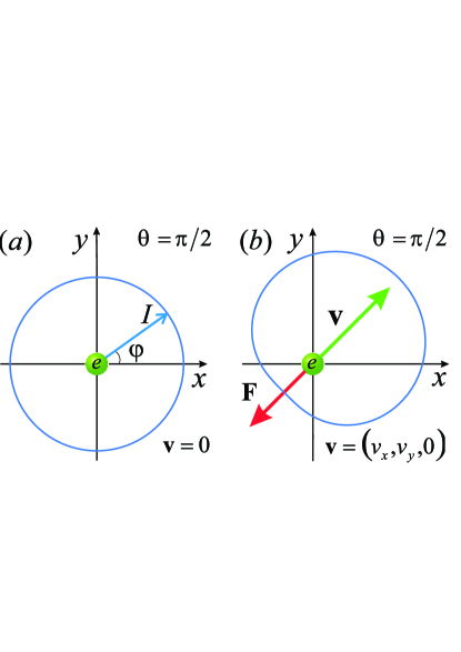
This pattern is of symmetric shape for an electron at rest (see Fig. 1a) but it acquires asymmetry if the electron moves: The intensity of photon emission in the direction of electron velocity $\mathbf{v}$ exceeds the intensity of photon emission in the opposite direction (see Fig. 1b). Due to such a skew photon emission, the resultant momentum transferred to an emitting electron per unit time (the quantum recoil force) differs from zero and reads

$$\mathbf{F}=-\sum_{\mathbf{q}}\hbar\mathbf{q}w({\mathbf{q}})=-\frac{1}{c}\int_{0}^{2\pi}d\varphi\int_{0}^{\pi}d\theta\,\mathbf{n}I(\theta,\varphi),$$ (23)

where $\mathbf{n}=\mathbf{r}/r=(\sin\theta\cos\varphi,\,\sin\theta\sin\varphi,\,\cos\theta)$ is the unit radius vector. Substituting Eq.Β (22) into Eq.Β (23), the recoil force acting on an electron under the field (1) takes the simple final form

$$\mathbf{F}=-\frac{2}{3}\left(\frac{e^{4}\omega^{2}A^{2}_{0}}{m^{2}_{e}c^{7}}\right)\mathbf{v},$$ (24)

where $\mathbf{v}=(v_{x},v_{y},v_{z})$ is the velocity of forward movement of the electron. Applying the classical dynamics equation, $m_{e}\dot{\mathbf{v}}=\mathbf{F}$, to describe evolution of the electron velocity $\mathbf{v}(t)$ under the forceΒ (24), we arrive at the exponentially fast deceleration of the electron,

$$\mathbf{v}(t)=\mathbf{v}(0)e^{-t/\tau_{0}},$$ (25)

where

$$\tau_{0}=\left(\frac{2e^{4}\omega^{2}A^{2}_{0}}{3m^{3}_{e}c^{7}}\right)^{-1}$$ (26)

is the deceleration time. It should be stressed that the forceΒ (24) differs substantially from the Abraham-Lorentz force (also known as Lorentz-Abraham-Dirac force)Β Barut ,

$$\mathbf{F}_{\mathrm{rad}}=\left(\frac{2e^{2}}{3c^{3}}\right)\left[\gamma^{2}\ddot{\mathbf{V}}+\frac{\gamma^{4}\mathbf{V}(\mathbf{V}\cdot\ddot{\mathbf{V}})}{c^{2}}+\frac{3\gamma^{4}\dot{\mathbf{V}}(\mathbf{V}\cdot\dot{\mathbf{V}})}{c^{2}}+{\it{O}}\left(\frac{1}{c^{4}}\right)\right],$$ (27)

introduced into physics in the deep past to describe the radiation reaction within the classical electrodynamics, where ${\mathbf{V}}$ is the velocity of an emitting particle with the charge $e$, and $\gamma=1/\sqrt{1+{V}^{2}/c^{2}}$ is the Lorentz factor. Indeed, substituting the classical velocityΒ (4) into Eq.Β (27) and averaging it over the field period, $2\pi/\omega$, one can see that the averaged force $\mathbf{F}_{\mathrm{rad}}$ turns into zero in contrast to the recoil force (24). Although the forceΒ (24) does not depend explicitly on the Planck constant, $\hbar$, it is purely quantum since its applicability condition (18)–(19) cannot be satisfied in the classical limit of $\hbar\rightarrow 0$. Therefore, there is no classical analogue of the quantum deceleration (25). It should be noted that the deceleration (25) takes place for any charged particles under an oscillating field but it expected to be most pronounced for electrons due to their small mass.

To extend the developed theory for an electron under an electromagnetic wave, the vector potential of the homogeneous field (1) should be replaced by the wave vector potential,

$$\widetilde{\mathbf{A}}_{\pm}=(A_{x},A_{y},A_{z})=A_{0}\Big{(}\cos(\omega t-\mathbf{q}_{0}\mathbf{r}),\,\pm\sin(\omega t-\mathbf{q}_{0}\mathbf{r}),\,0\Big{)},$$ (28)

where $\mathbf{q}_{0}=(0,\,0,\,\omega/c)$ is the wavevector of the wave, the field amplitude is $A_{0}=cE_{0}/\omega$, and $E_{0}$ is the electric field of the wave. The eigenfunctions of the Hamiltonian (2) with the vector potential (28) read

$$\widetilde{\psi}_{\mathbf{k}}=\frac{1}{\sqrt{\cal{V}}}e^{i\mathbf{k}\mathbf{r}}e^{i(\varepsilon_{\mathbf{k}}+\varepsilon_{0})t/\hbar}e^{ik_{x}(1+v_{z}/c)(v_{0}/\omega)\sin\omega t}e^{\mp ik_{y}(1+v_{z}/c)(v_{0}/\omega)\cos\omega t}+{\it{O}}\left(\frac{1}{c^{2}}\right)$$ (29)

and can be easily proved by direct substitution into the SchrΓΆdinger equation, $\hat{\cal H}_{0}\widetilde{\psi}_{\mathbf{k}}=i\hbar\partial_{t}\widetilde{\psi}_{\mathbf{k}}$. Using the Floquet functions (29) as a basis of the expansion (5), we arrive at the probability of photon emission per unit time,

$$\widetilde{w}(\mathbf{q})=\frac{(2\pi)^{5}e^{2}}{cq{\cal{V}}^{2}}\sum_{m=1}^{\infty}\sum_{\mathbf{k}^{\prime}}\left\{\left|\mathbf{\mathbf{e}^{(\mathbf{q})}}\cdot\widetilde{\mathbf{j}}_{\mathbf{k}^{\prime}\mathbf{k}}^{(m)}\right|^{2}\right\}\delta^{3}(\mathbf{k}-\mathbf{k}^{\prime}+m\mathbf{q}_{0}-\mathbf{q})\delta(\varepsilon_{\mathbf{k}}-\varepsilon_{\mathbf{k}^{\prime}}+m\hbar\omega-\hbar cq),$$ (30)

where $\widetilde{\mathbf{j}}_{\mathbf{k}^{\prime}\mathbf{k}}^{(m)}$ are the Fourier harmonics of the transition current in the wave field,

$$\widetilde{\mathbf{j}}_{\mathbf{k}^{\prime}\mathbf{k}}=\frac{1}{2m}\left(\widetilde{\psi}^{\ast}_{\mathbf{k}^{\prime}}\hat{\mathbf{p}}\widetilde{\psi}_{\mathbf{k}}-\widetilde{\psi}_{\mathbf{k}}\hat{\mathbf{p}}\widetilde{\psi}^{\ast}_{\mathbf{k}^{\prime}}\right)-\frac{e}{mc}\widetilde{\mathbf{A}}_{\pm}\widetilde{\psi}^{\ast}_{\mathbf{k}^{\prime}}\widetilde{\psi}_{\mathbf{k}}=\frac{e^{i(\mathbf{k}-\mathbf{k}^{\prime}+m\mathbf{q}_{0})\mathbf{r}}}{\cal{V}}\sum_{m=-\infty}^{\infty}\widetilde{\mathbf{j}}_{\mathbf{k}^{\prime}\mathbf{k}}^{(m)}e^{-im\omega t}.$$ (31)

For the main radiation harmonic ($m=1$), the delta functions in Eq.Β (30) describe the momentum and energy conservation laws,

$$\mathbf{k}+\mathbf{q}_{0}=\mathbf{k}^{\prime}+\mathbf{q},\,\,\,\,\,\varepsilon_{\mathbf{k}}+\hbar\omega=\varepsilon_{\mathbf{k}^{\prime}}+\hbar cq,$$ (32)

which yield the allowed lengths of wave vectors of emitted photons,

$$\widetilde{q}=\frac{\omega}{c}\left[1-\frac{v_{z}}{c}+\frac{\left(\mathbf{v}\cdot\mathbf{n}_{{\mathbf{q}}}\right)}{c}+{\it{O}}\left(\frac{1}{c^{2}}\right)\right].$$ (33)

Taking into account Eqs.Β (16) and (33), the probability (30) in the main order of the $(1/c)$-expansion takes its final form

$\displaystyle\widetilde{w}(\mathbf{q})=\frac{\pi^{2}e^{2}v_{0}^{2}}{\hbar\omega c\cal{V}}\left[\left(1+\frac{2v_{z}}{c}\right)\left(1+\cos^{2}\theta_{\mathbf{q}}\right)+\frac{2v_{x}}{c}\cos^{2}\theta_{\mathbf{q}}\sin\theta_{\mathbf{q}}\cos\varphi_{\mathbf{q}}+\frac{2v_{y}}{c}\cos^{2}\theta_{\mathbf{q}}\sin\theta_{\mathbf{q}}\sin\varphi_{\mathbf{q}}-\frac{2v_{z}}{c}\cos\theta_{\mathbf{q}}\sin^{2}{\theta_{\mathbf{q}}}\right.$
$\displaystyle+\left.{\it{O}}\left(\frac{1}{c^{2}}\right)\right]\delta(q-\widetilde{q}).$ (34)

Applying Eq.Β (III) to find the recoil force acting on an electron in the wave field, $\mathbf{F}=-\sum_{\mathbf{q}}\hbar\mathbf{q}\widetilde{w}({\mathbf{q}})$, one can see that it is described by the same expression (24). It follows from the conservation laws (32) that the considered emission process in the wave field (28) is physically identical to the Compton scattering of the wave by the electron. Particularly, emission (scattering) of each photon is accompanied by transfer of the momentum $\hbar\mathbf{q}_{0}$ from the wave to the electron. As a consequence, the photon drag force,

$$\mathbf{F}_{0}=\hbar\mathbf{q}_{0}\sum_{\mathbf{q}}\widetilde{w}(\mathbf{q})=\hbar\mathbf{q}_{0}\sum_{\mathbf{q}}{w}(\mathbf{q})=\frac{2}{3}\left(\frac{e^{4}\omega^{2}A^{2}_{0}}{m^{2}_{e}c^{6}}\right)\mathbf{n}_{0},$$ (35)

occurs in addition to the recoil force (24), where $\mathbf{n}_{0}=\mathbf{q}_{0}/q_{0}$ is the unit wavevector. As expected, the photon drag force (35) exactly coincides with the known radiation pressure force acting on an electron under an electromagnetic wave, which was derived earlier from the scattering theoryΒ Bohm .

The electron dynamics under the two forces (24) and (35) can be described by the classical equation, $m_{e}\dot{\mathbf{v}}=\mathbf{F}_{0}+\mathbf{F}$. For a non-relativistic electron, $v\ll c$, the force (35) much exceeds the force (24). Therefore, the photon drag force $\mathbf{F}_{0}$ accelerates an electron along the direction of wave propagation, whereas the recoil force $\mathbf{F}$ decelerates it in the perpendicular directions. As a result, the alignment of electron velocities occurs: During the time $t\gg\tau_{0}$, velocities of free electrons exposed to an electromagnetic wave become oriented along the direction of wave propagation. This can lead, particularly, to collecting and focusing of an electron beam under laser irradiation. In two-dimensional electron systems (e.g., conduction electrons in quantum wells and other two-dimensional nanostructures) irradiated by a normally incident electromagnetic wave, the photon drag force (35) vanishes, whereas the recoil force (24) results in the cooling of electrons. If the two-dimensional electron gas is non-degenerate, the averaged electron velocity is $\langle v\rangle=\sqrt{8k_{B}T/\pi m_{e}}$, where $T$ is the temperature of the gas, and $k_{B}$ is the Boltzmann constant. Then the deceleration (25) leads to exponentially fast decreasing electron temperature, $T(t)=T(0)e^{-2t/\tau_{0}}$. It should be noted that the theory developed above for the circularly polarized fields (1) and (28) can be easily generalized for any field polarization. For a linearly polarized field, particularly, the recoil and photon drag forces are described by the same expressions (24) and (35), where the numerical factor $2/3$ in the right-hand side should only be replaced by the factors $1/15$ and $1/3$, respectively.

It follows from the aforesaid that the deceleration time (26) should be small enough to observe the discussed effects experimentally, which needs intense laser fields. For an electromagnetic wave generated by an ordinary hundred-kilowatt laser with the wavelengths $\lambda\sim 10^{-6}$Β m, the electric field amplitude $E_{0}$ can reach $10^{10}$Β V/m, which corresponds to the deceleration time (26) of a split second. One can expect that this time scale is appropriate to detect the electron deceleration in state-of-the-art measurements. The discussed effects can manifest themselves in various electronic systems, including free electrons in vacuum and conduction electrons in condensed matters. Among them, semiconductor structures hold much promise since the effective electron mass can be very small there. Electrons in graphene and related materials also deserve careful consideration since their kinetic energy can be very large under low-power irradiation due to the giant Fermi velocityΒ Kibis_2010 . It should be stressed that controlling electronic properties of various condensed-matter structures by a high-frequency off-resonant electromagnetic field β€” which is based on the Floquet theory of periodically driven quantum systems (β€œFloquet engineering”) β€” has become an established research area during last decades and lead to many light-induced quantum phenomena (see, e.g., Refs.Β Kibis_2010, ; Basov_2017, ; Oka_2019, ; Kobayashi_2023, ; Kibis_2011, ; Nuske_2020, ; Lindner_2011, ; Rechtsman_2013, ; Wang_2013, ; Sie_2015, ; Cavalleri_2020, and references therein). Therefore, the discussed high-frequency mechanism of electron deceleration can be considered, particularly, as a tool to manipulate conduction electrons in condensed matters, which fits well the current trend in modern physics.

IV Conclusion

It is shown theoretically that an electron oscillating under a high-frequency electromagnetic field emits photons differently in the direction of its forward movement and in the opposite direction. Since emission of each photon is accompanied by momentum transfer to the electron, such a skew emission leads to the quantum recoil force decelerating the forward movement of the electron. This quantum phenomenon is of general physical nature and can manifest itself in various electronic systems driven by a laser field, including free electrons in vacuum and conduction electrons in condensed matters. It can lead, particularly, to the alignment of velocities of free electrons along the direction of laser beam and the laser-induced cooling of conduction electrons confined in two-dimensional nanostructures.

References

  • (1) L. D. Landau and E. M. Lifshitz, The Classical Theory of Fields (Pergamon Press, Oxford, 1987).
  • (2) N. Goldman and J. Dalibard, Periodically driven quantum systems: Effective Hamiltonians and engineered gauge fields, Phys. Rev. X 4, 031027 (2014).
  • (3) M. Bukov, L. D’Alessio, and A. Polkovnikov, Universal high-frequency behavior of periodically driven systems: From dynamical stabilization to Floquet engineering, Adv. Phys. 64, 139 (2015).
  • (4) A. Eckardt and E. Anisimovas, High-frequency approximation for periodically driven quantum systems from a Floquet-space perspective, New J. Phys. 17, 093039 (2015).
  • (5) F. Casas, J. A. Oteo, and J. Ros, Floquet theory: Exponential perturbative treatment, J. Phys. A 34, 3379 (2001).
  • (6) O. V. Kibis, Floquet theory of spin dynamics under circularly polarized light pulses, Phys. Rev. A 105, 043106 (2022).
  • (7) L. D. Landau and E. M. Lifshitz, Quantum Mechanics: Nonrelativistic Theory (Pergamon Press, Oxford, 1991).
  • (8) V. B. Berestetskii, E. M. Lifshitz, and L. P. Pitaevskii, Quantum Electrodynamics (Pergamon Press, Oxford, 1982).
  • (9) A. O. Barut, Electrodynamics and Classical Theory of Fields & Particles (Dover Publications, New York, 1980), p.Β 184–185.
  • (10) D. Bohm, Quantum Theory (Prentice Hall, New York, 1951), p.Β 34.
  • (11) O. V. Kibis, Metal-insulator transition in graphene induced by circularly polarized photons, Phys. Rev. B 81, 165433 (2010).
  • (12) D. N. Basov, R. D. Averitt, and D. Hsieh, Towards properties on demand in quantum materials, Nat. Mater. 16, 1077 (2017).
  • (13) T. Oka and S. Kitamura, Floquet Engineering of Quantum Materials, Annu. Rev. Condens. Matter. Phys. 10, 387 (2019).
  • (14) Y. Kobayashi, C. Heide, A. C. Johnson, V. Tiwari, F. Liu, D. A. Reis, T. F. Heinz and S. Ghimire, Floquet engineering of strongly driven excitons in monolayer tungsten disulfide, Nat. Phys. 19, 171 (2023).
  • (15) O. V. Kibis, Dissipationless electron transport in photon-dressed nanostructures, Phys. Rev. Lett. 107, 106802 (2011).
  • (16) M. Nuske, L. Broers, B. Schulte, G. Jotzu, S. A. Sato, A. Cavalleri, A. Rubio, J. W. McIver, and L. Mathey, Floquet dynamics in light-driven solids, Phys. Rev. Res. 2, 043408 (2020).
  • (17) N. H. Lindner, G. Refael, and V. Galitski, Floquet topological insulator in semiconductor quantum wells, Nat. Phys. 7, 490 (2011).
  • (18) M. C. Rechtsman, J. M. Zeuner, Y. Plotnik, Y. Lumer, D. Podolsky, F. Dreisow, S. Nolte, M. Segev, and A. Szameit, Photonic Floquet topological insulator, Nature 496, 196 (2013).
  • (19) Y. H. Wang, H. Steinberg, P. Jarillo-Herrero, and N. Gedik, Observation of Floquet-Bloch states on the surface of a topological insulator, Science 342, 453 (2013).
  • (20) E. J. Sie, J. W. McIver, Y.-H. Lee, L. Fu, J. Kong, and N. Gedik, Valley-selective optical Stark effect in monolayer WS2, Nat. Mater. 14, 290 (2015).
  • (21) J. W. McIver, B. Schulte, F.-U. Stein, T. Matsuyama, G. Jotzu, G. Meier, and A. Cavalleri, Light-induced anomalous Hall effect in graphene, Nat. Phys. 16, 38 (2020).