On linear quadratic regulator for the heat equation with general boundary conditions

Abstract

We consider the linear quadratic regulator of the heat equation on a finite interval. Previous frequency-domain methods for this problem rely on discrete Fourier transform and require symmetric boundary conditions. We use the Fokas method to derive the optimal control law for general Dirichlet and Neumann boundary conditions. The Fokas method uses the continuous Fourier transform restricted to the bounded spatial domain, with the frequency domain extended from the real line to the complex plane. This extension, together with results from complex analysis, allows us to eliminate the dependence of the optimal control on the unknown boundary values. As a result, we derive an integral representation of the control similar to the inverse Fourier transform. This representation contains integrals along complex contours and only depends on known initial and boundary conditions. We also show that for the homogeneous Dirichlet boundary value problem, the integral representation recovers an existing series representation of the optimal control. Moreover, the integral representation exhibits numerical advantages compared to the traditional series representation.

I Introduction

Following the seminal paper [1], there has been a great interest in optimal control of spatially invariant systems using frequency-domain methods, e.g., see [2, 3]. Spatially invariant systems are defined without boundaries, while most real-world systems are defined on finite spatial domains with boundary conditions. Although spatially invariant systems can be seen as approximations of large-scale but finite-extent systems, e.g., in [4], the effect of boundary conditions is not considered in this approximation.

Only a few studies target finite-extent systems with boundary conditions; see [5, 6]. Both studies assumed symmetric boundary conditions and approached the problem by embedding finite-extent systems into equivalent spatially invariant systems. The embedding technique is motivated by the method of images that is used to solve boundary value problems for linear partial differential equations (PDEs) with some symmetry properties. Hence, their methods are also limited to certain symmetric boundary conditions. Although the control of finite systems with general boundary conditions is still quite open, studies have discussed potential extensions to estimation problem [7].

Recently, a unified approach, also known as the Fokas method, has been developed to provide solutions to linear and a class of nonlinear PDEs with general boundary conditions, see [8, 9, 10, 11]. Traditionally, linear PDEs with different types of boundary conditions require different specialized methods to obtain solutions. For example, sine transform and series are used for Dirichlet boundary value problems, and cosine transform and series are used for Neumann boundary value problems. In contrast to these specific approaches, the Fokas method uses only the Fourier transform to obtain solutions for all types of boundary conditions, with the frequency variable $k$ extended to the complex domain. Since the Fourier transform was initially used to analyze the optimal control of spatially invariant systems in [1], it is natural to explore the control of finite-extent systems with boundary conditions using the Fokas method.

Unlike the boundary control setting previously dealt with by the Fokas method in [12], the linear quadratic control appears in PDEs as a forcing term that depends on the states and boundary conditions. Still, we show that the Fokas method can derive an integral representation of the optimal control. Furthermore, the integral control law results in an integral representation of the state that uniformly converges to the boundary conditions, while the series representation does not for nonzero boundary conditions. Also, the numerical computation of integral representations is much easier than computing series representations. It is important to note that the Fokas method applies to general linear PDEs. Thus, our approach can be extended to other linear PDEs, beyond the heat equation.

The contributions of the paper are as follows. First, we derive the control law in the complex domain for the linear quadratic regulator of the heat equation using the unified Fourier transform. The optimal control law depends on the Neumann and Dirichlet boundary conditions, whereas only one of these two is given. Second, we derive an integral representation of the optimal control that depends only on the given initial and boundary conditions and thus can be directly evaluated. Third, we show that the integral representation is equivalent to the series representation of the optimal control in [6] for the homogeneous Dirichlet boundary value problem. We numerically evaluate our integral representation of the control and demonstrate its numerical advantages over the series representation.

The paper is organized as follows: we formulate the linear quadratic regulator problem for the heat equation in Section II. Then, we derive the transformed optimal control law in Section III. We consider the special case of infinite-time control in Section IV. Section V derives the integral representation of the optimal control. We compare our integral representation of the control and an existing control form in Section VI. Section VII concludes our findings and gives future directions.

II Problem formulation

Consider the following heat equation in the domain $\Omega=\{0<x<L,t>0\}$, with distributed heat injection $u(x,t)$

$$\phi_{t}=\phi_{xx}+u(x,t),$$ (1)

and initial condition $\phi(x,0)=\phi_{0}(x),0<x<L$. We will denote the Dirichlet and Neumann boundary values by $g_{0},h_{0}$ and $g_{1},h_{1}$, i.e.,

$$\phi(0,t)=g_{0}(t),\ \phi(L,t)=h_{0}(t), t>0;$$ (2)

$$\phi_{x}(0,t)=g_{1}(t),\ \phi_{x}(L,t)=h_{1}(t), t>0.$$

Either the pair of Dirichlet boundary values $g_{0},h_{0}$ or Neumann boundary values $g_{1},h_{1}$ is provided. Our goal is to find an optimal control $u^{*}(x,t),x\in(0,L),t\in(0,T]$, minimizing the objective functional

$$J=\int_{0}^{T}\int_{0}^{L}\left[\phi^{2}(x,t)+u^{2}(x,t)\right]\mathop{}\!\mathrm{d}x\ \mathop{}\!\mathrm{d}t+\int_{0}^{L}\phi^{2}(x,T)\mathop{}\!\mathrm{d}x$$ (3)

subject to dynamics (1). The main challenge is the unknown relation between the known and unknown boundary values. We will use the Fokas method to represent the unknown boundary values in terms of given initial boundary conditions.

III The transformed finite-time optimal control law

First, we show how to derive the optimal control law in the complex domain using the unified transform [10]. The unified transform is the Fourier transform restricted in the domain $0<x<L$ with $k$ extended to the complex domain $\mathbb{C}$:

$$\hat{f}(k) =\int_{0}^{L}e^{-ikx}f(x)\mathop{}\!\mathrm{d}x,\quad k\in\mathbb{C},\,$$ (4)

$$f(x) =\int_{-\infty}^{\infty}\hat{f}(k)e^{ikx}\frac{\mathop{}\!\mathrm{d}k}{2\pi},\quad 0<x<L.$$ (5)

Remark 1

The unified transform can be regarded as the direct and inverse Fourier transform applied to the following function

$$F(x)=\left\{\begin{aligned} &f(x),&0<x<L,\\ &0,&\text{otherwise}.\end{aligned}\right.$$

Let $\hat{\phi}$ and $\hat{u}$ denote the unified transform of $\phi$ and $u$ by (4). We start by taking a derivative with respect to $t$ and then use the relation (1):

$$\frac{\partial\hat{\phi}}{\partial t} =\int_{0}^{L}e^{-ikx}\phi_{t}(x,t)\mathop{}\!\mathrm{d}x$$

$$=\int_{0}^{L}e^{-ikx}\phi_{xx}(x,t)\mathop{}\!\mathrm{d}x+\hat{u}(k,t).$$

Using integration by parts, we have

$$\int_{0}^{L}e^{-ikx}\phi_{xx}\mathop{}\!\mathrm{d}x$$

$$=e^{-ikL}\phi_{x}(L,t)-\phi_{x}(0,t)+ik\int_{0}^{L}e^{-ikx}\phi_{x}(x,t)\mathop{}\!\mathrm{d}x.$$

$$=e^{-ikL}\phi_{x}(L,t)-\phi_{x}(0,t)$$

$$+ik\left[e^{-ikL}\phi(L,t)-\phi(0,t)+ik\int_{0}^{L}e^{-ikL}\phi(x,t)\mathop{}\!\mathrm{d}x\right]$$

Introducing the notation specified earlier, we find

$$\dfrac{\partial\hat{\phi}}{\partial t}=-k^{2}\hat{\phi}+\hat{u}(k,t)+v_{1}(k,t),$$ (6)

where

$$v_{1}(k,t):=-g_{1}(t)-ikg_{0}(t)+e^{-ikL}\left(h_{1}(t)+ikh_{0}(t)\right).$$ (7)

(6) is an ordinary differential equation (ODE) in the time variable.

Remark 2

The inverse transform (5) involves real $k$, and thus we only need $\hat{\phi}(k,t)$ for real $k$ in (6). However, we will find it useful to detour from the real line to the complex plane.

Parseval’s identity implies that minimizing (3) is the same as finding $\hat{u}$ that minimizes

$$\hat{J}=\int_{-\infty}^{\infty}\left[\int_{0}^{T}\left(\hat{\phi}^{2}(k,t)+\hat{u}^{2}(k,t)\right)dt+\hat{\phi}^{2}(k,T)\right]\mathop{}\!\mathrm{d}k$$ (8)

subject to (6) and $\hat{\phi}(k,0)=\hat{\phi}_{0}(k).$ Since (6) is an ODE in the time variable parameterized by $k$, at a fixed $k$ it amounts to no more than a classical finite-dimensional linear quadratic regulator problem.

Theorem 1

The optimal control for (8) subject to (6) is given by

$$\hat{u}^{*}(k,t)=-\hat{p}(k,t)\hat{\phi}(k,t)-\dfrac{1}{2}v_{1}(k,t)r_{1}(k,t)-\frac{1}{2}r_{2}(k,t),$$ (9)

where for all $k$, $\hat{p}(k,t)$ and $\mathbf{r}(k,t):=\begin{bmatrix}r_{1}(k,t)&r_{2}(k,t)\end{bmatrix}$ are solutions to the following equations

$$-\hat{p}_{t} =1-2k^{2}\hat{p}-\hat{p}^{2},\quad\hat{p}(k,T)=1,$$ (10)

$$-\mathbf{Q}_{t} =2\mathbf{Q}\,\mathbf{M}(k,t)+\mathbf{r}\,\mathbf{d}^{\top}-\dfrac{1}{4}\mathbf{r}\,\mathbf{r}^{\top},\quad\mathbf{Q}(k,T)=\mathbf{0}_{2\times 2},$$ (11)

$$-\mathbf{r}_{t} =-k^{2}\,\mathbf{r}+\mathbf{M}(k,t)^{\top}\mathbf{r}-\hat{p}\,\mathbf{r}+2\hat{p}\,\mathbf{d},\quad\mathbf{r}(k,T)=\mathbf{0}_{2\times 1}$$ (12)

with $\mathbf{d}=\begin{bmatrix}1\\ 0\end{bmatrix},\mathbf{M}(k,t)=\begin{bmatrix}0&\frac{\partial v_{1}}{\partial t}\\ 0&0\end{bmatrix}.$

Proof:

It is convenient to rewrite (9) as

$$\hat{u}^{*}(k,t)=-\hat{p}(k,t)\hat{\phi}(k,t)-\dfrac{1}{2}\mathbf{v}(k,t)^{\top}\mathbf{r}(k,t),$$

where $\mathbf{v}(k,t)=\begin{bmatrix}v_{1}(k,t)&1\end{bmatrix}^{\top}$. For any fixed $k$, we omit the dependence on $k$ in variables $\hat{\phi}$ and $\hat{u}$ and rewrite (6) as a linear time-varying system:

$$\hat{\phi}_{t} =-k^{2}\hat{\phi}+\hat{u}+\mathbf{d}^{\top}\mathbf{v},$$ (13)

$$\mathbf{v}_{t} =\mathbf{M}(t)\,\mathbf{v}$$

with $\mathbf{d},\mathbf{M}$ defined in Theorem 1. The control problem is now to find an $\hat{u}^{*}(t),t\in[0,T]$, minimizing

$$V(\hat{\phi}(0),\mathbf{v}(0),\hat{u}(\cdot),0)=\int_{0}^{T}\left[\hat{\phi}^{2}(\tau)+\hat{u}^{2}(\tau)\right]\mathop{}\!\mathrm{d}\tau+\hat{\phi}^{2}(T)$$

subject to (13).

We use the principle of optimality, also known as dynamic programming, to derive the optimal control. Let $\hat{u}[a,b]$ denote a function $u(\cdot)$ restricted to the interval $[a,b]$. Given $t\in[0,T]$, let us also make the definition

$$V^{*}(\hat{\phi},\mathbf{v},t):=\min_{\hat{u}[t,T]}\ V(\hat{\phi},\mathbf{v},\hat{u},t).$$ (14)

Two properties of the optimal value function (14) [13, Eq.2.2-5, Eq.2.3-7] applied to dynamics (13) are stated as follows.

Lemma 1

The optimal value function $V^{*}(\hat{\phi},\mathbf{v},t)$ satisfies the Hamilton-Jacobi-Bellman equation:

$$\pdv{}{t}V^{*}(\hat{\phi},\mathbf{v},t)\\ =-\min_{\hat{u}(t)}\Big{\{}\hat{\phi}^{2}(t)+\hat{u}^{2}(t)+\pdv{}{\hat{\phi}}V^{*}(\hat{\phi},\mathbf{v},t)\hat{\phi}_{t}\\ +\left[\pdv{}{\mathbf{v}}V^{*}(\hat{\phi},\mathbf{v},t)\right]^{\top}\mathbf{v}_{t}\Big{\}}$$ (15)

with the boundary condition $V^{*}(\hat{\phi}(T),\mathbf{v}(T),T)=\hat{\phi}^{2}(T)$, and the control given by the minimization in (15) is the optimal control $\hat{u}^{*}(t)$ at time $t$.

Lemma 2

The optimal value function $V^{*}(\hat{\phi},\mathbf{v},t)$ has the quadratic form

$$V^{*}(\hat{\phi},\mathbf{v},t)=\hat{p}(t)\hat{\phi}^{2}+\mathbf{v}^{\top}\mathbf{Q}(t)\mathbf{v}+\mathbf{v}^{\top}\mathbf{r}(t)\hat{\phi},$$

where $\mathbf{Q}(t)$ is symmetric.

Using Lemma 2, we can solve $\eqref{eq:hjb}$ to obtain the optimal control. From Lemma 2, the left-hand side in (15) becomes

$$\pdv{V^{*}}{t}(\hat{\phi},\mathbf{v},t)=\hat{p}_{t}\hat{\phi}^{2}+\mathbf{v}^{\top}\mathbf{Q}_{t}\mathbf{v}+\mathbf{v}^{\top}\mathbf{r}_{t}\,\hat{\phi}.$$ (16)

The terms with partial derivatives on the right-hand side become

$$\pdv{V^{*}}{\hat{\phi}}(\hat{\phi},\mathbf{v},t)\hat{\phi}_{t}=(2\hat{p}(t)\hat{\phi}+\mathbf{v}^{\top}\mathbf{r}(t))(-k^{2}\hat{\phi}+\hat{u}+\mathbf{d}^{\top}\mathbf{v}),$$

$$\left[\pdv{V^{*}}{\mathbf{v}}(\hat{\phi},\mathbf{v},t)\right]^{\top}\mathbf{v}_{t}=(2\mathbf{v}^{\top}\mathbf{Q}(t)+\hat{\phi}\,\mathbf{r}(t)^{\top})\mathbf{M}(t)\mathbf{v}.$$

Substitute the above terms into the right-hand side in (15) and complete the square, we have

$$\hat{\phi}^{2}+\hat{u}^{2}+\pdv{V^{*}}{\hat{\phi}}(\hat{\phi},\mathbf{v},t)\hat{\phi}_{t}+\left[\pdv{V^{*}}{\mathbf{v}}(\hat{\phi},\mathbf{v},t)\right]^{\top}\mathbf{v}_{t}$$ (17)

$$= (\hat{u}+\hat{p}(t)\hat{\phi}+\dfrac{1}{2}\mathbf{v}^{\top}\mathbf{r}(t))^{2}$$

$$+(1-2k^{2}\hat{p}(t)-\hat{p}^{2}(t))\hat{\phi}^{2}$$

$$+\mathbf{v}^{\top}(2\mathbf{Q}(t)\mathbf{M}(t)+\mathbf{r}(t)\mathbf{d}^{\top}-\dfrac{1}{4}\mathbf{r}(t)\mathbf{r}(t)^{\top})\mathbf{v}$$

$$+\mathbf{v}^{\top}(-k^{2}\mathbf{r}(t)+\mathbf{M}(t)^{\top}\mathbf{r}(t)-\hat{p}(t)\mathbf{r}(t)+2\hat{p}(t)\mathbf{d})\hat{\phi}.$$

Therefore, the minimization in (15) is achieved by

$$\hat{u}^{*}(t)=-\hat{p}(t)\hat{\phi}(t)-\dfrac{1}{2}\mathbf{v}(t)^{\top}\mathbf{r}(t).$$ (18)

Substitute (18) into (17) and equate (16), together with the boundary condition $V^{*}(\hat{\phi}(T),\mathbf{v}(T),T)=\hat{\phi}^{2}(T)$, we have

$$-\hat{p}_{t} =1-2k^{2}\hat{p}-\hat{p}^{2},\quad\hat{p}(T)=1$$

$$-\mathbf{Q}_{t} =2\mathbf{Q}\,\mathbf{M}(t)+\mathbf{r}\,\mathbf{d}^{\top}-\dfrac{1}{4}\mathbf{r}\,\mathbf{r}^{\top},\mathbf{Q}(T)=\mathbf{0}_{2\times 2}$$

$$-\mathbf{r}_{t} =-k^{2}\,\mathbf{r}+\mathbf{M}(t)^{\top}\mathbf{r}-\hat{p}\,\mathbf{r}+2\hat{p}\,\mathbf{d},\mathbf{r}(T)=\mathbf{0}_{2\times 1}$$

∎

IV The infinite-time optimal control law

In the case of infinite-time control, i.e., $T\to\infty$, (9) still holds, and we disregard the terminal cost $\hat{\phi}^{2}(k,T)$. Then, the initial condition for $\hat{p}$ becomes $\hat{p}(k,T)=0$. For every $k$ in the complex plane and every finite $t$, the solution to (10) starting from $\hat{p}(k,T)=0$ with $T\to\infty$ converges to the equilibrium with nonnegative real value, which is a root to the following:

$$1-2k^{2}\hat{p}(k)-\hat{p}(k)^{2}=0.$$ (19)

For $\mathbf{r}(k,t)$, (12) can be explicitly written as

$$-r_{1t} =-(k^{2}+\hat{p}(k))r_{1}+2\hat{p}(k), r_{1}(T)=0,$$ (20)

$$-r_{2t} =-(k^{2}+\hat{p}(k))r_{2}+r_{1}\frac{\partial v_{1}}{\partial t}, r_{2}(T)=0.$$ (21)

Let $\omega(k):=\sqrt{k^{4}+1}.$ Solving the above equations we find

$$\hat{p}(k) \!=\!-k^{2}+\omega(k),$$

$$r_{1}(k) \!=\!2\hat{p}(k)\int^{\infty}_{t}e^{\omega(k)(t-\xi)}\mathop{}\!\mathrm{d}\xi=\dfrac{2\hat{p}(k)}{\omega(k)},$$

$$r_{2}(k,t) \!=\!r_{1}(k)\int^{\infty}_{t}e^{\omega(k)(t-\xi)}\frac{\partial v_{1}}{\partial\xi}\mathop{}\!\mathrm{d}\xi$$

$$\!=\!r_{1}(k)(-v_{1}(k,t)\!+\!\omega(k)\int_{t}^{\infty}e^{\omega(k)(t-\xi)}v_{1}(k,\xi)\!\mathop{}\!\mathrm{d}\xi).$$

Using the above expressions in (9), we find an infinite-time optimal control law in the complex domain:

$$\hat{u}^{*}(k,t)=-\hat{p}(k)\hat{\phi}(k,t)-\hat{p}(k)\int_{t}^{\infty}e^{\omega(k)(t-\xi)}v_{1}(k,\xi)\mathop{}\!\mathrm{d}\xi.$$ (22)

Substitute (22) into (6), we have

$$\dfrac{\partial\hat{\phi}}{\partial t}=-\omega(k)\hat{\phi}+v_{1}(k,t)-\hat{p}(k)\int_{t}^{\infty}e^{\omega(k)(t-\xi)}v_{1}(k,\xi)\mathop{}\!\mathrm{d}\xi.$$ (23)

Now, we analyze the well-posedness and stability of the heat equation (1) after substituting optimal control (22). Unlike traditional methods that represent PDEs in abstract differential equations, e.g., see [14], the Fourier transform decomposes the heat equation into an ODE (23) for each $k$. Therefore, it suffices to analyze the well-posedness and stability of the ODE for each $k$. Let $b(k,t):=v_{1}(k,t)-\hat{p}(k)\int_{t}^{\infty}e^{\omega(k)(t-\xi)}v_{1}(k,\xi)\mathop{}\!\mathrm{d}\xi$. The solution to (23) with the transformed initial condition $\hat{\phi}(k,0)=\hat{\phi}_{0}(k)$ is given by

$$\hat{\phi}(k,t)=e^{-\omega(k)t}\hat{\phi}_{0}(k)+\int_{0}^{t}e^{-\omega(k)(t-\xi)}b(k,\xi)\mathop{}\!\mathrm{d}\xi.$$

For simplicity, we assume that $v_{1}(\cdot,\cdot)$ is bounded, and there exists a finite time $K$ such that $v_{1}(k,t)=0$ for all $t>K$. Then, $b(k,t)=0$ for all $t>K$. Following Remark 2, for every real $k$, the solution $\hat{\phi}(k,t)$ is unique, and $\hat{\phi}(k,t)\to 0$ as $t\to\infty$ since $\omega(k)>0$. Tighter conditions for well-posedness and stability can be obtained through more complicated analysis and will be pursued in the future.

V The integral representation of the optimal control

After obtaining the control law (22) in the transformed domain, we aim to derive an expression of the optimal control $u^{*}(x,t)$ in the original space domain. Combining (22) and (23), we have

$$\hat{u}^{*}(k,t)=\dfrac{\partial\hat{\phi}}{\partial t}+k^{2}\hat{\phi}-v_{1}(k,t).$$ (24)

Applying the inverse transform (5) to (24), we have

$$u^{*}(x,t)=\phi_{t}(x,t)+\int_{-\infty}^{\infty}e^{ikx}\left[k^{2}\hat{\phi}(k,t)-v_{1}(k,t)\right]\frac{\mathop{}\!\mathrm{d}k}{2\pi}.$$ (25)

The control law (25) cannot be computed yet since only one of the Dirichlet and Neumann boundary conditions in $v_{1}(k,t)$ is provided, i.e., either $(g_{0}(t),h_{0}(t))$ or $(g_{1}(t),h_{1}(t))$ is known. We will derive an expression of $u^{*}(x,t)$ that depends only on given initial and boundary conditions. In the following result, we consider the case that Dirichlet boundary conditions are given:

Theorem 2

Given Dirichlet boundary values $g_{0}(t),h_{0}(t)$ for all $t>0,$ the optimal control $u^{*}(x,t)$ in the domain $\Omega$ is given by

$$u^{*}(x,t)=-\int_{-\infty}^{\infty}e^{ikx-\omega(k)t}\,\hat{p}(k)\hat{\phi}_{0}(k)\dfrac{\mathop{}\!\mathrm{d}k}{2\pi}$$ (26)

$$+\int_{\partial\mathcal{D}^{+}}\dfrac{e^{-\omega(k)t}\hat{p}(k)}{e^{ikL}-e^{-ikL}}\Big{\{}2\sin(kx)\big{[}ie^{ikL}\hat{\phi}_{0}(k)$$

$$\hskip 36.135pt-2k(\tilde{h}_{0}(\omega(k),t))-\hat{p}(k)\bar{h}_{0}(\omega(k),t))\big{]}$$

$$\hskip 36.135pt+2\sin(k(L-x))\big{[}i\hat{\phi}_{0}(-k)$$

$$\hskip 36.135pt-2k(\tilde{g}_{0}(\omega(k),t)-\hat{p}(k)\bar{g}_{0}(\omega(k),t)\big{]}\Big{\}}\dfrac{\mathop{}\!\mathrm{d}k}{2\pi}$$

$$-\int_{\partial\mathcal{D}^{+}}\dfrac{1}{e^{ikL}-e^{-ikL}}\Big{\{}2\sin(kx)$$

$$\hskip 36.135pt\big{[}-2kh_{0}(t)-\hat{p}(k)\underline{h}_{0}(\omega(k),t)\big{]}+2\sin(k(L-x))$$

$$\hskip 36.135pt\big{[}-2kg_{0}(t)-\hat{p}(k)\underline{g}_{0}(\omega(k),t)\big{]}\Big{\}}\frac{\mathop{}\!\mathrm{d}k}{2\pi},$$

where $\partial\mathcal{D}^{+}$ is a contour in $\mathbb{C}^{+}$ defined as $\partial\mathcal{D}^{+}:=\{k\in\mathbb{C}^{+}:k=\left|k\right|e^{i\theta},\theta=\pi/8\text{ or }7\pi/8\}$;

$$\tilde{g}_{0}(k,t) :=\int_{0}^{t}e^{k\tau}g_{0}(\tau)\mathop{}\!\mathrm{d}\tau,\quad\tilde{h}_{0}(k,t):=\int_{0}^{t}e^{k\tau}h_{0}(\tau)\mathop{}\!\mathrm{d}\tau,$$ (27)

$$\underline{g}_{0}(k,t) :=\int_{\tau}^{\infty}e^{k(\tau-\xi)}g_{0}(\xi)\mathop{}\!\mathrm{d}\xi,$$

$$\underline{h}_{0}(k,t) :=\int_{\tau}^{\infty}e^{k(\tau-\xi)}h_{0}(\xi)\mathop{}\!\mathrm{d}\xi,$$

$$\bar{g}_{0}(k,t) :=\int_{0}^{t}e^{k\tau}\underline{g}_{0}(k,\tau)\mathop{}\!\mathrm{d}\tau,$$

$$\bar{h}_{0}(k,t) :=\int_{0}^{t}e^{k\tau}\underline{h}_{0}(k,\tau)\mathop{}\!\mathrm{d}\tau.$$

Remark 3

The optimal control (26) only depends on given initial and boundary values. Similar expressions can be derived if Neumann boundary values are given.

Proof:

Following (25), the optimal control is computed by taking the time derivative of

$$\phi(x,t)=\int_{-\infty}^{\infty}e^{ikx}\hat{\phi}(k,t)\frac{\mathop{}\!\mathrm{d}k}{2\pi}$$ (28)

$$=\int_{-\infty}^{\infty}e^{ikx-\omega(k)t}\,\hat{\phi}_{0}(k)\dfrac{\mathop{}\!\mathrm{d}k}{2\pi}$$

$$-\int_{\partial\mathcal{D}^{+}}\dfrac{e^{-\omega(k)t}}{e^{ikL}-e^{-ikL}}\Big{\{}2\sin(kx)\big{[}ie^{ikL}\hat{\phi}_{0}(k)$$

$$\hskip 36.135pt-2k(\tilde{h}_{0}(\omega(k),t))-\hat{p}(k)\bar{h}_{0}(\omega(k),t))\big{]}$$

$$\hskip 36.135pt+2\sin(k(L-x))\big{[}i\hat{\phi}_{0}(-k)$$

$$\hskip 36.135pt-2k(\tilde{g}_{0}(\omega(k),t)-\hat{p}(k)\bar{g}_{0}(\omega(k),t)\big{]}\Big{\}}\dfrac{\mathop{}\!\mathrm{d}k}{2\pi}$$

plus

$$\int_{-\infty}^{\infty}e^{ikx}k^{2}\hat{\phi}(k,t)\frac{\mathop{}\!\mathrm{d}k}{2\pi}$$ (29)

$$=\int_{-\infty}^{\infty}e^{ikx-\omega(k)t}\,k^{2}\hat{\phi}_{0}(k)\dfrac{\mathop{}\!\mathrm{d}k}{2\pi}$$

$$-\int_{\partial\mathcal{D}^{+}}\dfrac{e^{-\omega(k)t}k^{2}}{e^{ikL}-e^{-ikL}}\Big{\{}2\sin(kx)\big{[}ie^{ikL}\hat{\phi}_{0}(k)$$

$$\hskip 36.135pt-2k(\tilde{h}_{0}(\omega(k,t))-\hat{p}(k)\bar{h}_{0}(\omega(k),t))\big{]}$$

$$\hskip 36.135pt+2\sin(k(L-x))\big{[}i\hat{\phi}_{0}(-k)$$

$$\hskip 36.135pt-2k(\tilde{g}_{0}(\omega(k),t)-\hat{p}(k)\bar{g}_{0}(\omega(k),t)\big{]}\Big{\}}\dfrac{\mathop{}\!\mathrm{d}k}{2\pi}$$

and the following integral that vanishes for $0<x<L$:

$$\int_{-\infty}^{\infty}e^{ikx}v_{1}(k,t)\frac{\mathop{}\!\mathrm{d}k}{2\pi}=0,\quad 0<x<L.$$ (30)

We first prove (29) and divide the proof into the following three steps. The proof of (28) follows similarly without the extra $k^{2}$ term. The proof of (30) is presented at last.

1. Using the transformed optimal control law (22) in (6) and solving the resulting ODE, we obtain the following equation that relates the unified transform of state $\hat{\phi}$ to unified transform of initial value $\hat{\phi}_{0}$ and certain transforms of Dirichlet and Neumann boundary values:

   $$e^{\omega(k)t}\hat{\phi}(k,t)$$ (31)

   $$= \hat{\phi}_{0}(k)-\tilde{g}_{1}(\omega(k),t)-ik\tilde{g}_{0}(\omega(k),t)$$

   $$+e^{-ikL}(\tilde{h}_{1}(\omega(k),t)+ik\tilde{h}_{0}(\omega(k),t))$$

   $$-\hat{p}(k)\big{[}-\bar{g}_{1}(\omega(k),t)-ik\bar{g}_{0}(\omega(k),t)$$

   $$+e^{-ikL}(\bar{h}_{1}(\omega(k),t)+ik\bar{h}_{0}(\omega(k),t))\big{]}$$

   with (27) and the following

   $$\tilde{g}_{1}(k,t) :=\int_{0}^{t}e^{k\tau}g_{1}(\tau)\mathop{}\!\mathrm{d}\tau,$$

   $$\tilde{h}_{1}(k,t) :=\int_{0}^{t}e^{k\tau}h_{1}(\tau)\mathop{}\!\mathrm{d}\tau,$$

   $$\bar{g}_{1}(k,t) :=\int_{0}^{t}e^{k\tau}\left[\int_{\tau}^{\infty}e^{k(\tau-\xi)}g_{1}(\xi)\mathop{}\!\mathrm{d}\xi\right]\mathop{}\!\mathrm{d}\tau,$$

   $$\bar{h}_{1}(k,t) :=\int_{0}^{t}e^{k\tau}\left[\int_{\tau}^{\infty}e^{k(\tau-\xi)}h_{1}(\xi)\mathop{}\!\mathrm{d}\xi\right]\mathop{}\!\mathrm{d}\tau.$$

   

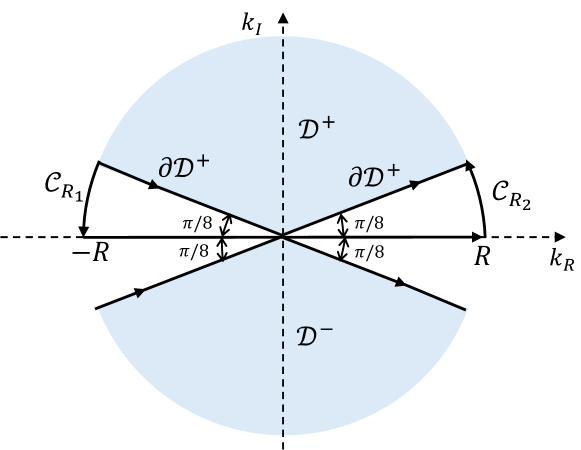
   Figure 1: Contour deformation from the real axis to $\partial\mathcal{D}^{+}$

2. Inserting (31) into the left-hand side of (29) and deforming the real axis to contours in the complex plane $\mathbb{C},$ we have an integral representation along the contour $\partial\mathcal{D}^{+}:=\{k\in\mathbb{C}^{+}:k=\left|k\right|e^{i\theta},\theta=\pi/8\text{ or }7\pi/8\}$ as shown in Figure 2:

   $$\int_{-\infty}^{\infty}e^{ikx}k^{2}\hat{\phi}(k,t)\frac{\mathop{}\!\mathrm{d}k}{2\pi}=\int_{-\infty}^{\infty}e^{ikx-\omega(k)t}\,k^{2}\hat{\phi}_{0}(k)\dfrac{\mathop{}\!\mathrm{d}k}{2\pi}$$ (32)

   $$-\int_{\partial\mathcal{D}^{+}}e^{-\omega(k)t}k^{2}\Big{\{}e^{ikx}\big{[}\tilde{g}_{1}(\omega(k),t)+ik\tilde{g}_{0}(\omega(k),t)$$

   $$\hskip 36.135pt-\hat{p}(k)(\bar{g}_{1}(\omega(k),t)+ik\bar{g}_{0}(\omega(k),t))\big{]}$$

   $$\hskip 36.135pt+e^{ik(L-x)}\big{[}-\tilde{h}_{1}(\omega(k),t)+ik\tilde{h}_{0}(\omega(k),t)$$

   $$\hskip 36.135pt-\hat{p}(k)(-\bar{h}_{1}(\omega(k),t)+ik\bar{h}_{0}(\omega(k),t))\big{]}\Big{\}}\dfrac{\mathop{}\!\mathrm{d}k}{2\pi}$$

3. Employing the transformation $k\to-k$ in (31) which leaves $\omega(k)$ invariant, we eliminate the transforms of unknown boundary values $g_{1},h_{1}$ from $\eqref{eq:state-after-deform-D+}$ and find

   $$\int_{-\infty}^{\infty}e^{ikx}k^{2}\hat{\phi}(k,t)\frac{\mathop{}\!\mathrm{d}k}{2\pi}=\int_{-\infty}^{\infty}e^{ikx-\omega(k)t}\,k^{2}\hat{\phi}_{0}(k)\dfrac{\mathop{}\!\mathrm{d}k}{2\pi}$$ (33)

   $$-\int_{\partial\mathcal{D}^{+}}\dfrac{e^{-\omega(k)t}k^{2}}{e^{ikL}-e^{-ikL}}\Big{\{}2\sin(kx)\big{[}ie^{ikL}\hat{\phi}_{0}(k)$$

   $$\hskip 36.135pt-2k(\tilde{h}_{0}(\omega(k,t))-\hat{p}(k)\bar{h}_{0}(\omega(k),t))\big{]}$$

   $$\hskip 36.135pt+2\sin(k(L-x))\big{[}i\hat{\phi}_{0}(-k)$$

   $$\hskip 36.135pt-2k(\tilde{g}_{0}(\omega(k),t)-\hat{p}(k)\bar{g}_{0}(\omega(k),t)\big{]}\Big{\}}\dfrac{\mathop{}\!\mathrm{d}k}{2\pi}$$

Proof of 1)

Expanding $v_{1}(k,t)$ in (23), we have

$$\hat{\phi}_{t}+\omega(k)\hat{\phi}$$ (34)

$$=-g_{1}(t)-ikg_{0}(t)+e^{-ikL}\left(h_{1}(t)+ikh_{0}(t)\right)$$

$$\quad-\hat{p}(k)\int_{t}^{\infty}e^{\omega(k)(t-\xi)}\big{[}-g_{1}(\xi)-ikg_{0}(\xi)$$

$$\hskip 108.405pt+e^{-ikL}\left(h_{1}(\xi)+ikh_{0}(\xi)\right)\big{]}\mathop{}\!\mathrm{d}\xi.$$

Solving (34), we have the relation (31).

Proof of 2)

Inserting (31) into the left-hand side of (29), we find

$$\int_{-\infty}^{\infty}e^{ikx}k^{2}\hat{\phi}(k,t)\frac{\mathop{}\!\mathrm{d}k}{2\pi}$$ (35)

$$=\int_{-\infty}^{\infty}e^{ikx-\omega(k)t}\,k^{2}\hat{\phi}_{0}(k)\dfrac{\mathop{}\!\mathrm{d}k}{2\pi}$$

$$\quad-\int_{-\infty}^{\infty}e^{ikx-\omega(k)t}\,k^{2}[\tilde{g}_{1}(\omega(k),t)+ik\tilde{g}_{0}(\omega(k),t)$$

$$\qquad-\hat{p}(k)(\bar{g}_{1}(\omega(k),t)+ik\bar{g}_{0}(\omega(k),t))]\dfrac{\mathop{}\!\mathrm{d}k}{2\pi}$$

$$\quad+\int_{-\infty}^{\infty}e^{-ik(L-x)-\omega(k)t}\,k^{2}[\tilde{h}_{1}(\omega(k),t)+ik\tilde{h}_{0}(\omega(k),t)$$

$$\qquad-\hat{p}(k)(\bar{h}_{1}(\omega(k),t)+ik\bar{h}_{0}(\omega(k),t))]\dfrac{\mathop{}\!\mathrm{d}k}{2\pi}$$

The second and third integrals involve unknown functions $g_{1}$ and $h_{1}$; thus, it is hard to evaluate directly. Now, we show that the real axis in the integral can be deformed to specific contours in the complex domain using Lemmas 3 and 4. Then, we will see in Step 3 that the contribution from unknown functions to the integrals vanishes.

To use Lemma 3, we first establish the analyticity of the integrand in (37). It suffices to analyze the analyticity of $\omega(k)=\sqrt{k^{4}+1}$ since the other exponential and polynomial functions of $k$ in (37) are entire functions (analytic everywhere on $\mathbb{C}$). The function $\omega(k)$ is analytic on the entire complex plane excluding the branch cuts $\{\theta=\pm\pi/4\text{ or}\pm 3\pi/4,\left|k\right|\geq 1\}$ where $\omega(k)$ is multi-valued.

Then, we rewrite the integrand as $e^{ikx}G(k;t)$ with

$$G(k;t):=e^{-\omega(k)t}k^{2}\big{[} \tilde{g}_{1}(\omega(k),t)+ik\tilde{g}_{0}(\omega(k),t)$$

$$-\hat{p}(k)(\bar{g}_{1}(\omega(k),t)+ik\bar{g}_{0}(\omega(k),t))\big{]},$$

and find the conditions under which $G(k;t)$ goes to zero as $|k|\to\infty$ to use Lemma 4. The $t$-transforms of boundary values $\tilde{g}_{1},\tilde{g}_{0},\bar{g}_{1},\bar{g}_{0}$ contain the term $\exp[\omega(k)\tau]$ where $\tau<t$. When multiplied by $\exp[-\omega(k)t]$, it follows that $\exp[-\omega(k)(t-\tau)]$ decays exponentially provided that $\text{Re}[\omega(k)]>0$. $\text{Re}[\omega(k)]$ is positive on the complex plane, excluding the branch cuts for $\omega(k)$. Since the polynomial growth of $k^{2}$ will be cancelled by the exponential decay of $\exp[-\omega(k)(t-\tau)]$, $G(k;t)\to 0$ as $\left|k\right|\to\infty$ if $-\pi/4<\theta<\pi/4$ and $3\pi/4<\theta<5\pi/4$.

Figure 2: Contour deformation for (36)

Without loss of generality, let $\mathcal{D}^{+}:=\{k\in\mathbb{C}^{+}:k=|k|e^{i\theta},\pi/8<\theta<7\pi/8\}$, $\partial\mathcal{D}^{+}:=\{k\in\mathbb{C}^{+}:k=\left|k\right|e^{i\theta},\theta=\pi/8\text{ or }7\pi/8\}$ with direction from left to right. In general, $\partial D^{+}$ can be any two rays in $\mathbb{C}^{+}$ with $0<\theta<\pi/4$ and $3\pi/4<\theta<\pi$. Consider a contour $\mathcal{C}=[-R,R]\cup\mathcal{C}_{R_{2}}\cup\partial\mathcal{D}^{+}\cup\mathcal{C}_{R_{1}}$ shown in Figure 2. From Lemma 3 and the analyticity of the integrand $e^{ikx}G(k;t)$ in the domain enclosed by $\mathcal{C}$, we have

$$\int_{\mathcal{C}}e^{ikx}G(k;t)\mathop{}\!\mathrm{d}k$$ (36)

$$= \left(\int_{-R}^{R}+\int_{\mathcal{C}_{R_{2}}}-\int_{\partial\mathcal{D}^{+}}+\int_{\mathcal{C}_{R_{1}}}\right)e^{ikx}G(k;t)\mathop{}\!\mathrm{d}k=0.$$

Taking the limit $R\to\infty$, the integrals over $\mathcal{C}_{R_{1}}$ and $\mathcal{C}_{R_{2}}$ vanish according to Lemma 4. Therefore, $\int_{-\infty}^{\infty}e^{ikx}G(k;t)\mathop{}\!\mathrm{d}k=\int_{\partial\mathcal{D}^{+}}e^{ikx}G(k;t)\mathop{}\!\mathrm{d}k$. Repeat the analysis for the third integral in (35) and replace $\partial\mathcal{D}^{+}$ by $\partial\mathcal{D}^{-}$ that is defined by $\partial\mathcal{D}^{-}:=\{k\in\mathbb{C}^{-}:k=\left|k\right|e^{i\theta},\theta=-\pi/8\text{ or}-7\pi/8\}$, we have:

$$\int_{-\infty}^{\infty}e^{ikx}k^{2}\hat{\phi}(k,t)\frac{\mathop{}\!\mathrm{d}k}{2\pi}$$ (37)

$$=\int_{-\infty}^{\infty}e^{ikx-\omega(k)t}\,k^{2}\hat{\phi}_{0}(k)\dfrac{\mathop{}\!\mathrm{d}k}{2\pi}$$

$$\quad-\int_{\partial\mathcal{D}^{+}}e^{ikx-\omega(k)t}\,k^{2}[\tilde{g}_{1}(\omega(k),t)+ik\tilde{g}_{0}(\omega(k),t)$$

$$\qquad-\hat{p}(k)(\bar{g}_{1}(\omega(k),t)+ik\bar{g}_{0}(\omega(k),t))]\dfrac{\mathop{}\!\mathrm{d}k}{2\pi}$$

$$\quad-\int_{\partial\mathcal{D}^{-}}e^{-ik(L-x)-\omega(k)t}\,k^{2}[\tilde{h}_{1}(\omega(k),t)+ik\tilde{h}_{0}(\omega(k),t)$$

$$\qquad-\hat{p}(k)(\bar{h}_{1}(\omega(k),t)+ik\bar{h}_{0}(\omega(k),t))]\dfrac{\mathop{}\!\mathrm{d}k}{2\pi}.$$

Using the transformation $k\to-k$ in the third integral on the right-hand side of (37), we find that this equation becomes (32).

Proof of 3)

We show that the transforms of unknown boundary values can be eliminated in (32). Note that $\omega(-k)=\omega(k)$, we obtain the following equation from the relation (31) by transforming $k\to-k$:

$$e^{\omega(k)t}\hat{\phi}(-k,t)$$ (38)

$$= \hat{\phi}_{0}(-k)-\tilde{g}_{1}(\omega(k),t)+ik\tilde{g}_{0}(\omega(k),t)$$

$$+e^{ikL}(\tilde{h}_{1}(\omega(k),t)-ik\tilde{h}_{0}(\omega(k),t))$$

$$-\hat{p}(k)\big{[}-\bar{g}_{1}(\omega(k),t)+ik\bar{g}_{0}(\omega(k),t)$$

$$+e^{ikL}(\bar{h}_{1}(\omega(k),t)-ik\bar{h}_{0}(\omega(k),t))\big{]}.$$

In the case that $g_{0}(t),h_{0}(t)$ are given, (38) and (31) become, respectively,

$$e^{\omega(k)t}\hat{\phi}(k,t) =G_{0}(k,t)-(\tilde{g}_{1}-\hat{p}(k)\bar{g}_{1})$$ (39)

$$\hskip 46.97505pt+e^{-ikL}(\tilde{h}_{1}-\hat{p}(k)\bar{h}_{1}),$$

$$e^{\omega(k)t}\hat{\phi}(-k,t) =G_{0}(-k,t)-(\tilde{g}_{1}-\hat{p}(k)\bar{g}_{1})$$

$$\hskip 54.2025pt+e^{ikL}(\tilde{h}_{1}-\hat{p}(k)\bar{h}_{1}),$$

where the known function $G_{0}(k,t)$ is defined by

$$G_{0}(k,t):=\hat{\phi}_{0}(k)-ik(\tilde{g}_{0}-\hat{p}(k)\bar{g}_{0})+ike^{-ikL}(\tilde{h}_{0}-\hat{p}(k)\bar{h}_{0}).$$

Solving (39) for terms containing unknown boundary values, we find

$$\tilde{g}_{1}-\hat{p}(k)\bar{g}_{1} =\frac{1}{\Delta(k)}\left[e^{ikL}G_{0}(k,t)-e^{-ikL}G_{0}(-k,t)\right]$$

$$\hskip 133.69994pt+e^{\omega(k)t}\check{g}_{1},$$

$$\tilde{h}_{1}-\hat{p}(k)\bar{h}_{1} =\frac{1}{\Delta(k)}\left[G_{0}(k,t)-G_{0}(-k,t)\right]+e^{\omega(k)t}\check{h}_{1},$$

where $\Delta(k):=e^{ikL}-e^{-ikL},$ and $\check{g}_{1},\check{h}_{1}$ contain the terms $\hat{\phi}(k,t)$ and $\hat{\phi}(-k,t)$:

$$\check{g}_{1} =-\frac{1}{\Delta(k)}\left[e^{ikL}\hat{\phi}(k,t)-e^{-ikL}\hat{\phi}(-k,t)\right],$$

$$\check{h}_{1} =-\frac{1}{\Delta(k)}\left[\hat{\phi}(k,t)-\hat{\phi}(-k,t)\right].$$

Inserting the expressions for $\tilde{g}_{1}-\hat{p}(k)\bar{g}_{1}$ and $\tilde{h}_{1}-\hat{p}(k)\bar{h}_{1}$ in (32) and simplifying, we find (33) plus the following term that vanishes:

$$\int_{\partial\mathcal{D}^{+}}\left[e^{ikx}k^{2}\check{g}_{1}(k,t)-e^{ik(L-x)}k^{2}\check{h}_{1}(k,t)\right]\dfrac{\mathop{}\!\mathrm{d}k}{2\pi}.$$ (40)

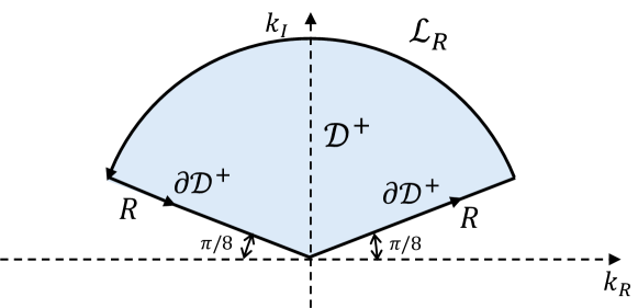
Figure 3: Contour deformation for (41)

To show that the integral (40) vanishes, we analyze the behavior of the integrand as $|k|\to\infty$. $\Delta(k)\sim e^{-ikL}$ since the exponential term $e^{ikL}=e^{(ik_{R}-k_{I})L}$ decays for $k\in\mathbb{C}^{+}$ using the definition $k=k_{R}+ik_{I}$ with $k_{I}>0$. Hence,

$$\check{g}_{1}\sim-\hat{\phi}(-k,t)+e^{ikL}\int_{0}^{L}e^{ik(L-x)}\phi(x,t)\mathop{}\!\mathrm{d}x,\quad|k|\to\infty.$$

$e^{ik(L-x)},e^{ikL}$, and $\hat{\phi}(-k,t)$ all contain the exponential $e^{ik\lambda}$ where $\lambda>0$ that decays in $\mathbb{C}^{+}$. Therefore, $\check{g}_{1}\to 0$ as $|k|\to\infty$ for $k\in\mathbb{C}^{+}$.

Consider a closed curve $\mathcal{L}=\mathcal{L}_{\partial\mathcal{D}^{+}}\cup\mathcal{L}_{R}$, where $\mathcal{L}_{\partial\mathcal{D}^{+}}=\partial\mathcal{D}^{+}\cap\{k:|k|<R\}$ and $\mathcal{L}_{R}=\{k\in\mathcal{D}^{+}:|k|=R\}$, see Figure 3. Note that the pole $k=0$ of $\check{g}_{1}$ is a removable singularity, and we can redefine the value of $\check{g}_{1}$ at $k=0$ to make $\check{g}_{1}$ analytic. From Lemma 3, we have

$$\int_{\mathcal{L}}e^{ikx}k^{2}\check{g}_{1}(k,t)\mathop{}\!\mathrm{d}k$$ (41)

$$= \int_{\mathcal{L}_{\partial\mathcal{D}^{+}}}e^{ikx}k^{2}\check{g}_{1}(k,t)\mathop{}\!\mathrm{d}k+\int_{\mathcal{L}_{R}}e^{ikx}k^{2}\check{g}_{1}(k,t)\mathop{}\!\mathrm{d}k=0.$$

The integral along $\mathcal{L}_{R}$ vanishes as $R\to\infty$ according to Lemma 4 and the fact that $k^{2}\check{g}_{1}\to 0$ as $R\to\infty$ since the exponential decay of $\check{g}_{1}$ cancels the polynomial growth of $k^{2}$. From (41), the integral along $\mathcal{L}_{\partial\mathcal{D}^{+}}$ also goes to zero as $R\to\infty$. Since $\mathcal{L}_{\partial\mathcal{D}^{+}}$ converges to $\partial\mathcal{D}^{+}$ as $R\to\infty$, the contribution from $\check{g}_{1}$ to the integral (40) vanishes. Similarly, the contribution from $\check{h}_{1}$ to the integral (40) also vanishes. Therefore, the value of the integral (40) is zero.

Lastly, we show that (30) holds. Using the definition of $v_{1}$ in (7), the left-hand side of (30) can be expanded as

$$\int_{-\infty}^{\infty}e^{ikx}v_{1}(k,t)\frac{\mathop{}\!\mathrm{d}k}{2\pi}$$ (42)

$$= -\int_{-\infty}^{\infty}e^{ikx}g_{1}(t)\frac{\mathop{}\!\mathrm{d}k}{2\pi}-\int_{-\infty}^{\infty}e^{ikx}ikg_{0}(t)\frac{\mathop{}\!\mathrm{d}k}{2\pi}$$

$$+\int_{-\infty}^{\infty}e^{ik(x-L)}h_{1}(t)\frac{\mathop{}\!\mathrm{d}k}{2\pi}+\int_{-\infty}^{\infty}e^{ik(x-L)}ikh_{0}(t)\frac{\mathop{}\!\mathrm{d}k}{2\pi}$$

$$= -g_{1}(t)\delta(x)-g_{0}(t)\delta^{\prime}(x)$$

$$+h_{1}(t)\delta(x-L)+h_{0}(t)\delta^{\prime}(x-L),$$

where $\delta(\cdot)$ is the Dirac delta function, and $\delta^{\prime}(\cdot)$ is the first derivative of the Dirac delta function. Both $\delta(\cdot)$ and $\delta^{\prime}(\cdot)$ vanish except at the origin, which gives $\eqref{eq:inverse-transform-boundary}$ for $0<x<L$. ∎

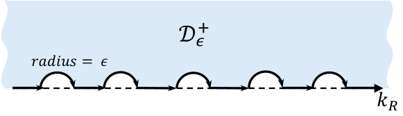
Figure 4: Contour deformation for $\phi(x,t)$

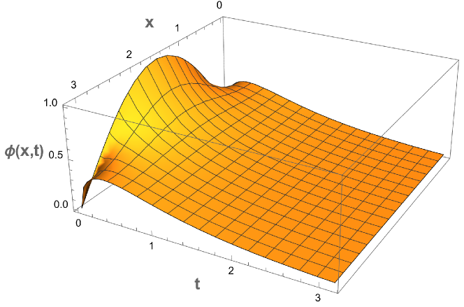
(a) Numerical computation of $\phi(x,t)$ using (28)

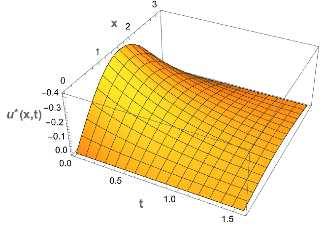
(b) Numerical computation of $u^{*}(x,t)$ using (26)

Figure 5: Numerical computation of the state and control

VI Comparison to existing optimal control

VI-A Equivalent series representations

Consider the heat equation in (1) with $L=\pi$ and homogeneous Dirichlet boundary conditions, i.e., $\phi(0,t)=\phi(\pi,t)=0$. In this setting, an existing optimal control in [6] has a convolution form:

$$u^{*}_{\text{conv}}(x,t)=\int_{0}^{\pi}\left(\Gamma(x-\xi)-\Gamma(x+\xi)\right)\phi(\xi,t)\frac{\mathop{}\!\mathrm{d}\xi}{2\pi}$$ (43)

with

$$\Gamma(x)=\frac{1}{2\pi}\sum_{n=-\infty}^{\infty}\hat{p}(n)e^{inx}.$$

Following [6], the control law (43) is equivalent to the following form:

$$u^{*}_{\text{conv}}(x,t)=\int_{-\pi}^{\pi}\Gamma(x-\xi)\psi(\xi,t)\frac{\mathop{}\!\mathrm{d}\xi}{2\pi}$$ (44)

where $\psi(\xi,t)$ are solutions to the heat equation on $[-\pi,\pi]$ with periodic boundary conditions, initial conditions $\psi_{0}(\xi)=\phi_{0}(\xi)$ if $\xi\in(0,\pi)$ and $\psi_{0}(\xi)=-\phi_{0}(-\xi),u$ if $\xi\in(-\pi,0)$, and the control $v(\xi,t)=u(\xi,t)$ if $\xi\in(0,\pi)$ and $v(\xi,t)=-u(-\xi,t)$ if $\xi\in(-\pi,0)$.

We first rewrite the solution (28) in series representation. This mostly follows from [11, Section 4.2]. Here, we present the main steps. We start by noting that $\Delta(k)=e^{ik\pi}-e^{-ik\pi}=2i\sin(k\pi)$ has simple zeros at $k=n,n\in\mathbb{Z}$. Then for the integral along $\partial\mathcal{D}^{+}$, using Lemma 3 and Lemma 4, we deform it back to the real line with small loops around these roots of radius $\epsilon\to 0$ denoted by $\partial\mathcal{D}_{\epsilon}^{+}$, which is the boundary of $\mathcal{D}_{\epsilon}^{+}$ shown in Figure 4.

Let $f(x,t,k)$ denote the integrand for the integral along $\partial\mathcal{D}^{+}$ in (28). In our case, the small loops around each root have an angular width $\beta=-\pi$. Using Lemma 5, the solution can be rewritten as

$$\phi(x,t) =\int_{-\infty}^{\infty}e^{ikx-\omega(k)t}\,\hat{\phi}_{0}(k)\dfrac{\mathop{}\!\mathrm{d}k}{2\pi}-\int_{\partial\mathcal{D}^{+}_{\epsilon}}f(x,t,k)\dfrac{\mathop{}\!\mathrm{d}k}{2\pi}$$

$$=\int_{-\infty}^{\infty}e^{ikx-\omega(k)t}\,\hat{\phi}_{0}(k)\dfrac{\mathop{}\!\mathrm{d}k}{2\pi}-\mathchoice{{\vbox{\hbox{$\textstyle-$}}\kern-4.86108pt}}{{\vbox{\hbox{$\scriptstyle-$}}\kern-3.25pt}}{{\vbox{\hbox{$\scriptscriptstyle-$}}\kern-2.29166pt}}{{\vbox{\hbox{$\scriptscriptstyle-$}}\kern-1.875pt}}\!\int_{-\infty}^{\infty}f(x,t,k)\dfrac{\mathop{}\!\mathrm{d}k}{2\pi}$$

$$\quad+\frac{\pi i}{2\pi}\sum_{n=-\infty}^{\infty}\text{Residue}[f(x,t,k)]_{k=n}.$$

We first evaluate the principle-value integral and show that it cancels out the first integral. Explicitly expressing $f(x,t,k)$, we have

$$f(x,t,k)=\dfrac{e^{-\omega(k)t}}{\Delta(k)}\big{[}(e^{ik(x+\pi)}-e^{-ik(x-\pi)})\hat{\phi}_{0}(k)$$

$$\hskip 86.72377pt+(e^{ik(\pi-x)}-e^{-ik(\pi-x)})\hat{\phi}_{0}(-k)\big{]}.$$

By rewriting the term with $\hat{\phi}_{0}(-k)$ into another integral and replacing $k$ with $-k$, we have that the integrand in the principle-value integral is the same as the integrand in the first integral. The two integrals cancel out.

Now we evaluate the residue of $f(x,t,k)$ at $k=n$. Note that the function $f(x,t,k)$ is the ratio of two other functions, $f(x,t,k)=h(x,t,k)/\Delta(k)$. Then, the residue of $f(x,t,k)$ at $k=n$ is equal to $h(x,t,n)$ divided by the derivative of $\Delta(k)$ at $k=n$. After some operations, we have

$$\phi(x,t) =-\frac{i}{\pi}\sum_{n=-\infty}^{\infty}e^{inx-\omega(n)t}\int_{0}^{\pi}\sin(n\xi)\phi_{0}(\xi)\mathop{}\!\mathrm{d}\xi$$ (45)

$$=\frac{2}{\pi}\sum_{n=1}^{\infty}\sin(nx)e^{-\omega(n)t}\int_{0}^{\pi}\sin(n\xi)\phi_{0}(\xi)\mathop{}\!\mathrm{d}\xi.$$

(45) is exactly the series expression of $\psi(\xi,t)$ for $\xi\in(0,\pi)$ after substituting (44) into the heat equation with homogeneous periodic boundary conditions.

Repeat similar steps for (26), we have

$$u^{*}(x,t) =-\frac{i}{\pi}\sum_{n=-\infty}^{\infty}\hat{p}(n)e^{inx-\omega(n)t}\int_{0}^{\pi}\sin(n\xi)\phi_{0}(\xi)\mathop{}\!\mathrm{d}\xi$$ (46)

$$=\sum_{n=-\infty}^{\infty}e^{inx}\hat{p}(n)\hat{\psi}(n,t),$$

where $\hat{\psi}(n,t)$ is the discrete Fourier transform of $\psi(x,t)$ in (45). By convolution theorem, $u^{*}(x,t)$ in (46) is equivalent to $u_{\text{conv}}^{*}(x,t)$ in (44).

VI-B Numerical advantages

While we have shown that the integral representation of the state (28) is equivalent to the series representation (45) for homogeneous Dirichlet boundary conditions, the integral representation has numerical advantages. We use Mathematica to directly compute the state and control expressions to compare the numerical properties of the two representations. The initial condition $\phi_{0}(x)=\sin(x)$ is used together with the homogeneous Dirichlet boundary conditions.

Figure 5 shows the numerical computation using the integral representations of the state (28) and the control (26). The infinite series (45) does not converge in the numerical solver, and thus the convolution form (43) cannot be computed without approximation. In contrast, the integral representations (26) and (28) converge in existing numerical integration solvers and can be computed very efficiently. Numerical advantages for complex integral representations have been discussed for general boundary conditions and other types of linear PDEs; see [10] and [15].

VII Conclusions

In this study, we derived the optimal control law for the linear quadratic regulator of the heat equation with general Neumann or Dirichlet boundary conditions using the Fokas method. The control law is given by an integral representation that depends only on the known initial and boundary values. In the special case of homogeneous Dirichlet boundary conditions, we showed that the more general integral representation recovers an existing optimal control law in series representation. The resulting integral representation of the control is easy to compute, whereas the traditional series representation cannot be directly computed without approximation.

Future work includes transforming the integral representation of the optimal control into a feedback form to analyze potential distributed properties. Another direction is to generalize the procedures to derive the control law for other linear PDEs with other types of boundary conditions, such as Robin boundary conditions, where the Fokas method has proven successful. For applications, it is of interest to explore the control design for soft robotics where linear PDEs such as beam equations are used to model the dynamics of soft robots [16].

Appendix

Here, we collect some results from complex analysis.

Lemma 3 (Cauchy’s Theorem [17, Theorem 2.5.2])

If a function $f$ is analytic in a simply connected domain $\mathcal{D}$, then along a simple closed contour $\mathcal{C}$ in $\mathcal{D}$

$$\oint_{\mathcal{C}}f(z)\mathop{}\!\mathrm{d}z=0.$$

Lemma 4 (Jordan’s Lemma [17, Lemma 4.2.2])

Let $\mathcal{C}_{R}$ be a circular arc of radius $R$ centered at the origin and lying on the upper-half complex plane defined by $z=Re^{i\theta}$ with $0\leq\theta_{1}\leq\theta\leq\theta_{2}\leq\pi$. Suppose that on the circular arc $\mathcal{C}_{R}$, we have $f(z)\to 0$ uniformly as $R\to\infty$. Then

$$\lim_{R\to\infty}\int_{\mathcal{C}_{R}}e^{i\lambda z}f(z)\mathop{}\!\mathrm{d}z=0,$$

where $\lambda$ is a real, positive constant.

Remark 4

If $\lambda$ is real and negative, then Jordan’s lemma is still valid, provided that $\mathcal{C}_{R}$ is defined on the lower-half complex plane.

Lemma 5 (​[17, Theorem 4.3.1])

Consider a function $f(z)$ analytic in an annulus centered at $z_{0}$. Let $\mathcal{C}_{\epsilon,\beta[z_{0}]}$ be a circular arc of radius $\epsilon$ and angular width $\beta$, which lies entirely within the annulus centered at $z_{0}:z=z_{0}+\epsilon e^{i\alpha}$, with $\alpha_{0}\leq\alpha\leq\alpha_{0}+\beta$. Suppose $f(z)$ has a simple pole at $z_{0}$. Then

$$\lim_{\epsilon\to 0}\int_{\mathcal{C}_{\epsilon,\beta[z_{0}]}}f(z)\mathop{}\!\mathrm{d}z=i\beta\ \text{Residue}\left[f(z)\right]_{z=z_{0}},$$

where $\text{Residue}\left[f(z)\right]_{z=z_{0}}$ is defined as the value of the coefficient $C_{-1}$ in the Laurent expansion of the function $f(z)=\sum_{n=-\infty}^{\infty}C_{n}(z-z_{0})^{n}$ around the point $z_{0}$.

References

- [1] B. Bamieh, F. Paganini, and M. A. Dahleh, “Distributed control of spatially invariant systems,” IEEE Transactions on automatic control, vol. 47, no. 7, pp. 1091–1107, 2002.
- [2] R. D’Andrea and G. E. Dullerud, “Distributed control design for spatially interconnected systems,” IEEE Transactions on automatic control, vol. 48, no. 9, pp. 1478–1495, 2003.
- [3] N. Motee and A. Jadbabaie, “Optimal control of spatially distributed systems,” IEEE Transactions on Automatic Control, vol. 53, no. 7, pp. 1616–1629, 2008.
- [4] M. R. Jovanovic and B. Bamieh, “On the ill-posedness of certain vehicular platoon control problems,” IEEE Transactions on Automatic Control, vol. 50, no. 9, pp. 1307–1321, 2005.
- [5] C. Langbort and R. D’Andrea, “Distributed control of spatially reversible interconnected systems with boundary conditions,” SIAM journal on control and optimization, vol. 44, no. 1, pp. 1–28, 2005.
- [6] J. P. Epperlein and B. Bamieh, “Spatially invariant embeddings of systems with boundaries,” in 2016 American Control Conference (ACC), pp. 6133–6139, IEEE, 2016.
- [7] J. Arbelaiz, B. Bamieh, A. E. Hosoi, and A. Jadbabaie, “Optimal estimation in spatially distributed systems: how far to share measurements from?,” arXiv preprint arXiv:2406.14781, 2024.
- [8] A. S. Fokas, “A unified transform method for solving linear and certain nonlinear pdes,” Proceedings of the Royal Society of London. Series A: Mathematical, Physical and Engineering Sciences, vol. 453, no. 1962, pp. 1411–1443, 1997.
- [9] A. S. Fokas, A unified approach to boundary value problems. SIAM, 2008.
- [10] A. Fokas and E. Kaxiras, Modern Mathematical Methods for Scientists and Engineers. WORLD SCIENTIFIC (EUROPE), 2023.
- [11] B. Deconinck, T. Trogdon, and V. Vasan, “The method of fokas for solving linear partial differential equations,” SIAM Review, vol. 56, no. 1, pp. 159–186, 2014.
- [12] K. Kalimeris, T. Özsarl, and N. Dikaios, “Numerical computation of neumann controls for the heat equation on a finite interval,” IEEE Transactions on Automatic Control, 2023.
- [13] B. D. Anderson and J. B. Moore, Optimal control: linear quadratic methods. Courier Corporation, 2007.
- [14] J.-W. Wang, H.-N. Wu, and C.-Y. Sun, “Boundary controller design and well-posedness analysis of semi-linear parabolic pde systems,” in 2014 American Control Conference, pp. 3369–3374, IEEE, 2014.
- [15] F. De Barros, M. Colbrook, and A. Fokas, “A hybrid analytical-numerical method for solving advection-dispersion problems on a half-line,” International Journal of Heat and Mass Transfer, vol. 139, pp. 482–491, 2019.
- [16] C. Della Santina, C. Duriez, and D. Rus, “Model-based control of soft robots: A survey of the state of the art and open challenges,” IEEE Control Systems Magazine, vol. 43, no. 3, pp. 30–65, 2023.
- [17] M. J. Ablowitz and A. S. Fokas, Complex variables: introduction and applications. Cambridge University Press, 2003.