Neural quantum states and peaked molecular wave functions: curse or blessing?

Abstract

The field of neural quantum states has recently experienced a tremendous progress, making them a competitive tool of computational quantum many-body physics. However, their largest achievements to date mostly concern interacting spin systems, while their utility for quantum chemistry remains yet to be demonstrated. Two main complications are the peaked structure of the molecular wave functions, which impedes sampling, and large number of terms in second quantised Hamiltonians, which hinders scaling to larger molecule sizes. In this paper we address these issues jointly and argue that the peaked structure might actually be key to drastically more efficient calculations. Specifically, we introduce a novel algorithm for autoregressive sampling without replacement and a procedure to calculate a computationally cheaper surrogate for the local energy. We complement them with a custom modification of the stochastic reconfiguration optimisation technique and a highly optimised GPU implementation. As a result, our calculations require substantially less resources and exhibit more than order of magnitude speedup compared to the previous works. On a single GPU we study molecules comprising up to 118 qubits and outperform the “golden standard” CCSD(T) benchmark in Hilbert spaces of $\sim 10^{15}$ Slater determinants, which is orders of magnitude larger than what was previously achieved. We believe that our work underscores the prospect of NQS for challenging quantum chemistry calculations and serves as a favourable ground for the future method development.

I Introduction

The past decade witnessed an explosive growth of deep learning applications stipulated by a remarkable ability of neural networks to efficiently represent complicated multidimensional probability distributions. To exploit these capabilities in the context of computational quantum many-body physics, Carleo and Troyer pioneered the idea of neural quantum states (NQS), i.e., an efficient representation of a quantum state with a generative neural network [1]. Since its conception the field flourished considerably [2, 3, 4] and now neural quantum states are capable to tackle various problems, including low energy states [5, 6, 7, 8, 9, 10, 11, 12, 13, 14, 15, 16, 17, 18, 19, 20, 21, 22, 23, 24, 25], unitary time evolution [26, 27, 28, 29, 30, 31, 32, 33], open systems [34, 35, 36, 37, 38] and quantum state tomography [39, 40, 41, 42], placing them among state-of-the-art methods of computational quantum many-body physics.

A key advantage of NQS in comparison to alternative methods is the fact that the wave function representation can in principle be efficient irrespective of the interaction graph of the underlying physical system. Therefore, NQS are a promising candidate to tackle the paradigmatic problem of ab initio quantum chemistry to calculate the ground states of molecules in second quantisation. Finding an algorithmic solution to this problem is of outstanding interest, since having access to the ground state of a molecule allows one to deduce most of the physical and chemical properties of the latter. As for any quantum many-body problem, computational approaches are hindered by exponential growth of the Hilbert space with respect to the molecule size, and thus a trade off between the solution accuracy and its efficiency is inevitable. A rich computational toolbox has been elaborated in quantum chemistry, with different methods relying on different approximations, and no method performing universally well across a multitude of molecular systems. Thus, the development of versatile and widely applicable techniques remains a pivotal quest in the field.

However, ever since the first work by Choo et al. [43] on NQS application to ab initio quantum chemistry two outstanding challenges were recognised. First, the molecular ground state wave functions are often of peaked structure, i.e. dominated by few high amplitude components in the computational basis, which constitutes a major obstacle for sampling the Born distribution. Second, molecular Hamiltonians have excessive number of terms, which renders the stochastic estimation of energy highly expensive and poses a formidable challenge of computational nature. A range of subsequent works focused on gradually lifting these limitations by employing better sampling techniques [20], streamlining the energy calculations [22], parallelising the computational load [22, 21], or giving up sampling altogether and resorting to deterministic optimisation [44]. While such collective effort pushed the boundary of what is in principle achievable with NQS to system sizes of several dozens to hundred qubits, competitive energies were so far reported only for systems still amenable to exact diagonalisation. Thus, at its current state the field lacks a compelling evidence suggesting that NQS can both scale up to challenging system sizes and achieve state-of-the-art energies there.

In this work, we supplement NQS quantum chemistry calculations with a set of advances of both conceptual and practical nature aimed at improving its computational performance. As a result, we obtain an optimisation procedure which provides orders of magnitude speedup as compared to the conventional NQS optimisation and yet retains the same accuracy level. Using only a single GPU, we surpass conventional quantum chemistry methods such as CISD, CCSD and CCSD(T) for system sizes that have been previously inaccessible to NQS (118 qubits, $10^{15}$ Slater determinants, $~{}3\cdot 10^{6}$ Hamiltonian terms).

At a high level, we leverage the previously unwelcome peakedness of the wave function. Our contributions include (i) a previously unexplored algorithm for autoregressive sampling without replacement; (ii) two novel approaches to energy evaluation with improved asymptotic complexity; (iii) a modification of the stochastic reconfiguration (SR) optimisation technique tailored to ANQS; (iv) compressed data representation enabling memory and compute efficient GPU implementation.

The remainder of this paper is organised as follows. We provide a relevant background on variational Monte Carlo, quantum chemistry in second quantised formalism and autoregressive neural quantum states in Section II. In Section III we overview at a high-level our contributions, while their technical details are left for Methods. In Section IV we present results of NQS quantum chemistry calculations for a range of molecules beyond exact diagonalisation, showcasing an improved computational performance of the method. Finally, in Section V we conclude our work and indicate directions for future research.

II Background

II.1 Ab initio quantum chemistry

In second quantisation molecular Hamiltonians take the following general form:

$$\hat{H}_{\rm SQ}=\sum_{i,j}t_{ij}(\hat{c}_{i}^{\dagger}\hat{c}_{j}+h.c.)+\sum_{i,j,k,l}V_{i,j,k,l}\hat{c}_{i}^{\dagger}\hat{c}_{j}^{\dagger}\hat{c}_{k}\hat{c}_{l}\,$$ (1)

where fermionic creation and annihilation operators $\hat{c}_{i}^{\dagger},\hat{c}_{i}$ act on a set of $N$ molecular orbitals. In the field of NQS one usually applies the Jordan-Wigner transformation and maps orbitals to a system of $N$ qubits [43, 20, 21]. This produces a Hamiltonian of the following form:

$$\hat{H}_{\rm JW}=\sum_{l=0}^{N_{\rm T}-1}h_{l}\bigotimes_{i=0}^{N-1}\hat{P}_{i}^{(l)},$$ (2)

where $N_{\rm T}$ is the number of terms and $\hat{P}_{i}^{(l)}\in\left\{\hat{I}_{i},\hat{X}_{i},\hat{Y}_{i},\hat{Z}_{i}\right\}$ are Pauli operators acting on the $i$-th qubit. For $n_{\rm e}$ electrons, this Hamiltonian acts on the Hilbert space spanned with $\binom{N}{n_{\rm e}}$ Slater determinants. Each determinant corresponds to $n_{\rm e}$ occupied orbitals and is represented with a basis vector $\ket{\mathbf{x}}=\ket{x_{0}x_{1}\ldots x_{N-1}},\ x_{i}\in\left\{0,1\right\}$. Here the $i$-th orbital is occupied if $x_{i}=1$. The molecular orbitals are usually obtained via the Hartree-Fock procedure. The basis vector $\ket{\mathbf{x}_{\rm HF}}\coloneqq\ket{\underbrace{11\ldots 1}_{n_{\rm e}}\underbrace{0\ldots 0}_{N-n_{\rm e}}}$ represents the Hartree-Fock Slater determinant, which is a mean-field approximation of the true ground state.

The exact diagonalisation of the Hamiltonian, referred to as full configuration interaction (FCI) in quantum chemistry, is clearly restricted by the factorial complexity scaling of Hilbert space size. The traditional quantum chemistry methods trade off accuracy for polynomial complexity and approximate the ground state by choosing a class of trial states. Two most prominent are families of configuration interaction (CI) and coupled cluster (CC) methods, which consider computational spaces spanned by excitations over $\ket{\mathbf{x}_{\rm HF}}$ up to a certain level. Among these methods, CISD, CCSD and CCSD(T) are commonly used, with the latter considered as the de facto “golden standard”.

II.2 Variational Monte Carlo

To approximate the ground state of $\hat{H}$ we use a variational ansatz for the wave function, $\ket{\psi}=\sum_{\mathbf{x}}\psi(\mathbf{x})\ket{\mathbf{x}}$. Here, $\ket{\mathbf{x}{}}$ is a computational basis vector in the Hilbert space of $N$ qubits and $\psi(\mathbf{x})$ is a “black box” function which depends on a set of parameters $\theta$ and returns the quantum state amplitude for $\ket{\mathbf{x}{}}$. We represent $\ket{\psi}$ with a neural network, and refer to the former as neural quantum state (NQS). We numerically optimise the network parameters to minimise the energy expectation value $\langle E\rangle\coloneqq\frac{\braket{\psi}{\hat{H}}{\psi}}{\braket{\psi}{\psi}}$, and thus find the best ground state approximation.

To that end we employ the framework of iterative stochastic optimisation known as variational Monte Carlo (VMC). This approach relies on the fact that quantum expectation values, such as the mean energy $\langle E\rangle$, can be cast in the form of mean values with respect to the Born distribution $p(\mathbf{x})\coloneqq\frac{\left|\psi(\mathbf{x})\right|^{2}}{\sum_{\mathbf{x}}\left|\psi(\mathbf{x})\right|^{2}}$. Hence, they can be estimated efficiently by obtaining a batch $\mathcal{B}$ of $N_{\rm s}$ samples from the distribution $p(\mathbf{x})$. Let $\mathcal{U}\coloneqq\textrm{Unique}(\mathcal{B})$ be the set of unique samples in $\mathcal{B}$ and let $n(\mathbf{x})$ be the occurrence number for the sample $\mathbf{x}$ so that $\sum_{\mathbf{x}\in\mathcal{U}}n(\mathbf{x})=N_{\rm s}$. We call the set of pairs $\Set{\left(\mathbf{x},n(\mathbf{x})\right)}{\mathbf{x}\in\mathcal{U}}$ the sampling statistics. Using the sampling statistics, one estimates the energy of the state as a Monte Carlo expectation value as follows:

$$\langle E\rangle=\mathbb{E}(E_{\rm loc}(\mathbf{x}))\approx\sum_{\mathbf{x}\in\mathcal{U}}E_{\rm loc}(\mathbf{x})\cdot\frac{n(\mathbf{x})}{N_{\rm s}},$$ (3)

where $E_{\rm loc}$($\mathbf{x}$) is the so-called local energy estimator:

$$E_{\rm loc}(\mathbf{x})\coloneqq\sum_{\mathbf{x}^{\prime}:H_{\mathbf{x}\mathbf{x}^{\prime}}\neq 0}\frac{H_{\mathbf{x}\mathbf{x}^{\prime}}\psi(\mathbf{x}^{\prime})}{\psi(\mathbf{x})}.$$ (4)

Similarly, one estimates the gradient of the energy according to Ref. [45]:

$$\begin{gathered}\nabla_{\theta}\langle E\rangle=2\operatorname{Re}\left\{\mathbb{E}\left[E_{\rm loc}(\mathbf{x})\cdot\nabla_{\theta}\ln\psi_{\theta}^{*}(\mathbf{x})\right]\right.\\ \qquad\quad\qquad\qquad-\left.\mathbb{E}\left[E_{\rm loc}(\mathbf{x})\right]\cdot\mathbb{E}\left[\nabla_{\theta}\ln\psi_{\theta}^{*}(\mathbf{x})\right]\right\}.\end{gathered}$$ (5)

This estimate is employed to update the ansatz parameters following the gradient descent rule or any advanced modification thereof [45].

II.3 Autoregressive neural quantum states

The quantum chemistry VMC optimisation is hindered by the fact that the ground state wave functions often have a distinct peaked structure. The dominant contribution comes from the Hartree-Fock Slater determinant, i.e. $p(\mathbf{x}_{\rm HF})$ can be as high as 0.99 or more. As a result, after the initial iterations $\mathbf{x}_{\rm HF}$ constitutes the majority of samples in the batch $\mathcal{B}$. Correspondingly, one needs to resort to large batch sizes $N_{\rm s}$ to explore a non-trivial portion of the Hilbert space and obtain meaningful gradient estimates. This results in a large computational overhead if one optimises an NQS using conventional sampling methods such as Metropolis-Hastings [1, 43].

To mitigate this issue we follow Ref. [20] and employ autoregressive neural quantum states (ANQS). The wave function $\psi(\mathbf{x})$ of an ANQS is a product of single qubit conditional wave functions $\psi_{i}(x_{i}|\mathbf{x}_{<i})$ such that the conditional wave function for the $i$-th qubit depends only on the values of previous $i-1$ qubits:

$$\psi(\mathbf{x})=\prod_{i=0}^{N-1}\psi_{i}(x_{i}|\mathbf{x}_{<i}).$$ (6)

Such a construction enables quick and unbiased sampling from the underlying Born distribution [46, 20]. Importantly, Ref. [20] developed an algorithm which samples the statistics corresponding to a batch of $N_{\rm s}$ samples without producing each sample individually. The complexity of this algorithm is dominated by evaluating amplitudes of only $N_{\rm unq}$ unique basis vectors, where $N_{\rm unq}\coloneqq\left|\mathcal{U}\right|$. This opened the avenue to batch sizes $N_{\rm s}$ as big as $10^{12}$ (with the number of unique samples $N_{\rm unq}\sim 10^{3}\text{--}10^{4}$) and was adopted in subsequent research on ANQS quantum chemistry calculations [21, 22, 23].

III Method advancements

III.1 Sampling without replacement

Both Metropolis-Hastings and conventional autoregressive sampling are examples of so-called sampling with replacement. Such sampling is memoryless, i.e. if $\mathbf{x}$ was obtained as $k$-th sample ($k<N_{\rm s}$), it can still be produced by the ansatz as $k^{\prime}$-th sample, where $k^{\prime}>k$. As a result, the number of obtained unique samples $N_{\rm unq}$ cannot be set in advance; it emerges during sampling. One controls $N_{\rm unq}$ only indirectly by changing the batch size $N_{\rm s}$, and the same value of $N_{\rm s}$ can produce vastly different $N_{\rm unq}$ depending on the probability distribution encoded by the ansatz. The autoregressive statistics sampling of Ref. [20], while being more efficient, also emulates sampling with replacement and hence suffers from the same shortcoming.

It is however desirable to have direct control over $N_{\rm unq}$. First, it defines the computational complexity of both autoregressive statistics sampling and local energy calculations, while $N_{\rm s}$ does not. Second, $N_{\rm unq}$ serves as a direct measure for the Hilbert space portion explored by an ANQS.

To address this issue, we resort to sampling from $p(\mathbf{x})$ without replacement. Such sampling is memoryful, i.e. if $\mathbf{x}$ was obtained as the $k$-th sample, then (i) it can never be obtained in any of subsequent samplings; (ii) the remaining samples are produced from a renormalised probability distribution in which the samples that have already occurred are assigned zero probability. As a result, we obtain a batch of precisely $N_{\rm unq}$ unique samples. Our sampling procedure, based on the algorithm by Kool et al. [47], invokes the ancestral Gumbel top-$K$ trick [48, 49], to autoregressively produce $N_{\rm unq}$ samples without replacement in parallel. We describe further details in Methods and present an ablation study showcasing the computational advantage in the Supplementary Material.

III.2 Streamlined local energy calculations

The calculation of local energies constitutes the central computational bottleneck of NQS quantum chemistry calculations since the number of terms in molecular Hamiltonians grows quartically with the number of orbitals, $N_{\rm T}=\mathcal{O}(N^{4})$ [50]. According to Eq. (4) one has to evaluate ansatz amplitudes for all $\mathbf{x}^{\prime}$ coupled via $\hat{H}$ to sampled $\mathbf{x}\in\mathcal{U}$, i.e. such $\mathbf{x}^{\prime}$ that $H_{\mathbf{x}\mathbf{x}^{\prime}}\neq 0$. This requires $\mathcal{O}(N_{\rm unq}N_{\rm T})$ additional ansatz evaluations, which quickly becomes unwieldy as the system size grows.

To mitigate this problem, we build upon the proposal of Wu et al. [22] and replace the local energy calculation (4) with its computationally cheaper surrogate $E_{\rm loc}^{\rm var}(\mathbf{x})$ which contains contributions only from those $\mathbf{x}^{\prime}$ which belong to the set of unique sampled basis vectors. Hence, for the full energy calculation one requires only the amplitudes of basis vectors in $\mathcal{U}$, which can be computed and stored in memory with $\mathcal{O}\left(N_{\rm unq}\right)$ ansatz evaluations immediately after $\mathcal{U}$ is obtained.

In addition, instead of evaluating the state energy as a Monte Carlo expectation (3) of the local energy, we directly calculate the variational energy of the instantly sampled state:

$$E^{\rm var}=\sum_{\mathbf{x}\in\mathcal{U}}E_{\rm loc}^{\rm var}(\mathbf{x})\cdot\frac{p(\mathbf{x})}{\mathcal{N}},\text{where }\mathcal{N}\coloneqq\sum_{\mathbf{x}\in\mathcal{U}}p(\mathbf{x}).$$ (7)

Here we weigh local energy surrogate values by the renormalised probabilities obtained directly from ansatz, as opposed to weighing them by empirical frequencies $\frac{n(\mathbf{x})}{N_{\rm s}}$. The reason for this is twofold. First, sampling without replacement does not provide any empirical frequencies, but only the unique samples themselves, and thus one cannot use Eq. (3) directly. Second, under such definition, the value calculated via Eq. (7) becomes variational, in that it is always an upper bound for the ground state energy since it corresponds to a physical state spanned by the vectors in $\mathcal{U}$. Hence, in what follows we refer to the value given by Eq. (7) as the variational energy, and to the values of $E_{\rm loc}^{\rm var}(\mathbf{x})$ as the variational (proxy of) local energy.

Improved asymptotic complexity

Although the approach of Ref. [22] reduces the number of ansatz evaluations significantly below $\mathcal{O}(N_{\rm unq}N_{\rm T})$, the number of computational operations required to calculate $E^{\rm var}$ still scales with $N_{\rm T}$. This is because there are $N_{\rm unq}$ values of $E_{\rm loc}^{\rm var}(\mathbf{x})$ to be calculated; to obtain each of them, the authors iterate over $N_{\rm T}$ Hamiltonian terms and calculate the corresponding coupled candidate $\mathbf{x}^{\prime}$. If $\mathbf{x}^{\prime}$ belongs to $\mathcal{U}$, they add the relevant matrix element to the final value. In Ref. [22] checking whether $\mathbf{x}^{\prime}$ belongs to $\mathcal{U}$ is implemented with binary search in $\mathcal{O}(\log N_{\rm unq})$ operations, and thus in total one performs $\tilde{\mathcal{O}}(N_{\rm unq}N_{\rm T})$ operations. Here $\tilde{\mathcal{O}}$ indicates the complexity with omitted logarithmic scaling factors.

In this work we propose two novel methods to evaluate $E^{\rm var}$, which have asymptotic complexity that does not depend on $N_{\rm T}$. Specifically, we split the calculation of $E^{\rm var}$ in two steps. First, we obtain all pairs $(\mathbf{x},\mathbf{x}^{\prime})\in\mathcal{U}\times\mathcal{U}$ which are coupled via the Hamiltonian. We refer to this stage as FindCoupledPairs procedure. Second, we evaluate the matrix elements $H_{\mathbf{x}\mathbf{x}^{\prime}}$ and add the corresponding factors to $E_{\rm loc}^{\rm var}(\mathbf{x})$ and $E_{\rm loc}^{\rm var}(\mathbf{x}^{\prime})$. Our methods focus on improving the asymptotic complexity of FindCoupledPairs. The benchmark implementation we compare with is that of Ref. [22], to which we refer as LoopOverTerms.

When $N_{\rm unq}\ll N_{\rm T}$ the majority of candidate $\mathbf{x}^{\prime}$ will not belong to $\mathcal{U}$. To take advantage of this, our first approach, to which we refer as LoopOverBatch, iterates over each pair $(\mathbf{x},\mathbf{x}^{\prime})\in\mathcal{U}\times\mathcal{U}$ and checks whether there exists a Hamiltonian term coupling $\mathbf{x}$ to $\mathbf{x}^{\prime}$, see Methods for details. This approach brings the complexity of FindCoupledPairs down to $\tilde{\mathcal{O}}(N_{\rm unq}^{2})$.

Our second approach employs an empirical observation that in practice very few pairs $(\mathbf{x},\mathbf{x}^{\prime})$ are actually coupled via the Hamiltonian. Thus, iterating over each element of $\mathcal{U}\times\mathcal{U}$ results in unnecessary computations too. We address this issue by preprocessing $\mathcal{U}$ and reorganising it into a data structure known as prefix tree or simply trie, which we describe in more details in Methods. This data structure allows one to exploit the sparsity of couplings within $\mathcal{U}\times\mathcal{U}$ and substantially speed up FindCoupledPairs. We refer to this implementation of FindCoupledPairs as LoopOverTrie.

III.3 ANQS-tailored stochastic reconfiguration

Standard gradient descent performs poorly in curved parameter spaces, where the learning rate has to be selected carefully so that optimisation does not overshoot narrow ravines. Stochastic reconfiguration (SR) is a gradient postprocessing technique that modifies the energy gradient at every iteration to account for the curvature of underlying variational manifold. To that end, for an ansatz with $N_{\rm p}$ parameters $\{\theta_{p}\}$ one evaluates the so-called $N_{\rm p}\times N_{\rm p}$ quantum geometric tensor (QGT) [51, 52]:

$$S_{pq}=\braket{\partial_{p}\psi}{\partial_{q}\psi}-\braket{\partial_{p}\psi}{\psi}\braket{\psi}{\partial_{q}\psi};\ p,q\in 1..N_{\rm p},$$ (8)

where $\ket{\partial_{p}\psi}\coloneqq\frac{\partial\ket{\psi}}{\partial\theta_{p}}$. QGT captures the local curvature of the parameter space and allows one to “flatten” it by multiplying the energy gradient with an inverse of QGT: $\nabla E\rightarrow S^{-1}\nabla E$.

In VMC applications the overlaps in Eq. (8) are estimated via sampling similarly to Eqs. (3) and (5) [45]. We introduce two modifications to their calculation. First, in the vein of Eq. (7) we evaluate stochastic averages using renormalised probabilities $\frac{p(\mathbf{x})}{\mathcal{N}}$ of unique samples, as opposed to their occurrence numbers. Second, evaluating $\frac{\partial\psi(\mathbf{x})}{\partial\theta_{p}}$ for each $\mathbf{x}$ in $\mathcal{U}$ is computationally heavy, and thus we restrict the set of unique samples used to evaluate $S$. Specifically, we take only first $N_{\rm unq}^{\rm SR}\ll N_{\rm unq}$ unique samples corresponding to the highest probabilities. In all experiments we use $N_{\rm unq}^{\rm SR}=100$ chosen after a study on how $N_{\rm unq}^{\rm SR}$ impacts the achieved variational energies (see Supplementary Material). Apart from a computational benefit, this also seems to numerically stabilise the inversion of $S$, which is performed following the recipes of Refs. [53] and [54].

We use the SR-transformed gradients jointly with the Adam optimiser.We observe that SR substantially boosts the optimisation convergence, i.e. allows achieving lower energies earlier in the optimisation. This observation contrasts with previous reports that cast doubt on the merit of SR for ANQS optimisation [28, 9].

III.4 GPU implementation

Apart from improving the asymptotic complexity of optimisation, we also focus on the practical aspects of its implementation, namely on fully leveraging the inherent massive parallelism of GPUs. We adapt the approach of Wu et al. [22] to store each basis vector $\mathbf{x}$ in a compressed form as a tuple of integers. This leads to a factor of eight memory requirement reduction compared to previous implementations, in which each bit was stored as a one-byte integer. This is critical given our algorithms require simultaneous handling of data structures containing $\mathcal{O}(N_{\rm unq}{}^{2})\gtrsim 10^{9}$ bit vectors of length $N$ (see Supplementary Material).

We advance this method further by implementing all steps of local energy calculation as a sequence of bitwise operations on $\mathbf{x}$ stored in such compressed format. This allows us to replace looping over qubits with vectorised bitwise processor operations, leading to highly accelerated calculations. Specifically, encoding the basis vectors in 64-bit integers speeds up the calculation by a factor of up to 64. As a result, experiments for systems with up to $3\cdot 10^{6}$ Hamiltonian terms required only a single GPU with 24GB of RAM and barely over a second per iteration. This is a substantial reduction in comparison to Refs. [21] and [22] which relied on several GPUs and took dozens of seconds per iteration. In addition, our implementation employs standard tensor algebra routines of PyTorch software library [55] and may be run without any custom CUDA code. We refer the reader to Supplementary Material for an overview of the key aspects of our code.

IV Results

The main implicit assumption behind our approach is that a large enough $N_{\rm unq}$ allows sampling the most important amplitudes as long as the true ground state wave function is peaked enough. In this section we empirically demonstrate the validity of this assumption. We obtain energies that are better than those provided by state-of-the art quantum chemistry methods and/or below chemical accuracy. Equally as importantly, our approach provides an order of magnitude computational speedup compared to existing works.

IV.1 Li2O and BeF2 dissociation curves

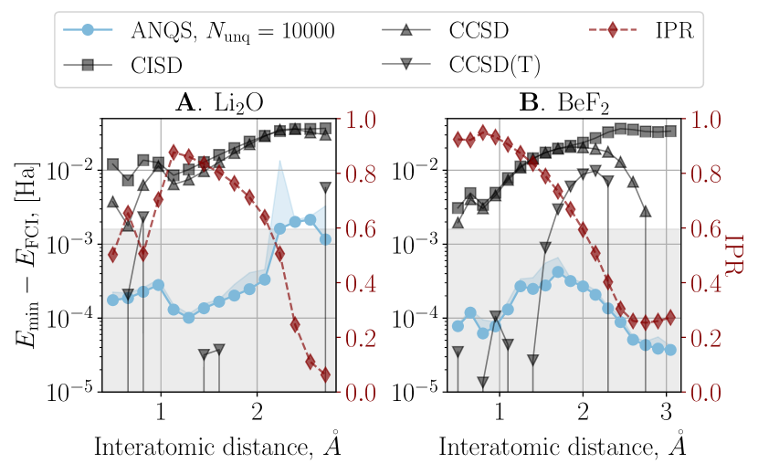
Figure 1: Dissociation curves for Li2O and BeF2 molecules. The grey shaded areas correspond to energy differences within chemical accuracy. The blue shaded areas depict the spread of values from minimum to maximum across seeds. We plot energy differences to the exact diagonalisation (FCI) result ((left y-axis) and ground state IPR (right y-axis) as a function of interatomic distance.

In the first set of experiments we study Li2O and BeF2 molecules both requiring $N=30$ qubits in the minimum basis set STO-3G. These are amongst the largest molecules still amenable to exact diagonalisation. Thus, it is possible to check whether ANQS can achieve chemical accuracy, i.e. whether it can converge to energies within $\Delta E_{\rm chem.acc.}\coloneqq 1.6$ mHa of the true ground state energy $E_{\rm FCI}$. In addition, the unfavourable scaling of local energy calculations is already apparent for these molecules, and in the previous works an optimisation based on the full $E_{\rm loc}$ required an excessive compute time ranging from hours [23] to days [20]. As a result, little progress on extending the ANQS calculations beyond these molecules has been reported so far [21].

We quantify the peakedness of the ground states using the inverse participation ratio (IPR) defined as follows:

$$\mathrm{IPR}\coloneqq\mathop{\mathbb{E}}\left[{p(\mathbf{x})}\right]=\sum_{\mathbf{x}}p(\mathbf{x})\cdot p(\mathbf{x}).$$ (9)

The maximum value of $\mathrm{IPR}$ is 1 and it is achieved when only one basis vector contributes to a wave function, and its minimum is $\frac{1}{2^{N}}$, reached when $\forall\mathbf{x}\ |\psi(\mathbf{x})|=\frac{1}{\sqrt{2^{N}}}$.

For each molecule we explore a range of interatomic distances and for each distance we optimise an ANQS with $N_{\rm unq}=10^{4}$. The minimum achieved variational energies depicted in Fig 1 consistently surpass those obtained by the conventional methods like CISD and CCSD. While ANQS does not always outperform CCSD(T), it is important to remember that the latter can yield unphysical energies below $E_{\rm FCI}$, thus warranting cautious interpretation of such comparison. Crucially, ANQS reliably achieves energies within chemical accuracy for nearly all points on dissociation curves, with a notable exception around 2.4–2.6 Å for Li2O, a region where traditional methods deliver poorer energies too.

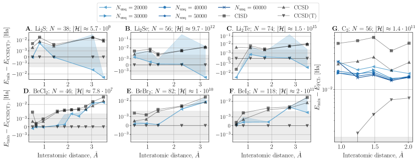
Figure 2: Dissociation curves for bigger molecules as described in the main text. For each molecule we show the number of qubits in the Hamiltonian $N$ as well as the size of the physical Hilbert space. The C2 molecule is considered in cc-pvdz basis set. We plot energy differences to a reference energy as a function of interatomic distance. A–F. The reference energy is obtained with CCSD(T). G. The reference energy is obtained with FCI as reported in [56]. The grey shaded areas correspond to the energy differences within chemical accuracy. The blue shaded areas depict the spread of values from minimum to maximum across seeds.

We also plot the IPR corresponding to each interatomic distance. For Li2O, a higher peakedness generally correlates with the improved optimisation accuracy. However, the accuracy for BeF2 shows a more complicated pattern: it drops with an initial decrease in IPR from approximately 0.9 to 0.75, before improving again as the IPR decreases further to around 0.25. Thus, while the data are compatible with the hypothesis that high peakedness is sufficient for successful optimisation, the overall success may also be influenced by other factors, such as the phase structure of the ground state. Identifying these factors is an important direction for future research.

Finally, let us note that for Li2O molecule with the geometry taken from PubChem database [57] we achieve chemical accuracy on average in 750 seconds. This is 25 times faster compared to Ref. [23], which to the best of our knowledge reported the fastest optimisation for the same molecule so far. The per-iteration time also improves to 0.18 seconds as compared to 8.3 seconds reported in the same work.

IV.2 Further Li and Be compounds

In the next set of experiments we expand the ANQS quantum chemistry calculations to previously challenging system sizes. We obtain dissociation curves for two groups of molecules of increasing size; the first group includes Li2S, Li2Se and Li2Te molecules, while the second consists of BeCl2, BeBr2 and BeI2. We base our selection on their chemical similarity with the already studied Li2O and BeF2: the anion is replaced by a heavier element in the same group 6 (7) of the periodic table. Thus we can systematically scale the number of qubits $N$, the Hilbert space size and the number of terms in Hamiltonian $N_{\rm T}$. We note, however, that since the Hilbert space dimension is $\left|\mathcal{H}\right|{}\coloneqq\binom{N}{n_{\rm e}}$, the largest values of $N$ do not necessarily amount to the largest values of $\left|\mathcal{H}\right|$. For example, the largest studied Hilbert space is that of Li2Te molecule with 74 qubits and $\sim 10^{15}$ Slater determinants, which is three orders of magnitude more than the largest FCI study performed so far [58]. At the same time, the Hilbert space size of BeI2 molecule with 118 qubits is on the order of “mere” $10^{11}$ Slater determinants.

We plot the results of this set of experiments in Fig. 2A–F. We do not have access to FCI energies for these molecules, and thus we plot the difference between the minimum variational energies achieved by ANQS and those obtained with CCSD(T). It can be seen that in the dominant majorities of experiments ANQS outperforms traditional quantum chemistry methods such as CISD and CCSD. When compared to CCSD(T), ANQS results mostly come close to within chemical accuracy, and in some cases surpass them. We consider this as an evidence in favour of the remarkable prospect of ANQS.

IV.3 C2 molecule in cc-pvdz basis set

We also apply ANQS to a paradigmatic strongly correlated system: C2 molecule in the cc-pvdz basis [56]. The results are presented in Fig 2G, where we plot the difference between the lowest energy achieved by ANQS and $E_{\rm FCI}$ as given in Ref. [56]. While we find that increasing $N_{\rm unq}{}$ systematically improves the result, none of $N_{\rm unq}$ values allowed reaching chemical accuracy or surpassing the CCSD(T) energies, even though C2 has a moderate number of qubits (56) and Hilbert space size ($\sim 10^{11}$) as compared to Li and Be compounds studied in the previous section. Nevertheless, an increase in $N_{\rm unq}$ does result in better accuracy, and, starting from $N_{\rm unq}=40000$, ANQS energies surpass those of CISD and CCSD methods. We leave it for future work to explore whether increasing $N_{\rm unq}{}$ further would continue to improve the convergence, or whether the limiting factor is rather the expressivity of the chosen ansatz.

IV.4 Comparison of FindCoupledPairs implementations

In the final set of experiments we benchmark three implementations of the FindCoupledPairs procedure. In Fig. 3A we plot the speedups achieved by LoopOverBatch and LoopOverTrie algorithms compared to the baseline LoopOverTerms implementation. For small values of $N_{\rm unq}$ the LoopOverBatch implementation performs the best, offering up to 10x reduction in time. However, as $N_{\rm unq}$ grows, the advantage of LoopOverBatch becomes less and less pronounced, until it vanishes. For example, for Li2O molecule and $N_{\rm unq}=5\cdot 10^{4}$ it is an order of magnitude slower than the other approaches.

The opposite holds for LoopOverTrie: at low $N_{\rm unq}$ it struggles to compete with LoopOverBatch. However, as both $N_{\rm unq}$ and $N_{\rm T}$ grow, LoopOverTrie becomes more and more advantageous: for example, for Li2Se molecule and $N_{\rm unq}=5\cdot 10^{4}$ it is five times faster than either LoopOverTerms or LoopOverBatch. For Li2Te molecule and the same $N_{\rm unq}$ it demonstrates a tenfold speedup compared to LoopOverTerms.

To accurately estimate the speedup associated with these new techniques, it is important to keep in mind that FindCoupledPairs takes only a part of the compute time in each iteration. The local energy calculation involves three more important subroutines: sampling of $\mathbf{x}$, amplitude evaluation and computing matrix elements $H_{\mathbf{x}\mathbf{x}^{\prime}}$. In Fig. 3B, we show the gains associated with the new FindCoupledPairs algorithms with respect to the total iteration time. In the case of Li2Te molecule and $N_{\rm unq}{}=5\cdot 10^{4}$, the tenfold improvement of LoopOverTrie shrinks down to a factor of four.

In Fig. 4 we plot the fraction of the time spent on each of the four subroutines during the energy calculation. Both for LoopOverTerms and LoopOverBatch the fraction of FindCoupledPairs grows as $N_{\rm unq}$ increases. For the largest molecule (Li2Te) at $N_{\rm unq}=5\cdot 10^{4}$, it amounts for the majority of energy calculation time, while the remaining subroutines take at most 10% of the calculations each. At the same time, FindCoupledPairs implemented as LoopOverTrie constitutes only a third of the energy calculation time, and, more generally, decreases as both $N_{\rm unq}$ and $N_{\rm T}$ grow. Thus, computations related directly to the local energy calculation (as opposed to sampling and amplitude evaluation) are no longer a bottleneck of NQS quantum chemistry.

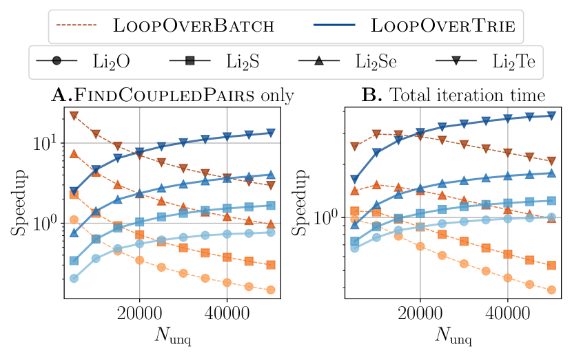
Figure 3: The speedup of LoopOverBatch and LoopOverTrie routines with respect to baseline LoopOverTerms. The speedups are calculated for: A. Only FindCoupledPairs procedure; B. Total iteration time.

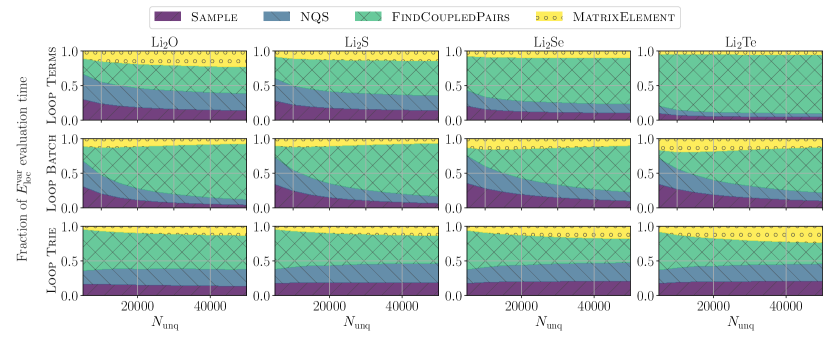
Figure 4: The fraction of the energy evaluation time spent on each of four crucial iteration parts: (i) sampling; (ii) evaluation of amplitudes for basis vectors in $\mathcal{U}$; (iii) finding the coupled pairs $(\mathbf{x},\mathbf{x}^{\prime})$; (iv) calculating the matrix elements between the coupled pairs. Top to bottom rows correspond to different implementations of FindCoupledPairs procedure: LoopOverTerms, LoopOverBatch, LoopOverTrie.

V Discussion

Our results suggest that the peaked ground state wave functions typical for molecules should be not only mitigated in ANQS quantum chemistry calculations, but rather celebrated in certain cases. In particular, it allowed us to leverage an ANQS-specific sampling algorithm which produces the desired number of unique samples. Thus, we were able to focus on a small physically relevant portion of the Hilbert space and greatly accelerate the stochastic estimation of the variational energy by ignoring the contributions from the unsampled part of the Hilbert space. Consequently, we were able to achieve energies that compete with those obtained with the traditional quantum chemistry methods, for computational spaces several orders of magnitude larger than those previously attempted with ANQS.

Remarkably, we even came across certain geometries where the peakedness was less pronounced, and yet focusing only on the sampled subspace still yielded energies within chemical accuracy to the ground state — this was the case, for example, with BeF2. At the same time, we identified cases when our method struggled to reach competitive energies, such as C2. However, it remains to be explored, whether this indicates a general limitation of our method or whether it is due to unrelated issues like bottlenecks in the optimisation [59].

Our results point out further directions for algorithmic improvements and theoretical analysis that would scale up our method. The first observation is that our method is readily amenable to parallelisation across several GPUs. We expect this to enable addressing even larger problem sizes [21, 22], potentially reaching complex organic compounds.

Additionally, the impact of the underlying neural network architecture on the accuracy of optimisation remains a largely unexplored topic. Recently, neural network architectures that are specifically tailored to fermionic systems showed significant promise in application to quantum many-body problems [60, 61], including quantum chemistry  [25, 62]. Combining the enhanced expressivity exhibited by these models with the sampling efficiency of ANQS can potentially give rise to a powerful new approach [63].

We lack understanding on how the choice of $N_{\rm unq}$ influences the learning ability of ANQS. However daunting this question might seem, first steps in similar direction were already made by Astrakhantsev et al. [64]. This work analysed an algorithmic phase transition in the learning dynamics of a variational quantum circuit related to the number of samples produced at each gradient descent step. It is natural to extend these techniques to ANQS optimisation.

Finally, as discussed, the variational energy (7) is an upper bound to the true energy of the NQS, but this upper bound may not be sufficiently tight. The so-called projected energies provide a more accurate estimate [65]. It is to be explored whether ANQS optimisation can be synthesised with this approach to energy calculation for improved optimisation.

Regardless of the actual research path taken, we believe that our work showcases the high promise of ANQS ab initio quantum chemistry calculations beyond the FCI limit. We are optimistic that the ideas presented in this paper, particularly aimed at reducing time and memory requirements of the method, will democratise and facilitate further experiments, thus serving as a fruitful basis for the rapid future progress.

Methods

V.1 Autoregressive sampling without replacement

For sampling without replacement we employ an algorithm developed in Ref. [47] which extends the Gumbel top-$K$ trick [48, 49] to autoregressive probability distributions. This algorithm is not our contribution per se, yet we overview it since it touches upon the ideas previously unexplored within the field of NQS optimisation.

V.1.1 Conventional sampling without replacement

A conventional way to obtain $K$ samples without replacement from a probability distribution $p(\mathbf{x})$ is to produce samples one-by-one and adaptively change the sampled distribution in the following way. Suppose one has sampled without replacement $k-1$ unique samples constituting the set $\mathcal{U}^{(k-1)}$. Then, one obtains the $k$-th unique sample by sampling from the following probability distribution:

$$p^{(k)}(\mathbf{x})=\begin{cases}0,\text{ if }\mathbf{x}\in\mathcal{U}^{(k-1)},\\ \frac{p(\mathbf{x})}{\sum_{\mathbf{x}^{\prime}\not\in\mathcal{U}^{(k-1)}}p(\mathbf{x})}\equiv\frac{p(\mathbf{x})}{1-\sum_{\mathbf{x}^{\prime}\in\mathcal{U}^{(k-1)}}p(\mathbf{x})}\text{ otherwise}.\end{cases}$$ (10)

In other words, one manually removes the probability mass associated with already produced samples and then renormalises the remaining probabilities.

V.1.2 Gumbel top-$K$ trick

The Gumbel top-$K$ trick replaces sequential sampling from $p(\mathbf{x})$ with multiple samplings of another random variable, referred to as the Gumbel noise. The cumulative distribution function of Gumbel noise is given by $F_{\textsc{G}}(g)=e^{-e^{-g}}$. The advantage of this approach is that Gumbel noise sampling can be performed in a parallel fashion. The algorithm proceeds as follows [47]:

1. We obtain a set of i.i.d. samples of Gumbel noise $G_{\mathbf{x}}$, one per each $\mathbf{x}$. This can be achieved by inverse transform sampling as $G=F_{\textsc{G}}^{-1}(U)=-\log\left(-\log U\right)$, where $U\sim\mathrm{Uniform}(0,1)$.

2. We evaluate log-probabilities corresponding to each possible outcome $l_{\mathbf{x}}\coloneqq\log p(\mathbf{x})$, which we further refer to as unperturbed log-probabilities.

3. We calculate the so-called perturbed log-probabilities by adding an Gumbel noise sample to each unperturbed log-probability: $L_{\mathbf{x}}\coloneqq l_{\mathbf{x}}+G_{\mathbf{x}}$.

4. We sort the perturbed log-probabilities in the descending order and take first $K$ $\mathbf{x}$’s corresponding to the highest perturbed log-probabilities as an output of the sampling without replacement algorithm.

To intuitively understand the Gumbel top-$K$ trick, let us suppose we have already selected $k<K$ basis vectors and are now seeking to add the $(k+1)$-st. Let $\mathbf{x}$ and $\mathbf{x}^{\prime}$ be two basis vectors that are not among the $k$ already selected. Let us evaluate the probability of the event that $L_{\mathbf{x}}<g_{{\mathbf{x}^{\prime}}}$, which equals to the probability that $\mathbf{x}^{\prime}$ is selected in this step conditioned on the event that either $\mathbf{x}$ or $\mathbf{x}^{\prime}$ is selected.

This probability is $\Pr(L_{\mathbf{x}}<L_{\mathbf{x}^{\prime}})=\quad\Pr(l_{\mathbf{x}}+G_{\mathbf{x}}<l_{\mathbf{x}^{\prime}}+G_{\mathbf{x}^{\prime}})=\Pr(G_{\mathbf{x}}-G_{\mathbf{x}^{\prime}}<l_{\mathbf{x}^{\prime}}-l_{\mathbf{x}})$. Thus, one seeks the probability for the difference $\Delta G\coloneqq G_{\mathbf{x}}-G_{\mathbf{x}}^{\prime}$ of two independent Gumbel variables to be less than the given value $l_{\mathbf{x}^{\prime}}-l_{\mathbf{x}}$. This probability is given by the value of the CDF $F_{\Delta G}(l_{\mathbf{x}^{\prime}}-l_{\mathbf{x}})$ of the random variable $\Delta G$. It can be calculated to be $F_{\Delta G}(l_{\mathbf{x}^{\prime}}-l_{\mathbf{x}})=\frac{1}{1+e^{-(l_{\mathbf{x}^{\prime}}-l_{\mathbf{x}})}}$. Since $e^{-(l_{\mathbf{x}^{\prime}}-l_{\mathbf{x}})}=\frac{p(\mathbf{x})}{p(\mathbf{x}^{\prime})}$, we obtain that $\Pr({L_{\mathbf{x}}}<{L_{\mathbf{x}^{\prime}}})=\frac{p(\mathbf{x}^{\prime})}{p(\mathbf{x})+p(\mathbf{x}^{\prime})}$. Thus, conditioned on the assumption that either $\mathbf{x}$ or $\mathbf{x}^{\prime}$ is selected, $\mathbf{x}^{\prime}$ is selected with the probability $\frac{p(\mathbf{x}^{\prime})}{p(\mathbf{x})+p(\mathbf{x}^{\prime})}$, whereas $\mathbf{x}$ is selected with the probability $\frac{p(\mathbf{x})}{p(\mathbf{x})+p(\mathbf{x}^{\prime})}$, which is precisely what one expects from sampling without replacement as per Eq. (10).

V.1.3 Autoregressive Gumbel top-$K$ trick

To explain the autoregressive Gumbel top-$K$ sampling let us focus on $K=1$ for simplicity. In this case the ordinary Gumbel top-$K$ trick prescribes evaluating perturbed log-probabilities for all $\mathbf{x}$ and finding the single maximum among them. For $N$ qubits this amounts to $2^{N}$ perturbed log-probabilities and is clearly unfeasible. Hence, the approach of Ref. [47] effectively resorts to a binary search to find the $\mathbf{x}$ corresponding to the maximum of the perturbed log-probabilities.

The authors show that given a vector $\mathbf{x}_{<i}$ the maximum of perturbed log-probabilities of its “children”, i.e. $\max_{\mathbf{x}_{\geq i}}\left(\log p(\mathbf{x}_{<i}\mathbf{x}_{\geq i})+G_{\mathbf{x}_{\geq i}}\right)$ is distributed as $\log p(\mathbf{x}_{<i})+G_{\mathbf{x}_{<i}}\eqqcolon L_{\mathbf{x}_{<i}}$. In other words, the perturbed log-probability of $\mathbf{x}_{<i}$ can serve as an upper bound for the perturbed log-probabilities of its children. Consequently, given $\mathbf{x}_{<i}$ one might estimate the perturbed log-probabilities of $\mathbf{x}_{<i}0$ and $\mathbf{x}_{<i}1$ and keep only that partially sampled vector which has the larger perturbed log-probability. By starting this process with an empty vector $\mathbf{x}_{<0}\equiv\varnothing$ and repeating it iteratively, one obtains the full $\mathbf{x}$ corresponding to the highest perturbed log-probability without exponential growth of complexity.

There is, however, a subtlety. Since the perturbed log-probability of $\mathbf{x}_{<i}$ bounds the perturbed log-probabilities of $\mathbf{x}_{<i}0$ and $\mathbf{x}_{<i}1$ from above, the latter, being sampled at a later stage, should not exceed the value $L_{\mathbf{x}_{<i}}$ obtained at an earlier stage. In other words, sampling of $L_{\mathbf{x}_{<i}0}$ and $L_{\mathbf{x}_{<i}1}$ should be conditioned on the value of $L_{\mathbf{x}_{<i}}$. The authors of Ref. [47] show that the correct conditioned values denoted as $\tilde{L}_{\mathbf{x}_{<i}0}$ and $\tilde{L}_{\mathbf{x}_{<i}1}$ can be obtained by starting with the unconditioned values, finding their maximum $Z\coloneqq\max\left\{L_{\mathbf{x}_{<i}0},L_{\mathbf{x}_{<i}1}\right\}$ and calculating the conditioned ones as $\tilde{L}_{\mathbf{x}_{<i}x_{i}}=-\log\left(\mathrm{e}^{-\tilde{L}_{\mathbf{x}_{<i}}}-\mathrm{e}^{-Z}+\mathrm{e}^{-L_{\mathbf{x}_{<i}x_{i}}}\right)$. As a result, the autoregressive sampling without replacement is described with the following pseudocode:

Algorithm 1 Autoregressive Gumbel top-$K$ sampling

1:function ARGumbelTopK($p_{i}(x_{i}|\mathbf{x}_{<i});\ K$)

2:     # Initialise the set of partially sampled vectors and their (perturbed) log-probabilities.

3:     $\mathcal{UG}\coloneqq\left[\left(\varnothing,0,0\right)\right]$

4:     for $i$ from 0 to $N-1$ do

5:         $\mathcal{UG}^{\prime}\coloneqq\left[\ \right]$

6:         for $(\mathbf{x}_{<i},l_{\mathbf{x}_{<i}},\tilde{L}_{\mathbf{x}_{<i}})$ in $\mathcal{UG}$ do

7:               # Evaluate the unconditioned log-probs

8:              for $x_{i}$ in $\left\{0,1\right\}$ do

9:                  $l_{\mathbf{x}_{<i}x_{i}}\coloneqq l_{\mathbf{x}_{<i}}+\log p_{i}(x_{i}|\mathbf{x}_{<i})$

10:                  $L_{\mathbf{x}_{<i}x_{i}}\coloneqq l_{\mathbf{x}_{<i}x_{i}}+\textsc{Gumbel}(0)$               

11:              $Z\coloneqq\max\left\{L_{\mathbf{x}_{<i}0},L_{\mathbf{x}_{<i}1}\right\}$

12:               # Evaluate the conditioned log-probs

13:              for $x_{i}$ in $\left\{0,1\right\}$ do

14:                  $\tilde{L}_{\mathbf{x}_{<i}x_{i}}~{}\coloneqq~{}-~{}\log\left(\mathrm{e}^{-\tilde{L}_{\mathbf{x}_{<i}}}-\mathrm{e}^{-Z}+\mathrm{e}^{-L_{\mathbf{x}_{<i}x_{i}}}\right)$

15:                  $\mathcal{UG}^{\prime}\texttt{.append}\left((\mathbf{x}_{<i}x_{i},l_{\mathbf{x}_{<i}x_{i}},\tilde{L}_{\mathbf{x}_{<i}x_{i}})\right)$                        

16:         Sort $\mathcal{UG}^{\prime}$ in the descending order of $\tilde{L}_{\mathbf{x}_{<i+1}}$.

17:         $\mathcal{UG}\coloneqq\mathcal{UG}^{\prime}{}[1:K]$.      

18:     $\mathcal{U}\coloneqq$ every $\mathbf{x}$ in $\mathcal{UG}$.

19:     return $\mathcal{U}$

A generalisation to $K>1$ is achieved by retaining top-$K$ (perturbed) log-probabilities during sampling of each qubit, see Ref. [47] for more details. The complexity of Algorithm 1 is $\mathcal{O}\left(N_{\rm unq}\mathcal{C}_{\rm NQS}\right)$, where $\mathcal{C}_{\rm NQS}$ is the complexity of one ansatz evaluation. Importantly, the ansatz evaluations can be parallelised over all $\mathbf{x}_{<i}$ for a given $i$ using batched GPU operations, and the only required loop is over the qubits. As a result, the total complexity of producing $N_{\rm unq}$ samples is comparable to that of evaluating their amplitudes, which is a hallmark of autoregressive ansatzes.

V.2 FindCoupledPairs implementations

V.2.1 Hamiltonian arithmetic

We start our technical consideration of FindCoupledPairs implementation by encoding each Hamiltonian term as follows. We define the bit vector $\mathbf{X}^{(l)}$ encoding the information about the positions of $\hat{X}$ operators in the Hamiltonian term $\hat{P}^{(l)}{}\equiv\bigotimes_{i=0}^{N-1}\hat{P}_{i}^{(l)}$ as follows:

$$X_{i}^{(l)}\coloneqq\begin{cases}1,\text{ if }\hat{P}_{i}^{(l)}=\hat{X};\\ 0,\text{ otherwise. }\end{cases}$$

The bit vectors $\mathbf{Y}^{(l)}$ and $\mathbf{Z}^{(l)}$ are defined in analogous way. Thus, one can store the information about each term as a tuple of four items $\left(h_{l},\mathbf{X}^{(l)},\mathbf{Y}^{(l)},\mathbf{Z}^{(l)}\right)$.

Such representation gives rise to Hamiltonian arithmetic: a set of rules to evaluate $\braket{\mathbf{x}}{\hat{P}^{(l)}}{\mathbf{x}^{\prime}}$ as a sequence of bitwise operations on $N$-bit vectors representing the term and basis vectors:

$$\braket{\mathbf{x}}{\hat{P}^{(l)}}{\mathbf{x}^{\prime}}=\begin{cases}0\text{, if }\mathbf{x}\otimes\mathbf{x}^{\prime}\neq\mathbf{\underline{XY}}^{(l)};\\ \mathrm{e}^{i\phi\left(\mathbf{x}^{\prime},\hat{P}^{(l)}\right)}\text{, otherwise, }\end{cases}$$ (11)

$$\text{where }\phi\left(\mathbf{x}^{\prime},\hat{P}^{(l)}\right)\coloneqq\frac{\pi}{2}\left|\mathbf{Y}^{(l)}\right|+\pi\left|\mathbf{x}^{\prime}\odot\mathbf{\underline{YZ}}^{(l)}\right|,$$

where $\oplus$, $\odot$ and $\otimes$ denote the bitwise OR, AND and XOR operations, respectively, $\left|\mathbf{x}\right|\coloneqq\sum_{i=0}^{N-1}x_{i}$ is the Hamming weight of a $\mathbf{x}$, $\mathbf{\underline{XY}}^{(l)}\coloneqq\mathbf{X}^{(l)}\oplus\mathbf{Y}^{(l)}$ and $\mathbf{\underline{YZ}}^{(l)}\coloneqq\mathbf{Y}^{(l)}\oplus\mathbf{Z}^{(l)}$.

We see that each $\hat{P}^{(l)}$ couples $\mathbf{x}$ to a single $\mathbf{x}^{\prime}$ which can be calculated as $\mathbf{x}^{\prime}=\mathbf{x}\otimes\mathbf{\underline{XY}}^{(l)}$. In other words, a pair ($\mathbf{x}$, $\mathbf{x}^{\prime}$) is coupled by a given Hamiltonian term $\hat{P}^{(l)}$ if $\mathbf{\underline{XY}}^{(l)}$ equals $\mathbf{x}\otimes\mathbf{x}^{\prime}$. The matrix element itself is just a complex exponent with the phase $\phi\left(\mathbf{x}^{\prime},\hat{P}^{(l)}\right)$.

V.2.2 Unique $\mathbf{\underline{XY}}$

Note, however, that in realistic molecular Hamiltonians several $\hat{P}^{(l)}$ might have the same $\mathbf{\underline{XY}}$ representation, i.e. the number of unique $\mathbf{\underline{XY}}^{(l)}$ is less than $N_{\rm T}$. Let us denote the set of all unique $\mathbf{\underline{XY}}^{(l)}$ as $\mathcal{XY}$; the size $\left|\mathcal{XY}\right|$ of this set is still $\mathcal{O}(N_{\rm T})=\mathcal{O}(N^{4})$. For a given $\mathbf{x}$, every implementation of FindCoupledPairs seeks to find a set of $\mathbf{x}^{\prime}$ such that $\mathbf{x}\otimes\mathbf{x}^{\prime}\in\mathcal{XY}$. We denote such set as $\mathcal{SC}_{\mathbf{x}}\coloneqq\Set{\mathbf{x}^{\prime}}{\mathbf{x}\otimes\mathbf{x}^{\prime}\in\mathcal{XY}}$.

V.2.3 LoopOverTerms

The LoopOverTerms implementation can be described with the following pseudocode:

Algorithm 2A Find $\mathcal{SC}_{\mathbf{x}}$ via looping over unique $\mathbf{\underline{XY}}^{(l)}$.

1:function LoopOverTerms($\mathbf{x}$)

2:     $\mathcal{SC}_{\mathbf{x}}\coloneqq\left[\ \right]$

3:     for $\mathbf{\underline{XY}}$ in $\mathcal{XY}$ do

4:         $\mathbf{x}^{\prime}\coloneqq\mathbf{x}\otimes\mathbf{\underline{XY}}$

5:         if $\mathbf{x}^{\prime}$ in $\mathcal{U}$ 

6:              $\mathcal{SC}_{\mathbf{x}}\texttt{.append}\left(\mathbf{x}^{\prime}\right)$               

7:     return $\mathcal{SC}_{\mathbf{x}}$

Invoking LoopOverTerms for all $\mathbf{x}$ in $\mathcal{U}$ results in the time complexity $\mathcal{O}\left(N_{\rm unq}\cdot N_{\rm T}\cdot(\mathcal{C}_{\rm bitop}+\mathcal{C}_{\in\mathcal{U}})\right)$. Here $\mathcal{C}_{\rm bitop}$ is the complexity of a bitwise operation on a pair of basis vectors, which, in principle, is $\mathcal{O}\left(N\right)$. However, with the compressed storing of $N$-bit vectors as tuples of integers discussed in Section III.4 it is possible to reduce the scaling constant by the bit depth of those integers (64 in our case). At the same time, $\mathcal{C}_{\in\mathcal{U}}$ is the complexity of checking whether a candidate vector $\mathbf{x}^{\prime}$ belongs to the batch of sampled unique vectors. In Ref. [22] $\mathcal{U}$ is stored as an ordered table and the checking is performed via binary search; hence $\mathcal{C}_{\in\mathcal{U}}=\mathcal{O}\left(\log N_{\rm unq}\right)$. However, implementing binary search posed a significant challenge for our GPU-based implementation. Hence, in Supplementary Material we propose an alternative approach with similar asymptotic complexity.

V.2.4 LoopOverBatch

The pseudocode for LoopOverBatch is as follows:

Algorithm 2B Find $\mathcal{SC}_{\mathbf{x}}$ via looping over $\mathcal{U}$.

1:function LoopOverBatch($\mathbf{x}$)

2:     $\mathcal{SC}_{\mathbf{x}}\coloneqq\left[\ \right]$

3:     for $\mathbf{x}^{\prime}$ in $\mathcal{U}$ do

4:         $\mathbf{\underline{XY}}\coloneqq\mathbf{x}\otimes\mathbf{x}^{\prime}$

5:         if $\mathbf{\underline{XY}}$ in $\mathcal{XY}$ 

6:              $\mathcal{SC}_{\mathbf{x}}\texttt{.append}\left(\mathbf{x}^{\prime}\right)$               

7:     return $\mathcal{SC}_{\mathbf{x}}$

Invoking LoopOverTerms for all $\mathbf{x}$ in $\mathcal{U}$ results in the time complexity $\mathcal{O}\left(N_{\rm unq}^{2}(\mathcal{C}_{\rm bitop}+\mathcal{C}_{\in\mathcal{XY}})\right)$. Similarly to LoopOverTerms $\mathcal{C}_{\in\mathcal{XY}}{}=\mathcal{O}\left(\log N_{\rm T}\right)$ is the complexity of checking whether each calculated $\mathbf{\underline{XY}}$ belongs to $\mathcal{XY}$. To implement this check in $\ll\mathcal{O}(N_{\rm T})$ operations for each pair, we create an ordered data structure that lists both the $(\mathbf{x},\mathbf{x}^{\prime})$ pairs and the Hamiltonian terms encoded as bit vectors in a way enabling rapid lookup, as further explained in the Supplementary.

V.2.5 Prefix tree

Prefix tree (also known as trie) is a data structure used to store a set of bit vectors (or more generally strings over some alphabet) in a compressed way. Suppose one has to store two strings $abcd$ and $abce$. Both strings share the same prefix $abc$; to avoid keeping redundant information, one might just store the prefix $abc$, two possible endings $d$ and $e$ and the way the endings are connected to the prefix. The prefix tree develops this idea further and applies it to all possible prefixes in a set of strings as illustrated in Fig. 5. From a more formal perspective, prefix tree is a directed tree, where the root node corresponds to the “start of a string” symbol, ordinary nodes contain string symbols, and every path in the tree from the root to a leaf represents a particular string in the set.

V.2.6 Prefix tree construction

Algorithm 3 presents a pseudocode to construct a prefix tree from a set of unique bit vectors. We store the tree $\mathcal{T}$ as a list of nodes representing unique prefixes. We presume that each node is a data structure with three fields: value, storing $x_{i}$; parent, storing the reference to a parent node at the previous level; and array of two references children to children nodes at the next level. By default, the references are set to None indicating that the link between the node and its parent/children has not been established yet. The prefix $\mathbf{x}_{<i}$ of a node can be reconstructed by traversing the prefix tree up via parent references.

Algorithm 3 Constrution of prefix tree

1:function ConstructPrefixTree($\mathcal{U}$)

2:     $\mathcal{T}\coloneqq\left[\ \right]$

3:     $\mathcal{T}\texttt{.append}\left(\textsc{Node}(\texttt{value}=\varnothing)\right)$

4:     for $\mathbf{x}$ in $\mathcal{U}$ do

5:         $\texttt{current\_node}\coloneqq\mathcal{T}[0]$

6:         for $i$ from 0 to $N-1$ do

7:              if $\texttt{current\_node}.\texttt{children}[x_{i}]$ $=$ None 

8:                  $\texttt{new\_node}\coloneqq~{}\textsc{Node}(\text{{value}=$x_{i}$})$

9:                  $\texttt{new\_node}.\texttt{parent}\coloneqq\texttt{current\_node}$

10:                  $\texttt{current\_node}.\texttt{children}[x_{i}]\coloneqq\texttt{new\_node}$

11:                  $\mathcal{T}\texttt{.append}\left(\texttt{new\_node}\right)$               

12:              $\texttt{current\_node}\coloneqq\texttt{current\_node}.\texttt{children}[x_{i}]$               

13:     return $\mathcal{T}$

V.2.7 LoopOverTrie

As discussed, Algorithm 2B evaluates $\mathbf{x}{}\otimes\mathbf{x}^{\prime}{}$ for each pair of unique basis vectors and then checks whether the result belongs to $\mathcal{XY}$. This requires looping over every bit in $\mathbf{x}$ and $\mathbf{x}^{\prime}$. Importantly, during this loop, Algorithm 2B does not try to check whether a partial XOR of $\mathbf{x}$ and $\mathbf{x}^{\prime}$ is valid, i.e. whether it might be a prefix of any $\mathbf{\underline{XY}}$ in $\mathcal{XY}$. Such approach results in unnecessary calculations, since it might become apparent early in the loop that $\mathbf{x}$ and $\mathbf{x}^{\prime}$ cannot be coupled by any term in $\hat{H}$.

In Algorithm 2C we address this issue and remove the “futil” pairs $(\mathbf{x}_{<i},\mathbf{x}^{\prime}_{<i})$ from consideration as early as possible. To that end, we store both $\mathcal{U}$ and $\mathcal{XY}$ as prefix trees, which we denote as $\mathcal{T}^{\mathcal{U}}$ and $\mathcal{T}^{\mathcal{XY}}$ correspondingly. For a given $\mathbf{x}$, we traverse the prefix tree $\mathcal{T}^{\mathcal{U}}$ level-by-level and keep only those paths which correspond to a valid prefix of the same length in $\mathcal{T}^{\mathcal{XY}}$. Note that checking whether $\mathbf{\underline{XY}}_{<i}$ belongs to $\mathcal{T}^{\mathcal{XY}}$ does not require any search operations. Instead, since each prefix $\mathbf{\underline{XY}}_{<i}$ is built sequentially starting from the root, one only needs to examine whether the node corresponding to $\mathbf{\underline{XY}}_{<i-1}$ has a child corresponding to $x_{i}\otimes x^{\prime}_{i}$.

Algorithm 2C Find $\mathcal{SC}_{\mathbf{x}}$ via prefix tree.

1:function LoopOverTrie($\mathbf{x}$)

2:     $\mathcal{T}^{\mathcal{U}}\coloneqq\textsc{ConstructPrefixTree}(\mathcal{U})$

3:     $\mathcal{T}^{\mathcal{XY}}\coloneqq\textsc{ConstructPrefixTree}(\mathcal{XY})$

4:     # Initialise a set of coupled $\mathbf{x}^{\prime}_{<i}$ and corresponding $\mathbf{\underline{XY}}_{<i}$.

5:     $\mathcal{SCXY}_{\mathbf{x}}\coloneqq\left[(\mathcal{T}^{\mathcal{U}}[0],\mathcal{T}^{\mathcal{XY}}[0])\right]$

6:

7:     for $i$ from 0 to $N-1$ do

8:         $\mathcal{SCXY}_{\mathbf{x}}^{\prime}\coloneqq\left[\ \right]$

9:

10:         for (u_node, xy_node) in $\mathcal{SCXY}_{\mathbf{x}}$ do

11:              for $x_{i}^{\prime}$ in $\left\{0,1\right\}$ do

12:                  $\texttt{new\_u\_node}\coloneqq\texttt{u\_node}.\texttt{children}[x_{i}^{\prime}]$

13:                  $\texttt{new\_xy\_node}\coloneqq\texttt{xy\_node}.\texttt{children}[x_{i}\otimes x_{i}^{\prime}]$

14:

15:                  if new_u_node $\neq$ None and new_xy_node $\neq$ None 

16:                       $\mathcal{SCXY}_{\mathbf{x}}^{\prime}\texttt{.append}\left((\texttt{new\_u\_node},\ \texttt{new\_xy\_node}{})\right)$

17:                  else

18:                       continue                                          

19:         $\mathcal{SCXY}_{\mathbf{x}}\coloneqq\mathcal{SCXY}_{\mathbf{x}}^{\prime}$      

20:     Reconstruct $\mathcal{SC}_{\mathbf{x}}$ from every u_node in $\mathcal{SCXY}_{\mathbf{x}}$.

21:     return $\mathcal{SC}_{\mathbf{x}}$

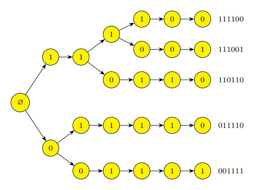
Figure 5: Prefix tree for a set of five bit vectors $\left\{001111,011110,110110,111001,111100\right\}$. One can see that, for example, the strings $110110$ and $111001$ are encoded by the same first two levels of the prefix tree, while the remaining levels are different for them.

V.2.8 LoopOverTrie complexity

To conclude the discussion of LoopOverTrie, let us consider its worst case computational complexity. The worst case corresponds to the situation when all $\mathbf{x}$ in $\mathcal{U}$ are coupled to each other and no paths are dropped during the traversal of $\mathcal{T}^{\mathcal{U}}$. Hence, starting from some level we have $N_{\rm unq}{}$ paths. Consequently, the number of operations required to traverse through $N$ levels of $\mathcal{T}^{\mathcal{U}}$ is bounded from above by $\mathcal{O}(N\cdot N_{\rm unq})$. Since we invoke LoopOverTrie for each $\mathbf{x}$ in $\mathcal{U}$, the total complexity of FindCoupledPairs becomes $\mathcal{O}(N\cdot N_{\rm unq}^{2})$. Thus, we recover the complexity of all-to-all coupling Algorithm 2B, assuming that $\mathcal{C}_{\rm bitop}=\mathcal{O}(N)$.

The above discussion leads us to expect LoopOverTrie to be at least as fast as LoopOverBatch. However, this is not always the case in practice, as evident from Fig. 3. This is because LoopOverTrie requires explicit looping over $N$ levels of prefix trees, and thus loses the benefits of the compressed basis vector storing. Nevertheless, for large systems efficient exploitation of coupling sparsity outweighs this disadvantage, and LoopOverTrie does demonstrate practical speedups.

V.3 Experimental particulars

V.3.1 General setup

All experiments were performed on a single NVIDIA RTX A5000 GPU with 24 GB of RAM. For a given molecule and its geometry, we obtain the qubit Hamiltonian with OpenFermion software library [66], which uses PySCF [67] and Psi4 [68] quantum chemistry packages as underlying backends to calculate one- and two-body integrals. We study all molecules in the minimal basis set STO-3G, unless specified otherwise. For each molecule we obtain the maximum set of symmetries and ensure symmetry-aware sampling as described in Ref. [23]. For each geometry we run calculations using three different seeds of the underlying pseudorandom number generator. When discussing achieved energies we report the minimum value obtained across seeds unless specified otherwise. For other metrics we report the mean value. We invite the reader interested in specific values of the hyperapameters and/or reproducing the experimental results to explore the supplementary GitHub repository [69].

V.3.2 Ansatz architecture

We employ an ANQS architecture which represents each conditional wave function with two real-valued subnetworks, separately encoding absolute value $\log\left|\psi\right|$ and phase $\varphi$ of an amplitude $\psi=\mathrm{e}^{\log\left|\psi\right|+\mathrm{i}\varphi}$. This allows us to perform SR gradient postprocessing without worrying about numerical instability issues arising with complex-valued subnetworks.

Each ANQS subnetwork is a multi-layer perceptron with two hidden layers of width 64. There is a residual connection adding the output of the first hidden layer to the output of the second before the second layer is activated. The hidden layers are activated with the hyperbolic tangent function, while no elementwise activation is applied to the last layer. Instead, we apply a global activation to the last layer which we describe below.

V.3.3 Local pruning strategy

At each level of the autoregressive tree, we mask unphysical nodes (set their probabilities to zero) as described in Barrett at al. [20]. We do not use more sophisticated masking strategies proposed in our earlier work [23]. This is due to our lack of understanding how to reconcile discarding the samples required by these strategies with autoregressive sampling without replacement.

V.3.4 Grouping qubits into qudits

We alleviate the expressivity restriction brought about by our masking strategy by grouping multiple qubits into qudits and sampling the latter. The number $N_{\rm\frac{qubit}{qudit}}$ of qubits per qudit is a hyperparameter, which we chose to equal 6 as a result of a study described in Supplementary Material . If $N$ is not a multiple of $N_{\rm\frac{qubit}{qudit}}$, the last subnetwork groups the remaining $\left(N\mod N_{\rm\frac{qubit}{qudit}}\right)$ qubits into a last qudit. A further advantage of grouping qubits into qudits is faster sampling and amplitude evaluation, which we also cover in Supplementary Material.

V.3.5 Global activation

Once the log-amplitude subnetwork produces unnormalised values for $\log\left|\psi\left(x_{i}|\mathbf{x}_{<i}\right)\right|$, we apply a global activation function to them. Specifically, we shift them by their average, i.e. $\log\left|\psi\left(x_{i}|\mathbf{x}_{<i}\right)\right|\rightarrow\log\left|\psi\left(x_{i}|\mathbf{x}_{<i}\right)\right|-\sum_{x_{i}}\log\left|\psi\left(x_{i}|\mathbf{x}_{<i}\right)\right|$, where the summation over $x_{i}$ includes all possible $2^{N_{\rm\frac{qubit}{qudit}}}$ values of $i$-th qudit. In our preliminary experiments we observed empirically that such global activation improves the optimisation convergence.

Supplementary material: Neural quantum states and peaked molecular wave functions: curse or blessing?

This supplementary consists of two main parts. In Section S1 we cover the ablation studies mentioned in the main text. Namely, we ablate autoregressive sampling without replacement, grouping qubit into qudits and stochastic reconfiguration. The remaining sections are dedicated to GPU implementation of $E_{\rm loc}^{\rm var}$ calculation using primitives of PyTorch software library [55]. In Section S2 we introduce a toy problem which we use as illustration in the remaining sections. In Section S3 we cover the general principles behind our implementation: contiguous storing of information and pointer arithmetic. In Section S4 we explain implementations of LoopOverBatch and MatrixElement. In Section S5 we discuss how to perform prefix tree operations on a GPU and provide implementation for LoopOverTrie. Finally, the considered higher-level routines require auxiliary lower-level functions not readily available in PyTorch, and we overview their implementation in Section S6.

S1 Ablation studies

S1.1 Autoregressive Gumbel sampling

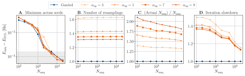
Figure S1: An ablation study comparing Gumbel sampling to adaptive statistics sampling strategies for several values of $\alpha_{\rm up}$. A. Achieved energy differences with respect to $E_{\rm FCI}$; the grey shaded area corresponds to the energy differences within chemical accuracy of 1.6 mHa. B. Number of resamplings required to obtain the desired number of unique samples. C. Ratio of the actual number of unique samples produced during the last resampling to the desired $N_{\rm unq}$. D. Slowdown in the total iteration time brought by adaptive sampling as compared to the Gumbel sampling iteration time.

In this ablation study we compare autoregressive Gumbel sampling to adaptive autoregressive statistics sampling. As discussed in the main text, autoregressive Gumbel sampling is advantageous due to its ability to produce the number of unique samples $N_{\rm unq}$ exactly as specified by the user. However, it is possible to obtain the desired number of samples at every iteration with the conventional autoregressive statistics sampling [20, 23] too. To that end one has to resort to adaptive sampling: if the number of produced unique samples is less than $N_{\rm unq}$, then one increases $N_{\rm s}$ according to some batch size schedule and samples again.

Specifically, we consider the following adaptive scheme: if the number of produced unique samples is less than $N_{\rm unq}$, we increase $N_{\rm s}$ by a factor of $\alpha_{\rm up}$ and sample again. As soon as the number of obtained unique samples exceeds $N_{\rm unq}$, we stop sampling and select the first $N_{\rm unq}$ unique samples with the highest probabilities $p(\mathbf{x})$ produced by the ansatz. In addition, to avoid soaring values of $N_{\rm s}$, we decrease the batch size by a factor of $\alpha_{\rm down}=2$ before the first sampling attempt of each iteration. One might consider various other adaptive sampling approaches, however this remains outside the scope of this paper.

For our benchmark we optimise an ANQS corresponding to the Li2O molecule for $2\cdot 10^{4}$ iterations using plain Adam optimiser across a range of $N_{\rm unq}$. We choose five possible values of $\alpha_{\rm up}=\left\{3,5,7,9\right\}$. In addition, we run calculations using only autoregressive Gumbel sampling.

The results of optimisation are presented in Fig. S1. One can see in Fig. S1A that the energy errors achieved by all sampling strategies are similar to a good degree of accuracy, with no sampling scheme having a competitive edge over others. At the same time all sampling approaches apart from Gumbel require on average more than one sampling per iteration as displayed in Fig. S1B. Evidently, the number of resamplings decreases as $\alpha_{\rm up}$ grows, since it takes fewer attempts to reach higher values of $N_{\rm s}$. However, this comes at a cost of increased computational burden as shown in Fig. S1C: the actual number of unique samples produced during each successful sampling attempt is larger than $N_{\rm unq}$ for all adaptive sampling strategies. As a result, every adaptive sampling scheme increases iteration time with respect to Gumbel sampling as presented in Fig. S1D. Notably, lower values of $\alpha_{\rm up}$ slow down the computation more, since restarting sampling multiple times is more expensive than producing more unique samples as long as the batch of unique samples fits in the GPU RAM.

Finally, let us note that while the slowdowns displayed in Fig. S1D are rather moderate, this is mainly due to sampling taking less than 15% of the total iteration time as shown in Fig. 4 of the main text. However, we expect the advantage of Gumbel sampling to become more pronounced for larger molecules, with sampling taking a larger part of iteration time.

S1.2 Grouping qubits into qudits

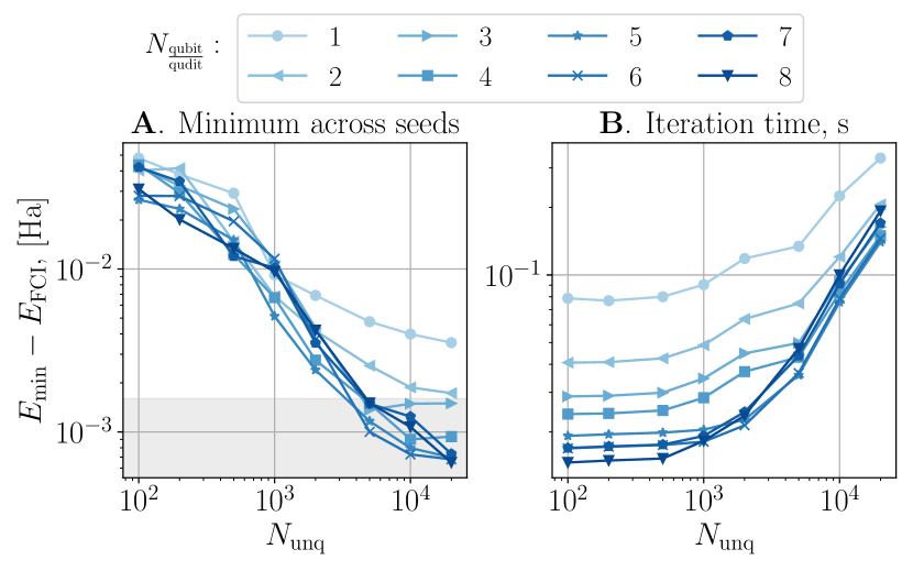
$N_{\rm\frac{qubit}{qudit}}$	$N_{\rm p}$
1	317,048
2	161,528
3	112,288
4	97,128
5	85,376
6	91,648
7	118,408
8	148,224

Figure S2: An ablation studying the impact of grouping qubits into qudits. A. Achieved energy differences with respect to $E_{\rm FCI}$; the grey shaded area corresponds to the energy differences within chemical accuracy of 1.6 mHa. B. Iteration time averaged across seeds.

In this ablation study we investigate the impact of grouping qubits into qudits. Similarly to above, we optimise the ANQS representing the Li2O molecule for $2\cdot 10^{4}$ iterations without resorting to SR. We consider every possible value of $N_{\rm\frac{qubit}{qudit}}$ from 1 to 8 and show the results in Fig. S2. One can see in Fig. S2A that low values of $N_{\rm\frac{qubit}{qudit}}$ such as 1 and 2 consistently perform the worst in terms of the achieved energy error, even though they have the largest number of parameters as shown in the table in Fig. S2. This is in agreement with previous reports indicating that masking conditional wave functions required for correct symmetry-aware sampling reduces the expressivity of an ANQS [70, 71, 23]. At the same time, increasing $N_{\rm\frac{qubit}{qudit}}$ results in steady improvement of the achieved accuracy, with $N_{\rm\frac{qubit}{qudit}}{}=5,6$ providing the best energies at $N_{\rm unq}=20000$. Importantly, these values of $N_{\rm\frac{qubit}{qudit}}{}$ also result in the least time spent on sampling and amplitude evaluation as depicted in Fig. S2. This is due to the fact that larger $N_{\rm\frac{qubit}{qudit}}$ amount to fewer conditional wave functions $\psi(x_{i}|\mathbf{x}_{<i})$ constituting the ansatz (the number of conditional wave functions is given by $\left\lceil\frac{N}{N_{\rm\frac{qubit}{qudit}}{}}\right\rceil$).

Similar regularities were obtained in our preliminary experiments on other molecules. As a result, we chose $N_{\rm\frac{qubit}{qudit}}{}=6$ for all numerical experiments described in the main text.

S1.3 Stochastic reconfiguration

In the final ablation study we investigate how SR affects the accuracy and computational efficiency of ANQS quantum chemistry calculations. Prior to comparing the optimisation with and without SR, we select the optimal hyperparameter $N_{\rm unq}^{\rm SR}$. Similarly to the previous ablation studies, we consider the Li2O molecule and run ANQS optimisation with different values of $N_{\rm unq}^{\rm SR}{}\in\left\{1,10,25,50,100,200\right\}$; as well we run optimisation instances which do not employ stochastic reconfiguration. We run each optimisation configuration with 5 different seeds of the underlying pseudorandom number generator and in each run we measure the minimum achieved energy.

In Fig. S4A and Fig. S4B we show, respectively, the minimum and median achieved energies across the five seeds. Generally, larger values of $N_{\rm unq}^{\rm SR}$ result in lower achieved energies, with $N_{\rm unq}^{\rm SR}=100$ providing the best energy starting from $N_{\rm unq}=10^{3}$. Rather surprisingly, stochastic reconfiguration does not always translate into the improved convergence: for example, $N_{\rm unq}^{\rm SR}=1$ and $N_{\rm unq}^{\rm SR}=25$ provide worse energies than purely Adam-based optimisation. The larger value of $N_{\rm unq}^{\rm SR}$, namely 200, does not result in better energies either, even though one might naïvely expect it to provide a more accurate estimate of the metric tensor $S$. We attribute such behaviour to sharp singular spectrum of $S$ typical for NQS. A larger $N_{\rm unq}^{\rm SR}$ gives rise to multiple, very small singular values, introducing numerical noise which affects the accuracy of the inversion of $S$.

In Fig. S4 we show exemplary training curves for optimisation of the Li2O molecule with $N_{\rm unq}=10^{4}$. Specifically, we show how $E^{\rm var}$ changes with the iteration number (Fig. S4A) and elapsed time (Fig. S4B) for two optimisations run (i) with $N_{\rm unq}^{\rm SR}=100$ and (ii) without SR. It can be seen that the SR-driven optimisation achieves lower energies substantially earlier. However, once the required iteration time is taken into account, the optimisation performed without SR catches up and might eventually achieve similar energies in a similar time. The optimal strategy could therefore be to start the training with SR and switch it off as soon as the iterations “break through” to energies below a certain threshold.

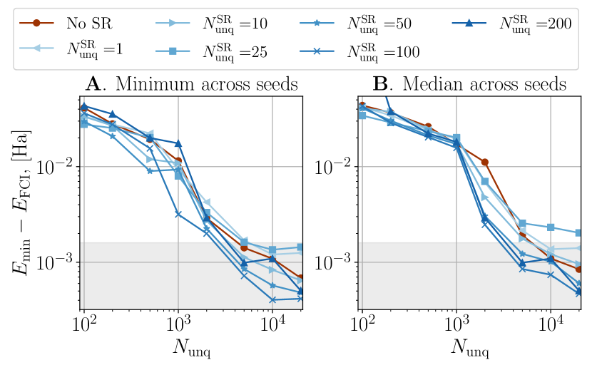
Figure S3: Impact of hyperparameter $N_{\rm unq}^{\rm SR}$ in stochastic reconfiguration. We plot the achieved energy differences with respect to $E_{\rm FCI}$; the grey shaded area corresponds to energy differences within the chemical accuracy of 1.6 mHa. Figures A and B show minimum and median statistics calculated across five seeds respectively.

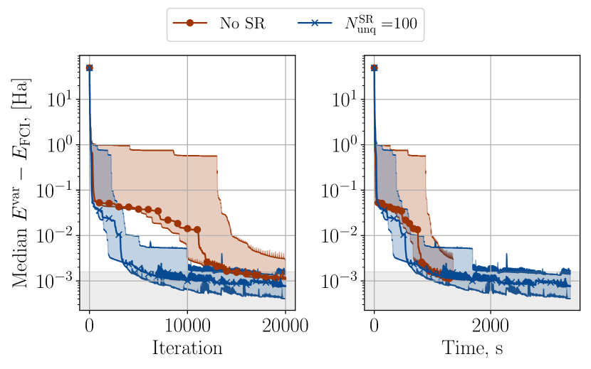
Figure S4: Example training curves for Li2O molecule at $N_{\rm unq}=10000$. We show median energy differences to the exact diagonalisation (FCI) result as a function of (A) iteration number; (B) wall clock time. The coloured shaded areas depict the spread of values from minimum to maximum across seeds. The grey shaded areas correspond to the energy differences within chemical accuracy of 1.6 mHa.

S2 GPU implementation: model problem

This section sets the stage for the subsequent discussion of GPU-based $E_{\rm loc}^{\rm var}$ calculation. First, we fill the gap left in the main text and discuss the subtleties of evaluating Hamiltonian matrix elements $H_{\mathbf{x}\mathbf{x}^{\prime}}$. Second, we introduce a toy problem and provide a detailed calculations of $E_{\rm loc}^{\rm var}(\mathbf{x})$ values. The results of this calculation will be used as an illustrative example in the sections covering GPU operations.

S2.1 Calculating the Hamiltonian matrix element

Let MatrixElement be a function which calculates $H_{\mathbf{x}\mathbf{x}^{\prime}}$ for a given pair of $\mathbf{x}$ and $\mathbf{x}^{\prime}$. To calculate the Hamiltonian matrix element between two basis vectors, one needs to sum the values $h_{l}\braket{\mathbf{x}}{\hat{P}^{(l)}}{\mathbf{x}^{\prime}}$ over the set of all $\hat{P}^{(l)}$ corresponding to the same $\mathbf{\underline{XY}}$. We define this set as follows:

$$\mathcal{P}_{\mathbf{\underline{XY}}}\coloneqq\Set{\hat{P}^{(l)}\equiv\left(h_{l},\mathbf{X}^{(l)},\mathbf{Y}^{(l)},\mathbf{Z}^{(l)}\right)}{\mathbf{\underline{XY}}^{(l)}=\mathbf{\underline{XY}}}.$$ (12)

In this case, the matrix element $H_{\mathbf{x}\mathbf{x}^{\prime}}$ can be calculated using the following algorithm:

Algorithm 3 Calculating the Hamiltonian matrix element

1:function MatrixElement($\mathbf{x}$, $\mathbf{x}^{\prime}$)

2:     $H_{\mathbf{x}\mathbf{x}^{\prime}}\coloneqq 0$

3:     $\mathbf{\underline{XY}}\coloneqq\mathbf{x}\otimes\mathbf{x}^{\prime}$

4:     for $\left(h_{l},\mathbf{X}^{(l)},\mathbf{Y}^{(l)},\mathbf{Z}^{(l)}\right)$ in $\mathcal{P}_{\mathbf{\underline{XY}}}$ do

5:         $\phi\coloneqq\frac{\pi}{2}\left|\mathbf{Y}^{(l)}\right|+\pi\left|\mathbf{x}^{\prime}\odot\mathbf{\underline{YZ}}^{(l)}\right|$

6:         $H_{\mathbf{x}\mathbf{x}^{\prime}}\mathrel{+\!\!=}h_{l}\cdot e^{\mathrm{i}\phi}$      

7:     return $H_{\mathbf{x}\mathbf{x}^{\prime}}$

The set $\mathcal{P}_{\mathbf{\underline{XY}}}$ for every unique $\mathbf{\underline{XY}}$ can be precalculated at the start of optimisation and accessed from the memory on demand.

S2.2 Toy Hamiltonian

We consider the following “toy” Hamiltonian acting on the Hilbert space of four qubits:

$$\hat{H}=0.9\cdot\underbrace{\hat{I}}_{\hat{P}^{(0)}}+0.1\cdot\underbrace{\hat{Z}_{1}\hat{Z}_{2}}_{\hat{P}^{(1)}}-0.2\cdot\underbrace{\hat{X}_{0}\hat{X}_{2}}_{\hat{P}^{(2)}}-0.2\cdot\underbrace{\hat{X}_{1}\hat{X}_{3}}_{\hat{P}^{(4)}}+0.3\cdot\underbrace{\hat{Y}_{1}\hat{Y}_{2}}_{\hat{P}^{(4)}}.$$ (13)

This Hamiltonian does not correspond to any particular molecule; we select it exclusively for the purpose of illustration. Table S1 contains information about each of five Hamiltonian terms, including the bit vectors $\mathbf{Y}$, $\mathbf{\underline{XY}}$ and $\mathbf{\underline{YZ}}$ introduced above. For each bit vector we provide both its binary and decimal representations.

$l$	$h_{l}$	$\hat{P}^{(l)}$	$\mathbf{Y}^{(l)}$		$\mathbf{\underline{XY}}^{(l)}$		$\mathbf{\underline{YZ}}^{(l)}$
			Bin	Dec	Bin	Dec	Bin	Dec
0	0.9	$\hat{I}$	0000	0	0000	0	0000	0
1	0.1	$\hat{Z}_{1}\hat{Z}_{2}$	0000	0	0000	0	0110	6
2	-0.2	$\hat{X}_{0}\hat{X}_{2}$	0000	0	1010	10	0000	0
3	-0.2	$\hat{X}_{1}\hat{X}_{3}$	0000	0	0101	5	0000	0
4	0.3	$\hat{Y}_{1}\hat{Y}_{2}$	0110	6	0110	6	0110	6

Table S1: Decomposition of toy Hamiltonian terms into bit strings $\mathbf{Y}$, $\mathbf{\underline{XY}}$ and $\mathbf{\underline{YZ}}$. The columns Bin and Dec show binary and decimal representations of bit vectors correspondingly.

It can be seen that there are only four unique $\mathbf{\underline{XY}}$ in Table S1 which we denote as follows:

$$\begin{gathered}\mathbf{\underline{XY}}_{0}\coloneqq 0000;\quad\mathbf{\underline{XY}}_{1}\coloneqq 1010;\quad\mathbf{\underline{XY}}_{2}\coloneqq 0101;\quad\mathbf{\underline{XY}}_{3}\coloneqq 0110;\\ \textsc{Dec}(\mathbf{\underline{XY}}_{0})=\textbf{0};\quad\textsc{Dec}(\mathbf{\underline{XY}}_{1})=\textbf{10};\quad\textsc{Dec}(\mathbf{\underline{XY}}_{2})=\textbf{5};\quad\textsc{Dec}(\mathbf{\underline{XY}}_{3})=\textbf{6};\end{gathered}$$ (14)

Thus, the set of unique $\mathbf{\underline{XY}}$ is as follows: $\mathcal{XY}=\left[\mathbf{\underline{XY}}_{0},\mathbf{\underline{XY}}_{1},\mathbf{\underline{XY}}_{2},\mathbf{\underline{XY}}_{3}\right]$. Finally, the sets $\mathcal{P}_{\mathbf{\underline{XY}}}$ of Hamiltonian terms corresponding to the same $\mathbf{\underline{XY}}$ are as follows:

$$\begin{gathered}\mathcal{P}_{\mathbf{\underline{XY}}_{0}}=\left[\hat{P}^{(0)},\hat{P}^{(1)}\right];\quad\mathcal{P}_{\mathbf{\underline{XY}}_{1}}=\left[\hat{P}^{(2)}\right];\quad\mathcal{P}_{\mathbf{\underline{XY}}_{2}}=\left[\hat{P}^{(3)}\right];\quad\mathcal{P}_{\mathbf{\underline{XY}}_{3}}=\left[\hat{P}^{(4)}\right].\end{gathered}$$ (15)

In other words, there are two terms corresponding to $\mathbf{\underline{XY}}_{0}$, while the rest of $\mathbf{\underline{XY}}$ in $\mathcal{XY}$ are represented by single terms.

S2.3 Unique batch

Suppose our batch of unique samples contains only three basis vectors $\mathcal{U}=\left[\mathbf{x}_{0},\mathbf{x}_{1},\mathbf{x}_{2}\right]$ which are as follows:

$$\begin{gathered}\mathbf{x}_{0}\coloneqq 1100;\quad\mathbf{x}_{1}\coloneqq 1001;\quad\mathbf{x}_{2}\coloneqq 0110;\\ \textsc{Dec}(\mathbf{x}_{0})=\textbf{12};\quad\textsc{Dec}(\mathbf{x}_{1})=\textbf{9};\quad\textsc{Dec}(\mathbf{x}_{2})=\textbf{6}.\end{gathered}$$ (16)

In addition, we assume that these basis vectors have the following (unnormalised) amplitudes:

$$\psi(\mathbf{x}_{0})=2;\quad\psi(\mathbf{x}_{1})=1;\quad\psi(\mathbf{x}_{2})=-1.$$ (17)

The first step to evaluate local energies of the basis vectors is to find the coupled pairs. To that end, we compose the following tables:

𝐱0000001011010𝐱1010100001111𝐱2101011110000≡ 𝐱00510𝐱15015𝐱210150≡𝐱0𝐱1𝐱2𝐱0𝐗𝐘¯0𝐗𝐘¯2𝐗𝐘¯1𝐱1𝐗𝐘¯2𝐗𝐘¯0_𝐱2𝐗𝐘¯1_𝐗𝐘¯0fragments fragmentsx0000001011010fragmentsx1010100001111fragmentsx2101011110000fragments fragmentsx00510fragmentsx15015fragmentsx210150missing-subexpressionfragmentsx0fragmentsx1fragmentsx2fragmentsx0fragments¯𝐗𝐘0fragments¯𝐗𝐘2fragments¯𝐗𝐘1fragmentsx1fragments¯𝐗𝐘2fragments¯𝐗𝐘0_fragmentsx2fragments¯𝐗𝐘1_fragments¯𝐗𝐘0\begin{tabular}[]{|c|c|c|c|}\hline\cr&$\mathbf{x}_{0}$&$\mathbf{x}_{1}$&$\mathbf{x}_{2}$\\ \hline\cr$\mathbf{x}_{0}$&0000&0101&1010\\ \hline\cr$\mathbf{x}_{1}$&0101&0000&1111\\ \hline\cr$\mathbf{x}_{2}$&1010&1111&0000\\ \hline\cr\end{tabular}\equiv\begin{tabular}[]{|c|c|c|c|}\hline\cr&$\mathbf{x}_{0}$&$\mathbf{x}_{1}$&$\mathbf{x}_{2}$\\ \hline\cr$\mathbf{x}_{0}$&\bf 0&\bf 5&\bf 10\\ \hline\cr$\mathbf{x}_{1}$&\bf 5&\bf 0&\bf 15\\ \hline\cr$\mathbf{x}_{2}$&\bf 10&\bf 15&\bf 0\\ \hline\cr\end{tabular}\equiv\begin{tabular}[]{|c|c|c|c|}\hline\cr&$\mathbf{x}_{0}$&$\mathbf{x}_{1}$&$\mathbf{x}_{2}$\\ \hline\cr$\mathbf{x}_{0}$&$\mathbf{\underline{XY}}_{0}$&$\mathbf{\underline{XY}}_{2}$&$\mathbf{\underline{XY}}_{1}$\\ \hline\cr$\mathbf{x}_{1}$&$\mathbf{\underline{XY}}_{2}$&$\mathbf{\underline{XY}}_{0}$&\_\\ \hline\cr$\mathbf{x}_{2}$&$\mathbf{\underline{XY}}_{1}$&\_&$\mathbf{\underline{XY}}_{0}$\\ \hline\cr\end{tabular}

x0x1x2x0x1x2x0x1x2x0x1x2

Here at the intersection of a row $\mathbf{x}_{i}$ with a column $\mathbf{x}_{j}$ we put the value of $\mathbf{x}_{i}\otimes\mathbf{x}_{j}$. In the first table we display its binary representation, in the second table we put its decimal representation and in the third table we specify the corresponding $\mathbf{\underline{XY}}$ in $\mathcal{XY}$. In our case the sets of coupled basis vectors are as follows:

$$\mathcal{SC}_{\mathbf{x}_{0}}=\left[\mathbf{x}_{0},\mathbf{x}_{1},\mathbf{x}_{2}\right];\quad\mathcal{SC}_{\mathbf{x}_{1}}=\left[\mathbf{x}_{0},\mathbf{x}_{1}\right];\quad\mathcal{SC}_{\mathbf{x}_{2}}=\left[\mathbf{x}_{0},\mathbf{x}_{2}\right].\\$$ (18)

In other words, each basis vector is coupled to itself and in addition the basis vector $\mathbf{x}_{0}$ is coupled to both $\mathbf{x}_{1}$ and $\mathbf{x}_{2}$.

S2.4 Matrix elements

The corresponding matrix elements are obtained with straightforward algebraic calculations:

$$\begin{gathered}\hat{H}_{\mathbf{x}_{0}\mathbf{x}_{0}}=0.9\braket{\mathbf{x}_{0}}{\hat{P}^{(0)}}{\mathbf{x}_{0}}+0.1\braket{\mathbf{x}_{0}}{\hat{P}^{(1)}}{\mathbf{x}_{0}}=0.9\underbrace{\braket{1100}{1100}}_{+1}+0.1\underbrace{\braket{1100}{\hat{Z}_{1}\hat{Z}_{2}}{1100}}_{-1}=\underline{0.8};\\ \hat{H}_{\mathbf{x}_{0}\mathbf{x}_{1}}=-0.2\braket{\mathbf{x}_{0}}{\hat{P}^{(3)}}{\mathbf{x}_{1}}=-0.2\underbrace{\braket{1100}{\hat{X}_{1}\hat{X}_{3}}{1001}}_{1}=\underline{-0.2};\\ \hat{H}_{\mathbf{x}_{0}\mathbf{x}_{2}}=-0.2\braket{\mathbf{x}_{0}}{\hat{P}^{(2)}}{\mathbf{x}_{2}}=-0.2\underbrace{\braket{1100}{\hat{X}_{0}\hat{X}_{2}}{0110}}_{1}=\underline{-0.2};\\ \end{gathered}$$

$$\begin{gathered}\hat{H}_{\mathbf{x}_{1}\mathbf{x}_{1}}=0.9\braket{\mathbf{x}_{1}}{\hat{P}^{(0)}}{\mathbf{x}_{1}}+0.1\braket{\mathbf{x}_{1}}{\hat{P}^{(1)}}{\mathbf{x}_{1}}=0.9\underbrace{\braket{1001}{1001}}_{+1}+0.1\underbrace{\braket{1001}{\hat{Z}_{1}\hat{Z}_{2}}{1001}}_{+1}=\underline{1.0};\\ \hat{H}_{\mathbf{x}_{1}\mathbf{x}_{0}}=-0.2\braket{\mathbf{x}_{1}}{\hat{P}^{(3)}}{\mathbf{x}_{0}}=-0.2\underbrace{\braket{1001}{\hat{X}_{1}\hat{X}_{3}}{1100}}_{1}=\underline{-0.2};\\ \end{gathered}$$

$$\begin{gathered}\hat{H}_{\mathbf{x}_{2}\mathbf{x}_{2}}=0.9\braket{\mathbf{x}_{2}}{\hat{P}^{(0)}}{\mathbf{x}_{2}}+0.1\braket{\mathbf{x}_{2}}{\hat{P}^{(1)}}{\mathbf{x}_{2}}=0.9\underbrace{\braket{0110}{0110}}_{+1}+0.1\underbrace{\braket{0110}{\hat{Z}_{1}\hat{Z}_{2}}{0110}}_{1}=\underline{1.0};\\ \hat{H}_{\mathbf{x}_{2}\mathbf{x}_{0}}=-0.2\braket{\mathbf{x}_{2}}{\hat{P}^{(2)}}{\mathbf{x}_{0}}=-0.2\underbrace{\braket{0110}{\hat{X}_{0}\hat{X}_{2}}{1100}}_{1}=\underline{-0.2};\\ \end{gathered}$$

S2.5 Local energies

Finally, we bring together the computed matrix elements and the amplitudes produced by the ansatz to calculate the local energy values:

$$\begin{gathered}E_{\rm loc}^{\rm var}(\mathbf{x}_{0})=\frac{1}{\psi(\mathbf{x}_{0})}\left(\psi(\mathbf{x}_{0})\hat{H}_{\mathbf{x}_{0}\mathbf{x}_{0}}+\psi(\mathbf{x}_{1})\hat{H}_{\mathbf{x}_{0}\mathbf{x}_{1}}+\psi(\mathbf{x}_{2})\hat{H}_{\mathbf{x}_{0}\mathbf{x}_{2}}\right)=0.8-\frac{1}{2}\cdot 0.2+\frac{1}{2}\cdot 0.2=\underline{0.8};\\ E_{\rm loc}^{\rm var}(\mathbf{x}_{1})=\frac{1}{\psi(\mathbf{x}_{1})}\left(\psi(\mathbf{x}_{0})\hat{H}_{\mathbf{x}_{1}\mathbf{x}_{0}}+\psi(\mathbf{x}_{1})\hat{H}_{\mathbf{x}_{1}\mathbf{x}_{1}}\right)=-2\cdot 0.2+1.0=\underline{0.6};\\ E_{\rm loc}^{\rm var}(\mathbf{x}_{2})=\frac{1}{\psi(\mathbf{x}_{2})}\left(\psi(\mathbf{x}_{0})\hat{H}_{\mathbf{x}_{2}\mathbf{x}_{0}}+\psi(\mathbf{x}_{2})\hat{H}_{\mathbf{x}_{2}\mathbf{x}_{2}}\right)=2\cdot 0.2+1.0=\underline{1.4}.\\ \end{gathered}$$

S3 GPU implementation: general principles

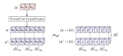
Figure S5: An example of storing the relevant data structures as contiguous pointers.

At the core of every deep learning framework such as PyTorch [55], TensorFlow [72] and Jax [73] lies a library of GPU-accelerated tensor algebra primitives. These primitives operate on contiguous arrays of known size that store relevant numerical quantities (e.g. network parameters and real-world data). Such arrays are often manipulated in a vectorised (batched) manner so that the number of explicit loops is reduced to a minimum.

The toy example of previous section suggests that implementing our optimisation procedure using tensor algebra primitives is not straightforward. For example, the size of each $\mathcal{SC}_{\mathbf{x}}$ set is dynamic and depends on the batch $\mathcal{U}$ sampled at the current iteration. In addition, finding out coupled pairs requires a search operation to determine which of $\mathbf{\underline{XY}}=\mathbf{x}\otimes\mathbf{x}^{\prime}$ corresponds to a Hamiltonian term.

In principle, one might still leverage GPU parallelism by writing a specialised CUDA code implementing the variational optimisation. However, this is beyond our ability. Instead, in the remainder of this Supplementary we discuss how to implement key components of ANQS variational optimisation using only a stringent set of tensor algebra primitives, specifically that of PyTorch software library.

In this Section we outline the main principles behind our implementation, while specific routines such as FindCoupledPairs and MatrixElement are covered in the subsequent sections. We illustrate every non-trivial operation with the arrays corresponding to the model problem considered in Section S2.

S3.1 Contiguous arrays

The first guiding principle of our implementation is storing information contiguously, as illustrated in Fig. S5A, which enables the use of vectorised PyTorch primitives. As discussed in the main text, we represent $N$-bit basis vectors as tuples of $N_{\rm\frac{int}{vec}}\coloneqq\left\lceil\frac{N}{N_{\rm\frac{bits}{int}}}\right\rceil$ integers, where $N_{\rm\frac{bits}{int}}$ is the number of bits contained in a single integer number. In our case $N=4$ and thus we assume only one integer is needed per basis vectors. As a result, the batch of three unique samples is stored as an integer array $\mathcal{U}$ of length 3, or, equivalently, of shape $[N_{\rm unq},1]$. For the sake of clarity, in our diagrams, the first and second dimensions of each tensor are depicted horizontally and vertically, respectively. This representation is opposite to the conventional notion where a tensor with shape $[N,1]$ is viewed as a column vector. If more than one integer is required to represent a basis vector, $\mathcal{U}$ becomes an array of shape $\left[N_{\rm unq},N_{\rm\frac{int}{vec}}\right]$. In this case all procedures described in this supplementary can be generalised to account for the extra array dimension (see our code for more details [69]).

In Fig. S5 we emphasise that all procedures return contiguous arrays too. For example, one can see that the FindCoupledPairs procedure takes an array $\mathcal{U}$ as input and outputs two arrays $\mathbf{x}$ and $\mathbf{x}^{\prime}$. These arrays store concatenated first and second elements in each pair of every $\mathcal{SC}_{\mathbf{x}}$ respectively.

S3.2 Pointer arithmetic

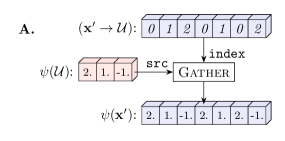
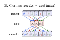
Figure S6: A. Efficient evaluation of ansatz amplitudes using Gather routine. The amplitudes are calculated only for unique basis vectors and then distributed as necessary. B. An example Gather operation.

The second key aspect of our code is the use of pointer arithmetic. Suppose one has an array A of length $L_{\texttt{A}}$. We assume that an array $\left({\texttt{B}}\rightarrow{\texttt{A}}\right)$ is an array of pointers to A if $\left({\texttt{B}}\rightarrow{\texttt{A}}\right)$ is an array of integer numbers ranging from $0$ to $L_{\texttt{A}}-1$ inclusively. In this case we interpret the $i$-th element of $\left({\texttt{B}}\rightarrow{\texttt{A}}\right)$ as a pointer to the $\left({\texttt{B}}\rightarrow{\texttt{A}}\right)[i]$-th element of A. Arrays $\left({\mathbf{x}}\rightarrow{\mathcal{U}}\right)$ and $\left({\mathbf{x}^{\prime}}\rightarrow{\mathcal{U}}\right)$ depicted in Fig. S5 are specific examples of pointer arrays. They represent arrays $\mathbf{x}$ and $\mathbf{x}^{\prime}$ by storing not $\mathbf{x}_{0},\mathbf{x}_{1},\ldots$ themselves, but their indices instead. For example, $\mathbf{x}[3]=\mathbf{x}_{1}$ and thus $\left({\mathbf{x}}\rightarrow{\mathcal{U}}\right)[3]=1$.

The pointer arithmetic is crucial for our implementation for two reasons. First, it allows one to avoid redundant computation, as illustrated in Fig. S6A. One obtains the amplitudes for each $\mathbf{x}^{\prime}$ in $\mathcal{SC}$ by reusing the known values of amplitudes for basis vectors in $\mathcal{U}$, rather than evaluating them directly. The substitution is performed with a standard tensor algebra routine Gather depicted in Fig. S6B. As input, this routine takes a src array and an array index of pointers to src. As output, it produces the result array defined as $\texttt{result}[i]=\texttt{src}[\texttt{index}[i]]$. We call this process dereferencing of index with respect to src. Note that the same pointer array might be dereferenced with respect to different source arrays. For example, $\textsc{Gather}(\texttt{src}:\psi(\mathcal{U}),\texttt{index}:\left({\mathbf{x}^{\prime}}\rightarrow{\mathcal{U}}\right))=\psi(\mathbf{x}^{\prime})$, while $\textsc{Gather}(\texttt{src}:\mathcal{U},\texttt{index}:\left({\mathbf{x}^{\prime}}\rightarrow{\mathcal{U}}\right))=\mathbf{x}^{\prime}$.

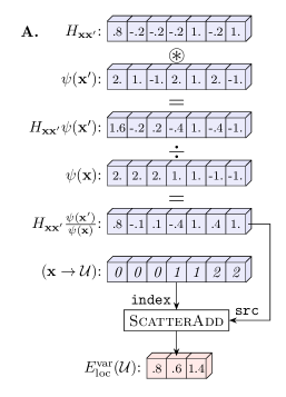
Figure S7: A. Efficient evaluation of $E_{\rm loc}^{\rm var}$ where the dynamic range summations are performed with ScatterAdd routine. B. An example ScatterAdd operation.

The second advantage of pointer arithmetic is that it enables summation over dynamically defined ranges of indices as illustrated in Fig. S7A. Suppose we employed MatrixElement function to obtain the array $H_{\mathbf{x}\mathbf{x}^{\prime}}$ of Hamiltonian matrix elements. To obtain $E_{\rm loc}^{\rm var}(\mathbf{x})$ one has to perform three following steps:

1. Multiply it elementwise by an array $\psi(\mathbf{x}^{\prime})$;

2. Divide it elementwise by an array $\psi(\mathbf{x})$;

3. Sum the values $H_{\mathbf{x}\mathbf{x}^{\prime}}\frac{\psi(\mathbf{x}^{\prime})}{\psi(\mathbf{x})}$ corresponding to the same unique $\mathbf{x}$.

The summation at the last stage can be performed with another tensor algebra routine known as ScatterAdd. This routine adds the $i$-th element of an array src to the $\texttt{index}[i]$-th element of array result and is depicted in Fig. S7B.

S3.3 Notation remarks

Let us make two remarks regarding the notation and the diagrams representing GPU operations. First, the names of arrays which store pointers of any kind will necessarily include the symbol $\rightarrow$. Second, we use different font styling to display the content of arrays of different nature: (i) we depict in bold the content of arrays storing values corresponding to $N$-bit vectors, e.g. $\mathbf{x}$ and $\mathbf{x}^{\prime}$; (ii) we display in italics the content of arrays storing pointers of any kind, e.g. $\left({\mathbf{x}}\rightarrow{\mathcal{U}}\right)$; (iii) we use normal styling for the content of arrays storing genuine floating point or integer values, e.g. $\psi(\mathbf{x})$ or $E_{\rm loc}^{\rm var}(\mathbf{x})$.

S3.4 Preparation

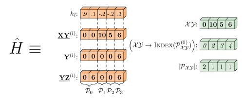
Figure S8: Storing the Hamiltonian as a set of tensors.

Before the start of each simulation we preprocess the Hamiltonian to represent it as a set of tensors stored on a GPU as depicted in Fig. S8. For example, $h_{l}$ is a contiguous array storing the weights of all Hamiltonian terms, i.e. $h_{l}[0]=h_{0}$. The arrays $\mathbf{\underline{XY}}^{(l)}$, $\mathbf{Y}^{(l)}$ and $\mathbf{\underline{YZ}}^{(l)}$ are constructed in a similar way.

We also introduce three auxiliary arrays to represent the fact that each unique $\mathbf{\underline{XY}}^{(l)}$ might correspond to several terms constituting the set $\mathcal{P}_{\mathbf{\underline{XY}}}$. In Fig. S8 we show how elements of the arrays $h_{l}$, $\mathbf{Y}^{(l)}$ and $\mathbf{\underline{YZ}}^{(l)}$ are grouped into the corresponding sets. For example, the zeroth and first elements of these arrays correspond to $\mathcal{P}_{\mathbf{\underline{XY}}_{0}}$, which we denote for brevity as $\mathcal{P}_{0}$. The first auxiliary array $\mathcal{XY}$ is an array of unique $\mathbf{\underline{XY}}$ vectors themselves. Second, $\left({\mathcal{XY}}\rightarrow{\textsc{Index}(\mathcal{P}_{\mathcal{XY}}^{(0)})}\right)$ stores pointers to the first elements in $\mathcal{P}_{\mathbf{\underline{XY}}}$ for each $\mathbf{\underline{XY}}$ in $\mathcal{XY}$. For example, $\left({\mathcal{XY}}\rightarrow{\textsc{Index}(\mathcal{P}_{\mathcal{XY}}^{(0)})}\right){}[1]=2$ since the set $\mathcal{P}_{1}$ starts from the position 2 in arrays $h_{l}$, $\mathbf{Y}^{(l)}$ and $\mathbf{\underline{YZ}}^{(l)}$. Finally, the array $\left|\mathcal{P}_{\mathbf{\underline{XY}}}\right|$ stores the number of terms in $\mathcal{P}_{\mathbf{\underline{XY}}}$ for each unique $\mathbf{\underline{XY}}$. These three arrays will prove instrumental for our implementation of MatrixElement discussed further.

S4 GPU implementation: main functions

In this section we cover two key procedures of ANQS optimisation: LoopOverBatch and MatrixElement. The implementation of LoopOverTerms is similar to that of LoopOverBatch and can be found in our code [69]. The discussion on implementation of LoopOverTrie is left for Section S5.

S4.1 LoopOverBatch implementation

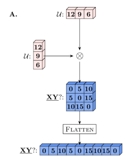
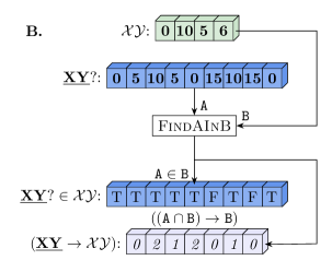
Figure S9: Two first stages of LoopOverBatch A. One evaluates candidate $\mathbf{\underline{XY}}$ bit vectors in a vectorised manner. B. One invokes custom a FindAInB function to obtain a boolean mask indicating whether a candidate $\mathbf{\underline{XY}}$ belongs to $\mathcal{XY}$. As well, one obtains an array of pointers from “successful” candidate $\mathbf{\underline{XY}}$ to $\mathcal{XY}$.

We split GPU implementation of LoopOverBatch algorithm into three main stages.

Stage 1: Find candidate $\mathbf{\underline{XY}}$

The first stage is illustrated in Fig. S9A. It in a vectorised way all possible candidate vectors $\mathbf{\underline{XY}}=\mathbf{x}\otimes\mathbf{x}^{\prime},\ \forall\mathbf{x},\mathbf{x}^{\prime}\in\mathcal{U}$; we denote an array of such candidates as $\mathbf{\underline{XY}}?$. To that end, one applies the bitwise XOR operation to two copies of $\mathcal{U}$, with one reshaped into a column vector. The broadcasting rules of PyTorch ensure that the resulting 2D array $\mathbf{\underline{XY}}?$ is a matrix of size $N_{\rm unq}\times N_{\rm unq}$. At the end of this stage one flattens $\mathbf{\underline{XY}}?$ into a 1D array by concatenating its rows.

Stage 2: Filter candidate $\mathbf{\underline{XY}}$

The second stage is shown in Fig. S9B. It invokes a custom function FindAInB to find which of the candidate $\mathbf{\underline{XY}}{}?$ correspond to bit vectors in $\mathcal{XY}$.

To explain FindAInB functioning, suppose we feed it two integer arrays, A and B. We presume that there are no repeated values in the array B, while there might be some in A. FindAInB produces two output arrays. The first output array $\texttt{A}\in\texttt{B}$ is a boolean mask indicating whether the elements of A can be found in B. In our example $(\texttt{A}\in\texttt{B})[1]=\textsc{True}$ since $\mathbf{\underline{XY}}?[1]=\mathbf{5}$ belongs to $\mathcal{XY}$. At the same time $(\texttt{A}\in\texttt{B})[5]=\textsc{False}$ since $\mathbf{\underline{XY}}?[5]=\mathbf{15}$ does not belong to $\mathcal{XY}$

The second output array $\left({(\texttt{A}\cap\texttt{B})}\rightarrow{\texttt{B}}\right)$ contains the pointers from those elements of A which belong to B (i.e. $\texttt{A}\cap\texttt{B}$) to their corresponding positions in B. Its length is equal to the number of elements in A which belong to B and the order between elements is the same as in the initial array A. For example, $(\left({(\texttt{A}\cap\texttt{B})}\rightarrow{\texttt{B}}\right))[1]=\it{2}$ because the second element in $\mathbf{\underline{XY}}?$ corresponds to the third element in $\mathcal{XY}$.

In what follows we refer to the array $\texttt{A}\in\texttt{B}$ as $\mathbf{\underline{XY}}?\in\mathcal{XY}$, and to the array $\left({(\texttt{A}\cap\texttt{B})}\rightarrow{\texttt{B}}\right)$ as $\left({\mathbf{\underline{XY}}}\rightarrow{\mathcal{XY}}\right)$. Since $\left({\mathbf{\underline{XY}}}\rightarrow{\mathcal{XY}}\right)$ corresponds to all correctly coupled $\mathbf{x}$ and $\mathbf{x}^{\prime}$, its length is equal to the length of $\left({\mathbf{x}}\rightarrow{\mathcal{U}}\right)$ and $\left({\mathbf{x}^{\prime}}\rightarrow{\mathcal{U}}\right)$ representing $\mathcal{SC}$.

Stage 3: Obtain $\mathcal{SC}$

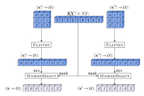
Figure S10: The last stage of LoopOverBatch. One obtains $\mathcal{SC}$ by masking off the pointers to uncoupled pairs of $\mathbf{x}$ and $\mathbf{x}^{\prime}$.

The third stage is depicted in Fig. S10. During this stage one uses the boolean mask $\mathbf{\underline{XY}}?\in\mathcal{XY}$ to obtain $\left({\mathbf{x}}\rightarrow{\mathcal{U}}\right)$ and $\left({\mathbf{x}^{\prime}}\rightarrow{\mathcal{U}}\right)$. To that end, one forms a 2D array of candidate pointers from $\mathbf{x}$ to $\mathcal{U}$ which we denote as $\left({\mathbf{x}?}\rightarrow{\mathcal{U}}\right)$. The first row of this array contains only zeros since it corresponds to all $\mathbf{\underline{XY}}{}?$ formed with $\mathbf{x}_{0}$ being the first element in the pair. Correspondingly, the second row contains only ones, the third contains only twos and so on. The 2D array $\left({\mathbf{x}^{\prime}?}\rightarrow{\mathcal{U}}\right)$ is constructed in a similar way, except for its columns consisting of the same values. One flattens $\left({\mathbf{x}?}\rightarrow{\mathcal{U}}\right)$ and $\left({\mathbf{x}^{\prime}?}\rightarrow{\mathcal{U}}\right)$ and applies the boolean mask $\mathbf{\underline{XY}}?\in\mathcal{XY}$ to filter out only those pointers which correspond to the actually coupled pairs $(\mathbf{x},\mathbf{x}^{\prime})$.

S4.2 MatrixElement implementation

The GPU implementation of MatrixElement consists of three consecutive stages.

Stage 1: Expand the pointers

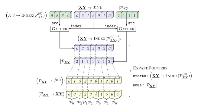
Figure S11: The first stage of MatrixElement. For each coupling $\mathbf{\underline{XY}}$ one substitutes its pointer to $\mathcal{XY}$ with a contiguous sequence of pointers $\hat{P}^{(l)}$ in $\mathcal{P}_{\mathbf{\underline{XY}}}$. To that end, one employs a custom ExpandPointers function described fin Section S6.

The first stage is illustrated in Fig. S11. Since each $\mathbf{\underline{XY}}$ might correspond to several terms in Hamiltonian, this stage substitutes every pointer in $\left({\mathbf{\underline{XY}}}\rightarrow{\mathcal{XY}}\right)$ with a sequence of pointers to $\mathbf{\underline{YZ}}$ corresponding to the given $\mathbf{\underline{XY}}$. Let us provide an example. The first element of $\left({\mathbf{\underline{XY}}}\rightarrow{\mathcal{XY}}\right)$ is $\it 0$ and thus it points to the first element of $\mathcal{XY}$. This element $\mathcal{XY}{}[0]$ corresponds to $\mathbf{\underline{XY}}=\bf 0$ which is represented with Hamiltonian terms $\hat{P}_{0}$ and $\hat{P}_{1}$. Thus, $(\left({\mathbf{\underline{XY}}}\rightarrow{\mathcal{XY}}\right))[0]$ should be expanded to pointers $\it 0$ and $\it 1$. We store these pointers contiguously in a larger array $\left({\mathcal{P}_{\mathbf{\underline{XY}}}}\rightarrow{\hat{P}^{(l)}}\right)$. In addition, we keep the reverse pointers from each element in $\mathcal{P}_{\mathbf{\underline{XY}}}$ to its parent $\mathbf{\underline{XY}}$ in an array $\left({\mathcal{P}_{\mathbf{\underline{XY}}}}\rightarrow{\mathbf{\underline{XY}}}\right)$ of the same size as $\left({\mathcal{P}_{\mathbf{\underline{XY}}}}\rightarrow{\hat{P}^{(l)}}\right)$.

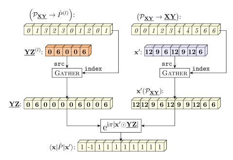
Figure S12: The second stage of MatrixElement. One employs the pointers to $\hat{P}^{(l)}$ to evaluate the matrix elements $\braket{\mathbf{x}}{\hat{P}}{\mathbf{x}^{\prime}}$ for all $\hat{P}$ coupling each pair $(\mathbf{x},\mathbf{x}^{\prime})$.

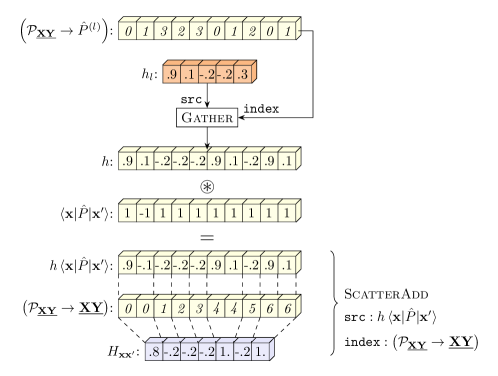
Figure S13: The third stage of MatrixElement. One employs ScatterAdd function to sum all $h\braket{\mathbf{x}}{\hat{P}}{\mathbf{x}^{\prime}}$ corresponding to each pair $(\mathbf{x},\mathbf{x}^{\prime})$ into $H_{\mathbf{x}\mathbf{x}^{\prime}}$.

In more details this stage proceeds as follows.

1. First, one uses the Gather operation to obtain arrays $\left({\mathbf{\underline{XY}}}\rightarrow{\textsc{Index}(\mathcal{P}_{\mathbf{\underline{XY}}}^{(0)})}\right)$ and $\left|\mathcal{P}_{\mathbf{\underline{XY}}}\right|$ by dereferencing the pointers $\left({\mathbf{\underline{XY}}}\rightarrow{\mathcal{XY}}\right)$ with respect to the arrays $\left({\mathcal{XY}}\rightarrow{\textsc{Index}(\mathcal{P}_{\mathcal{XY}}^{(0)})}\right)$ and $\left|\mathcal{P}_{\mathcal{XY}}\right|$. Thus, each element of $\left({\mathbf{\underline{XY}}}\rightarrow{\textsc{Index}(\mathcal{P}_{\mathbf{\underline{XY}}}^{(0)})}\right)$ stores a pointer to the first Hamiltonian term in the set $\mathcal{P}_{\mathbf{\underline{XY}}}$. Similarly, the array $\left|\mathcal{P}_{\mathbf{\underline{XY}}}\right|$ stores the sizes of the corresponding $\mathcal{P}_{\mathbf{\underline{XY}}}$ sets.

2. As a second step, one expands pointers to the first $\mathcal{P}_{\mathbf{\underline{XY}}}$ elements (which we further refer to as starts) and the sizes of $\mathcal{P}_{\mathbf{\underline{XY}}}$ into a contiguous array containing pointers to all elements in $\mathcal{P}_{\mathbf{\underline{XY}}}$. This is achieved with a custom function ExpandPointers, which is explained in more details in Section S6. The resulting pointers are stored in the array $\left({\mathcal{P}_{\mathbf{\underline{XY}}}}\rightarrow{\hat{P}^{(l)}}\right)$

3. Finally, one obtains the reverse pointers $\left({\mathcal{P}_{\mathbf{\underline{XY}}}}\rightarrow{\mathbf{\underline{XY}}}\right)$ by repeating the index of each $\mathbf{\underline{XY}}$ element $\left|\mathcal{P}_{\mathbf{\underline{XY}}}\right|$ times as illustrated in the last line of Fig. S11. This can be easily achieved with the standard RepeatInterleave routine of the PyTorch software library.

Stage 2: Calculate term expectation values

The second stage of MatrixElement calculation is shown in Fig. S12. First, one dereferences the pointers $\left({\mathcal{P}_{\mathbf{\underline{XY}}}}\rightarrow{\hat{P}^{(l)}}\right)$ with respect to the array $\mathbf{\underline{YZ}}^{(l)}$ to obtain an array of $\mathbf{\underline{YZ}}$ corresponding to each element in $\mathcal{P}_{\mathbf{\underline{XY}}}$. Second, one dereferences the pointers $\left({\mathcal{P}_{\mathbf{\underline{XY}}}}\rightarrow{\mathbf{\underline{XY}}}\right)$ with respect to the array $\mathbf{x}^{\prime}$. Thus, one obtains an array $\mathbf{x}^{\prime}(\mathcal{P}_{\mathbf{\underline{XY}}})$ which contains all $\mathbf{x}^{\prime}$ required to evaluate $\braket{\mathbf{x}}{\hat{P}}{\mathbf{x}^{\prime}}$. Finally, one feeds both $\mathbf{\underline{YZ}}$ and $\mathbf{x}^{\prime}(\mathcal{P}_{\mathbf{\underline{XY}}})$ into a simple arithmetic function calculating $\mathrm{e}^{\mathrm{i}\pi\left|\mathbf{x}^{\prime}\odot\mathbf{\underline{YZ}}\right|}$ elementwise. As a result, one obtains the array containing the values of $\braket{\mathbf{x}}{\hat{P}}{\mathbf{x}^{\prime}}$.

Stage 3: Scatter term expectation values

The third stage is depicted in Fig. S13. First, one dereferences the pointers $\left({\mathcal{P}_{\mathbf{\underline{XY}}}}\rightarrow{\hat{P}^{(l)}}\right)$ with respect to the array $h_{l}$. Thus, one fetches the weights of Hamiltonian terms for corresponding $\braket{\mathbf{x}}{\hat{P}}{\mathbf{x}^{\prime}}$. Second, one multiplies $h$ and $\braket{\mathbf{x}}{\hat{P}}{\mathbf{x}^{\prime}}$ elementwise to obtain an array $h_{l}\braket{\mathbf{x}}{\hat{P}}{\mathbf{x}^{\prime}}$. Finally, one employs the ScatterAdd routine to sum the values of $h_{l}\braket{\mathbf{x}}{\hat{P}}{\mathbf{x}^{\prime}}$ corresponding to the same $\mathbf{\underline{XY}}$. During ScatterAdd the array $\left({\mathcal{P}_{\mathbf{\underline{XY}}}}\rightarrow{\mathbf{\underline{XY}}}\right)$ serves as the index input argument.

S5 GPU implementation: prefix tree operations

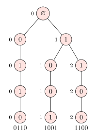
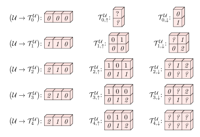
Figure S14: The prefix tree data structures for the batch of unique samples $\mathcal{U}$.

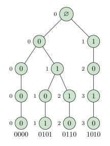
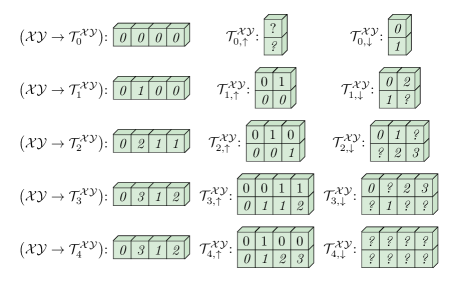
Figure S15: The prefix tree data structures for the set $\mathcal{XY}$ of unique $\mathbf{\underline{XY}}$ strings representing Hamiltonian terms.

S5.1 Prefix tree data structures

In our GPU implementation we store the prefix tree nodes as contiguous arrays, as opposed to storing them as individual data structures introduced in the main text. As an example, let us consider the batch of unique samples $\mathcal{U}$ and its prefix tree $\mathcal{T}^{\mathcal{U}}$. For the $i$-th level of the prefix tree we store three arrays denoted as $\left({\mathcal{U}}\rightarrow{\mathcal{T}^{\mathcal{U}}_{i}}\right)$, $\mathcal{T}^{\mathcal{U}}_{i,\uparrow}$ and $\mathcal{T}^{\mathcal{U}}_{i,\downarrow}$ as depicted in Fig. S14.

1. The array $\left({\mathcal{U}}\rightarrow{\mathcal{T}^{\mathcal{U}}_{i}}\right)$ has a shape $[N_{\rm unq}{},1]$. Its $k$-th element points to a node at the $i$-th level of the prefix tree that corresponds to the $k$-th basis vector in $\mathcal{U}$. For example, at the level 2 of the prefix tree $\left({\mathcal{U}}\rightarrow{\mathcal{T}^{\mathcal{U}}_{2}}\right)[0]=\it{2}$ since the first two symbols of $\mathbf{x}_{0}$ are $11$, and this prefix path leads to the node 2 of level 2. At the same time, $\left({\mathcal{U}}\rightarrow{\mathcal{T}^{\mathcal{U}}_{0}}\right)[k]=0\ \forall k$ since all vectors in $\mathcal{U}$ start from an empty string $\varnothing$.

2. The array $\mathcal{T}^{\mathcal{U}}_{i,\uparrow}$ has a shape $\left[\ \left|\mathcal{T}^{\mathcal{U}}_{i}\right|,2\right]$, where $\left|\mathcal{T}^{\mathcal{U}}_{i}\right|$ is the number of nodes at the $i$-th prefix tree level. It stores in a contiguous way the fields value and parent of the Node data structure introduced in the main text. Specifically, $\mathcal{T}^{\mathcal{U}}_{i,\uparrow}[l,0]$ stores $x_{i}$, while $\mathcal{T}^{\mathcal{U}}_{i,\uparrow}[l,1]$ keeps the pointer to the parent node at the previous level. For example, the bit value of node 2 at level 2 is equal to 1, and thus $\mathcal{T}^{\mathcal{U}}_{2,\uparrow}[2,0]=1$. At the same time, its parent is node 1 at level 1, and thus $\mathcal{T}^{\mathcal{U}}_{2,\uparrow}[2,1]=\it 1$. Let us note that $\mathcal{T}^{\mathcal{U}}_{0,\uparrow}$ always has a shape $[1,2]$ and we fill it with NaNs, since this node does not have a definite value and does not have a parent node.

3. The array $\mathcal{T}^{\mathcal{U}}_{i,\downarrow}$ has a shape $\left[\ \left|\mathcal{T}^{\mathcal{U}}_{i}\right|,2\right]$ too. It stores in a contiguous way the children field of the Node data structure. In particular, $\mathcal{T}^{\mathcal{U}}_{i,\downarrow}[l,0]$ stores the pointer to a child with the value of 0 of the node $l$. Similarly, $\mathcal{T}^{\mathcal{U}}_{i,\downarrow}[l,1]$ stores the pointer to a child with the value 1. In our diagrams these children nodes are to the left and to the right of the parent node correspondingly. If a node does not have a child, we store NaN instead of a pointer. For example, the node 0 at level 2 does not have a child with the value 0, and thus $\mathcal{T}^{\mathcal{U}}_{i,\downarrow}[2,0]=\it{?}$. At the same time, the same node does have a child with the bit value 1, which is a node 0 at level 3. Thus, $\mathcal{T}^{\mathcal{U}}_{i,\downarrow}[2,0]=\it{0}$. At the last prefix tree level nodes do not have children and thus $\mathcal{T}^{\mathcal{U}}_{N,\downarrow}$ is a redundant array filled with NaNs.

For the sake of completeness, in Fig. S15 we provide the prefix tree data structures for the set $\mathcal{XY}$.

S5.2 ConstructPrefixTree implementation

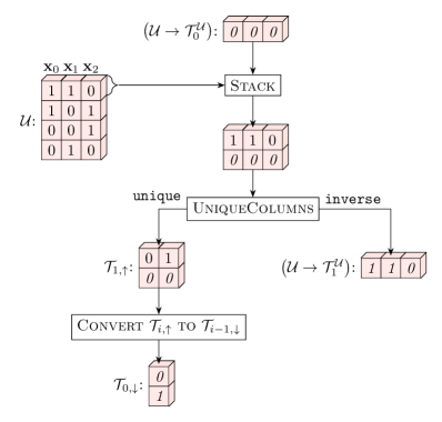
Figure S16: An iteration of the ConstructPrefixTree algorithm.

The idea of ConstructPrefixTree is to obtain the relevant prefix tree structures level by level starting from $\left({\mathcal{U}}\rightarrow{\mathcal{T}^{\mathcal{U}}_{0}}\right)$ and $\mathcal{T}^{\mathcal{U}}_{0,\uparrow}$. We illustrate how the arrays of level 1 can be obtained from the arrays of level 0 in Fig. S16. More generally, the same procedure is applicable to obtain the arrays of level $i$ from the arrays of level $i-1$.

1. First, one stacks the array containing $i$-th bits of all vectors in $\mathcal{U}$ on top of the array $\left({\mathcal{U}}\rightarrow{\mathcal{T}^{\mathcal{U}}_{i-1}}\right)$ to form an array of shape $[N_{\rm unq},2]$. This array essentially contains all non-unique prefixes at $i$-th level: the first row stores node values, while the second row contains pointers to the parents.

2. Two non-unique prefixes that have the same bit value and a parent are considered identical and should be merged into a single prefix. Thus, one feeds non-unique prefixes into a UniqueColumns function which produces two output arrays. The first output is a 2D array of shape $\left[\ \left|\mathcal{T}^{\mathcal{U}}_{i}\right|,2\right]$ containing only unique prefixes; by inspection it can be seen that this array is equivalent $\mathcal{T}^{\mathcal{U}}_{i,\uparrow}$. The second output is an array containing pointers from non-unique prefixes to the unique ones. Since each non-unique prefix is associated with a basis vector in $\mathcal{U}$, this array represents $\left({\mathcal{U}}\rightarrow{\mathcal{T}^{\mathcal{U}}_{i}}\right)$. The UniqueColumns is our custom lower-level function and we cover it in Section S6.

3. Finally, one uses the obtained arrays to fill the array $\mathcal{T}^{\mathcal{U}}_{i-1,\downarrow}$ at the previous level. First, one creates an array filled with NaNs of the same shape as $\mathcal{T}^{\mathcal{U}}_{i-1,\uparrow}$. Then, one scatters into it the values from array $\mathcal{T}^{\mathcal{U}}_{i,\downarrow}$ according to the following rule:

   $$\mathcal{T}^{\mathcal{U}}_{i-1,\downarrow}[\mathcal{T}^{\mathcal{U}}_{i,\uparrow}[l,1],\mathcal{T}^{\mathcal{U}}_{i,\uparrow}[l,0]]=l\ \forall l\in 1..\left|\mathcal{T}^{\mathcal{U}}_{i}\right|.$$ (19)

   In other words, for each node in $\mathcal{T}^{\mathcal{U}}_{i}$ we find its parent node $\mathcal{T}^{\mathcal{U}}_{i,\uparrow}[l,1]$ and indicate that this node has a child $\it l$ having the bit value $\mathcal{T}^{\mathcal{U}}_{i,\uparrow}[l,0]$

S5.3 LoopOverTrie implementation

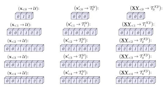
Figure S17: Arrays obtained during one full run of LoopOverTrie.

The LoopOverTrie algorithm described in Methods builds coupled pairs $(\mathbf{x},\mathbf{x}^{\prime})$ bit by bit. For a given $\mathbf{x}$ and prefix tree level $i$ it calculates all acceptable prefixes $\mathbf{x}^{\prime}_{<i}$ and the corresponding coupling $\mathbf{\underline{XY}}_{<i}$. The idea of our GPU implementation is to store the pointers to valid $\mathbf{x}^{\prime}_{<i}$ and $\mathbf{\underline{XY}}_{<i}$ in an array for each $\mathbf{x}$ and update them level by level. In addition, we concatenate all such pointer arrays to vectorise the algorithm across all $\mathbf{x}$ in $\mathcal{U}$.

Specifically, for each prefix tree level we obtain three arrays shown in Fig. S17:

1. The array $\left({\mathbf{x}_{<i}}\rightarrow{\mathcal{U}}\right)$ serves the vectorisation purpose and indicates chunks of other arrays which correspond to different $\mathbf{x}$ being input to ConstructPrefixTree. For example, at the level 0 we start with empty prefixes $\varnothing$ corresponding to every vector in $\mathcal{U}$ and thus $\left({\mathbf{x}_{<0}}\rightarrow{\mathcal{U}}\right)=[\it 0,\it 1,\it 2]$.

2. The array $\left({\mathbf{x}^{\prime}_{<i}}\rightarrow{\mathcal{T}^{\mathcal{U}}_{i}}\right)$ stores pointers to valid $\mathbf{x}^{\prime}_{<i}$ prefixes for every $\mathbf{x}$ in $\mathcal{U}$. For example, at level 0 any vector in $\mathcal{U}$ can be coupled only to a single prefix $\varnothing$ and thus $\left({\mathbf{x}^{\prime}_{<0}}\rightarrow{\mathcal{T}^{\mathcal{U}}_{0}}\right)=[\it 0,\it 0,\it 0]$.

3. The array $\left({\mathbf{\underline{XY}}_{<i}}\rightarrow{\mathcal{T}^{\mathcal{XY}}_{i}}\right)$ stores pointers to valid $\mathbf{\underline{XY}}_{<i}$ prefixes in a way similar to $\left({\mathbf{x}^{\prime}_{<i}}\rightarrow{\mathcal{T}^{\mathcal{U}}_{i}}\right)$.

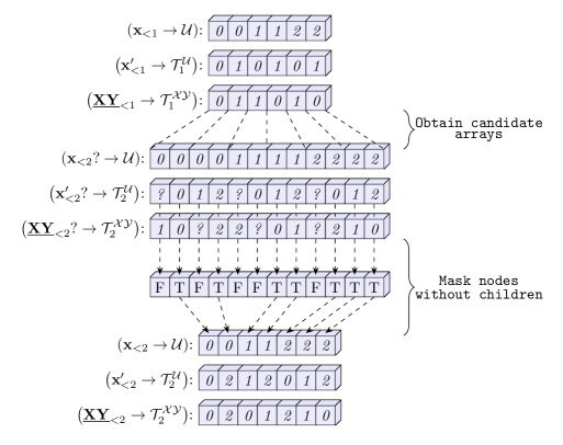
Figure S18: An iteration of LoopOverTrie GPU implementation.

A single iteration of the algorithm which produces level 2 arrays given the arrays at level 1 is shown in Fig. S18. More generally, obtaining arrays for level $i$ from the arrays of level $i-1$ involves the following steps.

1. First, we substitute every pointer to a valid prefix $\mathbf{x}^{\prime}_{<i-1}$ ($\mathbf{\underline{XY}}_{<i-1}$) with the pointers to its possible children (including NaNs for non-existing children). This produces the arrays of candidate pointers $\left({\mathbf{x}^{\prime}_{<i}?}\rightarrow{\mathcal{T}^{\mathcal{U}}_{i}}\right)$ and $\left({\mathbf{\underline{XY}}_{<i}?}\rightarrow{\mathcal{T}^{\mathcal{XY}}_{i}}\right)$ twice the length of the initial arrays. Specifically, entries of the array $\left({\mathbf{x}^{\prime}_{<i}?}\rightarrow{\mathcal{T}^{\mathcal{U}}_{i}}\right)$ are as follows:

   $$\begin{gathered}\left({\mathbf{x}^{\prime}_{<i}}\rightarrow{\mathcal{T}^{\mathcal{U}}_{i}}\right)[2k]=\mathcal{T}^{\mathcal{U}}_{i-1,\downarrow}[k,0];\\ \left({\mathbf{x}^{\prime}_{<i}}\rightarrow{\mathcal{T}^{\mathcal{U}}_{i}}\right)[2k+1]=\mathcal{T}^{\mathcal{U}}_{i-1,\downarrow}[k,1];\end{gathered}$$ (20)

   In other words, the $k$-th valid prefix pointer in the array $\left({\mathbf{x}^{\prime}_{<i-1}}\rightarrow{\mathcal{T}^{\mathcal{U}}_{i-1}}\right)$ is substituted with the pointers to its left and right children at the positions $2k$ and $2k+1$ respectively. The array $\left({\mathbf{\underline{XY}}_{<i}?}\rightarrow{\mathcal{T}^{\mathcal{XY}}_{i}}\right)$ is obtained in a similar way, however, with a subtlety: for a given $\mathbf{\underline{XY}}_{<i-1}$ the order of its children in the array $\left({\mathbf{\underline{XY}}_{<i}?}\rightarrow{\mathcal{T}^{\mathcal{XY}}_{i}}\right)$ depends on the $i$-th bits of both $\mathbf{x}{}$ and $\mathbf{x}^{\prime}{}$. For example, $\left({\mathbf{x}^{\prime}_{<i}}\rightarrow{\mathcal{T}^{\mathcal{U}}_{i}}\right)[2k]$ corresponds to moving to the left child of $\mathbf{x}^{\prime}_{<i-1}$, i.e. appending 0 to it. However, if $x_{i}=1$, then $XY_{i}=x_{i}\otimes 0=1$, and thus $\left({\mathbf{\underline{XY}}_{<i}?}\rightarrow{\mathcal{T}^{\mathcal{XY}}_{i}}\right)[2k]$ should contain the pointer to the right child of $\left({\mathbf{\underline{XY}}_{<i-1}}\rightarrow{\mathcal{T}^{\mathcal{XY}}_{i-1}}\right)[k]$. This is expressed with the following equations:

   $$\begin{gathered}\left({\mathbf{\underline{XY}}_{<i}}\rightarrow{\mathcal{T}^{\mathcal{XY}}_{i}}\right)[2k]=\mathcal{T}^{\mathcal{XY}}_{i-1,\downarrow}[k,0\otimes\mathbf{x}_{k}[i]];\\ \left({\mathbf{\underline{XY}}_{<i}}\rightarrow{\mathcal{T}^{\mathcal{XY}}_{i}}\right)[2k+1]=\mathcal{T}^{\mathcal{XY}}_{i-1,\downarrow}[k,1\otimes\mathbf{x}_{k}[i]];\end{gathered}$$ (21)

   Finally, to keep track of the vectorised $\mathbf{x}$, we double each element in $\left({\mathbf{x}_{<i-1}}\rightarrow{\mathcal{U}}\right)$:

   $$\left({\mathbf{x}_{<i}}\rightarrow{\mathcal{U}}\right)[2k]=\left({\mathbf{x}_{<i}}\rightarrow{\mathcal{U}}\right)[2k+1]=\left({\mathbf{x}_{<i-1}}\rightarrow{\mathcal{U}}\right)[k]$$ (22)

   The new arrays can be obtained using a combination of Tile, Gather and Reshape PyTorch primitives and we refer the reader to our code for more details [69].

2. Once the arrays are produced, we calculate a boolean mask which is equal to True only if child pointers are not NaN for both $\left({\mathbf{x}^{\prime}_{<i}}\rightarrow{\mathcal{T}^{\mathcal{U}}_{i}}\right)$ and $\left({\mathbf{\underline{XY}}_{<i}}\rightarrow{\mathcal{T}^{\mathcal{XY}}_{i}}\right)$.

3. Finally, we use this boolean mask to obtain arrays of valid prefixes for the current level $i$.

The array $\left({\mathbf{x}_{<N}}\rightarrow{\mathcal{U}}\right)$ obtained at the last level of LoopOverTrie is clearly equivalent to the array $\left({\mathbf{x}^{\prime}}\rightarrow{\mathcal{U}}\right)$ produced by FindCoupledPairs procedure. The arrays $\left({\mathbf{x}^{\prime}}\rightarrow{\mathcal{U}}\right)$ and $\left({\mathbf{\underline{XY}}}\rightarrow{\mathcal{XY}}\right)$ can be obtained from $\left({\mathbf{x}^{\prime}_{<N}}\rightarrow{\mathcal{T}^{\mathcal{U}}_{N}}\right)$ and $\left({\mathbf{\underline{XY}}_{<N}}\rightarrow{\mathcal{T}^{\mathcal{XY}}_{N}}\right)$ by using the correspondence between the indices of the nodes at the last level of a prefix tree, and their indices in the initial bit vector set. As described above, this correspondence is expressed with the arrays $\left({\mathcal{U}}\rightarrow{\mathcal{T}^{\mathcal{U}}_{N}}\right)$ and $\left({\mathcal{XY}}\rightarrow{\mathcal{T}^{\mathcal{XY}}_{N}}\right)$ obtained during ConstructPrefixTree.

S6 GPU implementation: auxiliary functions

S6.1 FindAInB implementation

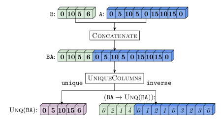
Figure S19: The first stage of FindAInB. One concatenates arrays A and B to find unique elements in their union. As well, one obtains the positions of those unique elements in the initial arrays.

As mentioned in Section S4.1 FindAInB is a function which takes two arrays A and B as input and produces two arrays $\texttt{A}\in\texttt{B}$ and $\left({(\texttt{A}\cap\texttt{B})}\rightarrow{\texttt{B}}\right)$ as output. Crucially, the array B should not contain any repeated values. We split its implementation into three stages.

Stage 1: Find unique elements in A and B union

We concatenate the arrays A and B into a single array and apply our custom function UniqueColumns to the concatenated array. We use UniqueColumns instead of default PyTorch Unique function because, in general, when several integers are used per $\mathbf{x}$, the arrays A and B will be two-dimensional, with integer values for each $\mathbf{x}$ stored in columns. Since the default PyTorch Unique function works only with 1D arrays, we have to employ our custom UniqueColumns function explained further in this section.

As depicted in Fig. S19, UniqueColumns returns two arrays. The first array $\textsc{Unq}(\texttt{B}\texttt{A})$ contains unique elements found in the union of A and B arrays. The second array $\left({\texttt{B}\texttt{A}}\rightarrow{\textsc{Unq}(\texttt{B}\texttt{A})}\right)$ can be considered as a concatenation of two arrays $\left({\texttt{B}}\rightarrow{\textsc{Unq}(\texttt{B}\texttt{A})}\right)$ and $\left({\texttt{A}}\rightarrow{\textsc{Unq}(\texttt{B}\texttt{A})}\right)$, each containing pointers from elements in B and A to the found unique values $\textsc{Unq}(\texttt{B}\texttt{A})$.

Stage 2: Finding the reverse pointers to B

The purpose of this stage is to find the reverse pointers from $\textsc{Unq}(\texttt{B}\texttt{A})$ to B. To that end, we create an array $\left({\textsc{Unq}(\texttt{B}\texttt{A})}\rightarrow{\texttt{B}}\right)$ of the same shape as $\textsc{Unq}(\texttt{B}\texttt{A})$ filled with NaNs. Then, we Scatter into this array indices of elements in B. For example, the second element in the $\left({\texttt{B}}\rightarrow{\textsc{Unq}(\texttt{B}\texttt{A})}\right)$ array is 2, which means that $\texttt{B}[1]$ is the third element of $\textsc{Unq}(\texttt{B}\texttt{A})$. Thus, we scatter 2 to the third position in the array $\left({\textsc{Unq}(\texttt{B}\texttt{A})}\rightarrow{\texttt{B}}\right)$ as depicted in Fig. S20. If, after this operation, some values are still equal to NaN, it means that there are values in $\textsc{Unq}(\texttt{B}\texttt{A})$ that can be found in A but not in B. Hence, one can apply a standard IsANumber function to $\left({\textsc{Unq}(\texttt{B}\texttt{A})}\rightarrow{\texttt{B}}\right)$ and obtain a boolean mask indicating which elements of $\textsc{Unq}(\texttt{B}\texttt{A})$ belong to B.

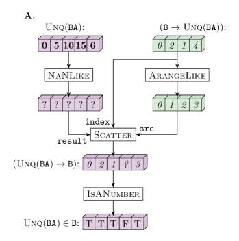
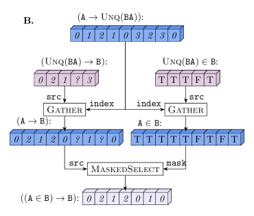
Figure S20: The two last stages of FindAInB. A. Having the pointers from B to $\textsc{Unq}(\texttt{B}\texttt{A})$, one employs Scatter to find the reverse pointers from $\textsc{Unq}(\texttt{B}\texttt{A})$ to B. As well, one obtains a boolean mask indicating whether an element in $\textsc{Unq}(\texttt{B}\texttt{A})$ can be found in B. B. One uses Gather to fetch the pointers from $\textsc{Unq}(\texttt{B}\texttt{A})$ to B for every element in A and thus obtains the pointers $\left({\texttt{A}}\rightarrow{\texttt{B}}\right)$. In addition, one obtains a boolean mask indicating whether an element in A can be found in B.

Stage 3: Finding pointers from A to B

At the final stage we Gather pointers $\left({\textsc{Unq}(\texttt{B}\texttt{A})}\rightarrow{\texttt{B}}\right)$ using the array $\left({\texttt{A}}\rightarrow{\textsc{Unq}(\texttt{B}\texttt{A})}\right)$ as index. As shown in Fig. S20B, we thus obtain an array $\left({\texttt{A}}\rightarrow{\texttt{B}}\right)$ with pointers from A to B (if some element in $\left({\texttt{A}}\rightarrow{\textsc{Unq}(\texttt{B}\texttt{A})}\right)$ is NaN, it means that the corresponding element in A does not belong to B). In a similar way, we can Gather boolean mask ${\textsc{Unq}(\texttt{B}\texttt{A})}\in{\texttt{B}}$ and obtain ${\texttt{A}}\in{\texttt{B}}$. Finally, we apply the boolean mask ${\texttt{A}}\in{\texttt{B}}$ to $\left({\texttt{A}}\rightarrow{\texttt{B}}\right)$ to keep only the valid pointers to B, as required by the use of FindAInB in FindCoupledPairs.

Computational complexity

The dominating cost of FindAInB is finding unique columns with UniqueColumns. As discussed further in Section LABEL:sec:unique_func_implementation it of complexity $\mathcal{O}\left(\left(\left|\texttt{A}\right|+\left|\texttt{B}\right|\right)\log\left(\left|\texttt{A}\right|+\left|\texttt{B}\right|\right)\right)$, which matches the figures given in Methods.

S6.2 ExpandPointers implementation

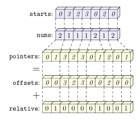
Figure S21: An example of the ExpandPointers routine. A $\texttt{starts}[i]$ pointer is substituted with a set of $\texttt{nums}[i]$ consecutive (i.e $\texttt{starts}[i],\texttt{starts}[i]+1,\ldots,\texttt{starts}[i]+\texttt{nums}[i]-1$). For the sake of simplicity, the final array of pointers is represented as a sum of two arrays offsets and saw.

The ExpandPointers procedure serves the following purpose. Suppose one has an array memory whose elements are grouped into contiguous chunks of various length. This is akin to such Hamiltonian data arrays as $h_{l}$, $\mathbf{Y}^{(l)}$ and $\mathbf{\underline{YZ}}^{(l)}$ which can be grouped according to their $\mathbf{\underline{XY}}$. ExpandPointers is a function which allows one to retrieve those contiguous chunks of memory by specifying their starting positions starts and their lengths nums. As output ExpandPointers produces an array pointers which replaces each starting pointer $\texttt{starts}[i]$ with a sequence of $\texttt{nums}[i]$ consecutive pointers to each element in the corresponding contiguous chunk. An example of the ExpandPointers action is given in Fig. S21. We split its implementation into the following steps:

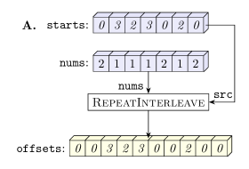
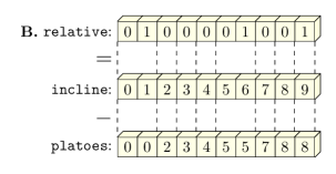
Figure S22: A. Calculation of starts array. B. Decomposition of saw array into a sum of incline and platoes arrays.

1. We represent pointers as a sum of two arrays: offsets and relative. For each expanded pointer in pointers, the offsets array contains the starting position of the chunk to which the expanded pointer belongs to. As illustrated in Fig. S22A it is trivially obtained with the standard PyTorch routine RepeatInterleave: each element of $\texttt{starts}[i]$ array is repeated $\texttt{nums}[i]$ times. The relative array contains the relative position of each extended pointer with respect to the chunk start. Obtaining relative is slightly more involved and is performed in the next steps.

2. To calculate relative we represent it as a difference of two arrays: incline and platoes. The incline array is an arithmetic progression of integers with the step 1 starting from 0. This progression represents the fact that the neighbouring expanded pointers belonging to the same chunk should differ by one. This array can be easily obtained using the standard Cumsum PyTorch function as shown in Fig. S23A.

3. However, incline does not account for the fact that this progression breaks down at the chunk borders, where increments should start from scratch. The array platoes corrects for it by counting the number of increments that are accumulated by the start of each chunk and belong to the previous chunks. The calculation of platoes is shown in Fig. S23B.

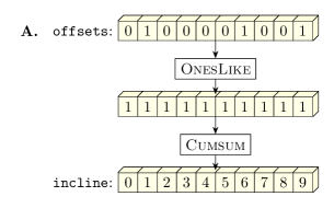
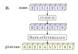
Figure S23: A. Calculation of the incline array. B. Calculation of the platoes array.

S6.3 UniqueColumns implementation

As discussed, both ConstructPrefixTree and FindAInB require finding unique elements in an array, where each element is represented with more than one integer value. Since the standard PyTorch Unique routine operates only with 1D arrays, we develop a custom function UniqueColumns to find unique elements of a 2D array, where integer values representing each value are stored along the second dimension (i.e. in columns). Our implementation is based on the following idea: we devise an algorithm to assign to each column an integer label so that identical columns have identical labels. Then, we apply conventional PyTorch Unique function to these labels and find unique among them. Finally, we map the unique labels back to columns. More specifically, let is consider an example of columns of size 2; its generalisation to larger column sizes is straightforward and can be found in our code.

1. Suppose we are given an array array of shape $[L,2]$. Let $\texttt{row1}{}\coloneqq\texttt{array}{}[:,0]$ and $\texttt{row2}{}\coloneqq\texttt{array}{}[:,1]$ be its first and second row correspondingly.

2. We apply the PyTorch Unique function to row1 and obtain an array of its unique values $\texttt{unq\_row1}\coloneqq\textsc{Unique}(\texttt{row1}{})$. We also obtain an array of pointers from row1 to unq_row1, which we refer to as $\texttt{unq\_row1\_inv}\coloneqq\left({\texttt{row1}}\rightarrow{\texttt{unq\_row1}}\right)$. We apply the PyTorch Unique function to row2 to obtain the analogously defined unq_row2 and unq_row2_inv.

3. We note that there are $\left|\texttt{unq\_row1}\right|\cdot\left|\texttt{unq\_row2}\right|$ possible pairs of unique elements in the first and second rows, where $\left|\cdot\right|$ denotes the array length. We assign to a pair $(\texttt{unq\_row1}[i],\texttt{unq\_row2}[j])$ an integer label $\left|\texttt{unq\_row2}\right|\cdot i+j$.

4. The arrays unq_row1_inv and unq_row2_inv store indices $i$ and $j$ of the corresponding unique elements. Thus, for non-unique columns of array we calculate the array of labels as follows: $\texttt{labels}\coloneqq\left|\texttt{unq\_row2}\right|\cdot\texttt{unq\_row1\_inv}+\texttt{unq\_row2\_inv}{}$.

5. We employ the PyTorch Unique function to obtain unique labels unq_labels, as well as the array unq_labels_inv of pointers from labels to unq_labels. Since there is a one-to-one correspondence between labels and array columns, unq_labels_inv is actually an array of pointers from array to its unique columns: $\texttt{unq\_labels\_inv}\equiv\left({\texttt{array}{}}\rightarrow{\textsc{UniqueColumns}(\texttt{array})}\right)$.

6. Finally, we obtain the unique columns themselves. To that end, for each unique label we calculate the indices $i$ and $j$ introduced above. This is achieved as follows: $\texttt{i}\coloneqq\texttt{unq\_labels}{}\ \texttt{//}\ \left|\texttt{unq\_row2}\right|$; $\texttt{j}\coloneqq\texttt{unq\_labels}{}\ \mod\left|\texttt{unq\_row2}\right|$, where // denotes integer division. Having i and j for each unique column, it is straightforward to obtain the columns by applying the Gather operation to the arrays unq_row1 and unq_row2 and stacking the results.

Computational complexity

The dominating cost of UniqueColumns corresponds to the repeated calls of the Unique PyTorch routine, which finds the unique elements of an array by sorting it with $\mathcal{O}\left(L\log{L}\right)$ complexity.

References

- Carleo and Troyer [2017] G. Carleo and M. Troyer, Solving the quantum many-body problem with artificial neural networks, Science 355, 602 (2017).
- Medvidović and Moreno [2024] M. Medvidović and J. R. Moreno, Neural-network quantum states for many-body physics (2024), arXiv:2402.11014 [cond-mat.dis-nn] .
- Lange et al. [2024] H. Lange, A. V. de Walle, A. Abedinnia, and A. Bohrdt, From architectures to applications: A review of neural quantum states (2024), arXiv:2402.09402 [cond-mat.dis-nn] .
- Hermann et al. [2023] J. Hermann, J. Spencer, K. Choo, A. Mezzacapo, W. M. C. Foulkes, D. Pfau, G. Carleo, and F. Noé, Ab initio quantum chemistry with neural-network wavefunctions, Nature Reviews Chemistry 7, 692–709 (2023).
- Choo et al. [2018] K. Choo, G. Carleo, N. Regnault, and T. Neupert, Symmetries and many-body excitations with neural-network quantum states, Phys. Rev. Lett. 121, 167204 (2018).
- Choo et al. [2019a] K. Choo, T. Neupert, and G. Carleo, Two-dimensional frustrated model studied with neural network quantum states, Phys. Rev. B 100, 125124 (2019a).
- Hibat-Allah et al. [2020] M. Hibat-Allah, M. Ganahl, L. E. Hayward, R. G. Melko, and J. Carrasquilla, Recurrent neural network wave functions, Physical Review Research 2, 023358 (2020).
- Viteritti et al. [2022] L. L. Viteritti, R. Rende, and F. Becca, Transformer variational wave functions for frustrated quantum spin systems, arXiv preprint arXiv:2211.05504 (2022).
- Lange et al. [2023] H. Lange, F. Döschl, J. Carrasquilla, and A. Bohrdt, Neural network approach to quasiparticle dispersions in doped antiferromagnets (2023), arXiv:2310.08578 [cond-mat.str-el] .
- Nomura [2021] Y. Nomura, Helping restricted boltzmann machines with quantum-state representation by restoring symmetry, Journal of Physics: Condensed Matter 33, 174003 (2021).
- Roth and MacDonald [2021] C. Roth and A. H. MacDonald, Group convolutional neural networks improve quantum state accuracy, arXiv preprint arXiv:2104.05085 (2021).
- Pei and Clark [2024] M. Y. Pei and S. R. Clark, Specialising neural-network quantum states for the bose hubbard model (2024), arXiv:2402.15424 [cond-mat.quant-gas] .
- Adams et al. [2021] C. Adams, G. Carleo, A. Lovato, and N. Rocco, Variational monte carlo calculations of nuclei with an artificial neural-network correlator ansatz, Phys. Rev. Lett. 127, 022502 (2021).
- Lovato et al. [2022] A. Lovato, C. Adams, G. Carleo, and N. Rocco, Hidden-nucleons neural-network quantum states for the nuclear many-body problem, Phys. Rev. Res. 4, 043178 (2022).
- Yang and Zhao [2023] Y. L. Yang and P. W. Zhao, Deep-neural-network approach to solving the ab initio nuclear structure problem, Phys. Rev. C 107, 034320 (2023).
- Pfau et al. [2020] D. Pfau, J. S. Spencer, A. G. D. G. Matthews, and W. M. C. Foulkes, Ab initio solution of the many-electron schrödinger equation with deep neural networks, Phys. Rev. Res. 2, 033429 (2020).
- Hermann et al. [2020] J. Hermann, Z. Schätzle, and F. Noé, Deep-neural-network solution of the electronic schrödinger equation, Nature Chemistry 12, 891 (2020).
- Neklyudov et al. [2023] K. Neklyudov, J. Nys, L. Thiede, J. Carrasquilla, Q. Liu, M. Welling, and A. Makhzani, Wasserstein quantum monte carlo: A novel approach for solving the quantum many-body schrödinger equation, in Advances in Neural Information Processing Systems, Vol. 36, edited by A. Oh, T. Neumann, A. Globerson, K. Saenko, M. Hardt, and S. Levine (Curran Associates, Inc., 2023) pp. 63461–63482.
- Choo et al. [2019b] K. Choo, T. Neupert, and G. Carleo, Two-dimensional frustrated j 1- j 2 model studied with neural network quantum states, Physical Review B 100, 125124 (2019b).
- Barrett et al. [2022] T. D. Barrett, A. Malyshev, and A. I. Lvovsky, Autoregressive neural-network wavefunctions for ab initio quantum chemistry, Nature Machine Intelligence 4, 351 (2022).
- Zhao et al. [2023] T. Zhao, J. Stokes, and S. Veerapaneni, Scalable neural quantum states architecture for quantum chemistry, Machine Learning: Science and Technology 4, 025034 (2023).
- Wu et al. [2023] Y. Wu, C. Guo, Y. Fan, P. Zhou, and H. Shang, Nnqs-transformer: an efficient and scalable neural network quantum states approach for ab initio quantum chemistry, in Proceedings of the International Conference for High Performance Computing, Networking, Storage and Analysis, SC ’23 (Association for Computing Machinery, New York, NY, USA, 2023).
- Malyshev et al. [2023] A. Malyshev, J. M. Arrazola, and A. I. Lvovsky, Autoregressive neural quantum states with quantum number symmetries (2023), arXiv:2310.04166 [quant-ph] .
- Yoshioka et al. [2021] N. Yoshioka, W. Mizukami, and F. Nori, Solving quasiparticle band spectra of real solids using neural-network quantum states, Communications Physics 4, 1 (2021).
- Liu and Clark [2024] A.-J. Liu and B. K. Clark, Neural network backflow for ab-initio quantum chemistry (2024), arXiv:2403.03286 [physics.chem-ph] .
- Schmitt and Heyl [2020] M. Schmitt and M. Heyl, Quantum many-body dynamics in two dimensions with artificial neural networks, Physical Review Letters 125, 100503 (2020).
- Schmitt et al. [2022] M. Schmitt, M. M. Rams, J. Dziarmaga, M. Heyl, and W. H. Zurek, Quantum phase transition dynamics in the two-dimensional transverse-field ising model, Science Advances 8, eabl6850 (2022), https://www.science.org/doi/pdf/10.1126/sciadv.abl6850 .
- Donatella et al. [2023] K. Donatella, Z. Denis, A. Le Boité, and C. Ciuti, Dynamics with autoregressive neural quantum states: Application to critical quench dynamics, Phys. Rev. A 108, 022210 (2023).
- Sinibaldi et al. [2023] A. Sinibaldi, C. Giuliani, G. Carleo, and F. Vicentini, Unbiasing time-dependent Variational Monte Carlo by projected quantum evolution, Quantum 7, 1131 (2023).
- Mendes-Santos et al. [2023] T. Mendes-Santos, M. Schmitt, and M. Heyl, Highly resolved spectral functions of two-dimensional systems with neural quantum states, Phys. Rev. Lett. 131, 046501 (2023).
- Mendes-Santos et al. [2024] T. Mendes-Santos, M. Schmitt, A. Angelone, A. Rodriguez, P. Scholl, H. J. Williams, D. Barredo, T. Lahaye, A. Browaeys, M. Heyl, and M. Dalmonte, Wave-function network description and kolmogorov complexity of quantum many-body systems, Phys. Rev. X 14, 021029 (2024).
- Jónsson et al. [2018] B. Jónsson, B. Bauer, and G. Carleo, Neural-network states for the classical simulation of quantum computing (2018), arXiv:1808.05232 [quant-ph] .
- Medvidović and Carleo [2021] M. Medvidović and G. Carleo, Classical variational simulation of the quantum approximate optimization algorithm, npj Quantum Information 7, 1 (2021).
- Torlai and Melko [2018] G. Torlai and R. G. Melko, Latent space purification via neural density operators, Phys. Rev. Lett. 120, 240503 (2018).
- Hartmann and Carleo [2019] M. J. Hartmann and G. Carleo, Neural-network approach to dissipative quantum many-body dynamics, Phys. Rev. Lett. 122, 250502 (2019).
- Reh et al. [2021] M. Reh, M. Schmitt, and M. Gärttner, Time-dependent variational principle for open quantum systems with artificial neural networks, Phys. Rev. Lett. 127, 230501 (2021).
- Vicentini et al. [2019] F. Vicentini, A. Biella, N. Regnault, and C. Ciuti, Variational neural-network ansatz for steady states in open quantum systems, Phys. Rev. Lett. 122, 250503 (2019).
- Luo et al. [2022] D. Luo, Z. Chen, J. Carrasquilla, and B. K. Clark, Autoregressive neural network for simulating open quantum systems via a probabilistic formulation, Phys. Rev. Lett. 128, 090501 (2022).
- Torlai et al. [2018] G. Torlai, G. Mazzola, J. Carrasquilla, M. Troyer, R. Melko, and G. Carleo, Neural-network quantum state tomography, Nature Physics 14, 447 (2018).
- Tiunov et al. [2020] E. S. Tiunov, V. V. T. (Vyborova), A. E. Ulanov, A. I. Lvovsky, and A. K. Fedorov, Experimental quantum homodyne tomography via machine learning, Optica 7, 448 (2020).
- Kurmapu et al. [2023] M. K. Kurmapu, V. Tiunova, E. Tiunov, M. Ringbauer, C. Maier, R. Blatt, T. Monz, A. K. Fedorov, and A. Lvovsky, Reconstructing complex states of a -qubit quantum simulator, PRX Quantum 4, 040345 (2023).
- Fedotova et al. [2023] E. Fedotova, N. Kuznetsov, E. Tiunov, A. E. Ulanov, and A. I. Lvovsky, Continuous-variable quantum tomography of high-amplitude states, Phys. Rev. A 108, 042430 (2023).
- Choo et al. [2020] K. Choo, A. Mezzacapo, and G. Carleo, Fermionic neural-network states for ab-initio electronic structure, Nature Communications 11, 2368 (2020).
- Li et al. [2023] X. Li, J.-C. Huang, G.-Z. Zhang, H.-E. Li, C.-S. Cao, D. Lv, and H.-S. Hu, A nonstochastic optimization algorithm for neural-network quantum states, Journal of Chemical Theory and Computation 19, 8156 (2023), pMID: 37962975, https://doi.org/10.1021/acs.jctc.3c00831 .
- Vicentini et al. [2022] F. Vicentini, D. Hofmann, A. Szabó, D. Wu, C. Roth, C. Giuliani, G. Pescia, J. Nys, V. Vargas-Calderón, N. Astrakhantsev, and G. Carleo, NetKet 3: Machine Learning Toolbox for Many-Body Quantum Systems, SciPost Phys. Codebases , 7 (2022).
- Sharir et al. [2020] O. Sharir, Y. Levine, N. Wies, G. Carleo, and A. Shashua, Deep autoregressive models for the efficient variational simulation of many-body quantum systems, Phys. Rev. Lett. 124, 020503 (2020).
- Kool et al. [2020] W. Kool, H. Van Hoof, and M. Welling, Ancestral gumbel-top-k sampling for sampling without replacement, The Journal of Machine Learning Research 21, 1726 (2020).
- Gumbel [1954] E. J. Gumbel, Statistical theory of extreme values and some practical applications: a series of lectures, Vol. 33 (US Government Printing Office, 1954).
- Maddison et al. [2014] C. J. Maddison, D. Tarlow, and T. Minka, Sampling, in Advances in Neural Information Processing Systems, Vol. 27, edited by Z. Ghahramani, M. Welling, C. Cortes, N. Lawrence, and K. Weinberger (Curran Associates, Inc., 2014).
- McArdle et al. [2020] S. McArdle, S. Endo, A. Aspuru-Guzik, S. C. Benjamin, and X. Yuan, Quantum computational chemistry, Rev. Mod. Phys. 92, 015003 (2020).
- Meyer [2021] J. J. Meyer, Fisher Information in Noisy Intermediate-Scale Quantum Applications, Quantum 5, 539 (2021).
- Stokes et al. [2020] J. Stokes, J. Izaac, N. Killoran, and G. Carleo, Quantum Natural Gradient, Quantum 4, 269 (2020).
- Chen and Heyl [2023] A. Chen and M. Heyl, Efficient optimization of deep neural quantum states toward machine precision (2023), arXiv:2302.01941 [cond-mat.dis-nn] .
- Rende et al. [2023] R. Rende, L. L. Viteritti, L. Bardone, F. Becca, and S. Goldt, A simple linear algebra identity to optimize large-scale neural network quantum states (2023), arXiv:2310.05715 [cond-mat.str-el] .
- Ansel et al. [2024] J. Ansel, E. Yang, H. He, N. Gimelshein, A. Jain, M. Voznesensky, B. Bao, P. Bell, D. Berard, E. Burovski, G. Chauhan, A. Chourdia, W. Constable, A. Desmaison, Z. DeVito, E. Ellison, W. Feng, J. Gong, M. Gschwind, B. Hirsh, S. Huang, K. Kalambarkar, L. Kirsch, M. Lazos, M. Lezcano, Y. Liang, J. Liang, Y. Lu, C. Luk, B. Maher, Y. Pan, C. Puhrsch, M. Reso, M. Saroufim, M. Y. Siraichi, H. Suk, M. Suo, P. Tillet, E. Wang, X. Wang, W. Wen, S. Zhang, X. Zhao, K. Zhou, R. Zou, A. Mathews, G. Chanan, P. Wu, and S. Chintala, Pytorch 2: Faster machine learning through dynamic python bytecode transformation and graph compilation, in Proceedings of the 29th ACM International Conference on Architectural Support for Programming Languages and Operating Systems, Volume 2 (ASPLOS ’24) (ACM, 2024).
- Sharma and Alavi [2015] S. Sharma and A. Alavi, Multireference linearized coupled cluster theory for strongly correlated systems using matrix product states, The Journal of Chemical Physics 143, 102815 (2015), https://pubs.aip.org/aip/jcp/article-pdf/doi/10.1063/1.4928643/15502606/102815_1_online.pdf .
- Kim et al. [2016] S. Kim, P. A. Thiessen, E. E. Bolton, J. Chen, G. Fu, A. Gindulyte, L. Han, J. He, S. He, B. A. Shoemaker, et al., Pubchem substance and compound databases, Nucleic Acids Res. 44, D1202 (2016).
- Gao et al. [2024] H. Gao, S. Imamura, A. Kasagi, and E. Yoshida, Distributed implementation of full configuration interaction for one trillion determinants, Journal of Chemical Theory and Computation 20, 1185 (2024), pMID: 38314701, https://doi.org/10.1021/acs.jctc.3c01190 .
- Bukov et al. [2021] M. Bukov, M. Schmitt, and M. Dupont, Learning the ground state of a non-stoquastic quantum Hamiltonian in a rugged neural network landscape, SciPost Phys. 10, 147 (2021).
- Luo and Clark [2019] D. Luo and B. K. Clark, Backflow transformations via neural networks for quantum many-body wave functions, Phys. Rev. Lett. 122, 226401 (2019).
- Robledo Moreno et al. [2022] J. Robledo Moreno, G. Carleo, A. Georges, and J. Stokes, Fermionic wave functions from neural-network constrained hidden states, Proceedings of the National Academy of Sciences 119, e2122059119 (2022).
- Nys et al. [2024] J. Nys, G. Pescia, and G. Carleo, Ab-initio variational wave functions for the time-dependent many-electron schrödinger equation (2024), arXiv:2403.07447 [cond-mat.str-el] .
- Humeniuk et al. [2023] S. Humeniuk, Y. Wan, and L. Wang, Autoregressive neural Slater-Jastrow ansatz for variational Monte Carlo simulation, SciPost Phys. 14, 171 (2023).
- Astrakhantsev et al. [2023] N. Astrakhantsev, G. Mazzola, I. Tavernelli, and G. Carleo, Phenomenological theory of variational quantum ground-state preparation, Phys. Rev. Res. 5, 033225 (2023).
- Cleland et al. [2012] D. Cleland, G. H. Booth, C. Overy, and A. Alavi, Taming the first-row diatomics: A full configuration interaction quantum monte carlo study, Journal of Chemical Theory and Computation 8, 4138 (2012), pMID: 26605580, https://doi.org/10.1021/ct300504f .
- McClean et al. [2020] J. R. McClean, N. C. Rubin, K. J. Sung, I. D. Kivlichan, X. Bonet-Monroig, Y. Cao, C. Dai, E. S. Fried, C. Gidney, B. Gimby, P. Gokhale, T. Häner, T. Hardikar, V. Havlíček, O. Higgott, C. Huang, J. Izaac, Z. Jiang, X. Liu, S. McArdle, M. Neeley, T. O’Brien, B. O’Gorman, I. Ozfidan, M. D. Radin, J. Romero, N. P. D. Sawaya, B. Senjean, K. Setia, S. Sim, D. S. Steiger, M. Steudtner, Q. Sun, W. Sun, D. Wang, F. Zhang, and R. Babbush, Openfermion: the electronic structure package for quantum computers, Quantum Science and Technology 5, 034014 (2020).
- Sun et al. [2020] Q. Sun, X. Zhang, S. Banerjee, P. Bao, M. Barbry, N. S. Blunt, N. A. Bogdanov, G. H. Booth, J. Chen, Z.-H. Cui, J. J. Eriksen, Y. Gao, S. Guo, J. Hermann, M. R. Hermes, K. Koh, P. Koval, S. Lehtola, Z. Li, J. Liu, N. Mardirossian, J. D. McClain, M. Motta, B. Mussard, H. Q. Pham, A. Pulkin, W. Purwanto, P. J. Robinson, E. Ronca, E. R. Sayfutyarova, M. Scheurer, H. F. Schurkus, J. E. T. Smith, C. Sun, S.-N. Sun, S. Upadhyay, L. K. Wagner, X. Wang, A. White, J. D. Whitfield, M. J. Williamson, S. Wouters, J. Yang, J. M. Yu, T. Zhu, T. C. Berkelbach, S. Sharma, A. Y. Sokolov, and G. K.-L. Chan, Recent developments in the PySCF program package, The Journal of Chemical Physics 153, 024109 (2020).
- Smith et al. [2020] D. G. A. Smith, L. A. Burns, A. C. Simmonett, R. M. Parrish, M. C. Schieber, R. Galvelis, P. Kraus, H. Kruse, R. Di Remigio, A. Alenaizan, A. M. James, S. Lehtola, J. P. Misiewicz, M. Scheurer, R. A. Shaw, J. B. Schriber, Y. Xie, Z. L. Glick, D. A. Sirianni, J. S. O’Brien, J. M. Waldrop, A. Kumar, E. G. Hohenstein, B. P. Pritchard, B. R. Brooks, I. Schaefer, Henry F., A. Y. Sokolov, K. Patkowski, I. DePrince, A. Eugene, U. Bozkaya, R. A. King, F. A. Evangelista, J. M. Turney, T. D. Crawford, and C. D. Sherrill, PSI4 1.4: Open-source software for high-throughput quantum chemistry, The Journal of Chemical Physics 152, 184108 (2020).
- Malyshev [2024] A. Malyshev, Autoregressive neural quantum states for quantum chemistry, https://github.com/Exferro/anqs_quantum_chemistry (2024).
- Reh et al. [2023] M. Reh, M. Schmitt, and M. Gärttner, Optimizing design choices for neural quantum states, arXiv preprint arXiv:2301.06788 (2023).
- Bortone et al. [2024] M. Bortone, Y. Rath, and G. H. Booth, Impact of conditional modelling for a universal autoregressive quantum state, Quantum 8, 1245 (2024).
- Abadi et al. [2015] M. Abadi, A. Agarwal, P. Barham, E. Brevdo, Z. Chen, C. Citro, G. S. Corrado, A. Davis, J. Dean, M. Devin, S. Ghemawat, I. Goodfellow, A. Harp, G. Irving, M. Isard, Y. Jia, R. Jozefowicz, L. Kaiser, M. Kudlur, J. Levenberg, D. Mané, R. Monga, S. Moore, D. Murray, C. Olah, M. Schuster, J. Shlens, B. Steiner, I. Sutskever, K. Talwar, P. Tucker, V. Vanhoucke, V. Vasudevan, F. Viégas, O. Vinyals, P. Warden, M. Wattenberg, M. Wicke, Y. Yu, and X. Zheng, TensorFlow: Large-scale machine learning on heterogeneous systems (2015), software available from tensorflow.org.
- Bradbury et al. [2018] J. Bradbury, R. Frostig, P. Hawkins, M. J. Johnson, C. Leary, D. Maclaurin, G. Necula, A. Paszke, J. VanderPlas, S. Wanderman-Milne, and Q. Zhang, JAX: composable transformations of Python+NumPy programs (2018).