Accounting for the geometry of the lung in respiratory viral infections
Supplementary Information

S1 A simple multicellular model for viral dynamics

We assume that the computational domain, $\Omega\subset\mathbb{R}^{2}$, comprises $N$ discrete, spatially explicit cells, indexed by $i=1,2,...,N$. Cell $i$ is assumed to occupy the fixed spatial region $S_{i}$. We associate with each cell $i$ at time $t$ a specific state, denoted by $\sigma_{i}(t)$, where $\sigma_{i}(t)\in\left\{T,E,I,D\right\}$, representing the susceptible (Target) state; infected, but not yet infectious (Eclipse) state; productively Infectious state; or Dead state.

We also track the extracellular viral density $v(\mathbf{x},t)$ on $\mathbf{x}\in\Omega$. As in our previous study, we assume that extracellular virus is secreted by productively infectious cells, however, unlike in our previous work, we also assume here that extracellular virus is a spatially variable quantity. We assume that extracellular virus is secreted uniformly over the spatial regions occupied by productively infectious cells at a rate $p$, that virus density diffuses across the tissue according to linear diffusion with coefficient $D$, and that its density also decays uniformly at rate $c$. Collectively, $v(\mathbf{x},t)$ is governed by the PDE

$$\frac{\partial v}{\partial t}=p\sum_{i\in\mathcal{I}(t)}\frac{\mathbbm{1}_{\left\{\mathbf{x}\in S_{i}\right\}}}{\left|S_{i}\right|}-cv+D\nabla^{2}v,$$ (S1)

where $\mathcal{I}(t)=\left\{i~{}:~{}\sigma_{i}(t)=I\right\}$ is the set of productively infectious cells at time $t$, and where $\mathbbm{1}_{\left\{\cdot\right\}}$ is the usual characteristic function. This is a standard model of extracellular viral spatial dynamics in the literature (e.g., [8, 7]).

Transitions between cell states are determined probabilistically, and are assumed to follow a Poisson process. We assume that “susceptible” to “latently infected” transitions — that is, infection events — are mediated by two mechanisms: infection by extracellular virus, and infection via cell–to–cell contact. In extracellular virus infection, we assume that a cell $i$ can only be infected by only the virus in the region of space which it occupies, that is, $\int_{S_{i}}v(t)d\mathbf{x}$. We assume this mode of infection is controlled by rate $\beta$. For cell–to–cell infection, we assume that the rate of infection is dependent on the proportion of a cell’s neighbours which are productively infectious at a given time. That is, if we denote by $\nu(i)$ the set of indices of the cells neighbouring cell $i$, and by $n_{\text{\tiny neighbours}}=6$ the fixed number of neighbours a cell can have, the probability of cell $i$ becoming infected by cell–to–cell infection depends on the term $\sum_{j\in\nu(i)}(\mathbbm{1}_{\left\{\sigma_{j}(t)=I\right\}})/n_{\text{\tiny neighbours}}$. We assume that this mode of infection is controlled by the rate $\alpha$.

Collectively, we arrive at the probability of infection over the small time interval $[t,t+\Delta t)$:

$$P(\sigma_{i}(t+\Delta t)=E|\sigma_{i}(t)=T)=1-\exp\left(-\left(\alpha\sum_{j\in\nu(i)}\frac{\mathbbm{1}_{\left\{\sigma_{j}(t)=I\right\}}}{n_{\text{\tiny neighbours}}}+\beta N\int_{S_{i}}vd\mathbf{x}\right)\Delta t\right).$$ (S2)

Note that the inclusion of the $N$ next to $\beta$ ensures dynamics remain in agreement with an ODE form of the model. We performed this calculation in an earlier work [8].

For the “latently infected” to “productively infectious” transition, we assume, following others, that the duration of the eclipse phase obeys a gamma distribution with parameters $K$ and $1/K\gamma$ [6, 9, 2]. That is, if we write $t_{i}^{E}=\min\{t:\sigma_{i}(t)=E\}$ for the time at which cell $i$ enters the latently infected state, and $t_{i}^{I}=\min\{t:\sigma_{i}(t)=I\}$ for the time at which cell $i$ enters the productively infected state, we have

$$t_{i}^{I}=t_{i}^{E}+\tau_{i},$$ (S3)

where

$$\tau_{i}\sim\text{\emph{Gamma}}\left(K,\frac{1}{K\gamma}\right).$$ (S4)

This can be thought of as introducing $K$ latently infected sub-states into the model, each of which has an exponentially distributed duration. The mean total time spent in the latently infected state is therefore $1/\gamma$.

The “productively infectious” to “dead” state transition is assumed to be governed only by a fixed death rate, $\delta$, such that the probability of a productively infectious cell dying in the time interval $[t,t+\Delta t)$ is given by

$$P(\sigma_{i}(t+\Delta t)=D|\sigma_{i}(t)=I)=1-\exp\left(-\delta\Delta t\right).$$ (S5)

Collectively, Equations (S1)–(S5) govern the multicellular model.

Throughout this work, we will assume fixed values of the model parameters as specified in Table A. These values were selected simply to be indicative of the realistic range of values for these parameters and are sufficiently realistic for the purposes of this work. The values of $K$, $\gamma$, $\delta$, $p$, and $c$ were obtained by running a Bayesian parameter estimation for a simpler version of this model against experimental data for influenza infection published by Kongsomros et al.. We then selected one particular posterior sample at random [4]. We used the same parameter values in an earlier study; refer to this work for further details on their selection [9].

Moreover, throughout this work, we also assume the fixed values for $\alpha$ and $\beta$ listed in Table A. These values were selected using a lookup table we also constructed in our previous work [9] and ensure that, given the values of the other parameters (and infinite diffusion), toroidal geometry, and a random 1% of the tissue initially infected, simulations on toroidal geometry should reach a peak infected proportion at approximately $25$h, with approximately 90% of the infections arsing from the direct cell–to–cell mechanism. The high weight given to cell–to–cell infection is consistent with experimental observations for SARS-CoV-2 [10]. For further details on this construction, refer to our earlier study [9].

Finally, unless otherwise specified, we will assume a value of 100 CD²h^-1 for the diffusion coefficient $D$ throughout this work. This value was chosen to ensure qualitative agreement between simulated infection spreading patterns and those observed in vivo. This value is consistent with estimates of the diffusion of influenza or SARS–CoV–2 virions in water or plasma at body temperature [7, 3, 1].

Description	Symbol	Value and Units
Cell–to–cell infection rate	$\alpha$	$1.839483~{}\text{h}^{-1}$
Extracellular virus infection rate	$\beta$	$2.694176\times 10^{-8}\text{(TCID}_{50}\text{/ml)}^{-1}\text{h}^{-1}$
Number of delay compartments	K	3
Eclipse cell activation rate	$\gamma$	$3.366934\times 10^{-1}\text{h}^{-1}$
Death rate of infected cells	$\delta$	$8.256588\times 10^{-2}\text{ h}^{-1}$
Extracellular virion production rate	$p$	$1.321886\times 10^{6}(\text{ TCID}_{50}\text{/ml})\text{ h}^{-1}$
Extracellular virion clearance rate	$c$	$4.313531\times 10^{-1}\text{ h}^{-1}$
Extracellular viral diffusion coefficient	$D$	$100~{}\text{CD}^{2}\text{h}^{-1}$ (unless specified)

Table A: Fixed parameters used in our simulations.

S2 Parameter selection

We use a fixed set of model parameters throughout this work. The model parameters used in this work, with the exception of the infection parameters $\alpha$ and $\beta$, were derived in an earlier work by our group [9] which used an ODE model with the same structure as the multicellular model used here to fit experimental data for influenza [4]. Refer to our publication for further details on the fitting process.

Since the infection parameters $\alpha$ and $\beta$ could not be uniquely identified in the fitting process, we specified them by first constructing a lookup table. We ran repeated simulations of the multicellular model as defined in this work at each point of an array of $\alpha$ and $\beta$ values. For the look-up table we used a 50$\times$50 grid of cells with toroidal boundary conditions and infinite extracellular viral diffusion. Infections were seeded with 1% of the cells randomly chosen as initially infected. We computed the mean proportion of cell–to–cell infections (as opposed to cell–free infections) as well as the time of peak infected cell proportion at each $\alpha$–$\beta$ combination across the iterations (we used 20). From these lookup tables, we used splines to interpolate between points to determine the $\alpha$ and $\beta$ values that correspond to a given cell–to–cell infection proportion and a given peak time. For this work, we selected the $\alpha$ and $\beta$ values that corresponded to approximately 90% cell–to–cell infection and a peak time of 25h.

S3 Tissue structures

Throughout this work, we assume two-dimensional model tissues with hexagonal packing of cells. Each cell occupies an equally-sized regular hexagonal region of space and, except at boundaries, which we discuss below, each cell has precisely six neighbours. Figure S1 illustrates this geometry. Hexagonal packing of cells reflects the reality of epithelial cell packing and has the practical benefit that all cell–to–cell contacts occur at an edge, with no complications arising from corner neighbours.

(a)

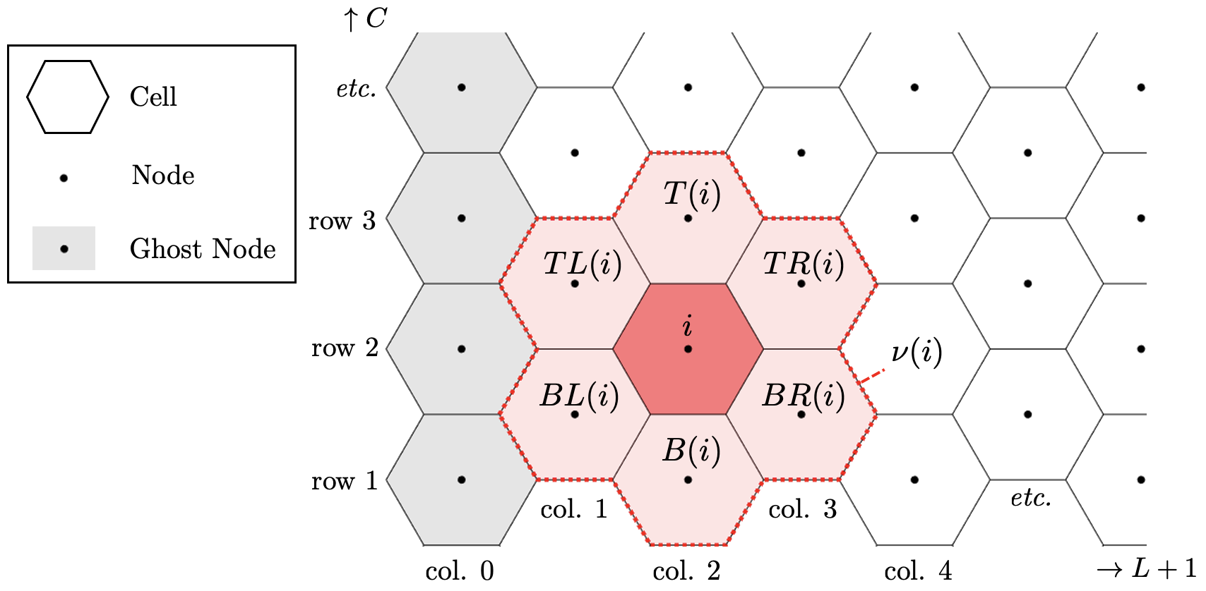
(b)

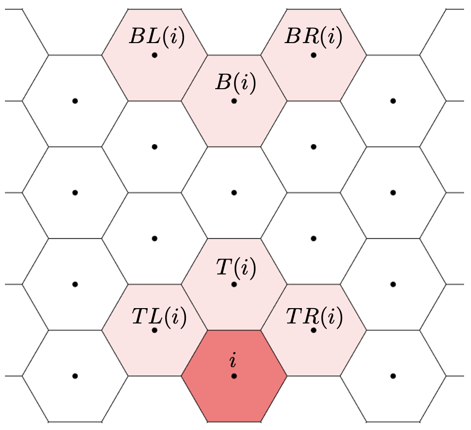
(c)

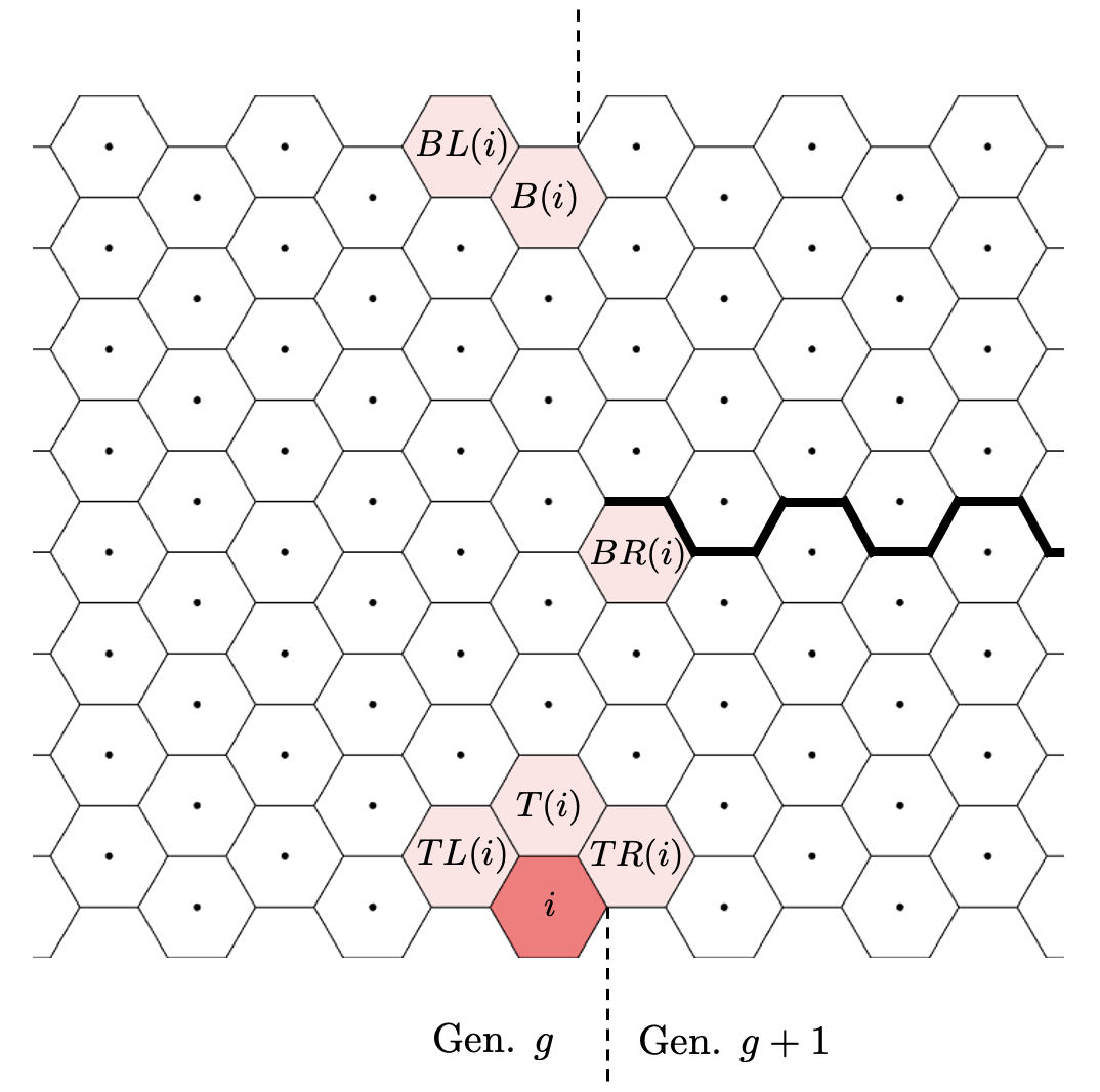
Supplementary Figure S1: (a) Schematic illustrating the notation and methods of the numerical scheme. (b) Adjacency on tube geometry, (c) adjacency on branching geometry

As can be seen in Figure S1, the hexagonal packing of the cells naturally results in the formation of distinct columns of cells, with an offset on alternating columns. To refer to the position of a cell, we adopt the notation $(x(i),y(i))$ to define its position, where $x$ is the column index (counting from the left) and $y$ is the row index (counting from the bottom). We also introduce the inverse notation, $i=n(x,y)$ for the index of the cell in column $x$ and row $y$. With this notation, we can explicitly define the cell adjacency function $\nu(i)$ for different geometries.

For tubes of circumference $C$ cells and length $L$ cells, we represent the unrolled tissue as a rectangular $L\times C$ sheet of cells with periodic boundary conditions in the $y$ direction and no–flux boundary conditions in the $x$ direction. We must assume that $C$ is even to ensure that the hexagonal grid of cells closes; we moreover will always take $L$ to be even. Then for cell $i$, we have

$$\nu(i)=\begin{cases}\left\{T(i),B(i),BR(i),TR(i)\right\},\qquad\qquad\qquad~{}~{}~{}x(i)=1,~{}\text{(left edge)}\\ \left\{BL(i),TL(i),B(i),T(i),BR(i),TR(i)\right\},~{}~{}~{}1<x(i)<L,~{}\text{(tube interior)}\\ \left\{BL(i),TL(i),T(i),B(i)\right\},\qquad\qquad\qquad~{}~{}~{}x(i)=L,~{}\text{(right edge)}\end{cases}$$ (S6)

where $BL(i),~{}TL(i),~{}B(i),~{}T(i),~{}BR(i),~{}TR(i)$ are the bottom-left, top-left, bottom, top, bottom-right, and top-right neighbours of cell $i$, respectively. We have for the tube geometry

$$BL(i) =\begin{cases}n(x(i)-1,R_{\text{\tiny tube}}(y(i)-1)),\qquad~{}~{}x(i)\text{ even,}\\ n(x(i)-1,y(i)),\qquad\qquad\qquad~{}~{}~{}~{}x(i)\text{ odd,}\end{cases}$$ (S7)

$$TL(i) =\begin{cases}n(x(i)-1,y(i)),\qquad\qquad\qquad~{}~{}~{}~{}x(i)\text{ even,}\\ n(x(i)-1,R_{\text{\tiny tube}}(y(i)+1)),\qquad~{}~{}x(i)\text{ odd,}\end{cases}$$ (S8)

$$B(i) =n(x(i),R_{\text{\tiny tube}}(y(i)-1)),$$ (S9)

$$T(i) =n(x(i),R_{\text{\tiny tube}}(y(i)+1)),$$ (S10)

$$BR(i) =\begin{cases}n(x(i)+1,R_{\text{\tiny tube}}(y(i)-1)),\qquad~{}~{}x(i)\text{ even,}\\ n(x(i)+1,y(i)),\qquad\qquad\qquad~{}~{}~{}~{}x(i)\text{ odd,}\end{cases}$$ (S11)

$$TR(i) =\begin{cases}n(x(i)+1,y(i)),\qquad\qquad\qquad~{}~{}~{}~{}x(i)\text{ even,}\\ n(x(i)+1,R_{\text{\tiny tube}}(y(i)+1)),\qquad~{}~{}x(i)\text{ odd,}\end{cases}$$ (S12)

where

$$R_{\text{\tiny tube}}(y)=\texttt{mod}(y-1,C)+1$$

accounts for the periodic boundaries of the tube, where we use the shorthand

$$\texttt{mod}(a,n)=a\mod n.$$

For the branching geometry, under the assumption that branching is even and binary, and that the resulting offspring branches are each half the circumference of the preceding tissue branching generation, we can represent the unrolled tissue as a two-dimensional sheet as follows. We assume that branching tree comprises $G$ tissue generations, such that Generation $h=1,2,...,G$ contains $2^{h-1}$ tubes of cells, and that the circumference of the single tube in Generation 1 is $C$ cells. It follows that the circumference of a tube in a given Generation $h$ is $C/2^{h-1}$ cells. We assume that the overall length of the branching tree from the left to right edges is $L$ cells, and that ${b_{1},b_{2},...,b_{G}}$ are the depths, in numbers of cells from the left edge, of the first cell of each tissue generation, where $b_{1}=1$. As before, we assume that the left and right edges of the branching tree are subject to no–flux boundary conditions.

Under this construction, as for the tube geometry, the general definition of the adjacency function $\nu(i)$ in Equation (S6) remains valid, and we can represent the unrolled branching tree as an $L\times C$ sheet of cells, with the addition of special conditions for cells lying along the boundaries of tube branches. For cell $i$ in a branching tree, we simply adjust the edge reflection terms to obtain the definitions

$$BL(i) =\begin{dcases*}n\left(x(i)-1,R^{\text{\tiny(-)}}_{\text{\tiny branch}}\left(x(i)-1,y(i)-1\right)\right),\qquad~{}~{}x(i)\text{ even,}\\ n(x(i)-1,y(i)),\qquad\qquad\qquad\qquad\qquad\qquad~{}~{}x(i)\text{ odd,}\end{dcases*}$$ (S13)

$$TL(i) =\begin{dcases*}n(x(i)-1,y(i)),\qquad\qquad\qquad\qquad\qquad\qquad~{}~{}x(i)\text{ even,}\\ n\left(x(i)-1,R^{\text{\tiny(+)}}_{\text{\tiny branch}}\left(x(i)-1,y(i)+1\right)\right),\qquad~{}~{}x(i)\text{ odd,}\end{dcases*}$$ (S14)

$$B(i) =n\left(x(i),R^{\text{\tiny(-)}}_{\text{\tiny branch}}\left(x(i),y(i)-1\right)\right),$$ (S15)

$$T(i) =n\left(x(i),R^{\text{\tiny(+)}}_{\text{\tiny branch}}\left(x(i),y(i)+1\right)\right),$$ (S16)

$$BR(i) =\begin{dcases*}n\left(x(i)+1,R^{\text{\tiny(-)}}_{\text{\tiny branch}}\left(x(i)+1,y(i)-1\right)\right),\qquad~{}~{}x(i)\text{ even,}\\ n(x(i)+1,y(i)),\qquad\qquad\qquad\qquad\qquad\qquad~{}~{}x(i)\text{ odd,}\end{dcases*}$$ (S17)

$$TR(i) =\begin{dcases*}n(x(i)+1,y(i)),\qquad\qquad\qquad\qquad\qquad\qquad~{}\ x(i)\text{ even,}\\ n\left(x(i)+1,R^{\text{\tiny(+)}}_{\text{\tiny branch}}\left(x(i)+1,y(i)+1\right)\right),\qquad~{}~{}x(i)\text{ odd,}\end{dcases*}$$ (S18)

where

$$R^{\text{\tiny(-)}}_{\text{\tiny branch}}(x,y)=\begin{cases}y,\qquad\qquad~{}~{}~{}\texttt{mod}(y,c(x))\neq 0,\\ y+c(x),\qquad\texttt{mod}(y,c(x))=0,\end{cases}$$

and

$$R^{\text{\tiny(+)}}_{\text{\tiny branch}}(x,y)=\begin{cases}y,\qquad\qquad~{}~{}~{}\texttt{mod}(y,c(x))\neq 1,\\ y-c(x),\qquad\texttt{mod}(y,c(x))=1,\end{cases}$$

account for the periodic boundaries of the tubes in a given tissue generation. We use the shorthand

$$c(x)=2^{g(x)-1}$$

for the circumference of a tube in column $x$, and

$$g(x)=\max_{h=1,2,...,G}\left\{x\geq b_{h}\right\},$$

for the tissue branching generation of a cell in column $x$.

S4 Tracking lineages

In certain simulated infections, we wish to track multiple viral lineages simultaneously. To account for this, we use the following procedure, which we developed in an earlier publication [9].

Suppose we wish to track $N_{\text{\tiny lin}}$ viral lineages. In what follows, we assume each viral lineage to possess identical infection parameters, however in principle this method could easily be extended to accommodate lineages with differing properties. We begin by augmenting the system to account for infection states specific to each lineage, and a corresponding viral density. Specifically, for each lineage $l=1,2,...,N_{\text{\tiny lin}}$, we denote the latently infected, productively infectious, and dead sub-states associated with that lineage as $E_{l}$, $I_{l}$, and $D_{l}$, respectively. Similarly, if by $\sigma_{i}^{\text{\tiny sub}}(t)$ we denote the sub–state of cell $i$ at time $t$, the viral density of lineage $l$ is given by

$$\frac{\partial v_{l}}{\partial t}=p\sum_{i\in\mathcal{I}_{l}(t)}\frac{\mathbbm{1}_{\left\{S_{i}\right\}}}{\left|S_{i}\right|}-cv_{l}+D\nabla^{2}v_{l},$$ (S19)

where $\mathcal{I}_{l}(t)=\left\{i~{}:~{}\sigma_{i}^{\text{\tiny sub}}(t)=I_{l}\right\}$. Note that $\sum_{i=1}^{N}{}_{\text{\tiny lin}}v_{l}=v$, and that $\mathcal{I}(t)=\cup_{i=1}^{N}{}_{\text{\tiny lin}}\mathcal{I}_{l}(t)$, and so on.

We determine the lineage of a newly infected cell as follows. Assume, following the infection event probability defined in Equation (S2), that cell $i$ is marked to enter the latently infected state during time interval $[t,t+\Delta t)$. The probability that cell $i$ does not enter the $E_{l}$ sub–state during time interval $[t,t+\Delta t)$ is given by

$$P(\sigma_{i}^{\text{\tiny sub}}(t+\Delta t)\neq E_{l}|\sigma_{i}(t+\Delta t)=E,~{} \sigma_{i}(t)=T)$$

$$=P(\mathcal{L}_{i}\neq l)$$

$$=\exp\left(-\left(\alpha\sum_{j\in\nu(i)}\frac{\mathbbm{1}_{\left\{\sigma_{j}(t)=I_{l}\right\}}}{\left|\nu(i)\right|}+\beta V_{l}\right)\Delta t\right),$$ (S20)

where the more convenient notation $P(\mathcal{L}_{i}\neq l)$ has the obvious definition. Therefore, we determine the probability that cell $i$ is infected with lineage $l$ as

$$P(\mathcal{L}_{i}=l)=\frac{1-P(\mathcal{L}_{i}\neq l)}{\sum_{m=1}^{N_{\text{\tiny lin}}}\left(1-P(\mathcal{L}_{i}\neq m)\right)}.$$ (S21)

We then assign viral lineage as follows. First, draw a random number $x\sim~{}Uniform(0,1)$, then compute

$$l^{*}=\min\left\{l~{}:~{}x<\sum_{m=1}^{l}{P(\mathcal{L}_{i}=m)}\right\},$$ (S22)

that is, the minimum $l$ such that the probability of cell $i$ having a lineage of at most $l$ is greater than $x$. Cell $i$ is then assigned lineage $l^{*}$.

S5 Numerical methods

We simulate our model by stepping time in increments of length $\Delta t$ (throughout this work, we use $\Delta t=0.01\text{h}$). At a given time $\tau$, we denote by $\mathcal{G}^{\tau}$ the state of the cell grid, and by $v_{\cdot}^{\tau}$ the discretised form of the viral density surface $v(\cdot,\tau)$. Then, during the time step $[\tau,\tau+\Delta t)$, we perform the following.

Firstly, following the state transition probabilities in Equations (S2)–(S1), we check each cell for a state transition, and generate the cell grid for the next time step, $\mathcal{G}^{\tau+\Delta t}$, based on the state of the cell grid and viral density surface at the start of the time step, that is, $\mathcal{G}^{\tau}$ and $v_{\cdot}^{\tau}$, respectively.

We then update the discretised viral surface using an implicit–explicit finite–difference scheme. We discretise the viral density in space such that the cells themselves may be considered the nodes of the discretised surface. As a consequence, the total viral density at cell $i$ at time $\tau$ is trivially computed as

$$\int_{S_{i}}v(\mathbf{x},\tau)d\mathbf{x}=v_{i}^{\tau},$$

where $v_{i}^{\tau}$ is the value of the discretised viral surface at node (cell) $i$. In an earlier work, we discussed the discretisation of such viral surfaces, and found that when diffusion is sufficiently large compared to the length scale of the cell, discretisation at the cell scale was sufficient to ensure convergence of the virus PDE [8]. Throughout this work, we employ very rapid diffusion compared to the length scale of the cell (by default, $100~{}\text{CD}^{2}\text{h}^{-1}$), which justifies this choice of discretisation.

For the viral diffusion, we use a Backwards–Euler method constructed on the hexagonal lattice of nodes (cells). Since we use no–flux boundary conditions on the left and right edges of the tissue, we introduce $C$ additional ghost nodes on both the left and right edges of the tissue in columns 0 and $L+1$, following the notation introduced above. We extend the definition of the functions $n(x,y)$, $x(i)$ and $y(i)$ to also assign a single index $i=N+1,N+2,...,N+2C$ to ghost node $g_{i}$ residing at position $(x,y)$ and vice versa, and define the new adjacency function

$$\nu^{*}(i)=\nu(i)\cup\nu_{\text{\tiny edge}}(i),$$ (S23)

on $i=1,2,...,N$, that is, for the cell nodes, where

$$\nu_{\text{\tiny edge}}(i)=\begin{cases}\left\{TL(i),BL(i)\right\},\qquad\qquad x(i)=1,~{}~{}\text{(left edge)}\\ \emptyset,\qquad\qquad\qquad\qquad\qquad~{}1<x(i)<L,\\ \left\{BR(i),TR(i)\right\},\qquad~{}~{}~{}~{}~{}x(i)=L.~{}~{}\text{(right edge)}\end{cases}$$

Then, on $i=N+1,N+2,...,N+2C$ — that is, for the ghost nodes — define

$$\nu_{\text{\tiny ghost}}^{\text{\tiny col}}(i)=\left\{T(i),B(i)\right\},$$

and

$$\nu_{\text{\tiny ghost}}^{\text{\tiny int}}(i)=\begin{cases}\left\{BR(i),TR(i)\right\},\qquad\qquad x(i)=0,~{}~{}\text{(left ghosts)}\\ \left\{TL(i),BL(i)\right\},\qquad\qquad x(i)=L+1.~{}~{}\text{(right ghosts)}\end{cases}$$

for the neighbours of the ghost nodes lying in the ghost column, and in the interior of the node grid, respectively.

Overall, the scheme for the update step is given by the matrix equation

$$\hat{\mathbf{v}}_{\text{\tiny imp}}^{\tau+\Delta t}=\mathbf{D}^{-1}\hat{\mathbf{v}}^{\tau},$$ (S24)

where

$$\hat{\mathbf{v}}^{\tau}=\left\{\mathbf{v}^{\tau},\mathbf{g}^{\tau}\right\}=\left\{v_{1}^{\tau},v_{2}^{\tau},...,v_{N}^{\tau},g_{N+1}^{\tau},g_{N+2}^{\tau},...,g_{N+2C}^{\tau}\right\},$$ (S25)

and $\mathbf{D}$ is the $(N+2C)\times(N+2C)$ discretised diffusion matrix, which reflects the adjacency structure of the nodes, such that

$$\mathbf{D}_{i,j}=\begin{dcases}(1+\frac{4D\Delta t}{\Delta x^{2}}),\qquad i=j,~{}j=1,2,...,N+2C,\\ -\frac{2}{3}\frac{D\Delta t}{\Delta x^{2}},\qquad~{}~{}~{}~{}i\in\nu^{*}(j),~{}j=1,2,...,N,\\ -\frac{2}{3}\frac{D\Delta t}{\Delta x^{2}},\qquad~{}~{}~{}~{}i\in\nu_{\text{\tiny ghost}}^{\text{\tiny col}}(j),~{}j=N+1,N+2,...,N+2C,\\ -\frac{4}{3}\frac{D\Delta t}{\Delta x^{2}},\qquad~{}~{}~{}~{}i\in\nu_{\text{\tiny ghost}}^{\text{\tiny int}}(j),~{}j=N+1,N+2,...,N+2C,\\ 0,\qquad\qquad\qquad~{}~{}\text{otherwise}.\end{dcases}$$

Here, $\Delta x$ is the distance between cell centres (cell diameter, or CD). Throughout this work, we work in units of CD, and hence take $\Delta x=1$. In an update step, we compute the value of the discretised virus surface at time $\tau+\Delta t$ using Equation (S24) (in practice, we use sparse system solvers instead of the computationally expensive process of finding the inverse of $\mathbf{D}$). We then set $g_{n(0,y)}^{\tau+\Delta t}=v_{n(1,y)}^{\tau+\Delta t}$, $g_{n(L+1,y)}^{\tau+\Delta t}=v_{n(L,y)}^{\tau+\Delta t}$ for $y=1,2,...,C$ to account for the no–flux boundary conditions.

Note that this method only really depends on the definition of the cell adjacency function $\nu$, meaning it applies to the definitions for both the tube and branching tree geometries we have described (and in fact more generally). We skirt potential complexities arising from the complex topology of the sheet by essentially approximating the continuous viral diffusion process as a discrete, cell-based process.

Having computed the viral diffusion step, we then apply an explicit scheme for the remaining terms of the virus PDE:

$$\mathbf{v}_{\text{\tiny exp}}^{\tau+\Delta t}=\mathbf{v}^{\tau}+\Delta t\left(p\mathbf{I}^{\tau}-c\mathbf{v}^{\tau}\right),$$ (S26)

where

$$\mathbf{I}^{t}=\left\{\frac{\mathbbm{1}_{\left\{\sigma_{1}(t)=I\right\}}}{N\left|S_{1}\right|},\frac{\mathbbm{1}_{\left\{\sigma_{2}(t)=I\right\}}}{N\left|S_{2}\right|},...,\frac{\mathbbm{1}_{\left\{\sigma_{N}(t)=I\right\}}}{N\left|S_{N}\right|}\right\}.$$

The final update step, then, is given by

$$\mathbf{v}^{\tau+\Delta t}=\mathbf{v}_{\text{\tiny imp}}^{\tau+\Delta t}+\mathbf{v}_{\text{\tiny exp}}^{\tau+\Delta t}.$$ (S27)

S6 Immune response parameter sweep — choice of contours

Supplementary Figure S2: $F^{\infty}$ contours on $t_{\text{\tiny act}}$–$F^{\text{\tiny thresh}}$ space for infections of the branching tree seeded in Generation 1 or 5. Immune parameters as defined in the main text.

S7 Anatomically accurate lung dimensions

(a)

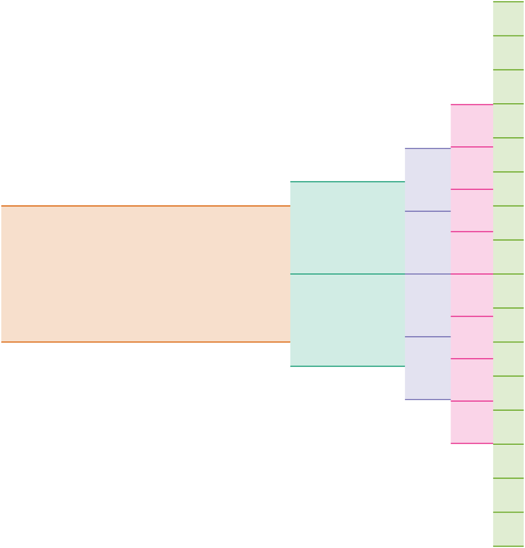
(b)

Supplementary Figure S3: Unwrapped airway tissue dimensions based on experimental measurements on the human respiratory tree [5], where we take five consecutive generations from (a) the top of the respiratory tree and (b) the terminal five generations before the alveolar sacs.

References

- Beauchemin et al., [2006] Beauchemin, C., Forrest, S., and Koster, F. T. (2006). Modeling influenza viral dynamics in tissue. In Bersini, H. and Carneiro, J., editors, Artificial Immune Systems, pages 23–36, Berlin, Heidelberg. Springer Berlin Heidelberg.
- Fain and Dobrovolny, [2022] Fain, B. G. and Dobrovolny, H. M. (2022). GPU acceleration and data fitting: Agent-based models of viral infections can now be parameterized in hours. Journal of Computational Science, 61:101662.
- Holder et al., [2011] Holder, B. P., Liao, L. E., Simon, P., Boivin, G., and Beauchemin, C. A. A. (2011). Design considerations in building in silico equivalents of common experimental influenza virus assays. Autoimmunity, 44(4):282–293.
- Kongsomros et al., [2021] Kongsomros, S., Manopwisedjaroen, S., Chaopreecha, J., Wang, S.-F., Borwornpinyo, S., and Thitithanyanont, A. (2021). Rapid and efficient cell-to-cell transmission of avian influenza H5N1 virus in MDCK cells is achieved by trogocytosis. Pathogens, 10(4).
- Makevnina, [2018] Makevnina, V. V. (2018). Solid-state modeling of human tracheobronchial tree for 23 generations of airways. Journal of Physics: Conference Series, 1124(3):031002.
- Petrie et al., [2013] Petrie, S. M., Guarnaccia, T., Laurie, K. L., Hurt, A. C., McVernon, J., and McCaw, J. M. (2013). Reducing uncertainty in within-host parameter estimates of influenza infection by measuring both infectious and total viral load. PLOS ONE, 8(5):e64098–.
- Sego et al., [2020] Sego, T. J., Aponte-Serrano, J. O., Gianlupi, J. F., Heaps, S. R., Breithaupt, K., Brusch, L., Crawshaw, J., Osborne, J. M., Quardokus, E. M., Plemper, R. K., and Glazier, J. A. (2020). A modular framework for multiscale, multicellular, spatiotemporal modeling of acute primary viral infection and immune response in epithelial tissues and its application to drug therapy timing and effectiveness. PLOS Computational Biology, 16(12):e1008451.
- Williams et al., [2023] Williams, T., McCaw, J. M., and Osborne, J. M. (2023). Choice of spatial discretisation influences the progression of viral infection within multicellular tissues. Journal of Theoretical Biology, 573:111592.
- Williams et al., [2024] Williams, T., McCaw, J. M., and Osborne, J. M. (2024). Spatial information allows inference of the prevalence of direct cell–to–cell viral infection. PLOS Computational Biology, 20(7):1–35.
- Zeng et al., [2022] Zeng, C., Evans, J. P., King, T., Zheng, Y.-M., Oltz, E. M., Whelan, S. P. J., Saif, L. J., Peeples, M. E., and Liu, S.-L. (2022). SARS-CoV-2 spreads through cell-to-cell transmission. Proceedings of the National Academy of Sciences, 119(1):e2111400119.