Prophet Inequalities: Competing with the Top $\ell$ Items is Easy

Abstract

We explore a novel variant of the classical prophet inequality problem, where the values of a sequence of items are drawn i.i.d. from some distribution, and an online decision maker must select one item irrevocably. We establish that the competitive ratio between the expected optimal performance of the online decision maker compared to that of a prophet, who uses the average of the top $\ell$ items, must be greater than $\ell/c_{\ell}$, with $c_{\ell}$ the solution to an integral equation. We prove that this lower bound is larger than $1-1/(\exp(\ell)-1)$. This implies that the bound converges exponentially fast to $1$ as $\ell$ grows. In particular, the bound for $\ell=2$ is $2/c_{2}\approx 0.966$ which is much closer to $1$ than the classical bound of $0.745$ for $\ell=1$. Additionally, the proposed algorithm can be extended to a more general scenario, where the decision maker is permitted to select $k$ items. This subsumes the $k$ multi-unit i.i.d. prophet problem and provides the current best asymptotic guarantees, as well as enables broader understanding in the more general framework. Finally, we prove a nearly tight competitive ratio when only static threshold policies are allowed.

1 Introduction

Decision makers are frequently confronted to the arduous task of making crucial decisions with limited information. When a seller wants to sell a limited number of items to a stream of customers, potential future customers with a high willingness to pay must be taken into account. How long should the seller wait before finally lowering its expectations, and to what price? Is the current customer likely to be the best we can hope to interact with? This common challenge is at the heart of many online selection problems (Borodin and El-Yaniv, 1998), with some of the most simplest and famous version of this online selection problem being the secretary problem for adversarial inputs (Ferguson, 1989), and prophet inequalities for random inputs (Correa et al., 2019b), which is the focus of this work.

A classical way of measuring the performance of an online decision problem is to consider the so-called competitive ratio, which the worst-case ratio between the performance of an online algorithm and that of a benchmark that has usually access to more information than the decision maker. This has been the focus of many works, in online matching (Mehta, 2013), scheduling (Motwani et al., 1994), or metrical tasks systems (Bubeck et al., 2018) to name but a few, where explicit upper and lower bound on the competitive ratio were provided. This type of metric makes it possible to design robust algorithms, that are able to always perform approximately well in any circumstances.

The classical prophet inequality dates back to the $1970s$, with Krengel and Sucheston (1977) famously showing that a gambler allowed to select a single item using an optimal online algorithm can always recover at least half of the item value chosen by an omniscient prophet able to see the future, this $1/2$ factor being the best possible. Following this, Samuel-Cahn (1984) proved that a simple threshold algorithm can actually achieve this competitive ratio of $1/2$. The full prophet region was characterized by Hill (1983) which showed that for bounded random variables and $V$ the expected optimal value of the gambler, then the expected maximum is always smaller than $2V-V^{2}$.

Following these works, variations with different assumptions on the item distributions were considered. If there are no assumptions on the joint distribution of the sequence of values, then Hill and Kertz (1983) showed that the worst-case comparison between the gambler and the prophet can be arbitrarily bad in the number of items. Conversely, assumptions on the joint distribution can be strengthened: Hill and Kertz (1982) are the first to consider the Independent and Identically Distributed (i.i.d.) setting, in which the values of all items are independently drawn from the same distribution. An implicit upper bound of approximately $0.745$ on the competitive ratio was proposed by Kertz (1986a) which reduces the computation of the worst-case competitive ratio to a finite dimensional optimization problem. This upper bound was proven to be tight by Correa et al. (2017) through the construction of an explicit adaptive quantile algorithm that achieves this bound, showing that the worst-case competitive ratio in the i.i.d. setting is exactly the solution to an integral equation (with a numerical value of around $0.745$). Some other works have further investigated the i.i.d. case, with Perez-Salazar et al. (2022) showing that this optimal competitive ratio can be achieved with fewer different thresholds, and Jiang et al. (2022) showing as a special case that the result of a specific optimization problem yields a value arbitrarily close to the worst-case optimization problem, although it only outputs a guarantee for a fixed number of items.

One important observation is that the worst-case instances tend to involve distributions that depend on the number of items and have a particularly heavy tail, which does not correspond to the most commonly encountered distributions. In particular, for most distributions, the optimal online algorithm tend to perform better than what the worst-case instance suggests. As a result, some authors propose to use a different benchmark. Kennedy (1985) and Kertz (1986b), for instance, studied the competitive ratio when the comparison is made with respect to a weaker prophet that receives the average reward of the top $\ell$ items. They prove that, in the case where valuation are independent but not necessarily identically distributed, the competitive ratio of any online algorithm cannot be larger than $1-\ell/(\ell+1)$, and that this bound is attained. In this work, we consider the same benchmark of Kennedy (1985); Kertz (1986b), but with i.i.d. valuations as in Hill and Kertz (1982); Kertz (1986a); Correa et al. (2017). We prove a lower bound on the competitive ratio and provide an efficient quantile algorithm to solve the problem.

Contributions

We consider a setting with $n\in\mathbb{N}$ items whose valuations are $(X_{1},\dots,X_{n})$. The variables $(X_{i})_{i\geq 1}$ are i.i.d. non-negative random variables drawn according to some distribution $F$, and we denote by $X_{(1)}\geq\dots X_{(n)}$ their order statistics. We consider online algorithms that observe the valuations sequentially and selects exactly one item (out of $n$ items). The algorithm works in an online fashion and makes irrevocable decisions: for an item $i$, the algorithm observes its valuation $X_{i}$ and must decide whether to select item $i$ or move to the next item. As a result, an algorithm induces a stopping time $\tau$, that corresponds to the item selected and its performance is $E[X_{\tau}]$. We will compare the performance of an algorithm to the average valuation of the top $\ell$ items, $\mathbb{E}_{X\sim F}[\ell^{-1}\sum_{i\in[\ell]}X_{(i)}]$. For $n$ and $\ell$, we define the competitive ratio as:

$$\operatorname{CR}_{\ell}(n)=\inf_{F}\sup_{\tau\text{ stopping time}}\frac{\mathbb{E}_{X\sim F}[X_{\tau}]}{\mathbb{E}_{X\sim F}\left[\frac{1}{\ell}\sum_{i\in[\ell]}X_{(i)}\right]}.$$ (1)

This corresponds to the competitive ratio achievable by an algorithm that knows the distribution $F$. Note that we always have $\operatorname{CR}_{\ell}(n)\leq 1$ by taking a constant distribution $X_{i}=1$.

Our first result is the following lower bound on the competitive ratio:

Theorem 1.

For all positive integers $\ell$, we have:

$$\operatorname{CR}_{\ell}\vcentcolon=\inf_{n\geq\ell}\operatorname{CR}_{\ell}(n)\geq\frac{\ell}{c_{\ell}},$$ (2)

where $c_{\ell}$ is defined as the unique solution in $[\ell,\infty)$ to the integral equation

$$\frac{1}{(\ell-1)!}\int_{0}^{\infty}\frac{\nu^{{\ell}-1}}{e^{\nu}(c_{\ell}-{\ell})+{\ell}\sum_{i=0}^{{\ell}}\frac{\nu^{i}}{i!}}d\nu=1.$$ (3)

Our analysis is based on a non-trivial generalization of the quantile algorithm presented in Correa et al. (2017). By using properties of Beta functions, we show that maximizing the parameter of the proposed quantile algorithm Algorithm 1 is equivalent to solving a non-linear discrete boundary value problem. We then show that this discrete boundary value problem corresponds to a continuous boundary value problem in the limit where $n$ goes to infinity. This limiting competitive ratio lower bound yields the integral equation (3). Finally, we prove that the competitive ratio for a finite $n$ is bounded by its limits as $n$ grows, which provide a guarantee on the quantile algorithm.

$\ell$	1	2	3	4	5
Lower bound $\ell/c_{\ell}$	0.745	0.966	0.997	0.9998	0.999993

Table 1: First digits of the lower bound $\ell/c_{\ell}$.

There are no explicit solutions to the integral equation (3), but this equation can be easily solved numerically. We report the first values of the competitive ratio $\ell/c_{\ell}$ in Table 1. In the special case $\ell=1$, we recover the integral equation of Kertz (1986a); Correa et al. (2017), which corresponds to the lower bound of $0.745$ for the classical i.i.d. prophet. What is striking is that for $\ell\geq 2$, the competitive ratio increases extremely fast towards $1$. In particular, for $\ell=2$, the competitive ratio is larger than $0.966$, which is much closer to $1$ than $0.745$. For any distribution $F$, one has:

$$\sup_{\tau\text{ stopping time}}\mathbb{E}[X_{\tau}] \geq 0.745~{}\mathbb{E}[X_{(1)}]$$ (result of Correa et al. (2017))

$$\sup_{\tau\text{ stopping time}}\mathbb{E}[X_{\tau}] \geq 0.966~{}\mathbb{E}[\frac{1}{2}(X_{(1)}+X_{(2)})]$$ (our bound)

The main reason is that the worst-case instances for $\ell=1$ rely on the first and second maximum being very different. In fact, such an instance is relatively easy when using the benchmark $(X_{(1)}+X_{(2)})/2$. We observe numerically that $\ell/c_{\ell}$ grows exponentially fast to $1$ (roughly of of the order of $1-10^{-\ell}$). Our second main result is to show that indeed the competitive ratio provably converges exponentially fast to $1$ as $\ell$ grows:

Theorem 2.

For all positive integers $\ell$, we have:

$$\operatorname{CR}_{\ell}\geq 1-\frac{1}{e^{\ell}-1}.$$ (4)

Note that this bound is not as tight as the one suggested in Table 1 but still provides the exponential convergence rate to $1$. Compared to the tight competitive ratio of $1-1/(\ell+1)$ in Kennedy (1985) without the i.i.d. assumption, the convergence towards $1$ is noticeably faster. This exponential convergence rate explains why the jump from $\ell=1$ to $\ell=2$ was so marked. This is the first result in prophet inequalities with an exponential convergence rate towards $1$.

All of our results are obtained through a quantile algorithm which is known to have additional benefits, such as being more amenable to a learning setting (Rubinstein et al., 2019) and being potentially easy to compute and implement in instances where the distribution is hard to integrate but can be still be accessed punctually.

We also show that our algorithm can be extended with provable guarantees to a more general setting introduced by Kennedy (1987) for the non i.i.d. case, where the decision maker is allowed to select $k$ items, which subsumes the $k$ multi-unit (Alaei, 2011; Jiang et al., 2022) i.i.d. prophet problem when $\ell=k$. An algorithm that sequentially selects $k$ items will induce a sequence of stopping time $(\tau_{i})_{i\in[k]}$, for which if $\tau_{i}<\infty$ then $\tau_{i}<\tau_{i+1}$. We thus consider the following competitive ratio:

$$\operatorname{CR}_{k,\ell}(n)=\inf_{F}\sup_{\tau_{1}<\dots<\tau_{k}}\frac{\mathbb{E}_{X\sim F}\left[\frac{1}{k}\sum_{i\in[k]}X_{\tau_{i}}\right]}{\mathbb{E}_{X\sim F}\left[\frac{1}{\ell}\sum_{i\in[\ell]}X_{(i)}\right]}.$$ (5)

We prove asymptotic guarantees on $\operatorname{CR}_{k,\ell}(n)$.

Theorem 3.

For all positive integers $k$ and $\ell$, we have:

$$\liminf_{n\rightarrow\infty}\operatorname{CR}_{k,\ell}(n)\geq\frac{\ell}{k}\sum_{j\in[k]}\frac{1}{c_{\ell}}\frac{1}{\prod_{t\in[j]}\theta_{j,\ell}},$$ (6)

where $\theta_{1,\ell}=1$ and $c_{1,\ell},\theta_{2,\ell},\dots,\theta_{k,\ell}$ are the unique parameters such that the following boundary value problem admits a solution,

$$\frac{db^{1}(t)}{dt} =c_{1,\ell}-\ell\cdot\gamma_{\ell+1}\circ\gamma_{\ell}(b^{j}(t)),$$

$$\frac{db^{j}(t)}{dt} =\ell\left(\theta_{j,\ell}\cdot\gamma_{\ell+1}\circ\gamma_{\ell}^{-1}(b^{j-1}(t))-\gamma_{\ell+1}\circ\gamma_{\ell}(b^{j}(t))\right),\quad 2\leq j\leq k$$ for (7)

$$b^{j}(0) =0,\quad b^{j}(1)=1,\quad \text{for $1\leq j\leq k$},$$

where $\gamma_{x}(t)$ and $\gamma_{x}^{-1}(t)$ are respectively the cumulative distribution function and the quantile function from a $\mathrm{Gamma}(x,1)$ random variable evaluated at $t$.

Finally, we extend the analysis to the setting where the decision maker is restricted to use static thresholds policies. When the decision maker and the prophet must select $k$ and $\ell$ items respectively and the decision maker is restricted to static threshold policies we define the competitive ratio as

$$\operatorname{CR}_{k,\ell}^{S}(n)=\inf_{F}\sup_{T}\frac{\mathbb{E}_{X\sim F}\left[\frac{1}{k}\sum_{i\in[k]}X_{T_{i}}\right]}{\mathbb{E}_{X\sim F}\left[\frac{1}{\ell}\sum_{i\in[\ell]}X_{(i)}\right]},$$ (8)

where the $T_{i}$ are the stopping times induced by the static threshold $T\in\mathbb{R}^{+}$ which selects an item whenever $T\geq X$.

Using intermediary results derived for Theorems 1 and 3 and extending some of the analysis from Correa et al. (2019b) and Arnosti and Ma (2021) we nearly characterize the exact competitive ratio for static thresholds:

Theorem 4.

For all positive integers $k$ and $\ell$, and $n\geq\max(k,\ell)$, we have:

$$\left|\operatorname{CR}^{S}_{k,\ell}(n)-\frac{\sum_{j=1}^{k}\Pr(\mathrm{Gamma}(j,1)\leq\ell)}{k}\right|\leq O\left(\frac{1}{n}\right).$$ (9)

This result recovers a special case of the tight static threshold competitive ratio provided in Arnosti and Ma (2021) when $n\rightarrow\infty$ and with i.i.d. valuations, but is on other aspects more general by allowing for $\ell\neq k$.

Roadmap

The rest of the paper is organized as follows. In Section 2, we present the quantile algorithm and the analysis of the competitive ratio for finite $n$. In Section 3 we show how to use the limit performance guarantees (as the number of items $n$ goes to infinity) to construct the ODE and derive Theorem 1 and Theorem 2. We provide a numerical analysis of the tightness of the bound in Section 4. In Section 5 we show how to extend our algorithm to the selection of $k$ items and construct a corresponding system of $k$ ODE to obtain Theorem 3. Section 6 deals with the static threshold setting and proves Theorem 4. The detailed proofs of all results are presented in Section 7. Finally, some additional related work is presented in Section 8.

2 Competitive ratio guarantees for a given number of items

The formulation of an optimal online algorithm through the optimal stopping time, as in (1), makes difficult the analysis of the competitive ratio. In this section, we construct an explicit algorithm, and we derive an analysis of the competitive ratio of this algorithm. This algorithm builds on quantiles of the Beta distribution.

For the remainder of the paper and for simplicity of notations, we will consider that $F$ is absolutely continuous with respect to the Lebesgue measure and admits a density $f\geq 0$. , The function $F$ is the cumulative distribution function $F(x)=\Pr(X\leq x)$, and we denote by $F^{-1}$ its quantile function: for each $p\in[0,1]$, $F^{-1}(p)=\inf\{x\in\mathbb{R}\mid p\leq F(x)\}$. Most quantities depend on $n$ and this will be omitted, except punctually when this makes the understanding clearer and will be denoted as $x(n)$ for some quantity $x$.

2.1 The quantile algorithm

We define the quantile algorithm Algorithm 1, which takes as an input the known distribution $F$, and an increasing sequence $0=\epsilon_{0}<\dots<\epsilon_{n}=1$. For each item $i$, this algorithm samples a quantile $q_{i}$ from a Beta($\ell,n-\ell$) distribution truncated to $\epsilon_{i-1}$ and $\epsilon_{i}$ and selects item $i$ if and only if $F(X_{i})\geq 1-q_{i}$. We will denote by $\operatorname{ALG}_{n}$ the expected performance of the algorithm for a sequence of $n$ items. This generalizes the quantile algorithm described in Correa et al. (2017) for the special case $\ell=1$, and no mentions of Beta distributions were made.

Algorithm 1 Quantile algorithm for $\ell$

Input: Partition $(\epsilon_{i})_{0\leq i\leq n}$ of $[0,1]$, distribution $F$ of the $X_{i}$.

for $i\in[n]$: do

     Draw $q_{i}$ from $\mathrm{Beta}(\ell,n-\ell)$ truncated between $\epsilon_{i-1}$ and $\epsilon_{i}$

     if $X_{i}\geq F^{-1}(1-q_{i})$: then

         Accept item $i$ and stop

     end if

end for

Before showing a bound on the performance of the algorithm, we introduce some notations regarding the Beta distribution. We recall that the density of a $\mathrm{Beta}(\ell,n-\ell)$ random variable is equal to

$$\psi_{\ell,n-\ell}(x)=\frac{x^{\ell}(1-x)^{n-\ell}}{B(\ell,n-\ell)},$$ (10)

where $B(\ell,n-\ell)\vcentcolon=(\ell-1)!(n-\ell-1)!/(n-1)!$ is the normalization constant. As $q_{i}$ is drawn from a distribution truncated between $\epsilon_{i-1}$ and $\epsilon_{i}$, we denote the normalizing factor of this $\psi_{\ell,n-\ell}$ truncated distribution by $\alpha_{i}=\int_{\epsilon_{i-1}}^{\epsilon_{i}}\psi_{\ell,n-\ell}(x)dx$. Finally, we denote by $a_{i}\vcentcolon=\alpha_{i}\mathbb{E}[(1-q_{i})]$, where $\mathbb{E}[(1-q_{i})]$ is the expected probability of not selecting item $i$ when observing it.

Our first result provides a bound on the performance of Algorithm 1 (valid for any sequence of $\epsilon_{i}$s), as a function of the quantities $\alpha_{i}$ and $a_{i}$ defined above.

Proposition 1.

For $\operatorname{OPT}_{\ell,n}=\mathbb{E}[\sum_{i\in[\ell]}X_{(i)}]$ and $\rho_{i}=\alpha_{i}^{-1}\prod_{j=1}^{i-1}a_{j}/\alpha_{j}$, we have the inequality

$$\frac{\min_{i\in[n]}\rho_{i}}{n}\operatorname{OPT}_{\ell,n}\leq\operatorname{ALG}_{n}\leq\frac{\max_{i\in[n]}\rho_{i}}{n}\operatorname{OPT}_{\ell,n}.$$ (11)

Sketch of proof.

The proof decomposes in two steps. First, we compute an expression of $\operatorname{ALG}_{n}$: remarking that the quantiles $q_{i}$ are independent, we can show that the performance of $\operatorname{ALG}_{n}$ is equal to $\sum_{i\in[n]}\rho_{i}\int_{\epsilon_{i-1}}^{\epsilon_{i}}\psi_{\ell,n-\ell}(q)dq$. Second, we derive an expression for $\operatorname{OPT}_{\ell,n}$ as an expectation of the function $R(Q)$, where $R(q)$ is the expected reward of accepting an item with threshold $F^{-1}(1-q)$ and $Q$ is some random variable. In Correa et al. (2017), the distribution of $Q$ was shown to be the density $(n-1)(1-q)^{n-2}$ in the special case $\ell=1$. We prove by using the density for a general order statistic, that the right density in the case $\ell>1$ is $\psi_{\ell,n-\ell}$. Because $\operatorname{OPT}_{\ell,n}=n\mathbb{E}_{q\sim\psi_{\ell,n-\ell}}[R(q)]$, we can take the minimum or the maximum over the $\rho_{i}$ to obtain (11). A full proof is provided in Section 7.1. ∎

This result implies that if we construct a sequence of $\epsilon$ such that $\min_{i\in[n]}\rho_{i}=\max_{i\in[n]}\rho_{i}$, then the competitive ratio of the algorithm will be exactly $\rho_{i}/n$. This is what we use in the following.

2.2 Optimizing the parameters of the algorithm

Looking at Proposition 1, we see that the $\rho_{i}$s are functions of $\epsilon_{i}$. A lower bound on the performance of the algorithm is therefore obtained if we can find the sequence $\epsilon_{i}$ which maximizes $\min_{i\in[n]}\rho_{i}$. A natural choice of $\epsilon_{i}$ would be to find a sequence such that all the $\rho_{i}$ are equal, this would lead to an algorithm whose performance is exactly $(\max_{i}\rho_{i}/n)\operatorname{OPT}_{n}$. It is, however, not clear whether such a sequence of $\epsilon_{i}$ exists, and in particular, because we need this sequence of $\epsilon$ to be increasing (i.e., $\epsilon_{i-1}<\epsilon_{i}$) for the algorithm to be well defined.

We will first see that finding the $\epsilon_{i}$ such that $\rho_{i}=\rho_{i+1}$ is equivalent to solving a discrete boundary value problem on a non-linear transformation of the $\epsilon_{i}$ by an incomplete beta function, and then use this transformed problem to prove the existence of such $\epsilon_{i}$.

We introduce the variables $b_{i}=\beta_{\ell,n-\ell}(\epsilon_{i})$ which is a nonlinear transformation of $\epsilon_{i}$, where

$$\beta_{\ell,n-\ell}(x)=\frac{\int_{0}^{x}t^{\ell-1}(1-t)^{n-\ell-1}dt}{B(\ell,n-\ell)}.$$ (12)

is actually the cumulative distribution function of $\psi_{\ell,n-\ell}$, also called the regularized incomplete beta function.

Because $\beta_{\ell,n-\ell}$ is strictly monotone as a distribution function with an associated positive density, it has an inverse, and we can recover $\epsilon_{i}$ with $\beta^{-1}_{\ell,n-\ell}(b_{i})$. We also define the discrete difference operator $\Delta$, with $\Delta[b_{i}]=b_{i+1}-b_{i}$. It is the discrete analogue of the continuous differentiation operator. Similarly, we define $\Delta^{2}[b_{i}]=\Delta[\Delta[b_{i}]]=b_{i+2}-2b_{i+1}-b_{i}$.

Lemma 1.

All the $\rho_{i}$ are equal if and only if the following difference equation holds for all $b_{i}$:

$$\Delta[b_{i}]=-\frac{\ell}{n}\beta_{\ell+1,n-\ell}\circ\beta^{-1}_{\ell,n-\ell}(b_{i})+b_{1}.$$ (13)

Sketch of proof.

The main idea is that we can actually express $\alpha_{i}$ and $a_{i}$ in terms of $\beta_{\ell,n-\ell}$, indeed $\alpha_{i}=\beta_{\ell,n-\ell}=\beta_{\ell,n-\ell}(\epsilon_{i})-\beta_{\ell,n-\ell}(\epsilon_{i-1})=b_{i}-b_{i-1}$, and after some computation it can be showed that $a_{i}=(n-\ell)(\beta_{\ell,n+1-\ell}(\epsilon_{i})-\beta_{\ell,n+1-\ell}(\epsilon_{i-1}))/n$. Then using that there is an exact recurrence relationship between $\beta_{\ell,n+1-\ell}$ and $\beta_{\ell,n-\ell}$, as well as between $\beta_{\ell+1,n-\ell}$ and $\beta_{\ell,n-\ell}$, we can obtain a non-linear second order difference equation. Then, for every $i\geq 2$, it is sufficient to sum these difference equations for all $j\leq i$, to obtain a recurrence relation directly on the $b_{i}$. The full proof can be found in Section 7.2. ∎

Note that obtaining an explicit recurrence relation of $\epsilon_{i+1}$ with ‘simple’ functions of the previous $\epsilon_{i}$ is difficult: it can be seen that developing the integrals to obtain such a relation yields an implicit polynomial equation in $\epsilon_{i+1}$ parameterized by $\epsilon_{i}$. This would entail solving a sequence of polynoms of degree $n-\ell+1$. The approach that we use here is to obtain an explicit recurrence relation on a non-linear transformation of the $\epsilon_{i}$ (the $b_{i}$), and not on the $\epsilon_{i}$ themselves. This non-linear transformation has no inverse expressible with ‘simple’ functions exactly whenever $\ell\geq 2$; this explains why the task is considerably more difficult than for the case $\ell=1$ studied in Correa et al. (2017). This difficulty is one of the core obstacles to an extension of the work of Correa et al. (2017).

This recurrence relation (13) also yields a recurrence relation on $\epsilon_{i}$ that involves $\beta_{\ell,n-\ell}^{-1}$ (which does not have an explicit expression except when $\ell=1$ in which case $\beta_{1,n-1}^{-1}(x)=1-(1-x)^{(n-1)^{-1}}$). It is quite remarkable that the recurrence relation is ‘almost’ linear, in that if it was $\beta_{\ell,n-\ell}$ instead of $\beta_{\ell+1,n-\ell}$ we would have recovered the identity when composing with $\beta_{\ell,n-\ell}^{-1}$. We will see below that when $n$ goes to infinity we recover the Gamma distribution in the limit. As an aside when $\ell$ also goes to infinity we can recover the Normal distribution.

By using Lemma 1, we can therefore focus on proving the existence of the correct constant $b_{1}$ which will imply the required condition $\rho_{i+1}=\rho_{i}$.

Proposition 2.

There exists an increasing sequence $0=\epsilon_{0}<\epsilon_{1}<\dots<\epsilon_{n-1}<\epsilon_{n}=1$ and $c_{\ell}(n)\in[\ell,\ell+1]$ such that all the $\rho_{i}$ are equal to $n/c_{\ell}(n)$.

Sketch of proof.

Because $\beta_{\ell,n-\ell}$ is a bijection from $[0,1]$ to $[0,1]$, $\beta_{\ell,n-\ell}(0)=0$ and $\beta_{\ell,n-\ell}(1)=1$, finding the right partition on the $\epsilon_{i}$ is equivalent to finding a partition on the $b_{i}$. Due to the continuity of the recurrence relation, $b_{n}$ is simply a continuous function of $b_{1}$, and the mean value theorem proves the existence. The monotonicity can be checked by showing that $b_{1}$ must be greater than $\ell/n$ as otherwise $\operatorname{CR}_{\ell}$ would be strictly greater than $1$ which is not possible. The full proof is provided in Section 7.3. ∎

Proposition 2 shows that there exists a sequence of $\epsilon$ such that our algorithm is well-defined and satisfies that $n/\rho_{i}=c_{\ell}(n)$ for all $i$. In particular, such an algorithm has a competitive ratio of $\ell/c_{\ell}(n)$. This shows that for all $n$, $\operatorname{CR}_{\ell}(n)\geq\ell/c_{\ell}(n)$.

In the remainder of the paper, we improve this result in two directions. First, the quantity $c_{\ell}(n)$ depends on $n$. In Section 3, we show how to obtain a guarantee that does not depend on $n$, by studying the limit as $n$ grows. Second, the fact that $c_{\ell}(n)\in[\ell,\ell+1]$ implies a competitive ratio of at least $\ell\rho_{1}/n=\ell/c_{\ell}(n)\in[\frac{\ell}{\ell+1},1]$. The bound on $\ell/(\ell+1)$ is the same as the result from Kennedy (1985); Kertz (1986b) for the non-i.i.d. case. We will show in Section 3.3 that, in the i.i.d. setting, $\operatorname{CR}_{\ell}$ is actually exponentially close to $1$ when $\ell$ is large.

3 Competitive ratio guarantees as $n$ grows

Until now, we have proven how to obtain guarantees that depend on the number of items. In this section, we first show that the worst-case for the competitive ratio is for large $n$. Then, we use a limiting ODE to characterize the competitive ratio given by our quantile algorithm when $n$ goes to infinity.

3.1 $\operatorname{CR}_{\ell}(n)$ is minimized for very large $n$

By using our analysis of the previous section, we cannot directly conclude that $\operatorname{CR}_{\ell}(n)$ is a monotone function of the number of items $n$, nor that the competitive ratio might be small for large $n$. It might be possible that the value of $\operatorname{CR}_{\ell}$ is actually reached for some $n^{*}$ such that $\operatorname{CR}_{\ell}(n^{*})=\operatorname{CR}_{\ell}$ (we know that this is not the case for $\ell=1$, see (Correa et al., 2017)). Our Lemma 2 generalizes a Lemma from Liu et al. (2021) (that deals with the special case $\ell=1$) to show that we can always transform an instance with $n$ items $(F,n)$ to an instance with $2n$ items $(\widetilde{F},2n)$ that is at least as difficult as the instance for $n$ items.

Lemma 2.

For any $n\geq{\ell}$, let $(X_{1},\dots,X_{n})$ i.i.d. distributed according to $F$, and $\mathbf{Y}=(Y_{1},\dots,Y_{2n})$ i.i.d distributed according to $\sqrt{F}$. We have for $\tau_{X}$ and $\tau_{Y}$ the optimal stopping for respectively the $X_{i}$ and $Y_{i}$ that

$$\frac{\mathbb{E}[X_{\tau_{X}}]}{\operatorname{OPT}_{\ell,n}(F)}\geq\frac{\mathbb{E}[Y_{\tau_{Y}}]}{\operatorname{OPT}_{\ell,2n}(\sqrt{F})}.$$

Sketch of proof.

The original Lemma proves this for ${\ell}=1$. Actually, it ends up being true for our generalization with ${\ell}>1$. From the original proof, we can immediately recover that $\mathbb{E}[X_{\tau_{X}}]\geq\mathbb{E}[Y_{\tau_{Y}}]$ as we are still only allowed to select a single item (note that their notation of OPT corresponds to the optimal online algorithm). What changes, however, is $\operatorname{OPT}_{\ell}$. We will show that in fact, $\mathbb{E}[Y_{({\ell})}]\geq\mathbb{E}[X_{({\ell})}]$. It is sufficient to prove that $Y_{(\ell)}$ stochastically dominates $X_{(\ell)}$, which will imply the inequality for the expectations. This can be proved by looking at the difference of the respective cumulative distribution functions, and looking at the monoticity of the derivative of the difference. The full proof can be found in Section 7.4. ∎

Note that this lemma implies that $\operatorname{CR}_{\ell}(2n)\leq\operatorname{CR}_{\ell}(n)$. In particular, this implies that

$$\operatorname{CR}_{\ell}=\inf_{n\in\mathbb{N}}\operatorname{CR}_{\ell}(n)=\liminf_{n\in\mathbb{N}}\operatorname{CR}_{\ell}(n).$$ (14)

This explains why, in the rest of the section, we focus on the limiting behavior of the quantile algorithm as $n$ goes to infinity. Note that this does not imply that $\operatorname{CR}_{\ell}(n)$ decreases with $n$.

3.2 Limiting ODE as $n$ goes to infinity

We can now focus on analyzing the limit (as $n\rightarrow\infty$) of our discrete boundary value problem described by the recurrence relation in Equation 13. Let us first recall this difference equation using that $b_{1}=c_{\ell}(n)/n$:

$$\Delta[b_{i}]=\frac{-\ell\beta_{\ell+1,n-\ell}\circ\beta^{-1}_{\ell,n-\ell}(b_{i})+c_{\ell}(n)}{n}.$$ (15)

We will show below that this difference equation converges to an ordinary differential equation as $n$ goes to infinity, by using the property that the limit of a Beta random variable is a Gamma random variable. Recall that the cumulative distribution function of a $\mathrm{Gamma}(k,1)$ random variable is

$$\gamma_{\ell}(z)=\frac{\int_{0}^{z}t^{\ell-1}e^{-t}dt}{\Gamma(\ell)},$$ (16)

where $\Gamma(\ell)=(\ell-1)!$ is the normalizing constant. This function is also called the regularized lower incomplete Gamma function. Because of the integral representation $\Gamma(\ell)=\int_{0}^{\infty}t^{\ell-1}e^{-t}dt$, it is clear that $\gamma_{\ell}(\infty)=1$ and thus this is a proper distribution.

Lemma 3.

The sequence of functions $x\mapsto-{\ell}\beta_{\ell+1,n-{\ell}}\circ\beta_{{\ell},n-{\ell}}^{-1}(x)$, defined on $[0,1]$, converges uniformly towards $-{\ell}\gamma_{\ell+1}\circ\gamma_{\ell}^{-1}(x)$ as $n$ goes to infinity.

Sketch of proof.

We can prove the point-wise convergence by using the property that Beta random variables converge in distribution to Gamma random variables. Then to show that the convergence is uniform, we first show the monotonicity of the sequence of functions through usual relationship on beta functions. We can conclude by Dini’s convergence theorem as the input space is compact. The full proof can be found in Section 7.5. ∎

Remark.

The tool which enables to easily show uniform convergence here is the compact representation through Beta function. Indeed, if we attempt to prove uniform convergence of first $\beta_{\ell,n-\ell}^{-1}$ and then $\beta_{\ell+1,n-\ell}$, this does not suffice as the output of the inverse of $\gamma_{\ell}$ is unbounded, so the input space of the last function is non-compact. Looking directly at the composition enables us to skip this difficulty, thus avoiding tedious technical computations, and piece-wise analysis.

Before stating formally the result, we start by giving the intuition on how to construct the limiting ODE. Lemma 3 suggests to approximate the difference equation (15) by

$$\frac{db(t)}{dt}=-\gamma_{\ell+1}\circ\gamma^{-1}_{\ell}(b(t))+c_{\ell},$$ (17)

where the solution $b$ satisfies the boundary conditions $b(0)=0$ and $b(1)=1$, and where the constant $c_{\ell}$ is an unknown value that replaces $c_{\ell}(n)$.

As $c_{\ell}(n)\geq{\ell}$, we also consider that $c_{\ell}\geq\ell$. This implies that $b$ is strictly increasing until at least the first $t_{1}$ for which $b(t_{1})=1$. So $b$ is a bijection over $[0,t_{1}]$, and we can consider the inverse function $t(b)$ with $t(1)=t_{1}$ and $t(0)=0$. Requiring that $t(1)=1$ leads to the following integral equation:

$$\int_{0}^{1}\frac{db}{-{\ell}\gamma_{\ell+1}\circ\gamma_{\ell}^{-1}(b)+c_{\ell}}=t(1)-t(0)=1-0=1.$$

Using a change of variable $\nu=\gamma_{{\ell}}^{-1}$, we define $c_{\ell}$ as the constant which satisfies the following integral equation:

$$1=\frac{1}{\Gamma({\ell})}\int_{0}^{\infty}\frac{\nu^{{\ell}-1}e^{-\nu}}{c_{\ell}-{\ell}\gamma_{\ell+1}(\nu)}d\nu=\frac{1}{\Gamma({\ell})}\int_{0}^{\infty}\frac{\nu^{{\ell}-1}}{e^{\nu}(c_{\ell}-{\ell})+{\ell}\sum_{i=0}^{{\ell}}\frac{\nu^{i}}{i!}}d\nu.$$ (18)

Note that this last integral equation implies that $c_{\ell}>{\ell}$, as otherwise when $\nu$ goes to $\infty$ the integrand becomes equivalent to $\nu^{{\ell}-1}/\nu^{{\ell}}=1/\nu$ which integrates to $\log(\nu)$ and diverges.

The next proposition formalizes the intuition, and shows the limit of $c_{\ell}(n)$ to indeed be the $c_{\ell}$ defined as the solution to this integral equation. The proof uses the same arguments as that in Kertz (1986a); Jiang et al. (2022), with the main difference being the actual value of the limit, and proving the uniform convergence in Lemma 3, which has already been detailed. We defer the actual proof of the convergence to Section 7.6.

Proposition 3.

For $c_{\ell}$ the solution to Equation 18, we have

$$\lim_{n\rightarrow\infty}c_{\ell}(n)=c_{\ell}.$$

Combining this result with Equation 14 implies Theorem 1, which states that $\operatorname{CR}_{\ell}\geq\ell/c_{\ell}$.

3.3 Asymptotic competitive ratio as $\ell$ grows

While the above integral equation does not lead to a close form expression for $c_{\ell}$, it can be used to provide an easy characterization for the behavior of $\operatorname{CR}_{\ell}$ as $\ell$ grows. Here, we recall and prove Theorem 2, which states that for all $\ell$:

$$\operatorname{CR}_{\ell}\geq 1-\frac{1}{e^{\ell}-1}.$$ (19)

This result confirm what we observe in Table 1: the competitive ratio goes exponentially fast towards $1$. To push the comparison deeper, we plot in Figure 1(a) the value of the $1-\ell/c_{\ell}$ as a function of $\ell$ with a $y$-axis in log-scale. We observe that numerically $c_{\ell}\approx 1-10^{-\ell}$. This is closer to $1$ than $1-\exp(-\ell)$ predicted by Theorem 2, but still of the correct order. This does not tell us whether $\ell/c_{\ell}$ is the best possible lower bound on $\operatorname{CR}_{\ell}$ but shows that the competitive ratio must lie between $1-\exp(-\ell)$ and $1$ for all $\ell$.

Proof of Theorem 2.

For $c\geq\ell$, let us consider the integral in Equation 18:

$$\frac{1}{\Gamma({\ell})}\int_{0}^{\infty}\frac{\nu^{{\ell}-1}}{e^{\nu}(c-{\ell})+{\ell}\sum_{i=0}^{{\ell}}\frac{\nu^{i}}{i!}}d\nu\leq\frac{1}{\ell\Gamma({\ell})}\int_{0}^{\infty}\frac{\nu^{{\ell}-1}e^{-\nu}}{(\frac{c}{\ell}-1)+e^{-\nu}\sum_{i=0}^{{\ell-1}}\frac{\nu^{i}}{i!}}d\nu.$$

Let $h(\nu)\vcentcolon=e^{-\nu}\sum_{i=0}^{\ell-1}\nu^{i}/i!$, then $h^{\prime}(\nu)=-\nu^{\ell-1}e^{-\nu}/\Gamma(\ell)$. Hence

$$\frac{1}{\ell\Gamma({\ell})}\int_{0}^{\infty}\frac{\nu^{{\ell}-1}e^{-\nu}}{(\frac{c}{\ell}-1)+e^{-\nu}\sum_{i=0}^{{\ell-1}}\frac{\nu^{i}}{i!}}d\nu =\frac{-1}{\ell}\left[\log\left(\frac{c}{\ell}-1+h(\nu)\right)\right]_{0}^{\infty}$$

$$=\frac{1}{\ell}\log\left(\frac{c}{c-\ell}\right).$$

For $\tilde{c}_{\ell}$ such that $\log(\tilde{c}_{\ell}/(\tilde{c}_{\ell}-\ell))/\ell=1$, then $\tilde{c}_{\ell}=\ell\cdot(1-e^{-\ell})$. Moreover, because the integral in Equation 18 is decreasing in $c$, we have that $c_{\ell}\leq\tilde{c}_{\ell}$. Finally

$$\operatorname{CR}_{\ell}\geq\frac{\ell}{c_{\ell}}\geq\frac{\ell}{\tilde{c}_{\ell}}=1-\frac{1}{e^{\ell}-1}.\qed$$

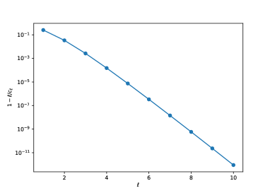
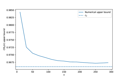
(a) $1-\ell/c_{\ell}$ as a function of $\ell$: the competitive ratio converges exponentially fast to $1$.	(b) Comparison between the upper (obtained by numerical optimization) and lower bound for $\ell=2$.

Figure 1: Numerical evaluation of the competitive ratio.

4 Tightness of the lower bound

We would like to understand how tight the lower bound $\ell/c_{\ell}$ actually is. In this section, we provide numerical results for the computation of $c_{\ell}$, and show that the problem of directly computing $\operatorname{CR}_{\ell}(n)$ is easier than it seems, as it can be reduced from an infinite dimensional optimization problem over the space of measures to a finite dimensional optimization problem over $[0,1]^{2n+2}$. This gives us upper bounds on $\operatorname{CR}_{\ell}$, and we can see that our lower bound is almost optimal.

Let us now consider ways to find good upper bounds on $\operatorname{CR}_{\ell}$. We will transform a continuous distribution $F$ over $[0,1]$ into a discrete one, by using the balayage method from Hill and Kertz (1982, Definition $2.2$)), which basically given an interval transport all the probability mass inside the interval to its extremities so as to preserve expectations. The full description of the method, and the proof of the next proposition can be found in Section 7.13.

Proposition 4.

The value of $\operatorname{CR}_{\ell}$ is attained by discrete distributions with support on $n+1$ points in $[0,1]$.

This result provides a numerical method to find an upper bound on the competitive ratio, by optimizing on all distribution supported on $n+1$ points. This gives an upper bound on $\operatorname{CR}_{\ell}(n)$ (and not the exact value) because we cannot guarantee that our numerical algorithm provides the optimal solution. In Figure 1(b), we compare the resulting numerical upper bound for $\ell=2$ with that of our theoretical lower bound of $\ell_{2}/c_{2}$. We observe that our lower bound is very close to the best upper bound that we managed to find, but there still seems to be a gap. This can be due to two different reasons, either the high-dimensionality of the problem makes it challenging to reach a global optimum, or the constant $2/c_{2}$ is actually not tight. Nevertheless, this gives us a pretty narrow range on the exact worst-case competitive ratio. Because the final gap between the upper and lower bound is so small, we conjecture that it is indeed due to a failed convergence to a global minimum, and we conjecture that $\inf_{n\geq\ell}\operatorname{CR}_{\ell}(n)=\ell/c_{\ell}$.

5 Extension to the selection of $k$ items

Until now we have assumed, that the number of items that can be selected by the decision maker is only $1$. Here, we consider an extension of the problem where the decision maker sequentially selects $k$ items, and where all the items can be selected at most once. This corresponds to the more general setting of Kennedy (1987), which encloses the previous model.

5.1 General algorithm and guarantees

This section focuses on giving guarantees on $\operatorname{CR}_{k,\ell}(n)$ for $k>1$. This time, the algorithm needs to be adaptive not only in $n$ but also in $k$. We define the quantile algorithm Algorithm 2, which takes as an input the known distribution $F$, and for $j\in[k]$, the increasing sequences $0=\vcentcolon\varepsilon^{j}_{j-1}<\varepsilon^{j}_{j}<\dots<\varepsilon^{j}_{n}\vcentcolon=1$. The algorithm is the direct extension of Algorithm 1. The only difference is that, in this new version, the algorithm uses thresholds that depend both on the number of items already observed ($i-1$) and on the number of items we already selected ($j-1$).

Algorithm 2 Quantile algorithm for $(k,\ell)$

Input: Partition $(\epsilon_{i}^{j})_{j-1\leq i\leq n}$ of $[0,1]$ for all $j\in[k]$, distribution $F$ of the $X_{i}$.

$j\leftarrow 1$ // We are currently selecting the $j$th item.

for $i\in[n]$: do

     Draw $q^{j}_{i}$ from $\mathrm{Beta}(\ell,n-\ell)$ truncated between $\epsilon^{j}_{i-1}$ and $\epsilon^{j}_{i}$

     if $X_{i}\geq F^{-1}(1-q^{j}_{i})$ then

         Accept item $i$

         if $j=k$ then

              Stop // because we selected $k$ items

         else

              $j\leftarrow j+1$

         end if

     end if

end for

Similarly to earlier, we define $\alpha^{j}_{i}\vcentcolon=\int_{\varepsilon^{j}_{i-1}}^{\varepsilon^{j}_{i}}\psi_{\ell,n-\ell}(x)dx=\beta_{\ell,n-\ell}(\epsilon_{i}^{j})-\beta_{\ell,n-\ell}(\epsilon_{i-1}^{j})$, and $a_{i}^{j}=\alpha_{i}^{j}\mathbb{E}[(1-q_{i}^{j})]$ where $\mathbb{E}[(1-q_{i}^{j})]$ is the expected probability of not selecting item $i$ when we are observing it and have currently already selected $j-1$ items. Similarly to Proposition 1, we can obtain a guarantee on $\operatorname{ALG}_{k,n}\vcentcolon=\mathbb{E}[\sum_{j\in[k]}X_{\tau_{j}}]$, the performance of Algorithm 2, with respect to $\operatorname{OPT}_{\ell,n}$.

Proposition 5.

We have the inequality

$$\frac{\sum_{j=1}^{k}\min_{i\in\{j,\dots,n\}}\rho_{i}^{j}}{n}\operatorname{OPT}_{\ell,n}\leq\operatorname{ALG}_{k,n}\leq\frac{\sum_{j=1}^{k}\max_{i\in\{j,\dots,n\}}\rho_{i}^{j}}{n}\operatorname{OPT}_{\ell,n},$$ (20)

where

$$\rho_{i}^{j}=\frac{1}{\alpha_{i}^{j}}\sum_{1\leq t_{1}<\dots<t_{j-1}\leq i-1}\left[\prod_{s=1}^{j-1}\left(1-\frac{a_{t_{s}}^{s}}{\alpha_{t_{s}}^{s}}\right)\prod_{r_{1}=1}^{t_{1}-1}\frac{a^{1}_{r_{1}}}{\alpha^{1}_{r_{1}}}\dots\prod_{r_{j}=t_{j-1}+1}^{i-1}\frac{a^{j}_{r_{j}}}{\alpha^{j}_{r_{j}}}\right].$$ (21)

Sketch of proof.

This is similar to Proposition 1, the main difference being that the performance of the algorithm conditionally on the $q_{i}$ being already drawn is more difficult to express. See Section 7.7 for the proof. ∎

Remark that the $\rho_{i}^{j}$ are only defined for $i\geq j$, as time $j$ is the first possible time for the $j$-th item to be selected. If for all $j\in[k]$, we have that the $\rho_{i}^{j}$ are all equal in $i$, meaning that $\rho_{i}^{j}=\rho_{j}^{j}$, then this readily implies from the previous proposition that $\operatorname{ALG}_{k,n}=\frac{\sum_{j\in[k]}\rho_{j}^{j}}{n}\operatorname{OPT}_{\ell,n}$, and that

$$\operatorname{CR}_{k,\ell}(n)\geq\frac{\ell}{k}\frac{\sum_{j\in[k]}\rho_{j}^{j}}{n}\operatorname{OPT}_{\ell,n},$$ (22)

For all $j\in[k]$, we want to find the $\epsilon_{i}^{j}$ that equalizes all the $\rho_{i}^{j}$ across the different $i$. Here, looking at the expression of $\rho_{i}^{j}$, finding any meaningful recurrence relationship might seem hopeless. However, remark that the probability of reaching item $i$ while waiting to select item $j$ only depends on the $\epsilon_{r}^{t}$ for $t\leq j$ and $r\geq t$, and thus so does $\rho_{i}^{j}$. This implies that in order to equalize the $\rho_{i}^{j}$ across $i$, it must be done inductively over $j$: first select the $\epsilon_{i}^{1}$ such that $\rho_{i}^{j}=\rho_{1}^{j}$, then select the $\epsilon_{i}^{2}$ such that $\rho_{i}^{2}=\rho_{2}^{2}$, and so on. We show that, this is equivalent to a system of $k$ difference equations in a non-linear transformation of the $\epsilon_{i}^{j}$.

Lemma 4.

For $b_{i}^{j}=\beta_{\ell,n-\ell}(\epsilon_{i}^{j})$, the condition that for all fixed $j$ the $\rho_{i}^{j}$ are equalized, is equivalent to the following system of difference equations over the $b_{i}^{j}$:

$$\Delta[b_{i}^{j}] =-\frac{\ell}{n}\left(\beta_{\ell+1,n-\ell}\circ\beta_{\ell,n-\ell}^{-1}(b_{i}^{j})-\frac{\rho_{j-1}^{j-1}}{\rho_{j}^{j}}\beta_{\ell+1,n-\ell}\circ\beta_{\ell,n-\ell}^{-1}(b_{i}^{j-1})\right)+b_{j}^{j},\quad j\geq 2 i\geq j$$ for , (23)

$$\Delta[b_{i}^{1}] =-\frac{\ell}{n}\left(\beta_{\ell+1,n-\ell}\circ\beta_{\ell,n-\ell}^{-1}(b_{i}^{1})\right)+b_{1}^{1},\quad i\geq 1$$ for (24)

Sketch of proof.

The most difficult part, is to actually identify the recurrence relationship between the $\alpha_{i}^{j}$ and $a_{i}^{j}$ that the equality of the $\rho_{i}^{j}$ imposes. While it was immediate for $j=1$ as we simply had $\alpha_{i+1}^{1}=a_{i}^{1}$, it is not clear what relationship can be obtained for $j\geq 2$. Fortunately, a simple relation is obtained by incorporating for $j$ the previous constant $\rho_{j-1}^{j-1}$. Indeed, this is equivalent for $j>1$ to $\alpha_{i+1}^{j}=a_{i}^{j}+(\alpha_{i}^{j-1}-a_{i}^{j-1})(\rho_{j-1}^{j-1})/\rho_{j}^{j}$. From there, obtaining the recurrence relation is as before based on the properties of the Beta function. For the proof, see Section 7.8. ∎

We define $\theta_{j,\ell}(n)\vcentcolon=\rho_{j-1}^{j-1}/\rho_{j}^{j}$. From this recurrence relation, we can prove the existence of the solution to the system of boundary discrete value problem by using the exact same continuity argument as in Proposition 2. The proof is however much more technically involved, and requires using several estimates of $b_{j}^{j}$ and $\theta_{j,\ell}(n)$ when $n$ grows large.

Proposition 6.

There exists some $n_{0}\in\mathbb{N}$, such that for $n\geq n_{0}$, there exist $k$ increasing sequences $0=\epsilon_{j-1}^{j}<\epsilon_{j}^{j}<\dots<\epsilon_{n}^{j}=1$ for $j\in[k]$ and $c_{j,\ell}(n)$ such that: for a given $j$ all the $\rho_{i}^{j}$ are equal, $b_{j}^{j}=c_{j,\ell}(n)\cdot n^{-\ell\cdot(((\ell+1)/\ell)^{j}-1)}$ with $c_{j,\ell}(n)$ being bounded between two positive constants independent of $n$.

Sketch of proof.

The quantities $b_{n}^{j}$ are still the composition of continuous functions (yet different functions for each $i\geq j+1$), so the same intermediate value argument can be applied to prove existence, using that if $\theta_{j,\ell}(n)$ is too big or too small compared to some constants, so is $b_{n}^{j}$ compared to $1$. Regarding the exponent in $n$, it can be proved by induction using the relation between $c_{j,\ell}(n)$ and $\theta_{j,\ell}(n)$. The monotonicity comes from the requirement that all the $\rho_{i}^{j}$ are equal and thus must be of the same sign. See section 7.9 for the full proof. ∎

This proposition suggests that the discrete boundary value problem can be approximated in the limit by the continuous boundary value problem in Theorem 3.

The goal is then to find $(c_{1,\ell},\theta_{2,\ell},\dots,\theta_{k,\ell})$ such that this non-linear ODE system admits a solution $b=(b^{1},\dots,b^{k})$ over $[0,1]$, which will be unique. Note that these constants can be found by sequentially solving the $j$-th ODE and finding the $j$-th relevant constant.

Through Proposition 5, solving the discrete boundary value problem for a finite $n$ directly translates to a lower bound on the competitive ratio $\operatorname{CR}_{k,\ell}(n)$. To show that the limiting competitive ratio can also be lower bounded, we must show that the solutions $\theta_{j}(n)$ to the discrete problem converge, which naturally ends up being the solution to the above continuous boundary value problem.

Proposition 7.

Let $c_{1,\ell},\theta_{1},\dots,\theta_{k}$ be the constants such that the boundary value problem in Theorem 3 admits a solution. We have that $\lim_{n\rightarrow\infty}\theta_{j,\ell}(n)=\theta_{j,\ell}$, and $\theta_{j,\ell}\geq 1$. Moreover, this also implies the convergence of $c_{j,\ell}(n)$ toward a constant $c_{j,\ell}$ for all $j\in[k]$, with for the relationship:

$$\theta_{j,\ell}=\frac{(\ell+1)c_{j,\ell}}{\ell(\ell!)^{1/\ell}\cdot c_{j-1,\ell}^{1+1/\ell}}.$$ (25)

Sketch of proof.

The main idea is to couple the convergence of the Euler scheme with the uniform convergence of the drift function, as the difference equations are an Euler scheme using $\beta_{\ell,n-\ell}$ instead of $\gamma_{\ell}$. If the discrete solution converges to the continuous solution, then this implies that $b^{j}(1)=1$. Therefore the limit of $\theta_{j,\ell}(n)$, where we reason with sub-sequences when necessary, must be the unique constant $\theta_{j,\ell}$ such that the boundary value problem admits a solution. However, a key technical difficulty is that the Euler method requires Lipschitzness of the drift function, which is not true for $\gamma_{\ell+1}\circ\gamma_{\ell}^{-1}$ over $[0,1]$. Thus we must use refined arguments proving the convergence on $[0,1-\epsilon]$ to then extend the convergence over $[0,1]$. The full proof can be found in Section 7.10 ∎

We now combine the above results to prove Theorem 3. Letting $\theta_{1,\ell}=1$ for ease of notation, we have that $\rho_{i}^{j}=\rho_{j}^{j}=1/(c_{1,\ell}\cdot\prod_{t\in[k]}\theta_{t,\ell})$, and therefore applying $\liminf$ on the inequality from Proposition 5 and using that the $\theta_{j,\ell}$ converge from Proposition 7,

$$\liminf_{n\rightarrow\infty}\operatorname{CR}_{k,\ell}(n)\geq\liminf_{n\rightarrow\infty}\frac{\sum_{j\in[k]}\rho_{j}^{j}(n)}{n}=\lim_{n\rightarrow\infty}\frac{\ell}{k}\frac{1}{c_{1,\ell}(n)}\sum_{j\in[k]}\frac{1}{\prod\limits_{t\in[j]}\theta_{t,\ell}(n)}=\frac{\ell}{k}\frac{1}{c_{1,\ell}}\sum_{j\in[k]}\frac{1}{\prod\limits_{t\in[j]}\theta_{t,\ell}},$$ (26)

which concludes the proof.

5.2 Numerical results for general setting

Using numerical optimization, we compute the constants $\theta_{j,\ell}$ and provide in Table 2 the numerical value of the asymptotic lower bound on $\operatorname{CR}_{k,\ell}(n)$ from Theorem 3. We also display the solution to the continuous boundary value problem for $k=\ell=5$ in Figure 2.

	1	2	3	4	5
1	0.745	0.966	0.997	0.9998	0.999993
2	0.486	0.829	0.964	0.995	0.9995
3	0.332	0.645	0.864	0.964	0.993
4	0.24997	0.498	0.724	0.885	0.964
5	0.19997	0.3998	0.596	0.772	0.898

Table 2: First digits of $(\ell/k)\sum_{j\in[k]}\prod_{t\in[j]}\theta_{t}^{-1}/c_{1,\ell}$.

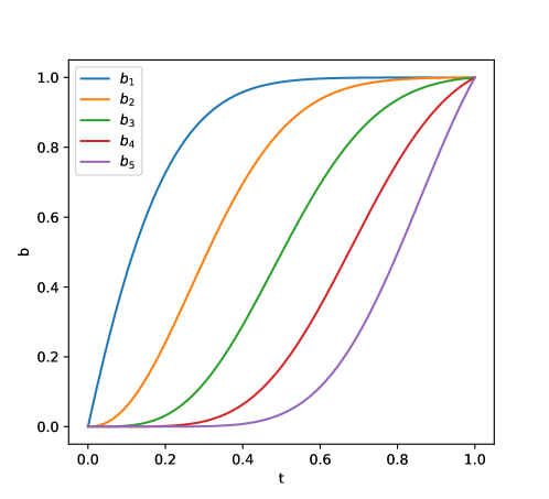
Figure 2: Solution to the continuous boundary value problem for $k=\ell=5$.

For upper bounds on $\operatorname{CR}_{k,\ell}$, we can prove a similar reduction of the infinite dimensional problem to a finite dimensional one, by applying the balayage technique from Hill and Kertz (1982)

Proposition 8.

The value of $\operatorname{CR}_{k,\ell}$ is attained by a discrete distribution with a support of $2+k(k-1)/2+k(n-k)$ points on $[0,1]$.

See section 7.13 for the proof. This proposition is actually stronger than a similar result of Jiang et al. (2022) (Lemma $7.2$), which shows that for the $(k,k)$ case, using an increasingly finer discretization over values to solve the optimization problem $\operatorname{CR}_{k,k}(n)$, yields an increasingly closer solution to the minimum over all possible distributions. Here we have shown that not only can this be extended to any general $(k,\ell)$ setting, but mainly that the minimum distribution must lie in a discretization linear in $n$, and that it is unnecessary to make the discretization any bigger.

6 Static thresholds

We now restrict the competitive ratio analysis to the set of static threshold policies. Similarly to previous works Arnosti and Ma (2021), we allow for random tie breaks when the distributions are discrete. For simplicity, the exposition will use continuous distribution.

In the i.i.d. single item setting, it has been known that the threshold $F^{-1}(1-1/n)$ achieves a competitive ratio of $1-1/e$. A simple alternate proof of this fact was presented in Correa et al. (2019b) using the representation of $\mathbb{E}[\max_{i}X_{i}]$ as the expectation of $nR(Q)$ for $Q$ distributed according to some distribution, and the Jensen inequality. As we have generalized this result and obtained that $\operatorname{OPT}_{\ell,n}$ is equal to $n\mathbb{E}[R(Q)]$ with $Q$ distributed according to $\mathrm{Beta}(\ell,n-\ell)$, we use the same method to prove the following lower bound:

Proposition 9.

The performance of the algorithm that uses static threshold $T=F^{-1}(1-\ell/n)$ is greater than

$$\frac{\sum_{j=1}^{k}\gamma_{j}(\ell)}{k}-\frac{1}{n}\left(1-\gamma_{j}(\ell)-\frac{\ell^{j-1}e^{-\ell}}{(j-1)!}\right)-o\left(\frac{1}{n^{2}}\right).$$ (27)

For the full proof see Section 7.11. Compared to the proof of $1-1/e$ in Correa et al. (2017), multiple additional algebraic manipulations are necessary. This result is actually even more precise, in the sense that the expected reward of the $j$-th item is up to the error term exactly $\gamma_{j}(\ell)/\ell$. One aspect of this result that is remarkable, is that the threshold only depends on $\ell$ and not on $k$. This is quite surprising as this suggests targeting the expected demand of the prophet for the decision-maker to achieve a good competitive ratio.

To obtain an upper bound, we can adapt results from Arnosti and Ma (2021) which deals with $k$ multi-unit static threshold prophet secretary, but it so happens that their worst case instance is i.i.d. We use the following modified example: Let $F^{*}$ be the distribution such that $X=1$ with probability $1-1/n^{2}$, and $X=nW_{k,\ell}$ with probability $1/n^{2}$ where

$$W_{k,\ell}=\frac{\ell^{2}}{k}\frac{\Pr(\mathrm{Poisson}(\ell)<k)}{\Pr(\mathrm{Poisson}(\ell)>k)}.$$ (28)

This example provides an asymptotically tight upper bound:

Proposition 10.

For $(T^{*},p^{*})$ the optimal static threshold and random tie-break under $F^{*}$, we have

$$\lim_{n\rightarrow\infty}\frac{\mathbb{E}_{X\sim F}\left[\frac{1}{k}\sum_{i\in[k]}X_{T^{*}_{i}}\right]}{\mathbb{E}_{X\sim F}\left[\frac{1}{\ell}\sum_{i\in[\ell]}X_{(i)}\right]}=\frac{\sum_{j=1}^{k}\gamma_{j}(\ell)}{k}.$$ (29)

The full proof can be found in Section 7.12. The combination of these two results immediately yields the claimed near tightness $\sum_{j=1}^{k}\gamma_{j}(\ell)/k$ of Theorem 4.

We compute $\sum_{j=1}^{k}\gamma_{j}(\ell)/k$ for different $k$ and $\ell$ and represent them in the left plot of Figure 3. We observe that when either $k$ or $\ell$ or both grow large, the competitive ratio goes towards $\min(\ell/k,1)$. In addition, the convergence to seems to be the slowest for $k=\ell$ and otherwise exponential, away from $k=\ell$, as can be observed on the right plot of Figure 3.

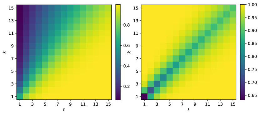
Figure 3: For $k,\ell\in[15]$: on the left $\operatorname{CR}_{k,\ell}^{S}$, on the right $\operatorname{CR}_{k,\ell}^{S}\cdot\min(\ell/k,1)$

This result is intuitive, and we present a simple explanation for $\ell=1$ and $k$ arbitrary. For the single item i.i.d. worst case instance, the first maximum is very far from the second maximum, and thus all other statistics. For this specific distribution, while having a large $k$ allows a greater probability of selecting the actual maximum, all the other selected values will be negligible compared to the maximum. Hence the expected reward of the decision maker will approach $\mathbb{E}[\max_{i}X_{i}]$, and the mean reward $\mathbb{E}[\max_{i}X_{i}]/k$ which leads to a competitive ratio of order $1/k$.

An interesting open question is whether similar guarantees extend to the prophet secretary setting, where distributions are not identical anymore and arrive in random order. In Arnosti and Ma (2021), the $k=\ell$ case is studied, which proves that expected demand policies are not tight for $k\leq 4$, but are tight whenever $k=\ell>4$. The proof of the general $k\neq\ell$ setting presented here relies heavily on the i.i.d. assumption, but it is likely that the values of the competitive ratio remain similar to the i.i.d. setting

7 Detailed proofs

7.1 Proof of Proposition 1

Let $R(q)\vcentcolon=q\mathbb{E}[X\mid X>F^{-1}(1-q)]$ be the expected reward when rejecting values below the $1-q$ quantile of $F$. Through a change of variable, it can be shown that $R(q)=\int_{0}^{q}F^{-1}(\theta)d\theta$.

The first step is to express the performance of $\operatorname{ALG}_{n}$ using the fact that the $q_{i}$ are independently drawn from $\psi_{\ell,n-\ell}$ truncated between $\epsilon_{i-1}$ and $\epsilon_{i}$. This specific step is the same as in Correa et al. (2017). The expected probability of not selecting any item up to $i$ is simply $\mathbb{E}[\prod_{j\in[i]}(1-q_{j})]$, and using the independence of the $q_{i}$ it can be expressed as

$$\mathbb{E}[\prod_{j\in[i]}(1-q_{j})]=\prod_{j\in[i]}\mathbb{E}[(1-q_{j})]=\prod_{j\in[i]}\frac{a_{j}}{\alpha_{j}}.$$

Then, using that $R(q_{i})$ is the expected value of selecting or not item $i$ with threshold $q_{i}$, we have for $\operatorname{ALG}$ the expected performance of the algorithm that

$$\operatorname{ALG} =\sum_{i=1}^{n}\mathbb{E}[R(q_{i})\prod_{j\in[i-1]}(1-q_{j})]$$

$$=\sum_{i=1}^{n}\mathbb{E}[R(q_{i})]\prod_{j\in[i-1]}\frac{a_{j}}{\alpha_{j}}$$

$$=\sum_{i=1}^{n}\int_{\epsilon_{i-1}}^{\epsilon_{i}}R(q_{i})\frac{\psi_{\ell,n-\ell}(q_{i})}{\alpha_{i}}\prod_{j\in[i-1]}\frac{a_{j}}{\alpha_{j}}$$

$$=\sum_{i=1}^{n}\rho_{i}\int_{\epsilon_{i-1}}^{\epsilon_{i}}R(q_{i})\psi_{\ell,n-\ell}(q_{i}),$$

where $\rho_{i}\vcentcolon=\alpha_{i}^{-1}\prod_{j\in[i-1]}a_{j}/\alpha_{j}$.

Hence, we obtain that

$$\operatorname{ALG}_{n} =\sum_{i=1}^{n}\rho_{i}\int_{\epsilon_{i-1}}^{\epsilon_{i}}R(q)\psi_{\ell,n-\ell}(q)dq$$

$$\geq\min_{i\in[n]}\rho_{i}\sum_{i=1}^{n}\int_{\epsilon_{i-1}}^{\epsilon_{i}}R(q)\psi_{\ell,n-\ell}(q)dq=\min_{i\in[n]}\rho_{i}\int_{0}^{1}R(q)\psi_{\ell,n-\ell}(q)dq.$$

We will now show that this last integral is actually equal to $\operatorname{OPT}_{\ell,n}/n$. This was done as a special case in Correa et al. (2017), but for $\ell\geq 2$ this requires the use of the distributions of order statistics.

We recall the distribution of order statistics: the density of $X_{(i)}$ for $i\in[n]$ is

$$\frac{n!}{(n-i)!(i-1)!}f(x)F(x)^{n-i}(1-F(x))^{i-1}.$$

Hence because $\operatorname{OPT}_{\ell,n}=\sum_{i=1}^{\ell}\mathbb{E}[X_{(i)}]$ we can express $\operatorname{OPT}_{\ell,n}$ using those order statistics distributions. Using the change of variable $q=1-F(t)$ and doing integration by parts, we obtain

$$\operatorname{OPT}_{\ell,n} =\sum_{i\in[\ell]}\int_{0}^{\omega}\frac{n!}{(n-i)!(i-1)!}tf(t)F(t)^{n-i}(1-F(t))^{i-1}dt$$

$$=\sum_{i\in[\ell]}\int_{0}^{1}\frac{n!}{(n-i)!(i-1)!}F^{-1}(1-q)(1-q)^{n-i}q^{i-1}dq$$

$$=\sum_{i\in[\ell]}\int_{0}^{1}\frac{n!}{(n-i)!(i-1)!}(1-q)^{n-i-1}q^{i-2}((n-i)q-(i-1)(1-q))\int_{0}^{q}F^{-1}(\theta)d\theta dq$$

$$=\sum_{i\in[\ell]}\int_{0}^{1}\frac{n!}{(n-i)!(i-1)!}(1-q)^{n-i-1}q^{i-2}((n-i)q-(i-1)(1-q))R(q)dq,$$

Exchanging sum and integral, we can observe that the sum is actually telescoping:

$$\sum_{i\in[\ell]}\frac{n!}{(n-i)!(i-1)!}(1-q)^{n-i-1}q^{i-2}((n-i)q-(i-1)(1-q))$$

$$=\sum_{i=1}^{\ell}\frac{n!}{(n-i-1)!(i-1)!}(1-q)^{n-i-1}q^{i-1}-\sum_{i=2}^{\ell}\frac{n!}{(n-i)!(i-2)!}(1-q)^{n-i}q^{i-2}$$

$$=\sum_{i=1}^{\ell}\frac{n!}{(n-i-1)!(i-1)!}(1-q)^{n-i-1}q^{i-1}-\sum_{i=1}^{\ell-1}\frac{n!}{(n-i-1)!(i-1)!}(1-q)^{n-i-1}q^{i-1}$$

$$=\frac{n!}{(n-\ell-1)!(\ell-1)!}(1-q)^{n-\ell-1}q^{\ell-1}$$

$$=n\frac{(n-1)!}{(n-\ell-1)!(\ell-1)!}(1-q)^{n-\ell-1}q^{\ell-1}$$

$$=n\frac{q^{\ell-1}(1-q)^{n-\ell-1}}{B(\ell,n-\ell)}$$

$$=n\psi_{\ell,n-\ell}.$$

Therefore, given this algorithm, we can already deduce that for a given $n\in\mathbb{N}$,

$$\operatorname{CR}_{\ell}(n)\geq\frac{\min_{i\in[n]}\rho_{i}}{n}.$$

7.2 Proof of lemma 1

We first recall a property of $\beta_{\ell,n-\ell}$ which can be obtained by integration by parts.

$$\beta_{\ell+1,n-\ell}(z) =\beta_{\ell,n-\ell}(z)-\frac{z^{\ell}(1-z)^{n-\ell}}{kB(\ell,n-\ell)}$$

$$\beta_{\ell,n-\ell+1}(z) =\beta_{\ell,n-\ell}(z)+\frac{z^{\ell}(1-z)^{n-\ell}}{(n-\ell)B(\ell,n-\ell)}.$$

First we remark that we can express $\alpha_{i}$ as $\beta_{\ell,n-\ell}(\epsilon_{i})-\beta_{\ell,n-\ell}(\epsilon_{i-1})=b_{i}-b_{i-1}$. Similarly for $a_{i}$,

$$a_{i} =\int_{\epsilon_{i-1}}^{\epsilon_{i}}(1-q)\psi_{\ell,n-\ell}(q)dq=\frac{\int_{\epsilon_{i-1}}^{\epsilon_{i}}q^{\ell-1}(1-q)^{n+1-\ell}dq}{B(\ell,n-\ell)}$$

$$=\frac{B(\ell,n+1-\ell)}{B(\ell,n-\ell)}\frac{\int_{\epsilon_{i-1}}^{\epsilon_{i}}q^{\ell-1}(1-q)^{n+1-\ell}dq}{B(\ell,n+1-\ell)}$$

$$=\frac{\frac{\Gamma(\ell)\Gamma(n+1-\ell)}{\Gamma(n+1)}}{\frac{\Gamma(\ell)\Gamma(n-\ell)}{\Gamma(n)}}(\beta_{\ell,n+1-\ell}(\epsilon_{i})-\beta_{\ell,n+1-\ell}(\epsilon_{i-1})$$

$$=\frac{n-\ell}{n}(\beta_{\ell,n+1-\ell}(\epsilon_{i})-\beta_{\ell,n+1-\ell}(\epsilon_{i-1}).$$

The quantities $\rho_{i}$ always satisfy a simple recurrence relation, namely that $\rho_{i+1}=a_{i}\rho_{i}/\alpha_{i+1}$. So imposing the equality of the $\rho_{i}$ is equivalent to the relation $\alpha_{i+1}=a_{i}$. Now, using this relationship:

$$\alpha_{i+2} =a_{i+1}$$

$$\Leftrightarrow\ \beta_{\ell,n-\ell}(\epsilon_{i+2})-\beta_{\ell,n-\ell}(\epsilon_{i+1})=\frac{n-\ell}{n}(\beta_{\ell,n+1-\ell}(\epsilon_{i+1})-\beta_{\ell,n+1-\ell}(\epsilon_{i}))$$

$$\Leftrightarrow\ b_{i+2}-b_{i+1}=\frac{n-\ell}{n}\Big{(}\beta_{\ell,n-\ell}(\epsilon_{i+1})-\beta_{\ell,n-\ell}(\epsilon_{i})$$

$$+\frac{\epsilon_{i+1}^{\ell}(1-\epsilon_{i+1})^{n-\ell}}{(n-\ell)B(\ell,n-\ell)}-\frac{\epsilon_{i}^{\ell}(1-\epsilon_{i})^{n-\ell}}{(n-\ell)B(\ell,n-\ell)}\Big{)}$$

$$\Leftrightarrow\ \Delta[b_{i+1}]=\Delta[b_{i}]-\Big{(}\frac{\ell}{n}\beta_{\ell,n-\ell}(\epsilon_{i+1})-\frac{\epsilon_{i+1}^{\ell}(1-\epsilon_{i+1})^{n-\ell}}{nB(\ell,n-\ell)}$$

$$-\frac{\ell}{n}\beta_{\ell,n-\ell}(\epsilon_{i+1})+\frac{\epsilon_{i+1}^{\ell}(1-\epsilon_{i+1})^{n-\ell}}{nB(\ell,n-\ell)}\Big{)}$$

$$\Leftrightarrow\ \Delta^{2}[b_{i}]=-\frac{\ell}{n}\Delta\left[\beta_{\ell,n-\ell}(\epsilon_{i})-\frac{\epsilon_{i}^{\ell}(1-\epsilon_{i})^{n-\ell}}{\ell B(\ell,n-\ell)}\right]$$

$$\Leftrightarrow\ \Delta^{2}[b_{i}]=-\frac{\ell}{n}\Delta[\beta_{\ell+1,n-\ell}(\epsilon_{i})]$$

$$\Leftrightarrow\ \Delta^{2}[b_{i}]=\frac{\Delta[-\ell\beta_{\ell+1,n-\ell}(\beta_{\ell,n-\ell}^{-1}(b_{i}))]}{n}.$$

By summing those equations, we can hence obtain an explicit recurrence relationship on $b_{i}$. Indeed, for $i\geq 2$:

$$\sum_{j=0}^{i-2}\Delta^{2}[b_{j}] =\sum_{j=0}^{i-2}\frac{\Delta[-\ell\beta_{\ell+1,n-\ell}(\beta_{\ell,n-\ell}^{-1}(b_{j}))]}{n}$$

$$\Leftrightarrow\ (b_{i}-b_{i-1})-(b_{1}-b_{0})=\frac{-\ell(\beta_{\ell+1,n-\ell}(\beta^{-1}_{\ell,n-\ell}(b_{i}))-\beta^{-1}_{\ell,n-\ell}(0))}{n}$$

$$\Leftrightarrow\ b_{i}=b_{i-1}-\frac{\ell}{n}\beta_{\ell+1,n-\ell}\circ\beta^{-1}_{\ell,n-\ell}(b_{i})+b_{1}.$$

7.3 Proof of Proposition 2

Because $\beta_{\ell,n-\ell}(0)=0$ and $\beta_{\ell,n-\ell}(1)=1$, the problem of finding an increasing partition of $\epsilon_{i}$ which satisfies $\rho_{i+1}=\rho_{i}$ with $\epsilon_{0}=0$ and $\epsilon_{n}=1$ is equivalent to finding a partition of the $b_{i}$ which satisfies the recurrence relation in Equation 13, which is a specific instance of a discrete boundary value problem. We will now prove that there exists a $b_{1}$ such that $b_{n}=1$, such that $b_{i+1}\geq b_{i}$ and it solves the discrete boundary value problem.

Let us take care of the monotonicity first. Suppose that the correct $b_{1}$ is strictly smaller than $\ell/n$. Then because $\rho_{1}=1/\alpha_{1}=1/b_{1}>n/\ell$, we have that the competitive ratio for a given $n$ is greater than $\ell\rho_{1}/n>1$ which is impossible as it must be smaller than $1$ (take a constant distribution). Hence, $b_{1}\geq\ell/n$. Note that for $b_{1}\geq\ell/n$ and because $\beta_{\ell+1,n-\ell}(x)\leq 1$, we have that

$$b_{i+1}-b_{i}=-\frac{\ell}{n}\beta_{\ell+1,n-\ell}\circ\beta^{-1}_{\ell,n-\ell}(b_{i})+b_{1}\geq-\frac{\ell}{n}+\frac{\ell}{n}\geq 0.$$

This implies that any $b_{1}\geq\ell/n$ yield an increasing sequence of $b_{i}$, hence an increasing sequence of $\epsilon_{i}$. So if there exists a valid $b_{1}$, the sequence associated must be increasing.

Now for the existence, remark first that $b_{n}$ can be expressed at $n-1$ composition of the recurrence relation, which is continuous, so $b_{n}$ is a continuous function of $b_{1}$. For $b_{1}=0$, the recurrence relation implies that $b_{n}=0$. For $b_{1}\geq(\ell+1)/n$, bounding the difference $b_{i+1}-b_{i}$ as above, yields $\Delta[b_{i}]\geq 1/n$, meaning that $b_{n}\geq 1$. By intermediate value theorem over $b_{1}$, and using that any $b_{1}$ smaller than $\ell/n$ does not work, we have that there exists a $b_{1}\in[\ell/n,(\ell+1)/n]$ which solves the boundary value problem.

7.4 Proof of Lemma 2

We recall that the distribution function of the ${\ell}$-th order statistic for a random variable with distribution $F$ is simply $\beta_{n+1-{\ell},{\ell}}\circ F$. If we show that $\beta_{n+1-{\ell},{\ell}}\circ F\geq\beta_{2n+1-{\ell},{\ell}}\circ\sqrt{F}$, then $Y_{({\ell})}$ stochastically dominates $X_{({\ell})}$, which implies the desired result of $\mathbb{E}[Y_{({\ell})}]\geq\mathbb{E}[X_{({\ell})}]$ (this is immediate from writing the expectation of a positive random variable as $\int_{0}^{\infty}1-F$).

Let us look at the function $h(x)\vcentcolon=\beta_{n+1-{\ell},{\ell}}(x)-\beta_{2n+1-{\ell},{\ell}}(\sqrt{x})$ for $x\in[0,1]$. Clearly if we show that this function is non-negative over $[0,1]$, then so is $h\circ F$ over $\mathbb{R}^{+}$. Let us consider the derivative of $h$ using the density of the beta distribution:

$$\frac{dh(x)}{dx}=\frac{x^{n-{\ell}}(1-x)^{{\ell}-1}}{B(n+1-{\ell},{\ell})}-\frac{\sqrt{x}^{2n-{\ell}-1}(1-\sqrt{x})^{{\ell}-1}}{2B(2n+1-{\ell},{\ell})}.$$

For simplicity, let $\sqrt{x}=y\in[0,1]$ then we can rewrite the above derivative as

$$\frac{dh(x)}{dx} =\frac{y^{2n-2{\ell}}(1-y^{2})^{{\ell}-1}}{B(n+1-{\ell},{\ell})}-\frac{y^{2n-{\ell}-1}(1-y)^{{\ell}-1}}{2B(2n+1-{\ell},{\ell})}$$

$$=\frac{y^{2n-2{\ell}}(1-y)^{{\ell}-1}(1+y)^{{\ell}-1}}{B(n+1-{\ell},{\ell})}-\frac{y^{2n-{\ell}-1}(1-y)^{{\ell}-1}}{2B(2n+1-{\ell},{\ell})}$$

$$=\frac{y^{2n-{\ell}-1}(1-y)^{{\ell}-1}}{B(n+1-{\ell},n)}\left(\frac{(1+y)^{{\ell}-1}}{y^{{\ell}-1}}-\frac{B(n+1-{\ell},{\ell})}{2B(2n+1-{\ell},{\ell})}\right).$$

Hence over $[0,1]$, $h^{\prime}(x)\geq 0$ is equivalent to

$$\left(1+\frac{1}{y}\right)^{{\ell}-1}\geq\frac{B(n+1-{\ell},{\ell})}{2B(2n+1-{\ell},{\ell})}.$$

The function on the left is equal to $\infty$ at $y=0$, and is decreasing in $y$: this implies that the derivative is positive until some $y_{0}=\sqrt{x_{0}}$, and then possibly negative. If a function is increasing then decreasing over an interval, then its minimum is at the endpoints of the interval. And we have that $h(0)=h(1)=0$, so $h(x)\geq\min_{x^{\prime}\in[0,1]}h(x^{\prime})=0$, which concludes the proof.

7.5 Proof of Lemma 3

We first recall a limiting relationship between incomplete Gamma and Beta functions. We have for $X_{n}\sim\mathrm{Beta}(\ell,n)$ that the random variable $Y_{n}=nX_{n}$ converges in law to $\mathrm{Gamma}(\ell)$ as $n$ goes to $\infty$.

In particular this means that

$$\lim_{n\rightarrow\infty}\beta_{\ell,n-\ell}\left(\frac{z}{n}\right)=\lim_{n\rightarrow\infty}\Pr(X_{n}\leq\frac{z}{n})=\lim_{n\rightarrow\infty}\Pr(nX_{n}\leq z)=\gamma_{\ell}(x),$$

where the last equality stems from the equivalence between limit in distribution and point-wise limit of the distribution function (we also indirectly use that $\ell X_{n}$ goes to $0$ for $k$ fixed).

Let us show the point-wise convergence. The inverse of $\beta_{{\ell},n-{\ell}}(\cdot/n)$ is simply $n\beta_{{\ell},n-{\ell}}^{-1}$. Because $\beta_{{\ell},n-{\ell}}$ is continuous, the point-wise limit of the inverse is the inverse of the point-wise limit. Hence $\lim_{n\rightarrow\infty}\beta_{{\ell},n-{\ell}}^{-1}=\gamma_{\ell}^{-1}$. Rewriting the main function as $-{\ell}\beta_{\ell+1,n-{\ell}}\circ\text{id}/n\circ n\cdot\text{id}\circ\beta_{{\ell},n-{\ell}}^{-1}$ we have by composition that this converges to $-{\ell}\gamma_{\ell+1}\circ\beta_{{\ell}}^{-1}$.

Now for the uniform convergence. First, note that because of the expansion formula, we have that $\beta_{{\ell},n+1-{\ell}}\geq\beta_{{\ell},n-{\ell}}$ which means that $\beta_{{\ell},n+1-{\ell}}^{-1}\leq\beta_{{\ell},n-{\ell}}^{-1}$ (interpolating over $n$ if necessary) so $\beta_{{\ell},n-{\ell}}^{-1}$ decreasing in $n$, and $\beta_{\ell+1,n+1-{\ell}}\geq\beta_{{\ell},n-{\ell}}$ so $\beta_{\ell+1,n+1-{\ell}}^{-1}$ increasing in $n$. This implies that $\beta_{\ell+1,n-{\ell}}\circ\beta_{{\ell},n-{\ell}}^{-1}$ is decreasing in $n$, and finally $-{\ell}\beta_{\ell+1,n-{\ell}}\circ\beta_{{\ell},n-{\ell}}^{-1}$ is increasing in $n$. Because this function is continuous and takes values in $[0,1]$ which is compact, we can apply Dini’s Theorem which guarantees uniform convergence.

Remark.

Note that we can similarly express this ODE using $\nu=\gamma_{\ell}^{-1}(b)\in[0,\infty)$ to avoid the use of an inverse functions:

$$\frac{d^{2}}{dt^{2}}(\gamma_{\ell}(\nu))=-{\ell}\frac{d}{dt}(\gamma_{\ell+1}(\nu)).$$

It is not immediately clear what $\nu$ represents compared to the $\epsilon_{i}$. Indeed, we had that $\beta_{{\ell},n-{\ell}}^{-1}(b_{i})=\epsilon_{i}$, but $\nu$ cannot directly translate into $\epsilon_{i}$ as $\nu\in[0,\infty)$ whereas $\epsilon_{i}\in[0,1]$. Actually, we can definite $\nu_{i}=n\epsilon_{i}$, which implies that

$$\Delta^{2}[\beta_{{\ell},n-{\ell}}(\frac{\nu_{i}}{n})]=\frac{\Delta[-{\ell}\beta_{\ell+1,n}(\frac{\nu_{i}}{n})]}{n},$$

which converges using the exact same limiting argument for the pointwise limit as above to the second order ODE which $\nu(t)$ obeys. So $\nu$ is the limit of $n\epsilon_{i}$. This is to put in perspective to the limit in Correa et al. (2017) where the ODE concerned used $y_{i}=(1-\epsilon_{i})^{n-1}$.

7.6 Proof of Proposition 3

Let $\xi_{{\ell},n}(x)=-{\ell}\beta_{\ell+1,n-{\ell}}\circ\beta_{{\ell},n-{\ell}}^{-1}(x)$ and $\xi_{\ell}(x)=-\ell\gamma_{\ell+1}\circ\gamma_{\ell}^{-1}(x)$. First

$$b_{i+1}-b_{i}=\frac{\xi_{{\ell}}(b_{i})+c_{1,\ell}}{n}+\frac{c_{1,\ell}(n)-c_{1,\ell}}{n}+\frac{\xi_{{\ell},n}(b_{i})-\xi_{\ell}(b_{i})}{n}$$

Now let us divide both side by $\xi_{{\ell}}(b_{i})+c_{1,\ell}$ (which is strictly positive as $c_{1,\ell}$ must be strictly greater than ${\ell}$)

$$\frac{c_{1,\ell}(n)-c_{1,\ell}}{n(\xi_{\ell}(b_{i})+c_{1,\ell})}=-\frac{1}{n}+\frac{b_{i+1}-b_{i}}{\xi_{\ell}(b_{i})+c_{1,\ell}}-\frac{\xi_{{\ell},n}(b_{i})-\xi_{\ell}(b_{i})}{n(\xi_{\ell}(b_{i})+c_{1,\ell})}$$

Remark also that for $x\in[0,1]$, $x\mapsto-{\ell}x+\zeta_{\ell}(x)+c_{1,\ell}$ is bounded between $c_{1,\ell}-{\ell}>0$ and $c_{1,\ell}$, therefore,

$$\left|\sum_{i=0}^{n-1}\frac{c_{1,\ell}(n)-c_{1,\ell}}{n(\xi_{\ell}(b_{i})+c_{1,\ell})}\right|\geq\delta|c_{1,\ell}(n)-c_{1,\ell}|,\quad\delta>0.$$

Now using the previous equation,

$$\left|\sum_{i=0}^{n-1}\frac{c_{1,\ell}(n)-c_{1,\ell}}{n(\xi_{\ell}(b_{i})+c_{1,\ell})}\right| \leq\left|-1+\sum_{i=0}^{n-1}\frac{b_{i+1}-b_{i}}{\xi_{\ell}(b_{i})+c_{1,\ell}}\right|+\frac{1}{n(c_{1,\ell}-{\ell})}\sum_{i=0}^{n-1}|\xi_{{\ell},n}(b_{i})-\xi_{\ell}(b_{i})|$$

$$\leq\left|-1+\sum_{i=0}^{n-1}\frac{b_{i+1}-b_{i}}{\xi_{\ell}(b_{i})+c_{1,\ell}}\right|+\frac{1}{(c_{1,\ell}-{\ell})}\|\xi_{{\ell},n}-\xi_{\ell}\|_{\infty}.$$

The last term goes to $0$ by uniform convergence, and the first one by Riemann sum and the integral equation condition, as due to $c_{1,\ell}(n)$ being bounded independently of $n$ we have $b_{i+1}-b_{i}=O(1/n)$.

All in all $\lim_{n\rightarrow\infty}c_{1,\ell}(n)=c_{1,\ell}$.

7.7 Proof of Proposition 5

First let us consider the performance of the algorithm, conditionally on the $q_{i}^{j}$ being already drawn. Basically, if while waiting to select the $j$-th item the algorithm arrives at step $i$, then the expected reward received taking into account the probability of actually selecting the item is $R(q_{i}^{j})$. However, the probability of arriving at step $i$ while waiting for item $j$ is more complicated to express. Indeed, first the $j-1$ must be selected before time $i$, and then no item must be selected until $i$ while waiting for $j$. Hence the expected reward at step $i$, when selecting the $j$-the item, can be expressed as

$$\mathbb{E}[R(q^{j}_{i})]\sum_{t_{j-1}=j-1}^{i-1}\sum_{t_{j-2}=j-2}^{t_{j-1}-1}\dots\sum_{t_{1}=1}^{t_{2}-1}\left[\prod_{s=1}^{j-1}\left(1-\frac{a_{t_{s}}^{s}}{\alpha_{t_{s}}^{s}}\right)\prod_{r_{1}=1}^{t_{1}-1}\frac{a^{1}_{r_{1}}}{\alpha^{1}_{r_{1}}}\dots\prod_{r_{j}=t_{j-1}+1}^{i-1}\frac{a^{j}_{r_{j}}}{\alpha^{j}_{r_{j}}}\right],$$

where the $t_{m}$ correspond to the time when item $m$ is selected, and the sums consider all possible times of selection. While this equation seems complicated, it is merely due to the fact that the thresholds depend on $i$ and $j$, and all possible sequences of selection must be considered.

The proposition can then be easily obtained by re-using the fact proved in Proposition 1 that $\operatorname{OPT}_{\ell,n}=\mathbb{E}_{q\sim\psi_{\ell,n-\ell}}[R(q)]$ and that for any $j\in[k]$, the $(\epsilon_{i}^{j})_{i\in\{j-1,\dots,n\}}$ are constructed to form a partition of $[0,1]$.

7.8 Proof of Lemma 4

Let us write down a recursion formula in $i$ on $\rho_{i}^{j}$ that might depend on previous values of $j$. We have already dealt with the case $j=1$ when only one item could be selected by the decision maker. As such, we will assume that $j>1$. Due to $\alpha_{i+1}^{j}\rho_{i+1}^{j}$ being equal to the probability of reaching time $i+1$ with exactly $j-1$ items already selected, denoting $t_{s}$ the time when item $s$ is selected, we have

$$\alpha_{i+1}^{j}\rho_{i+1}^{j} =\sum_{t_{j-1}=j-1}^{i}\sum_{t_{j-2}=j-2}^{t_{j-1}-1}\dots\sum_{t_{1}=1}^{t_{2}-1}\Pr(\text{Selecting item $s$ at time $t_{s}$ for $s\in[j-1]$})$$

$$=\sum_{t_{j-1}=j-1}^{i}\sum_{t_{j-2}=j-2}^{t_{j-1}-1}\dots\sum_{t_{1}=1}^{t_{2}-1}\left[\prod_{s=1}^{j-1}\left(1-\frac{a^{s}_{t_{s}}}{\alpha^{s}_{t_{s}}}\right)\prod_{r_{1}=1}^{t_{1}-1}\frac{a^{1}_{r_{1}}}{\alpha^{1}_{r_{1}}}\dots\prod_{r_{j}=t_{j-1}+1}^{i}\frac{a^{j}_{r_{j}}}{\alpha^{j}_{r_{j}}}\right]$$

$$=\sum_{t_{j-1}=j-1}^{i-1}\sum_{t_{j-2}=j-2}^{t_{j-1}-1}\dots\sum_{t_{1}=1}^{t_{2}-1}\left[\prod_{s=1}^{j-1}\left(1-\frac{a^{s}_{t_{s}}}{\alpha^{s}_{t_{s}}}\right)\prod_{r_{1}=1}^{t_{1}-1}\frac{a^{1}_{r_{1}}}{\alpha^{1}_{r_{1}}}\dots\prod_{r_{j}=t_{j-1}+1}^{i}\frac{a^{j}_{r_{j}}}{\alpha^{j}_{r_{j}}}\right]$$

$$+\sum_{t_{j-2}=j-2}^{i-1}\dots\sum_{t_{1}=1}^{t_{2}-1}\left[\prod_{s=1}^{j-1}\left(1-\frac{a^{s}_{t_{s}}}{\alpha^{s}_{t_{s}}}\right)\prod_{r_{1}=1}^{t_{1}-1}\frac{a^{1}_{r_{1}}}{\alpha^{1}_{r_{1}}}\dots\prod_{r_{j}=i+1}^{i}\frac{a^{j}_{r_{j}}}{\alpha^{j}_{r_{j}}}\right]$$

$$=\frac{a^{j}_{i}}{\alpha_{i}^{j}}\sum_{t_{j-1}=j-1}^{i-1}\sum_{t_{j-2}=j-2}^{t_{j-1}-1}\dots\sum_{t_{1}=1}^{t_{2}-1}\left[\prod_{s=1}^{j-1}\left(1-\frac{a^{s}_{t_{s}}}{\alpha^{s}_{t_{s}}}\right)\prod_{r_{1}=1}^{t_{1}-1}\frac{a^{1}_{r_{1}}}{\alpha^{1}_{r_{1}}}\dots\prod_{r_{j}=t_{j-1}+1}^{i-1}\frac{a^{j}_{r_{j}}}{\alpha^{j}_{r_{j}}}\right]$$

$$+\left(1-\frac{a^{j-1}_{i}}{\alpha^{j-1}_{i}}\right)\sum_{t_{j-2}=j-2}^{i-1}\dots\sum_{t_{1}=1}^{t_{2}-1}\left[\prod_{s=1}^{j-2}\left(1-\frac{a^{s}_{t_{s}}}{\alpha^{s}_{t_{s}}}\right)\prod_{r_{1}=1}^{t_{1}-1}\frac{a^{1}_{r_{1}}}{\alpha^{1}_{r_{1}}}\dots\prod_{r_{j-1}=t_{j-2}+1}^{i-1}\frac{a^{j}_{r_{j-1}}}{\alpha^{j}_{r_{j-1}}}\right]$$

$$=\alpha_{i}^{j}\rho_{i}^{j}+(\alpha_{i}^{j-1}-a_{i}^{j-1})\rho_{i}^{j-1}.$$

Notably, if we let the $\epsilon_{i}^{j}$ be such that $\rho_{i}^{j}=\rho_{j}^{j}$ for all $i\in\{j,\dots,n\}$ (starting from $j=1$, and sequentially imposing the boundary values), then dividing both sides by $\rho_{j}^{j}$ we obtain

$$\alpha_{i+1}^{j}=a_{i}^{j}+(\alpha_{i}^{j-1}-a_{i}^{j-1})\frac{\rho_{j-1}^{j-1}}{\rho_{j}^{j}}.$$

this overall yields a grid of recurrence equations for $j>1$ and $i\geq j$. Now let us translate this recurrence relationship into one over $b_{i}^{j}$. Let us assume that $\rho_{i+1}^{j-1}=\rho_{i}^{j}$ and see what this implies for $j$, with $j=1$ being already treated in Equation 13.

Following the same computations done in Lemma 1, we have that $\alpha_{i+2}^{j}-a_{i+1}^{j}=\text{cst}$ is equivalent to $\Delta^{2}[b_{i}^{j}]=\frac{\Delta[-\ell\beta_{\ell+1,n-\ell}\circ\beta_{\ell,n-\ell}^{-1}(b_{i}^{j})]}{n}+\text{cst}$. Then, using that $\alpha_{i+1}^{j-1}-a_{i+1}^{j-1}=\alpha_{i+2}^{j-1}-\alpha_{i+2}^{j-1}+\alpha_{i+1}^{j-1}-a_{i+1}^{j-1}=-(\alpha_{i+2}^{j-1}-\alpha_{i+1}^{j-1})$, we obtain

$$\Delta^{2}[b_{i}^{j}] =\frac{\Delta[-\ell\beta_{\ell+1,n-\ell}\circ\beta_{\ell,n-\ell}^{-1}(b_{i}^{j})]}{n}-\frac{\rho_{j-1}^{j-1}}{\rho_{j}^{j}}\Delta^{2}[b_{i}^{j-1}]$$

$$=\frac{\Delta[\frac{\rho_{j-1}^{j-1}}{\rho_{j}^{j}}\ell\beta_{\ell+1,n-\ell}\circ\beta_{\ell,n-\ell}^{-1}(b_{i}^{j-1})-\ell\beta_{\ell+1,n-\ell}\circ\beta_{\ell,n-\ell}^{-1}(b_{i}^{j})]}{n}.$$

Now summing these equations yields the desired result.

7.9 Proof of Proposition 6

We outline here the main steps for the proof: First, it must be that $b_{j}^{j}=o(1)$, as otherwise, because we add $b_{j}^{j}$ for $n-j$ steps, $b_{n}^{j}=\Omega(n)>1$. Then we show that if $\theta_{j,\ell}(n)\vcentcolon=\rho_{j-1}^{j-1}/\rho_{j}^{j}$ is larger than some positive constant (independent of $n$) then $b_{n}^{j}>1$, and if it is smaller than some positive constant then $b_{n}^{j}<1$. By the intermediate value theorem, as $b^{j}_{n}$ is a continuous function of $b_{j}^{j}$, there must be a value $b_{j}^{j}$ such that $b^{j}_{n}=1$, which proves the existence. Moreover, by giving an asymptotic expression of $\theta_{j,\ell}(n)$ in terms of $b_{j}^{j}$ and $b_{j-1}^{j-1}$, and because $\theta_{j,\ell}(n)$ must remain bounded between two positive constants, we can inductively give an asymptotic expression of $b_{j}^{j}$ in terms of $n$ as $b_{j}^{j}=\Theta(n^{r_{j,\ell}})$ with $r_{j,\ell}=\ell\cdot(1-(\frac{\ell+1}{\ell})^{j})$. Then we show that the $b_{i}^{j}$ remain between $0$ and $1$, allowing us to map back the $b_{i}^{j}$ solution to a solution on the $\epsilon_{i}^{j}$. Finally, by evaluating the sign of $\rho_{i}^{j}$ if any $\epsilon_{i+1}^{j}$ were to be smaller than an $\epsilon_{i}^{j}$, we can obtain a contradiction, thus implying that the $\epsilon_{i}^{j}$ must be increasing in $i$, and so does the $b_{i}^{j}$. All of the above will be proven inductively for each $j$, so the aforementioned properties will be assumed true for $j-1$, and the initialization to $j=1$ already corresponds to Proposition 2.

Upper bound on $\theta_{j,\ell}(n)$. Let us inductively show that $\theta_{j,\ell}(n)$ is bounded where we temporarily re-define (only in this proof!) $\theta_{1,\ell}(n)\vcentcolon=(\ell+1)/\ell$. Using the recurrence relation from Lemma 4, we have that

$$\Delta[b_{i}^{j}] \geq\frac{1}{n}\left(\theta_{j,\ell}(n)\ell\beta_{\ell+1}\circ\beta_{\ell}^{-1}(b_{i}^{j-1})-\ell\right)$$

$$\implies b_{n}^{j}+o(1)=b_{n}^{j}-b_{j}^{j}=\frac{1}{n}\sum_{i=j}^{n-1} \Delta[b_{i}^{j}] \geq\ell\left(\theta_{j,\ell}(n)\left(\frac{1}{n}\sum_{i=j}^{n-1}\beta_{\ell+1,n-\ell}\circ\beta_{\ell,n-\ell}^{-1}(b_{i}^{j-1})\right)-1\right)+o(1)$$

$$\geq\ell\left(\theta_{j,\ell}(n)\left(\frac{1}{n}\sum_{i=j}^{n-1}\gamma_{\ell+1}\circ\gamma_{\ell}^{-1}(b_{i}^{j-1})\right)-1\right)+o(\theta_{j,\ell}(n)),$$

where the last equality is due to the uniform convergence in Lemma 3. We now need to lower bound the above sum. Due to the induction hypothesis, we have that $b_{n}^{j-1}=1$, $b_{j}^{j}=o(1/n)$ for $j>1$ and thus $\Delta[b_{i}^{j-1}]\leq\theta_{j-1}\ell/n+o(1/n)$ (this is why we define $\theta_{1,\ell}(n)=(\ell+1)/\ell$ to make sure that this expression remains true for $j=1$ as $\Delta[b_{i}^{1}]\leq(\ell+1)/n$). Therefore it takes some time to go from any value $y\in(0,1)$ to $1=b_{n}^{j}$. More specifically, if we denote $t$ the first time where $b_{t}^{j-1}\geq y$ we obtain an inequality on $t$:

$$1=b_{t}^{j-1}+\sum_{i=t}^{n-1}\Delta[b_{i}^{j-1}] \leq y+\frac{1}{n}\theta_{j-1}\ell+\frac{n-t-1}{n}\theta_{j-1}\ell+o(1)$$

$$\implies n-t\geq\frac{1-y}{\theta_{j-1}\ell}+o(1).$$

Due to the monotonicity of $b_{i}^{j-1}$ in $i$, for any $i\geq t$, $b_{i}^{j-1}\geq y$. We can now lower bound the sum:

$$b_{n}^{j}\geq\ell\left(\theta_{j,\ell}(n)\frac{(1-y)\gamma_{\ell+1}\circ\gamma_{\ell}^{-1}(y)}{\ell\theta_{j-1}}-1\right)+o(\theta_{j-1}).$$ (30)

We could get tighter bounds on $\theta_{j,\ell}(n)$ if we maximize this inequality in $y$, but let us simply take $y=1/2$, which numerically is not so bad for low values of $\ell$ and looks to be the maximum for large values of $\ell$ anyway. All in all, for $b_{n}^{j}$ to remain below $1$, it must be that

$$\theta_{j,\ell}(n)\leq\frac{2(\ell+1)}{\gamma_{\ell+1}\circ\gamma_{\ell}^{-1}(1/2)}\theta_{j-1}+o(1).$$

Iterating this inequality in $j$ with $\theta_{1,\ell}(n)$ bounded shows that all the $\theta_{j,\ell}(n)$ indeed remain bounded independently of $n$, as we can always find a constant large enough to bound the $o(1)$.

Size estimate of $b_{j}^{j}$. Before showing that $\theta_{j,\ell}(n)$ is bounded below by some positive constant, we will first show that $b_{j}^{j}$ must be very small in front of $1/n$ due to the previous upper bound on $\theta_{j,\ell}(n)$. Let us express $\rho_{j}^{j}$ in terms of $\rho_{j-1}^{j-1}$:

$$\rho_{j}^{j} =\frac{1}{\alpha_{j}^{j}}\prod_{r\in[j-1]}\left(1-\frac{a_{r}^{r}}{\alpha_{r}^{r}}\right)=\frac{1}{\alpha_{j}^{j}}\left(1-\frac{a^{j-1}_{j-1}}{\alpha_{j-1}^{j-1}}\right)\alpha_{j-1}^{j-1}\rho_{j-1}^{j-1}$$

$$=\frac{1}{\alpha_{j}^{j}}\left(\alpha_{j-1}^{j-1}-a^{j-1}_{j-1}\right)\rho_{j-1}^{j-1}$$

$$=\frac{\ell\beta_{\ell+1,n-\ell}\circ\beta_{\ell,n-\ell}^{-1}(b_{j-1}^{j-1})}{nb_{j}^{j}}\rho_{j-1}^{j-1},$$

where the last equality can be obtained following the same computations done in Section 7.2. This implies that $b_{j}^{j}=O((\ell\beta_{\ell+1,n-\ell}\circ\beta_{\ell,n-\ell}(b_{j-1}^{j-1}))/n)$.

The expansion of $\beta_{\ell,n-\ell}^{-1}(x)$ around $0$ is $(\ell\cdot xB(\ell,n-\ell))^{1/\ell}+o(x^{1/\ell})=(\ell\cdot x)^{1/\ell}/n+o(1)$. Using the combinatorial formula for $\beta_{\ell+1,n-\ell}$, we have

$$\ell\beta_{\ell+1,n-\ell}\circ\beta_{\ell,n-\ell}(b_{j}^{j}) =\ell\sum_{t=\ell+1}^{n}\binom{n}{t}\beta_{\ell,n-\ell}^{-1}(b_{j}^{j})^{t}\cdot(1-\beta_{\ell,n-\ell}^{-1}(b_{j}^{j}))^{n-t}$$

$$=\ell\frac{n^{\ell+1}}{(\ell+1)!}\frac{(\ell!\cdot b_{j}^{j})^{1+1/\ell}}{n^{\ell+1}}+o((b_{j}^{j})^{1+1/\ell})$$

$$=\frac{\ell}{\ell+1}(\ell!)^{1/\ell}(b_{j}^{j})^{1+1/\ell}+o((b_{j}^{j})^{1+1/\ell}).$$ (31)

The second equality is because $(1-\beta_{\ell,n-\ell}^{-1})^{n-t}\rightarrow_{n\rightarrow\infty}1$ as long as $b_{j}^{j}=o(1)$, and because

$$\binom{n}{t+1}\beta_{\ell,n-\ell}^{-1}(b_{j}^{j})^{t+1}/(\binom{n}{t}\beta_{\ell,n-\ell}^{-1}(b_{j}^{j})^{t})=O((b_{j}^{j})^{\ell})=o(1),$$

so the first term of the sum dominates the other ones. Hence, using the growth rate induction hypothesis $b_{j-1}^{j-1}=\Theta(n^{r_{j-1},\ell})$, we can upper bound $b_{j-1}^{j-1}$ by $O(n^{(1+1/\ell)r_{j-1,\ell}-1})$. We now solve the recurrence $r_{j,\ell}=((\ell+1)/\ell)r_{j-1,\ell}-1$ which will allow us to conclude that $b_{j}^{j}\leq O(n^{r_{j,\ell}})$. The first term and the fixed point of this recurrence are respectively $r_{1,\ell}=-1$ and $\ell$, a classic exercise shows that $r_{j,\ell}=-((\ell+1)/\ell)^{j-1}(1+\ell)+\ell=-\ell(((\ell+1)/\ell)^{j}-1)$. Moreover, for $j>1$, $r_{j,\ell}<-1$, meaning that $b_{j}^{j}=o(n^{-1})$.

Lower bound on $\theta_{j,\ell}(n)$. We can now proceed to lower bound $\theta_{j,\ell}(n)$. For $\Delta[b_{i}^{j}]$ to be big enough and for $b_{n}^{j}$ to reach $1$, $\theta_{j,\ell}(n)$ must be large enough. Indeed

$$\Delta[b_{i}^{j}]\leq\frac{\theta_{j,\ell}(n)\ell}{n}+b_{j}^{j}=\frac{\theta_{j,\ell}(n)\ell}{n}+o(\frac{1}{n}),$$

using the previous upper bound on $b_{j}^{j}$ and that $0\leq\beta_{\ell+1,n-\ell}\leq 1$. Therefore $b_{n}^{j}\leq\theta_{j,\ell}(n)\ell+o(1)$, which implies that if $\theta_{j,\ell}(n)$ is strictly smaller than $1/\ell+o(1)$, then $b_{n}^{j}$ is smaller than $1$. We can then apply the intermediate value theorem to the function $b_{n}^{j}(b_{j}^{j})$ to obtain the existence, and for the value $b_{j}^{j}$ which satisfies the boundary value condition, it must be that $\theta_{j,\ell}(n)\geq 1/\ell+o(1)$. Using once again the expression of $\theta_{j,\ell}(n)$ and induction hypothesis on $b_{j-1}^{j-1}$, we can conclude that $b_{j}^{j}=\Omega(n^{r_{j,\ell}})$ and therefore that $b_{j}^{j}=c_{j,\ell}n^{r_{j,\ell}}$ with $c_{j,\ell}\in[1/\ell,(2(\ell+1)/(\gamma_{\ell+1}\circ\gamma_{\ell}^{-1}(1/2)))^{j-1}(\ell+1)/\ell]$. The actual constants could be tightened, and this would immediately yield a lower bound on the competitive ratio, akin to using the bound $c_{1,\ell}\leq\ell+1$ to prove that $\operatorname{CR}_{1,\ell}\geq\ell/(\ell+1)$.

Mapping $b_{i}^{j}$ back to $\epsilon_{i}^{j}$. To ensure that the solution to the discrete boundary value problem in $b_{i}^{j}$ translates into a solution to the discrete boundary value problem in $\epsilon_{i}^{j}$, we must ensure that the $b_{i}^{j}$ remain in $[0,1]$ for $\beta_{\ell,n-\ell}^{-1}(b_{i}^{j})$ to be well defined. For $b_{i}^{j}\leq 1$, one way to see this is to define a continuous extension of $\beta_{\ell+1,n-\ell}\circ\beta_{\ell,n-\ell}(x)$ by $1$ for any $x>1$, and by $0$ whenever $x<0$. This ensures that if for some $i$, $b_{i}^{j}>1$ then it remains strictly greater than $1$. Indeed for $t_{1}$ the first time it crosses $1$ the difference $\Delta[b_{t_{1}}^{j}]$ must be positive, and for any $t>t_{1}$ $\Delta[b_{t}^{j}]\geq\Delta[b_{t_{1}}^{j}]\geq 0$ due to the monotonicity of $b_{i}^{j-1}$ by the induction hypothesis and due to the continuous extension which remains fixed at $1$. This entails that $b_{n}^{j}>1$. This is a contradiction with $b_{n}^{j}=1$.

Now let us show that the $b_{i}^{j}$ that solves the boundary value problem always remain positive. The main idea is that, due to the size of the $b_{j}^{j}$, the sequence must be increasing at the beginning and hence positive, and after some time because the difference between two consecutive terms is bounded and the $b_{i}^{j-1}$ are increasing, it cannot go below a certain positive threshold without going back up. First, when $b_{i}^{j}=o(1)$, we can always approximate $\ell\beta_{\ell+1,n-\ell}\circ\beta_{\ell,n-\ell}(b_{i}^{j})=L(b_{i}^{j})^{1+1/\ell}+o((b_{i}^{j})^{1+1/\ell})$, where $L=\frac{\ell}{\ell+1}(\ell!)^{1/\ell}$. From a high level, what this means is that whenever $x$ is small when we compare $x$ and $\beta_{\ell+1,n-\ell}\circ\beta_{\ell,n-\ell}^{-1}(x)\approx L\cdot x\cdot x^{1/\ell}$ the first will dominate the second. So, for any $i\leq n/\log(n)$, $\Delta[b_{i}^{1}]=c_{1,\ell}/n+o(1/n)$, and $b_{i}^{1}=c_{1,\ell}(i/n)+o(i/n)$. From there we can verify by induction that for $i\leq n/\log(n)$, $b_{i}^{j}=\kappa_{j}\cdot(n/i)^{r_{j,\ell}}+o((n/i)^{r_{j,\ell}})$ with $\kappa_{j}$ bounded between two positive constant independent of $n$, and $r_{j,\ell}=-\ell(((\ell+1)/\ell)^{j}-1)$. We can start by upper bounding $\Delta[b_{i}^{j}]$ using $i\leq n/\log(n)$ by

$$\Delta[b_{i}^{j}] \leq\theta_{j,\ell}(n)L\frac{1}{n}(b_{i}^{j-1})^{1/\ell+1}+c_{j,\ell}(n)n^{r_{j,\ell}}$$

$$\leq\theta_{j,\ell}(n)L\kappa_{j-1}^{1+1/\ell}\frac{1}{n}\left(\frac{n}{i}\right)^{(1+1/\ell)\cdot r_{j-1,\ell}}+c_{j,\ell}(n)n^{r_{j,\ell}}$$

$$\leq\kappa_{j}\frac{\log(n)^{(1+1/\ell)\cdot r_{j,\ell}}}{n}+o(\frac{\log(n)^{(1+1/\ell)\cdot r_{j,\ell}}}{n}),$$

with $\kappa_{j}=\theta_{j,\ell}(n)L\kappa_{j}^{1+1/\ell}+c_{j,\ell}(n)$. This implies that for $i\leq n/\log(n)$:

$$b_{i}^{j}\leq\kappa_{j}(i\log(n)^{(1+1/\ell)\cdot r_{j,\ell}})/n+o((i\log(n)^{(1+1/\ell)\cdot r_{j,\ell}})/n)\leq\kappa_{j}\log(n)^{r_{j,\ell}}+o(\log(n)^{r_{j,\ell}}).$$

Therefore $b_{i}^{j}$ is negligible in front of $b_{i}^{j-1}$, so we can redo the same computations by replacing above the inequality by an equality as $\beta_{\ell+1,n-\ell}\circ\beta_{\ell,n-\ell}^{-1}(b_{i}^{j})$ is negligible in front of $\beta_{\ell+1,n-\ell}\circ\beta_{\ell,n-\ell}^{-1}(b_{i}^{j-1})$. This also implies that $\Delta[b_{i}^{j}]\geq 0$ as the only negative term is negligible. We obtain $b_{i}^{j}=\kappa_{j}\cdot(n/i)^{r_{j,\ell}}+o((n/i)^{r_{j,\ell}})$. Now for $i=\lfloor\log(n)/n\rfloor$, we have that $b_{i}^{j}=\kappa_{j}\log(n)^{r_{j,\ell}}+o(\log(n)^{r_{j,\ell}})$, which is strictly greater than $\ell/n$, an upper bound on the minimum value of $\Delta[b_{i}^{j}]$ derived from Lemma 4. Because $\Delta[b_{i}^{j}]\geq 0$ for any $i\leq n/log(n)$ and $b_{i}^{j-1}$ is non decreasing, for any $t$ such that $b_{i}^{j}\leq b_{n/\log(n)}$ we have that $\Delta[b_{t}^{j}]\geq\Delta[b_{n/\log(n)}^{j}]\geq 0$. Thus the sequence $b_{i}^{j}$ cannot keep on decreasing when going below $b_{n/\log(n)}^{j}$, and $b_{n/\log(n)}^{j}-\ell/n>0$ which overall yields the non-negativity of the $b_{i}^{j}$.

Monotonicity of the $b_{i}^{j}$. It remains to show the monotonicity. The quantity $\rho_{i}^{j}$, while it stems from a probabilistic event that had assumed that the $\epsilon_{i}^{j}$ were increasing, can be defined for any $\epsilon_{i}^{j}$ using integrals with no further requirements on the $\epsilon_{i}^{j}$. For now, we have shown that there exists $\epsilon_{i}^{j}$ such that all the $\rho_{i}^{j}$ are equal, $\epsilon_{j-1}^{j}=0$ and $\epsilon_{n}^{j}=1$. First, the sign of $\alpha_{i}^{j}\rho_{i}^{j}$ is always positive. Indeed, $\alpha_{i}^{j}$ and $a_{i}^{j}$ are of the same sign, positive if $\epsilon_{i}^{j}\geq\epsilon_{i-1}^{j}$, and negative otherwise. In both cases, the ratio is positive and smaller than $1$, which also implies the positivity of $1-a_{i}^{j}/\alpha_{i}^{j}$. As a sum of products of positive terms, $\alpha_{i}^{j}\rho_{i}^{j}$ is always positive. Because all the $\rho_{i}^{j}$ are equal, they have the same sign, so either all the $\rho_{i}^{j}$ and $\alpha_{i}^{j}$ are positive, or they are all negative. Because $\epsilon_{j-1}^{j}=0$ and $\epsilon_{n}^{j}=1$, there must be some $t\geq j$ such that $\epsilon_{t}^{j}\geq\epsilon_{t-1}^{j}$, implying that $\alpha_{t}^{j}$ is positive. Therefore all the $\alpha_{i}^{j}=\beta_{\ell,n-\ell}(\epsilon_{i}^{j})-\beta_{\ell,n-\ell}(\epsilon_{i-1}^{j})$ are positive, which means that the $\epsilon_{i}^{j}$ are non-decreasing. Finally, because $\epsilon_{j-1}^{n}=0\neq 1=\epsilon_{n}^{j}$, then at least one of the $\rho_{i}^{j}$ is finite, which by equality of the $\rho_{i}^{j}$ means that all them must be finite, and so all the $\epsilon_{i}^{j}$ are distinct. Hence the $\epsilon_{i}^{j}$ are non-decreasing and distinct, so are increasing.

7.10 Proof of Proposition 7

Due to the uniform convergence in Lemma 3, it seems intuitive that we do have the convergence from the discrete boundary value problem to the continuous one. However, there are many technical difficulties that make proving this convergence especially challenging, in particular the fact that the limit function $\gamma_{\ell+1}\circ\gamma_{\ell}^{-1}$ is not Lipschitz over $[0,1]$ having an infinite derivative at $1$. The convergence of $c_{1,\ell}(n)$ is already proven in Proposition 3, so it remains to prove the convergence of $\theta_{j,\ell}(n)$ towards $\theta_{j,\ell}$ (the solution to the continuous boundary value problem).

Let $\xi_{{\ell},n}(x)=-{\ell}\beta_{\ell+1,n-{\ell}}\circ\beta_{{\ell},n-{\ell}}^{-1}(x)$ and $\xi_{\ell}(x)=-\ell\gamma_{\ell+1}\circ\gamma_{\ell}^{-1}(x)$. First due to the boundedness of the sequence $\theta_{j,\ell}(n)$, by the Bolzano-Weierstrass theorem there is at least one subsequence with an accumulation point $\theta$, and we will work with such a subsequence.

Existence of solution to ODE. We now consider the ODE $y^{\prime}(t)=\xi_{\ell}(y)-\theta\xi_{\ell}(b^{j-1}(t))$ with initial condition $y(0)=0$. as $\xi_{\ell}$ and $\xi_{\ell}(b^{j-1}(t))$ are continuous, there exists a solution $b^{j}$ over $[0,1]$. We also have that

$$\xi_{\ell}^{\prime}(x)=-\ell\cdot(\gamma_{\ell}^{-1})^{\prime}(x)\cdot(\gamma_{\ell+1})^{\prime}(\gamma_{\ell}^{-1}(x))=-\ell\cdot\frac{\gamma_{\ell+1}^{\prime}\circ\gamma_{\ell}^{-1}(x)}{\gamma_{\ell}^{\prime}\circ\gamma_{\ell}^{-1}(x)}=-\gamma_{\ell}^{-1}(x),$$

so as long as $x<1$ then $\xi_{\ell}^{\prime}$ is bounded and $\xi_{\ell}$ Lipschitz over this interval. This means that as long as $b^{j}$ is strictly smaller than $1$, then by the Cauchy Lipschitz theorem the solution must be unique. The case when $\max_{[0,1]}b_{j}<1$ is easier to treat, so we focus on when $\max_{[0,1]}b_{j}\geq 1$. Because $\xi_{\ell}$ is bounded, $b^{j}$ itself is Lipschitz over $[0,1]$, so denoting $t_{1}$ the first time $b^{j}=1$ the solution is unique over $[0,t_{1}]$ due to the Lipschitzness of $b^{j}$. Note that over $(t_{1},1]$ there can be potentially multiple solutions satisfying the initial condition $b^{j}(0)=0$.

We now wish to prove the convergence of $b_{\lfloor tn\rfloor}^{j}$ towards $b^{j}(t)$ for any $t\in[0,t_{1}]$. We will prove it first on $[0,t_{1}-\epsilon]$ for any $\epsilon>0$. The main idea is that $b_{i}^{j}$ is almost an Euler discretization of the continuous solution, and the same ideas used in the convergence of the Euler method can be modified to take into account that the discretization uses $\xi_{\ell,n}$ and not $\xi_{\ell}$.

$b_{\lfloor tn\rfloor}$ and $b(t)$ are different from $1$. Let $t\in[0,t_{1}-\epsilon]$, in which case $b_{j}(t)<1$ by continuity as $t<t_{1}$ and $t_{1}$ is the first time for which $b^{j}(t)=1$. Similarly, we now show that for $n$ large enough, $b_{\lfloor tn\rfloor}\leq 1-c$ for some $c>0$. The quantity $b_{\lfloor tn\rfloor}$ is bounded between $(0,1)$ so has a non-empty set of accumulation points. For $n$ large enough, the distance between $b_{\lfloor tn\rfloor}$ and the set of accumulation points will go to $0$, if not we can look at the sub-sequence of points which do not converge to an accumulation point and apply Bolzano-Weierstrass again to exhibit a new accumulation point towards which at least some of the points converge, showing a contradiction. Therefore, if all the accumulation points are strictly smaller than $1$, then there exists some constant $c$ such that for $n$ large enough $b_{\lfloor tn\rfloor}\leq 1-c$. All the accumulation points must be smaller than $1$ as the $b_{i}^{j}$ are smaller than $1$. Suppose that $1$ belongs to the set of accumulation points. Because $b_{n}^{j}=1$, this means that $b_{n}^{j}-b_{\lfloor tn\rfloor}^{j}=n^{-1}\sum_{i=\lfloor tn\rfloor}^{n}\Delta[b_{i}^{j}]\rightarrow 0$. So, due to the convergence of $b^{j-1}_{i}$ by the induction hypothesis, for any $t^{\prime}\geq\lfloor t\rfloor$ we have $b_{\lfloor t^{\prime}n\rfloor}^{j}\rightarrow 1$, and $n\Delta[b_{\lfloor t^{\prime}n\rfloor}^{j}]\rightarrow\theta f(b^{j-1}(t^{\prime}))-\ell$. Using that $\xi_{\ell,n}$ converges uniformly towards $\xi_{\ell}$, the Riemann sum approximation tells us that $n^{-1}\sum_{i=\lfloor t^{\prime}n\rfloor}^{n}\Delta[b_{i}^{j}]=\int_{t^{\prime}}^{1}\theta\xi_{\ell}(b^{j-1}(u))du-\ell=0$. This equation is valid for any $t^{\prime}>t$, which is not possible as $b^{j-1}$ is increasing and therefore the integral value must be different. Overall, we have proven that the $b_{\lfloor tn\rfloor}^{j}$ must remain far from $1$ as long as $t<1$.

Convergence by Euler’s method. Instead of working with the discrete sequence $b_{i}^{j}$, we work with the affine by parts function $b_{(n)}^{j}$ which takes value $b_{i}^{j}$ at times $i/n$ and each of those values are interpolated through linear segments. We will prove the uniform convergence of this affine by part function to the continuous limit. One way to prove this could be to use the Arzela-Ascoli theorem, as we have now a sequence of functions with approximately the same Lipschitz constant, and are thus equicontinuous. Instead we will apply Euler’s method. Let $\varphi(y,t)=\xi_{\ell}(y)-\theta\xi_{\ell}(b^{j-1}(t))$ and $\varphi_{n}(y,t)=\xi_{\ell,n}(y)-\theta_{j,\ell}(n)\xi_{\ell,n}(b^{j-1}_{(n)}(t))$. The function $\varphi_{n}$ converges uniformly to $\varphi$ due to Lemma 3, that $\theta_{j,\ell}(n)$ converges to some $\theta$ for the subsequence considered, and $b^{j-1}_{(n)}$ converges uniformly to its limit solution. Let $t_{i}=i/n$, and $\delta_{i}=b^{j}(t_{i})-b^{j}_{i}$ be the global truncation error up to time $t_{i}$ (the notation is omitted but $b^{j}_{i}$ depends on $n$). We only consider time $t_{i}$ with $t_{i}\leq t_{1}-\epsilon$, so that $\varphi(y,t)$ is $B$-Lipschitz in $y$ for $B>0$ and $b^{j}(t)^{\prime\prime}=(b^{j})^{\prime}(t)\xi_{\ell}^{\prime}(b^{j}(t))-\theta\cdot(b^{j-1})^{\prime}(t)\xi_{\ell}^{\prime}(b^{j-1}(t))$ is also bounded by some $A>0$ due to the boundedness of $(b^{j-1})^{\prime}$ and $(b^{j})^{\prime}$. Looking at the global truncation error, denoting by $\omega_{n}=\|\varphi_{n}-\varphi\|_{\infty}$, we have

$$|\delta_{i+1}|=|b^{j}(t_{i+1})-b_{i+1}^{j}=b^{j}(t_{i+1})-b_{i}^{j}-\frac{\varphi_{n}(b^{j}_{i},t_{i})}{n}|$$

$$=|b^{j}(t_{i+1})-b_{i}^{j}-\frac{\varphi(b^{j}_{i},t_{i})}{n}+\frac{\varphi(b^{j}_{i},t_{i})-\varphi_{n}(b^{j}_{i},t_{i})}{n}|$$

$$=|b^{j}(t_{i})-b_{i}^{j}+\frac{\varphi(b^{j}(t_{i}),t_{i})-\varphi(b^{j}_{i},t_{i})}{n}+(b^{j}(t_{i+1})-b^{j}(t_{i})-\frac{1}{n}\varphi(b^{j}(t_{i}),t_{i}))+\frac{\varphi(b^{j}_{i},t_{i})-\varphi_{n}(b^{j}_{i},t_{i})}{n}|$$

$$\leq|\delta_{i}|+\frac{1}{n}B|\delta_{i}|+\frac{1}{2}A\frac{1}{n^{2}}+\frac{\omega_{n}}{n}\leq(1+\frac{B}{n})\delta_{i}+\frac{\omega^{\prime}_{n}}{n},$$

where $\omega^{\prime}(n)=\max(A/(2n),\omega_{n})$ which goes to zero as both $A/n$ and $\omega_{n}$ do. Using that $\delta_{0}=0$, we can apply this inequality iteratively leading to

$$\delta_{i}\leq\sum_{j=1}^{i-1}\left(1+\frac{B}{n}\right)^{j}\frac{\omega^{\prime}_{n}}{n}=\frac{\omega^{\prime}_{n}}{n}\frac{(1+B/n)^{i}-1}{1+B/n-1}\leq\omega^{\prime}_{n}\exp((t_{1}-\epsilon)B)\xrightarrow[n\longrightarrow\infty]{}0.$$

Because $t_{i+1}-t_{i}\rightarrow 0$ and by Lipschitzness of $b^{j}_{(n)}$ we have the convergence towards $b^{j}$ for any $t\in[0,t_{1}-\epsilon]$. Finally

$$|b^{j}(t_{1})-b^{j}_{(n)}(t_{1})| \leq|b^{j}(t_{1})-b^{j}(t_{1}-\epsilon)|+|b^{j}(t_{1}-\epsilon)-b^{j}_{(n)}(t_{1}-\epsilon)|+|b^{j}_{(n)}(t_{1}-\epsilon)-b^{j}_{(n)}(t_{1})|$$

$$\leq M\epsilon+\delta_{\lfloor(t_{1}-\epsilon)n\rfloor}(\epsilon)+M\epsilon,$$

with $M$ a common upper bound on $\varphi_{n}$ and $\varphi$ for $n$ large enough. We can take the limit of this inequality over $n$ for any fixed $n$, and then take the limit over $\epsilon$. This implies that $\lim_{n\rightarrow\infty}b^{j}_{(n)}(t_{1})=b^{j}(t_{1})=1$, which is impossible unless $t_{1}=1$ as we have already proven that this limit is different from $1$ as long as $t<1$. This implies that $\theta$ is a solution to the continuous boundary value problem. Yet, there is a unique solution to the continuous boundary value problem, as $b^{j}(1,\theta)$ is increasing in $\theta$. As a consequence, there can only be one accumulation point for $\theta$, implying that $\theta_{j,\ell}(n)$ does converge to the solution of the continuous boundary value problem in Theorem 3.

To finish, $b^{j}$ is non-decreasing as $\Delta[b_{i}^{j}]\geq 0$ and it must remain so in the limit, and because $b^{j-1}$ is strictly increasing (the initialization for this property is that $b^{1}$ is strictly increasing as $c_{1,\ell}>1$), then so is $b^{j}$. Additionally the convergence of $\theta_{j,\ell}(n)$ implies the convergence of $c_{j,\ell}(n)$, and the relation between these two quantities is immediate from taking the limit in Equation 31. The monotonicity of $b^{j}$ immediately implies that $\theta_{j,\ell}\geq 1$, as $(b^{j})^{\prime}(1)=\theta_{j,\ell}\cdot\ell-\ell=\ell(\theta_{j,\ell}-1)\geq 0$.

7.11 Proof of Proposition 9

The proof consists of two steps, using Jensen’s inequality on the reward of the single threshold algorithm similarly done in Correa et al. (2019b) to prove in a simple way the $1-1/e$ performance of $F^{-1}(1-1/n)$ in the i.i.d. single item setting, and algebraic manipulations as well as inequalities to obtain the desired lower bound.

We can start by noting that the expression of the online algorithm when only a single threshold is used is much simpler. Let $q\in[0,1]$ be the quantile corresponding to the selected threshold, e.g. $T=F^{-1}(1-q)$. The expected reward given by the $j$-th item at time $i$ is simply $R(q)$ times the probability of having selected exactly $j-1$ item up to time $i-1$, which corresponds to a random variable distributed according to $\mathrm{Binomial}(i-1,q)$ to be equal to $j-1$. The total expected reward obtained through the $j$-th item is thus

$$\sum_{i=j}^{n}R(q)\binom{i-1}{j-1}q^{j-1}(1-q)^{i-j}.$$

Moreover, we know through the proof of Proposition 1 that for $Q$ distributed according to $\mathrm{Beta}(\ell,n-\ell)$, $\operatorname{OPT}_{\ell,n}=n\mathbb{E}[R(Q)]$. The expectation of $Q$ is $\mathbb{E}[Q]=\ell/n$, and using the concavity of $R$ we obtain

$$\operatorname{OPT}_{\ell,n}=n\mathbb{E}[R(Q)]\leq nR\left(\frac{\ell}{n}\right).$$ (32)

Due to this inequality, we set the deterministic quantile to be $q=\ell/n$, which immediately implies that

$$\sum_{i=j}^{n}R(q)\binom{i-1}{j-1}q^{j-1}(1-q)^{i-j}\geq\left(\sum_{i=j}^{n}\frac{1}{n}\binom{i-1}{j-1}\left(\frac{\ell}{n}\right)^{j-1}\left(1-\frac{\ell}{n}\right)^{i-j}\right)\operatorname{OPT}_{\ell,n}.$$

To obtain a lower bound on this competitive ratio, it remains to lower bound this sum, which we will denote by $S_{j,\ell,n}$.

$$S_{j,\ell,n}=\sum_{i=0}^{n-j}\frac{1}{n}\binom{i+j-1}{j-1}\left(\frac{\ell}{n}\right)^{j-1}\left(1-\frac{\ell}{n}\right)^{i}=\frac{\ell^{j-1}}{n^{j}(j-1)!}\sum_{i=0}^{n-j}\frac{(i+j-1)!}{i!}\left(1-\frac{\ell}{n}\right)^{i}.$$

We recognize that $\sum_{i=0}^{n-j}(i+j-1)\times\dots\times(i+1)(1-\ell/n)^{i}$ is the $j-1$-th derivative of the geometric sum $\sum_{i=0}^{n-1}(1-\ell/n)^{i}=(1-(1-\ell/n)^{n})/(1-(1-\ell/n))$. the $t$-th derivative of $1/(1-x)$ is $t!/(1-x)^{t+1}$ and the $t$-th derivative of $1-x^{n}$ for $t\geq 1$ is $-n!/(n-t)!x^{n-t}\mathbb{1}[t\leq n]$. Using Leibniz rule for derivation,

$$\frac{d^{j-1}}{dx}\frac{1-x^{n}}{1-x} =\sum_{t=0}^{j-1}\binom{t-1}{t}\frac{d^{j-1-t}}{dx}\left(1-x^{n}\right)\frac{d^{t}}{dx}\left(\frac{1}{1-x}\right)$$

$$=(j-1)!\frac{1-x^{n}}{(1-x)^{j}}-\sum_{t=0}^{j-2}\binom{j-1}{t}\cdot\frac{t!}{(1-x)^{t+1}}\cdot\frac{n!}{(n+1+t-j)!}x^{n+1+t-j}$$

$$=(j-1)!\frac{1}{(1-x)^{j}}-\sum_{t=0}^{j-1}\binom{j-1}{t}\cdot\frac{t!}{(1-x)^{t+1}}\cdot\frac{n!}{(n+1+t-j)!}x^{n+1+t-j}$$

For $x=(1-\ell/n)\leq 1$, $x^{n+1+t-j}=(1-\ell/n)^{n+1+t-j}\leq\exp(-\ell)(1-\ell/n)^{1+t-j}$, $(1-x)^{t+1}=(\ell/n)^{t+1}$, and $n!/(n+1+t-j)!\leq n^{j-t-1}$. Therefore

$$S_{j,\ell,n} \geq\frac{\ell^{j-1}}{n^{j}(j-1)!}\left[(j-1)!\frac{1}{(\ell/n)^{j}}-\sum_{t=0}^{j-1}\frac{(j-1)!}{t!(j-1-t)!}\cdot\frac{t!}{(\ell/n)^{t+1}}\cdot n^{j-t-1}\exp(-\ell)(1-\frac{\ell}{n})^{1+t-j}\right]$$

$$=\frac{1}{\ell}\left(1-e^{-\ell}\sum_{t=0}^{j-1}\frac{(\ell/(1-\ell/n))^{j-1-t}}{(j-1-t)!}\right)$$

$$=\frac{1}{\ell}\left(1-e^{-\ell}\sum_{t=0}^{j-1}\frac{(\ell/(1-\ell/n))^{t}}{t!}\right)$$

$$=\frac{1}{\ell}\left(1-e^{\ell^{2}/(n-\ell)}+e^{\ell^{2}/(n-\ell)}-e^{-\ell}\cdot e^{\ell/(1-\ell/n)}\cdot e^{-\ell/(1-n/\ell)}\sum_{t=0}^{j-1}\frac{(\ell/(1-\ell/n))^{t}}{t!}\right)$$

$$=\frac{\gamma_{j}(\ell/(1-\ell/n))e^{\ell^{2}/(n-\ell)}+(1-e^{\ell^{2}/(n-\ell)})}{\ell}\geq\frac{\gamma_{j}(\ell)}{\ell}-\frac{1}{n}\left(\ell-\gamma_{j}(\ell)\cdot\ell-\frac{\ell^{j}e^{-\ell}}{(j-1)!}\right)-o\left(\frac{1}{n^{2}}\right),$$

where we used Taylor approximations to get estimates of $\gamma_{j}(\ell/(1-\ell/n))$, and $e^{\ell^{2}/(n-\ell)}$. Summing the contribution of every item $j\in[k]$, we immediately obtain the desired lower bound

$$\operatorname{CR}^{S}_{k,\ell}(n)\geq\frac{\sum_{j=1}^{k}\gamma_{\ell}(j)}{k}-\frac{1}{n}\left(1-\gamma_{j}(\ell)-\frac{\ell^{j-1}e^{-\ell}}{(j-1)!}\right)-o\left(\frac{1}{n^{2}}\right).$$

7.12 Proof of Proposition 10

Once the worst case instance from Arnosti and Ma (2021) is correctly modified, their proof almost entirely follows through. First of all, they show that for any quantity $W$ independent of $n$, the prophet’s expected reward is at least

$$\ell+W-\frac{1+W}{n+1},$$

and the decision maker’s expected reward is at mots

$$\mathbb{E}[\min(\mathrm{Poisson}(nq),k)]\left(1+\frac{W}{nq}\right)+2kWn^{-2/3}+2kn^{-1/3},$$

with $q$ the probability of accepting any item which is a function of the random tie-break probability. They further show that the derivative of $\mathbb{E}[\min(\mathrm{Poisson}(nq),k)]\left(1+W/nq\right)$ in $\lambda=nq$ is equal to

$$\frac{d}{d\lambda}\mathbb{E}[\min(\mathrm{Poisson}(\lambda),k)]\left(1+\frac{W}{\lambda}\right)=\Pr(\mathrm{Poisson}(\lambda)<k)\left(1-W\frac{k}{\lambda^{2}}\frac{\Pr(\mathrm{Poisson}(\lambda)>k)}{\Pr(\mathrm{Poisson}(\lambda)<k)}\right).$$

To have a simple expression of the competitive ratio, we pick $W=W_{k,\ell}$ such that the above derivative cancels at exactly $\lambda=\ell$. Hence

$$\frac{d}{d\lambda}\mathbb{E}[\min(\mathrm{Poisson}(\lambda),k)]\left(1+\frac{W_{k,\ell}}{\lambda}\right)=\Pr(\mathrm{Poisson}(\lambda)<k)\left(1-\frac{\ell^{2}}{\lambda^{2}}\frac{\Pr(\mathrm{Poisson}(\ell)<k)}{\Pr(\mathrm{Poisson}(\ell)>k)}\frac{\Pr(\mathrm{Poisson}(\lambda)>k)}{\Pr(\mathrm{Poisson}(\lambda)<k)}\right)$$

It remains to show that this critical point corresponds to a maximum. The computations will be almost identical to Arnosti and Ma (2021).

For $\lambda<\ell$ we have

$$\frac{\ell^{2}}{\lambda^{2}}\frac{\Pr(\mathrm{Poisson}(\ell)<k)}{\Pr(\mathrm{Poisson}(\ell)>k)}\frac{\Pr(\mathrm{Poisson}(\lambda)>k)}{\Pr(\mathrm{Poisson}(\lambda)<k)} =\frac{\sum_{j>k}\lambda^{j-2}/j!}{\sum_{j>k}\ell^{j-2}/j!}\cdot\frac{\sum_{j<k}\ell^{j}/j!}{\sum_{j<k}\lambda^{j}/j!}$$

$$<\left(\frac{\lambda}{\ell}\right)^{k-1}\frac{\sum_{j<k}\ell^{j}/j!}{\sum_{j<k}\lambda^{j}/j!}$$

$$=\frac{\sum_{j<k}(\frac{\lambda}{\ell})^{k-1-j}\lambda^{j}/j!}{\sum_{j<k}\lambda^{j}/j!}\leq 1.$$

The same can be done for $\lambda>\ell$, which shows that $nq=\ell$ indeed yields the optimal static rule with tie-break for $F^{*}$.

In the limit as $n\rightarrow\infty$, this implies that

$$\operatorname{CR}_{k,\ell}^{S}\leq\frac{\ell}{k}\cdot\frac{\mathbb{E}[\min(\mathrm{Poisson}(\ell),k)]\left(1+\frac{W_{k,\ell}}{\ell}\right)}{\ell+W_{k,\ell}}=\frac{\mathbb{E}[\min(\mathrm{Poisson}(\ell),k)]}{k}.$$

This last quantity can then be related to $\gamma_{j}(\ell)$, as

$$\mathbb{E}[\min(\mathrm{Poisson}(\ell),k)]=\sum_{j=0}^{k-1}\Pr(\mathrm{Poisson}(\ell)>j) =k-\sum_{j=0}^{k-1}\Pr(\mathrm{Poisson}(\ell)\leq j)$$

$$=\sum_{j=0}^{k-1}\left(1-\sum_{i=0}^{j}\frac{\ell^{i}}{i!}e^{-\ell}\right)$$

$$=\sum_{j=0}^{k-1}\gamma_{j+1}(\ell)$$

$$=\sum_{j=1}^{k}\gamma_{j}(\ell).$$

7.13 Proof on finite dimension reduction

In this section, we take care of proving the reduction procedure, for the general $(k,\ell)$ setting, from a general distribution $F$ to a discrete distribution in $[0,1]$, with a smaller competitive ratio $\operatorname{CR}_{k,\ell}(n)$. This immediately implies the result of Proposition 4 for $(1,\ell)$, and of Proposition 8 for general $(k,\ell)$.

Let us first define the technique of balayage.

Definition 1.

For a random variable $X$ and constants $0\leq a<b<\infty$ we denote by $X_{a:b}$ the random variable which takes the same value as $X$ when $X\not\in[a,b]$, takes value $a$ with probability $p_{a}=\mathbb{E}[(b-X)\mathbb{1}[X\in[a,b]]]/(b-a)$ and takes value $b$ with probability $p_{b}=\mathbb{E}[(X-a)\mathbb{1}[X\in[a,b]]]/(b-a)$.

This new random variable conserve some characteristic of the original one: $X$ and $X_{a,b}$ have the same probability of taking values outside $[a,b]$ thus $\mathbb{E}[X\mathbb{1}_{[X\not\in[a,b]]}]=\mathbb{E}[X_{a,b}\mathbb{1}_{[X\not\in[a,b]]}]$, and by definition of $p_{a}$ and $p_{b}$ we have $\mathbb{E}[X\mathbb{1}_{[X\in[a,b]]}]=\mathbb{E}[X_{a,b}\mathbb{1}_{[X\in[a,b]]}]$. Both properties imply that $\mathbb{E}[X]=\mathbb{E}[X_{a,b}]$.

We can derive that $\operatorname{OPT}_{\ell,n}$ is increasing with balayage, which generalize the proof of Hill and Kertz (1982) for $\ell=1$.

Lemma 5.

For $Y=X_{a:b}$,

$$\mathbb{E}[\sum_{i\in[\ell]}X_{(i)}]\leq\mathbb{E}[\sum_{i\in[\ell]}Y_{(i)}].$$ (33)

Proof.

We denote by $\operatorname{OPT}_{\ell}(X_{1},\dots,X_{n})$ the function which takes into input the variables $\mathbf{X}=(X_{1},\dots,X_{n})$ and outputs the sum of the top $\ell$ variables. Clearly, $\mathbb{E}[\operatorname{OPT}_{\ell}(\mathbf{X})]=\operatorname{OPT}_{\ell,n}$. We first show that for all $i\in[n]$, $\mathbb{E}[\operatorname{OPT}_{\ell}(\mathbf{X})]\leq\mathbb{E}[\operatorname{OPT}_{\ell}(X_{a,b},\mathbf{X}_{-i})]$, the statement of the proposition then follows by applying multiple times this inequality.

First, let us remark that $\operatorname{OPT}_{\ell}({\mathbf{X}})$ can be rewritten as the value of the following linear (integer) program: the objective is $\bf{S}^{\top}\mathbf{X}$ with $S_{i}\in\{0,1\}$ and $\sum_{i\in[n]}S_{i}=\ell$. Because the objective is convex, and as the supremum of a family of convex functions, $\operatorname{OPT}_{\ell}$ is convex in $\mathbf{X}$. In particular, for some $i\in[n]$, $\varphi(x)\vcentcolon=\mathbb{E}[\operatorname{OPT}_{\ell}(\mathbf{X})\mid X_{i}=x]$ is convex in $x$. By convexity and independence of the $X_{i}$, we have that

$$\varphi(x) =\varphi(b\cdot\frac{x-a}{b-a}+a\cdot\frac{b-x}{b-a})\leq\frac{x-a}{b-a}\varphi(b)+\frac{b-x}{b-a}\varphi(a)$$

$$=\frac{x-a}{b-a}\mathbb{E}[\operatorname{OPT}_{\ell}(b,\mathbf{X}_{-i})]+\frac{b-x}{b-a}\mathbb{E}[\operatorname{OPT}_{\ell}(a,\mathbf{X}_{-i})].$$

Therefore, we have

$$\mathbb{E}[\operatorname{OPT}_{\ell}(\mathbf{X})] =\mathbb{E}[\operatorname{OPT}_{\ell}(\mathbf{X})\mathbb{1}_{[X_{i}\in[a,b]]}]+\mathbb{E}[\operatorname{OPT}_{\ell}(\mathbf{X})\mathbb{1}_{[X_{i}\not\in[a,b]]}]$$

$$=\mathbb{E}[\operatorname{OPT}_{\ell}(\mathbf{X})\mathbb{1}_{[X_{i}\in[a,b]]}]+\mathbb{E}[\operatorname{OPT}_{\ell}(X_{a,b},\mathbf{X}_{-i}))\mathbb{1}_{[X_{i}\not\in[a,b]]}]$$

$$=\mathbb{E}[\varphi(X_{i})\mathbb{1}_{[X_{i}\in[a,b]]}]+\mathbb{E}[\operatorname{OPT}_{\ell}(X_{a,b},\mathbf{X}_{-i}))\mathbb{1}_{[X_{i}\not\in[a,b]]}]$$

$$\leq\mathbb{E}\left[\left(\frac{X_{i}-a}{b-a}\mathbb{E}[\operatorname{OPT}_{\ell}(b,\mathbf{X}_{-i})]+\frac{b-X_{i}}{b-a}\mathbb{E}[\operatorname{OPT}_{\ell}(a,\mathbf{X}_{-i})]\right)\mathbb{1}_{[X_{i}\in[a,b]]}\right]$$

$$+\mathbb{E}[\operatorname{OPT}_{\ell}(X_{a,b},\mathbf{X}_{-i}))\mathbb{1}_{[X_{i}\not\in[a,b]]}]$$

$$=p_{b}\mathbb{E}[\operatorname{OPT}_{\ell}(b,\mathbf{X}_{-i})]+p_{a}\mathbb{E}[\operatorname{OPT}_{\ell}(a,\mathbf{X}_{-i})]+\mathbb{E}[\operatorname{OPT}_{\ell}(X_{a,b},\mathbf{X}_{-i}))\mathbb{1}_{[X_{i}\not\in[a,b]]}]$$

$$=\mathbb{E}[\operatorname{OPT}_{\ell}(X_{a,b},\mathbf{X}_{-i}))\mathbb{1}_{[X_{i}\in[a,b]]}]+\mathbb{E}[\operatorname{OPT}_{\ell}(X_{a,b},\mathbf{X}_{-i}))\mathbb{1}_{[X_{i}\not\in[a,b]]}]$$

$$=\mathbb{E}[\operatorname{OPT}_{\ell}(X_{a,b},\mathbf{X}_{-i}))].$$

∎

If the distribution is bounded by some constant $v$, then we can simply consider the variable $X_{i}/v$ which is in $[0,1]$, and this does not change the value of the competitive ratio. If the distribution is unbounded, we can do a balayage to infinity which will recover the same property in Lemma 5. All the mass above $a$ is put into either $a$ with probability $p_{a}=\mathbb{E}[(b-X_{i})\mathbb{1}[X_{i}\geq a]]/(b-a)$ and into $b$ with probability $p_{b}=\mathbb{E}[(a-X_{i})\mathbb{1}[X_{i}\geq a]]/(b-a)$. The only requirement is that $p_{a}\geq 0$ which can be guaranteed for $b$ large enough as $X_{i}$ was assumed unbounded and therefore $\Pr(Y\geq a)>0$. See Lemma 2.7 in Hill and Kertz (1982) for more details. From now on we consider that the support of $F$ is in $[0,1]$.

We are now be able to show that for well chosen constants $v_{0},\dots,v_{m}$, we obtain a new distribution such that the value of the optimal algorithm remains the same, while the value of the prophet must be bigger due, hence the competitive ratio smaller, due to Lemma 5.

The problem of finding the optimal sequence of stopping times $(\tau_{j})_{j\in[k]}$ is directly related to the theory of optimal stopping (Chow et al., 1971), and it well known that the Backward Dynamic Programming (BDP) stopping rule is optimal. For $k$ items to select we define the following BDP rule:

Definition 2.

For $i\in[n]$, let $\operatorname{V}_{i}^{j}$ be the BDP optimal expected reward of sequentially selecting $j$ among $i$ items, defined by $\operatorname{V}_{0}^{j}=0$, $\operatorname{V}_{i}^{0}=0$ and by the recurrence relation

$$\operatorname{V}_{i}^{j}=\mathbb{E}[(\operatorname{V}_{i-1}^{j-1}+X)\vee\operatorname{V}_{i-1}^{j}].$$

The BDP stopping rule is to select an item at time $i$ when selecting the $j$-th item if $X_{i}+\operatorname{V}_{i-1}^{j-1}\geq\operatorname{V}_{i-1}^{j}$.

This sequence of stopping rules is as mentioned above optimal, and therefore the competitive ratio can be rewritten as the problem of minimizing $(\ell/k)\operatorname{V}_{n}^{k}(F)/\operatorname{OPT}_{\ell}(F)$.

We will use the following convenient notation for $i\in[n-1]$ and $j\in[k]$:

$$\operatorname{\Delta}_{i}^{j}\vcentcolon=\operatorname{V}_{i}^{j}-\operatorname{V}_{i}^{j-1}.$$

For some finite set $B=\{x_{i}\in\mathbb{R},i\in[m]\}$ of $m$ real values , we denote by $X_{B}$ the successive balayage from left to right of $X$ over $B$. For instance for $B=\{a,b,c\}$ with $a<b<c$, we have $X_{B}=(X_{a,b})_{b,c}$.

Remark.

It is crucial for the balayage to be done on the ordered values: if we consider $(X_{a,c})_{a,b}$, then $p_{b}=\mathbb{E}[(X_{a,c}-a)\mathbb{1}_{[X_{a,c}\in[a,b]}]/(b-a)$. Because $X_{a,c}$ is already balayed, and $b<c$, $X_{a,b}$ only takes the value $a$ over the interval $[a,b]$, which implies that $p_{b}=0$. Whereas for $X_{B}$, we can have $p_{b}\neq 0$. Actually what really matters is for the balayage to be done always with the closest value, but doing it from increasing values gives a proper process to follow.

Lemma 6.

For $B_{\Delta}=\{0\}\cup\{1\}\cup\{\operatorname{\Delta}_{i}^{j},(i,j)\in[n-1]\times[k]\}$, we have $\operatorname{V}_{n}^{k}(X_{B_{\Delta}})=\operatorname{V}_{n}^{k}(X)$ and $\operatorname{OPT}(X_{B_{\Delta}})\geq\operatorname{OPT}(X)$.

Proof.

The second part of the proposition is clear from the fact that $\operatorname{OPT}$ is increasing when applying balayage (Lemma 5), and that $X_{B}$ stems from successive balayage. It remains to show the first part.

We denote the ordered elements of $B_{\Delta}$ with $0=x_{1}<x_{2}\dots x_{m-1}<x_{m}=1$ and consider the sets $B_{r}=\{x_{s},s\in[r]\}$. We show by induction that $\operatorname{V}_{n}^{k}(X_{B_{r}})=\operatorname{V}_{n}^{k}(X)$. The initialization for $\{x_{1},x_{2}\}$ can be proved almost identically to the second induction step, see below. Let us assume that the property is true for $r-1$, with $r\geq 3$.

We have $X_{B_{r}}=(X_{B_{r-1}})_{x_{r-1},x_{r}}$. Hence, we need to show that for $Y=X_{B_{r}}$, we have that $Y_{x_{r-1},x_{r}}$ preserves $\operatorname{V}_{n}^{k}(Y)$.

We do a second induction to show that for all $i\in[n]$ the following property is true: for all $j\in[k]$, $\operatorname{V}_{i}^{j}(Y)=\operatorname{V}_{i}^{j}(Y_{x_{r-1},x_{r}})$. The initialization is true as $\operatorname{V}_{1}^{j}(Y)=\mathbb{E}[Y]=\mathbb{E}[Y_{x_{r-1},x_{r}}]=\operatorname{V}_{1}^{j}(Y_{x_{r-1},x_{r}})$ where the second inequality comes from balayage preserving expectation. Let us assume that the property is true for $i-1$. We have by the recurrence relation and the induction hypothesis that

$$\operatorname{V}_{i}^{j}(Y_{x_{r-1},x_{r}})=\mathbb{E}[(Y_{x_{r-1},x_{r}}+\operatorname{V}_{i-1}^{j-1}(Y_{x_{r-1},x_{r}}))\vee\operatorname{V}_{i-1}^{j}(Y_{x_{r-1},x_{r}})]$$

$$=\mathbb{E}[(Y_{x_{r-1},x_{r}}+\operatorname{V}_{i-1}^{j-1}(Y))\vee\operatorname{V}_{i-1}^{j}(Y)]$$

$$=\mathbb{E}\left[\left((Y_{x_{r-1},x_{r}}+\operatorname{V}_{i-1}^{j-1}(Y))\vee\operatorname{V}_{i-1}^{j}(Y)\right)\mathbb{1}_{[Y_{x_{r-1},x_{r}}<\operatorname{\Delta}_{i-1}^{j}]}\right]$$

$$+\mathbb{E}\left[\left((Y_{x_{r-1},x_{r}}+\operatorname{V}_{i-1}^{j-1}(Y))\vee\operatorname{V}_{i-1}^{j}(Y)\right)\mathbb{1}_{[Y_{x_{r-1},x_{r}}\geq\operatorname{\Delta}_{i-1}^{j}]}\right]$$

$$=\operatorname{V}_{i-1}^{j}(Y)\Pr(Y_{x_{r-1},x_{r}}<\operatorname{\Delta}_{i-1}^{j})+\mathbb{E}[((Y_{x_{r-1},x_{r}}+\operatorname{V}_{i-1}^{j}(Y))\mathbb{1}_{[Y_{x_{r-1},x_{r}}\geq\operatorname{\Delta}_{i-1}^{j}]}]$$

$$\text{or}\quad\operatorname{V}_{i-1}^{j}(Y)\Pr(Y_{x_{r-1},x_{r}}\leq\operatorname{\Delta}_{i-1}^{j})+\mathbb{E}[((Y_{x_{r-1},x_{r}}+\operatorname{V}_{i-1}^{j}(Y))\mathbb{1}_{[Y_{x_{r-1},x_{r}}>\operatorname{\Delta}_{i-1}^{j}]}]$$

If $\operatorname{\Delta}_{i-1}^{j}\not\in[x_{r-1},x_{r}]$, then we directly have the desired equality. Otherwise $\operatorname{\Delta}_{i-1}^{j}\in[x_{r-1},x_{r}]$. In this case because of the construction of $B_{\Delta}$, we have that $\operatorname{\Delta}_{i-1}^{j}$ is either $x_{r}$ or $x_{r-1}$.

If $\operatorname{\Delta}_{i-1}^{j}=x_{r-1}$, by the balayage being equal outside $[\operatorname{\Delta}_{i-1}^{j},x_{r}]$ we have that $\Pr(X_{x_{r-1},x_{r}}<\operatorname{\Delta}_{i-1}^{j})=\Pr(X<\operatorname{\Delta}_{i-1}^{j})$ and $\Pr(X_{x_{r-1},x_{r}}\geq\operatorname{\Delta}_{i-1}^{j})=\Pr(X_{x_{r-1},x_{r}}\geq\operatorname{\Delta}_{i-1}^{j})$, and in addition with the expectation being equal over $[\operatorname{\Delta}_{i-1}^{j},x_{r}]$ we can deduce that $\mathbb{E}[Y_{x_{r-1},x_{r}}\mathbb{1}_{[Y_{x_{r-1},x_{r}}\geq\operatorname{\Delta}_{i-1}^{j}]}]=\mathbb{E}[Y\mathbb{1}_{[Y\geq\operatorname{\Delta}_{i-1}^{j}]}]$. Using the first alternate formula described above we obtain $\operatorname{V}_{i}^{j}(Y_{x_{r-1},x_{r}})=\operatorname{V}_{i}^{j}(Y)$. If $\operatorname{\Delta}_{i-1}^{j}=x_{r}$ we obtain similar properties and use the second alternate formula. In all case we have the equality. We can conclude the second induction, and also conclude the first induction as well. ∎

Using the above proposition, we know that we can lower the competitive ratio by applying this specific $B_{\Delta}$ balayage on $X$. All those distributions are supported on the values described by $B_{\Delta}$. Notice that whenever $j\geq i$, then $\operatorname{\Delta}_{i}^{j}=\operatorname{\Delta}_{i}^{i}$, so those two values are not distinct. We prove now prove Proposition 8.

Proposition 11.

The value of $\operatorname{CR}_{k,\ell}$ is attained by a discrete distribution with a support of $2+k(k-1)/2+k(n-k)$ points on $[0,1]$.

Proof.

This is immediate by applying Lemma 6 and Lemma 5, and because

$$|B_{\Delta}|=2+\sum_{i\in[n-1]}\sum_{1\leq j\leq\max(i,k)}1=2+k(k-1)/2+k(n-k).$$

∎

Taking $k=1$ directly proves Proposition 4. It is possible that other reductions are more efficient in terms of numbers of values.

Hence we can consider an optimization problem over $2(2+k(k-1)/2+k(n-k))$ parameters instead (to take into account different possible values with different associated distributions).

Interestingly, the gaps respect some monotonicity property:

Proposition 12.

The $\operatorname{\Delta}_{i}^{j}$ are increasing in $i$ and decreasing in $j$.

Let us first show that it is increasing in $j$. We have that $\operatorname{\Delta}_{i}^{j}-\operatorname{\Delta}_{i}^{j-1}=\operatorname{V}_{i}^{j}-2\operatorname{V}_{i}^{j-1}+\operatorname{V}_{i}^{j-2}$. Let us compare $\operatorname{V}_{i}^{j}+\operatorname{V}_{i}^{j-2}$ to $2\operatorname{V}_{i}^{j-1}$. The first quantity correspond to the supremum of stop rules, where it is allowed to select $2$ times the same item for the $j-2$ first items, and then is allowed to select $2$ more items at different times. The second quantity correspond to stop rules allowed to select $2$ times the same item for the first $j-1$ items encountered. This is strictly more lax in terms of constraints compared to the first quantity, hence we have that $\operatorname{\Delta}_{i}^{j}$ is decreasing in $j$.

We now show that it is increasing in $i$.

$$\operatorname{\Delta}_{i-1}^{j} =\operatorname{V}_{i-1}^{j}-\operatorname{V}_{i-1}^{j-1}=\mathbb{E}[(X+\operatorname{V}_{i}^{j-1})\vee\operatorname{V}_{i}^{j}]-\mathbb{E}[(X+\operatorname{V}_{i}^{j-2})\vee\operatorname{V}_{i}^{j-1}]$$

$$=\operatorname{V}_{i}^{j}-\operatorname{V}_{i}^{j-1}+\mathbb{E}[(X+\operatorname{V}_{i}^{j-1}-\operatorname{V}_{i}^{j})_{+}-(X+\operatorname{V}_{i}^{j-2}-\operatorname{V}_{i}^{j-1})_{+}]$$

$$=\operatorname{\Delta}_{i}^{j}+\mathbb{E}[(X+\operatorname{V}_{i}^{j-1}-\operatorname{V}_{i}^{j})_{+}-(X+\operatorname{V}_{i}^{j-2}-\operatorname{V}_{i}^{j-1})_{+}].$$

Using that if $z>y$, then $z_{+}>y_{+}$, and because

$$X+\operatorname{V}_{i}^{j-1}-\operatorname{V}_{i}^{j}-X-\operatorname{V}_{i}^{j-2}+\operatorname{V}_{i}^{j-1}=\operatorname{\Delta}_{i}^{j-1}-\operatorname{\Delta}_{i}^{j}\geq 0,$$

we can conclude. The inequality comes from the monotonicity of $\operatorname{\Delta}_{i}^{j}$ in $j$.

8 Further related works

While the i.i.d. version of the prophet inequality has received significant attention, other variants have been studied extensively. If $1/2$ is the best competitive ratio when the values are not distributed identically and arrive in a fixed sequence, Esfandiari et al. (2017); Ehsani et al. (2017) show that when the $X_{i}$ are presented in a random order, named prophet secretary problem, a competitive ratio of at least $1-1/e$ can be achieved. Chawla et al. (2010); Sivan et al. (2021) study the free order prophet where the order of arrival of the $X_{i}$ can be freely chosen. Recently, Bubna and Chiplunkar (2022); Giambartolomei et al. (2023) have shown that both of these variants are intrinsically different, in that their worst-case competitive ratio are distinct. An important remaining question, is whether the free order variant is as hard as the i.i.d. case. This is related to our work, as any upper bound on the i.i.d. case directly translates into an upper bound on the free order prophet.

In an orthogonal direction, it is possible to examine prophet settings with increasingly complex combinatorial constraints or payoffs. There has been a rich stream of literature on the multi-unit prophet, which assumes that the decision maker and the prophet both actually have a budget of $k\in\mathbb{N}$ items, which was initiated by Hajiaghayi et al. (2007). Lower bounds for the competitive ratio explicit in $k$ of order $1-O(1/\sqrt{k})$ were subsequently given by Alaei (2011) for an adaptive algorithm, and Chawla et al. (2020) then proved that $1-O(\log(k)/\sqrt{k})$ can be reached using only a single threshold. More recently Jiang et al. (2021) gave tight constants that are solutions to a limiting ODE. Jiang et al. (2022) also proposes optimization problems that compute the competitive ratio for any $k$ but only for a given $n$. Different types of constraints are also studied such as Kleinberg and Weinberg (2012) which assumes that the allocation must respect matroid constraints, or Correa and Cristi (2023) who proved competitive ratio guarantees for an online combinatorial auction.

The idea of considering weaker benchmarks, as proposed by Kennedy (1985) and our paper, can be readily considered for any of these different combinatorial or distribution assumptions. The more general framework where the decision maker and the prophet can respectively select $k$ and $\ell$ items was introduced by Kennedy (1987) in the non i.i.d. case, but significant results were only proven for $\ell=1$. This is of the same flavor as the $(J,K)$-secretary problem introduced by (Buchbinder et al., 2010), where the goal is to find an element in the top $K$ with only $J$ tries.

There has also been a lot of focus (Azar et al., 2014; Correa et al., 2019a) on sample prophet inequalities, where decision makers do not have access to the distribution themselves, but only samples of the distribution. A remarkable result from Rubinstein et al. (2019) is that a single sample per distribution is enough to achieve the $1/2$ competitive ratio in the original prophet setting. They also show how to use the quantile strategies from Correa et al. (2017) to obtain sample prophet inequalities in the i.i.d. case. This is especially relevant for this work, as the strategies we propose are also quantile algorithms, and therefore the proof from Rubinstein et al. (2019) can likely be extended by using Algorithm 1.

Finally, we mention that there has been a recent concurrent work by Brustle et al. (2024) on the $k$ multi-unit i.i.d. prophet, which using a linear program approach obtains similar results.

References

• Alaei [2011] Saeed Alaei. Bayesian combinatorial auctions: Expanding single buyer mechanisms to many buyers. IEEE Annual Symposium on Foundations of Computer Science, 2011.
• Arnosti and Ma [2021] Nick Arnosti and Will Ma. Tight guarantees for static threshold policies in the prophet secretary problem. Conference on Economics and Computation, 2021.
• Azar et al. [2014] Pablo D. Azar, Robert Kleinberg, and S. Matthew Weinberg. Prophet inequalities with limited information. In ACM-SIAM Symposium on Discrete Algorithms, 2014.
• Borodin and El-Yaniv [1998] Allan Borodin and Ran El-Yaniv. Online computation and competitive analysis. Cambridge University Press, 1998.
• Brustle et al. [2024] Johannes Brustle, Sebastian Perez-Salazar, and Victor Verdugo. Splitting guarantees for prophet inequalities via nonlinear systems, 2024.
• Bubeck et al. [2018] Sébastien Bubeck, Michael B. Cohen, James R. Lee, and Yin Tat Lee. Metrical task systems on trees via mirror descent and unfair gluing. In ACM-SIAM Symposium on Discrete Algorithms, 2018.
• Bubna and Chiplunkar [2022] Archit Bubna and Ashish Chiplunkar. Prophet inequality: Order selection beats random order. ACM Conference on Economics and Computation, 2022.
• Buchbinder et al. [2010] Niv Buchbinder, Kamal Kumar Jain, and Mohit Singh. Secretary problems via linear programming. In Mathematics of Operations Research, 2010.
• Chawla et al. [2010] Shuchi Chawla, Jason D. Hartline, David L. Malec, and Balasubramanian Sivan. Multi-parameter mechanism design and sequential posted pricing. In Behavioral and Quantitative Game Theory, 2010.
• Chawla et al. [2020] Shuchi Chawla, Nikhil R. Devanur, and Thodoris Lykouris. Static pricing for multi-unit prophet inequalities. In Workshop on Internet and Network Economics, 2020.
• Chow et al. [1971] Y.S. Chow, Herbert Robbins, Siegmund David Herbert, and Siegmund David. Great Expectations: The Theory of Optimal Stopping. Royal Statistical Society. Journal. Series A: General, 1971.
• Correa and Cristi [2023] José Correa and Andrés Cristi. A constant factor prophet inequality for online combinatorial auctions. ACM Symposium on Theory of Computing, 2023.
• Correa et al. [2017] José Correa, Patricio Foncea, Ruben Hoeksma, Tim Oosterwijk, and Tjark Vredeveld. Posted price mechanisms for a random stream of customers. In ACM Conference on Economics and Computation, 2017.
• Correa et al. [2019a] José Correa, Paul Dütting, Felix A. Fischer, and Kevin Schewior. Prophet inequalities for i.i.d. random variables from an unknown distribution. ACM Conference on Economics and Computation, 2019a.
• Correa et al. [2019b] Jose Correa, Patricio Foncea, Ruben Hoeksma, Tim Oosterwijk, and Tjark Vredeveld. Recent developments in prophet inequalities. SIGecom Exch., 2019b.
• Ehsani et al. [2017] Soheil Ehsani, Mohammad Taghi Hajiaghayi, Thomas Kesselheim, and Sahil Singla. Prophet secretary for combinatorial auctions and matroids. In ACM-SIAM Symposium on Discrete Algorithms, 2017.
• Esfandiari et al. [2017] Hossein Esfandiari, MohammadTaghi Hajiaghayi, Vahid Liaghat, and Morteza Monemizadeh. Prophet secretary. SIAM Journal on Discrete Mathematics, 2017.
• Ferguson [1989] Thomas S. Ferguson. Who solved the secretary problem. Statistical Science, 1989.
• Giambartolomei et al. [2023] Giordano Giambartolomei, Frederik Mallmann-Trenn, and Raimundo Saona. Prophet inequalities: Separating random order from order selection. ArXiv, 2023.
• Hajiaghayi et al. [2007] Mohammad Taghi Hajiaghayi, Robert D. Kleinberg, and Tuomas Sandholm. Automated online mechanism design and prophet inequalities. In AAAI Conference on Artificial Intelligence, 2007.
• Hill [1983] T. P. Hill. Prophet inequalities and order selection in optimal stopping problems. Proceedings of the American Mathematical Society, 1983.
• Hill and Kertz [1982] T. P. Hill and Robert P. Kertz. Comparisons of stop rule and supremum expectations of i.i.d. random variables. The Annals of Probability, 1982.
• Hill and Kertz [1983] T. P. Hill and Robert P. Kertz. Stop rule inequalities for uniformly bounded sequences of random variables. Transactions of the American Mathematical Society, 1983.
• Jiang et al. [2021] Jiashuo Jiang, Will Ma, and Jiawei Zhang. Tight guarantees for multi-unit prophet inequalities and online stochastic knapsack. In ACM-SIAM Symposium on Discrete Algorithms, 2021.
• Jiang et al. [2022] Jiashuo Jiang, Will Ma, and Jiawei Zhang. Tightness without counterexamples: A new approach and new results for prophet inequalities. ACM Conference on Economics and Computation, 2022.
• Kennedy [1985] D. P. Kennedy. Optimal stopping of independent random variables and maximizing prophets. Annals of Probability, 1985.
• Kennedy [1987] D.P. Kennedy. Prophet-type inequalities for multi-choice optimal stopping. Stochastic Processes and their Applications, 1987.
• Kertz [1986a] Robert P Kertz. Stop rule and supremum expectations of i.i.d. random variables: a complete comparison by conjugate duality. J. Multivar. Anal., 1986a.
• Kertz [1986b] Robert P. Kertz. Comparison of optimal value and constrained maxima expectations for independent random variables. Advances in Applied Probability, 1986b.
• Kleinberg and Weinberg [2012] Robert Kleinberg and Seth Matthew Weinberg. Matroid prophet inequalities. In ACM Symposium on Theory of Computing, 2012.
• Krengel and Sucheston [1977] Ulrich Krengel and Louis Sucheston. Semiamarts and finite values. Bulletin of the American Mathematical Society, 1977.
• Liu et al. [2021] Allen Liu, Renato Paes Leme, Martin Pál, Jon Schneider, and Balasubramanian Sivan. Variable decomposition for prophet inequalities and optimal ordering. In ACM Conference on Economics and Computation, 2021.
• Mehta [2013] Aranyak Mehta. Online matching and ad allocation. Found. Trends Theor. Comput. Sci., 2013.
• Motwani et al. [1994] Rajeev Motwani, Steven Phillips, and Eric Torng. Nonclairvoyant scheduling. Theoretical Computer Science, 1994.
• Perez-Salazar et al. [2022] Sebastian Perez-Salazar, Mohit Singh, and Alejandro Toriello. The iid prophet inequality with limited flexibility. ArXiv, 2022.
• Rubinstein et al. [2019] Aviad Rubinstein, Jack Z. Wang, and S. Matthew Weinberg. Optimal single-choice prophet inequalities from samples. In Innovations in Theoretical Computer Science Conference, 2019.
• Samuel-Cahn [1984] Ester Samuel-Cahn. Comparison of threshold stop rules and maximum for independent nonnegative random variables. Annals of Probability, 1984.
• Sivan et al. [2021] Balasubramanian Sivan, Hedyeh Beyhaghi, Martin Pál, Negin Golrezaei, and Renato Paes Leme. Improved approximations for posted price and second-price mechanisms. Operations Research, 2021.