“How Big is Big Enough?”
Adjusting Model Size in Continual Gaussian Processes

Guiomar Pescador-Barrios
Imperial College London
&Sarah Filippi
Imperial College London
&Mark van der Wilk
University of Oxford
Abstract

For many machine learning methods, creating a model requires setting a parameter that controls the model’s capacity before training, e.g. number of neurons in DNNs, or inducing points in GPs. Increasing capacity improves performance until all the information from the dataset is captured. After this point, computational cost keeps increasing, without improved performance. This leads to the question “How big is big enough?” We investigate this problem for Gaussian processes (single-layer neural networks) in continual learning. Here, data becomes available incrementally, and the final dataset size will therefore not be known before training, preventing the use of heuristics for setting the model size. We provide a method that automatically adjusts this, while maintaining near-optimal performance, and show that a single hyperparameter setting for our method performs well across datasets with a wide range of properties.

1 Introduction

Continual learning aims to train models when the data arrives in a stream of batches, without storing data after it has been processed, and while obtaining predictive performance that is as high as possible at each point in time [35]. Selecting the size of the model is challenging in this setting, since typical non-continual training procedures do this by trial-and-error (cross-validation) using repeated training runs, which is not possible under our requirement of not storing any data. Selecting model size is crucial, since if the model is too small, predictive performance will suffer. One solution could be to simply make all continual learning models so large, that they will always have enough capacity, regardless of what dataset and what amount of data they will be given. However, this “worst-case” strategy is wasteful of computational resources.

A more elegant solution would be to grow the size of the model adaptively as data arrives, according to the needs of the problem (see Figure 1 for an illustration). For example, if data were only ever gathered from the same region, there would be diminishing novelty in every new batch, leading to a possible halt in growth, with growth resuming once data arrives from new regions. In this paper, we investigate a principle for determining how to select the size of a model so that it is sufficient to obtain near-optimal performance, while otherwise wasting a minimal amount of computation. In other words, we seek to answer the question of “how big is big enough?” for setting the size of models throughout continual learning.

We investigate this question for Gaussian processes, since excellent continual learning methods exist that perform very similarly to full-batch methods, but which assume a fixed model capacity that is large enough. We provide a criterion for determining the number of inducing variables (analogous to neurons) that are needed whenever a new batch of data arrives. We show that our method is better able to maintain performance close to optimal full-batch methods, with a slower growth of computational resources compared to other continual methods, which either make models too small and perform poorly, or too large and waste computation. One hyperparameter needs to be tuned to control the balance between computational cost and accuracy. However, a single value works similarly across datasets with different properties, allowing all modelling decisions to be made before seeing any data.

Our approach benefits from Bayesian nonparametric perspectives, by separating the specification of the capacity of the model, which should be able to learn from an unbounded amount of data, and the specification of the approximation, which determines how much computational effort is needed to represent the solution for the current finite dataset. Our approach relies on the variational inducing variable approximation [41], which leads to an interpretation that our method automatically adjusts the width of a single-layer neural network. Our hope is that such perspectives will be useful for the development of adaptive deep neural networks, which would allow models to be trained on large amounts of data beyond the limitations of storage infrastructure, or learning from streams of data that come directly from interaction with an environment.

Refer to caption
Figure 1: Top: Three consecutive batches of data for different continual learning regression scenarios. Bottom: Number of inducing points selected using the VIPS algorithm at each batch for each dataset, demonstrating different behaviour based on the problem’s demands.

2 Related Work

The most widely discussed problem in continual learning is that of catastrophic forgetting, where previously acquired knowledge is lost in favour of recent information [28, 17]. Many solutions have been proposed in the literature, such as encouraging weights to be close to values that were well-determined by past data [21, 38], storing subsets or statistics of past data to continue to train the neural network on in the future [22, 23], and approximate Bayesian methods that balance uncertainty estimates of parameters with the strength of the data [32, 36, 5]. Within continual learning, many different settings have been investigated, which vary in difficulty [11]. Across these tasks, the gap in performance to a full-batch training procedure therefore also varies, but despite progress, some gap in performance remains.

Bayesian continual learning methods have been developed because the posterior given past data becomes the prior for future data, making the posterior a sufficient quantity to estimate [30]. For the special case of linear-in-the-parameters regression models, the posterior and updates can be calculated in closed form, leading to continual learning giving exactly the same result as full-batch training. In most cases (e.g. for neural networks), the posterior cannot be found exactly, leading to the aforementioned methods [32, 36, 5] that focus on finding an approximation to the posterior and using this as the sufficient quantity.

Even with a perfect solution to catastrophic forgetting (e.g. in the case of linear-in-the-parameters regression models), continual learning methods face the additional difficulty of ensuring that models have sufficient capacity to accommodate the continuously arriving information. In continual learning, it is particularly difficult to determine a fixed size for the model, since the number of data or tasks are not yet known, and selecting a model that is too small can significantly hurt performance. To improve over a fixed model size, methods can be made to grow with the data size. For example, Rusu et al. [37] extend hidden representations by a fixed amount for each new batch of data that arrives, and allows the weights of the extended representation to depend on the representation of all previous tasks. Yoon et al. [45] argue that extension by a fixed amount is wasteful and should instead be data dependent, specifically by copying neurons if their value changes too much, and adding new neurons if the training loss doesn’t reach a particular threshold. Kessler et al. [20] propose to use the Indian Buffet Process as a more principled way to regularise how fast new weights are added with tasks. While the data dependence that both these methods introduce is necessary to prevent computational waste, both methods have hyperparameters that need to be tuned to dataset characteristics, which is difficult when the dataset characteristics are not known at the start of training.

Growing model capacity with dataset size was one of the main justifications for research into (Bayesian) non-parametric models [15, 16]. This approach defines models with infinite capacity, with Bayesian inference naturally using an appropriate finite capacity to make predictions, with finite compute budgets. Gaussian processes (GPs) [34] are the most common Bayesian non-parametric model for supervised learning, and are equivalent to infinitely-wide deep neural networks [31, 27] and linear-in-the-parameters models with an infinite feature space. Their infinite capacity allows them to recover functions perfectly in the limit of infinite data [43], and their posterior can be computed in closed form. These two mathematical properties provide strong principles for providing high-quality solutions to both catastrophic forgetting and ensuring appropriate capacity, and therefore make GPs an excellent model for studying continual learning.

However, developing a practical continual learning in GPs is not as straightforward as it is in finite dimensional linear models, because (for $N$ datapoints) the posterior requires 1) $O(N^{3})$ operations to compute it exactly, which becomes intractable for large datasets, and 2) storing the full training dataset, which breaks the requirements of continual learning. Sparse variational inducing variable methods have been proposed to solve these problems [41], by introducing a small number of $M$ inducing points that control the capacity of the posterior approximation. In certain settings, this approximation is near-exact even when $M\ll N$ [3]. This property has allowed continual learning methods to be developed for GPs that perform very closely to full-batch methods [2, 24, 4], provided $M$ is large enough.

As in neural network models, selecting the capacity $M$ is an open problem, with several proposed solutions. Kapoor et al. [19] acknowledge the need for scaling the capacity with data size, and propose VAR-GP (Variational Autoregressive GP) which adds a fixed number of inducing points for every batch. However, this number may be too small, leading to poor performance, or too large, leading to wasted computation. Galy-Fajou and Opper [14] propose OIPS (online inducing point selection), which determines $M$ through a threshold on the correlation with other inducing points, which needs to be tuned based on dataset properties.

In this work, we propose to instead select the capacity of the variational approximation by selecting an appropriate tolerance in the KL gap to the true posterior. This criterion works within the same computational constraints as existing GP continual learning methods, adapts the capacity to the dataset to minimise computational waste while retaining near-optimal performance. Our method has a single hyperparameter that we keep fixed to a single value, and that produces similar trade-offs across benchmark datasets with significantly different characteristics.

3 Background

3.1 Sparse Variational Gaussian Processes

We consider the typical regression setting, with training data consisting of $N$ input/output pairs $\{\mathbf{x}_{n},y_{n}\}_{n=1}^{N},\mathbf{x}_{n}\in\mathbb{R}^{D},y_{n}\in\mathbb{R}$. We model $y_{n}$ by passing $\mathbf{x}_{n}$ through a function followed by additive Gaussian noise $y_{n}=f(\mathbf{x}_{n})+\epsilon_{n},\epsilon_{n}\sim\mathcal{N}(0,\sigma^{2})$, and take a Gaussian process prior on $f\sim\mathcal{GP}(0,k_{\theta}(\cdot,\cdot))$ with zero mean, and a kernel $k$ with hyperparameters $\theta$. While the posterior (for prediction) and marginal likelihood (for finding $\theta$) can be computed in closed form [34], they have a computational cost of $O(N^{3})$ that is too high, and require all training data (or statistics greater in size) to be stored, both of which are prohibitive for continual learning. Variational inference can provide an approximation at a lower $O(NM^{2})$ computational and $O(NM)$ memory costs by selecting an approximation from a set of tractable posteriors

$\displaystyle q(f(\cdot))$ $\displaystyle=\int p(f(\cdot)|\mathbf{u},\theta)q(\mathbf{u})\mathrm{d}\mathbf{u}$ (1)
$\displaystyle=\mathcal{N}\left(f(\cdot);\mathbf{k}_{\cdot\mathbf{u}}\mathbf{K}_{\bf uu}^{-1}\mathbf{m},k(\cdot,\cdot)-\mathbf{k}_{\cdot\mathbf{u}}\mathbf{K}_{\bf uu}^{-1}(\mathbf{K}_{\bf uu}-\mathbf{S})\mathbf{K}_{\bf uu}^{-1}\mathbf{k}_{\mathbf{u}\cdot}\right)\,,$ (2)

with $[\mathbf{K}_{\bf uu}]_{ij}=k(\mathbf{z}_{i},\mathbf{z}_{j})$, $[\mathbf{k}_{\cdot\mathbf{u}}]_{i}=[\mathbf{k}_{\mathbf{u}\cdot}^{T}]_{i}=k(\cdot,\mathbf{z}_{i}),\mathbf{Z}=\{\mathbf{z}_{m}\}_{m=1}^{M}$, and $q(\mathbf{u})=\mathcal{N}(\mathbf{u};\mathbf{m},\mathbf{S})$. The variational parameters $\mathbf{m},\mathbf{S},\mathbf{Z}$ and hyperparameters $\theta$ are selected by maximising the Evidence Lower Bound (ELBO). This simultaneously minimises KL gap $\mathrm{KL}[q(f)\,||\,p(f|\mathbf{y},\theta)]$ between the approximate and true GP posteriors [26, 25], and maximises an approximation to the marginal likelihood of the hyperparameters:

$$\mathcal{L}_{\text{ELBO}}=\sum_{i=1}^{N}\mathbb{E}_{q(f(\mathbf{x}_{i}))}[\log p(y_{i}|f(\mathbf{x}_{i}),\theta)]-\mathrm{KL}\left[q(\mathbf{u})\,\|\,p(\mathbf{u}|\theta)\right]\;.$$ (3)

The variational approximation has the desirable properties [44] of 1) providing a measure of discrepancy between the finite capacity approximation, and the true infinite capacity model, 2) resulting in arbitrarily accurate approximations if enough capacity is added [3], and 3) retaining the uncertainty quantification over the infinite number of basis functions. In this work, we will particularly rely on being able to measure the quality of the approximation to help determine how large $M$ should be.

3.2 Sparse Gaussian Processes are Equivalent to Single-Layer Neural Networks

For inner product kernels $k(\mathbf{x},\mathbf{Z})=\sigma(\mathbf{Z}\mathbf{x})$ like the arc-cosine kernel [6], the mean is equivalent to a single-layer neural network with $\mathbf{Z}$ as the input weights, and $\mathbf{K}_{\bf uu}^{-1}\mathbf{m}$ as the output weights. This construction also arises from other combinations of kernels and inter-domain inducing variables [9, 40], and has also showed equivalences between deep Gaussian processes and deep neural networks [10]. As a consequence, our method for determining the number of inducing variables needed in a sparse GP equivalently finds the number of neurons needed in a single-layer neural network.

3.3 Online Sparse Gaussian Processes

In this work, we use the extension of the sparse variational GP approximation to the continual learning case developed by Bui et al. [2]. We modified the typical derivation to 1) clarify how the online ELBO provides an estimate to the full-batch ELBO, and 2) clarify when this approximation is accurate.

In this online setting, we aim to update our posterior and hyperparameter approximations after each batch of new data $\{\mathbf{X}_{n},\mathbf{y}_{n}\}$. While we do not have access to data from older batches $\{\mathbf{X}_{o},\mathbf{y}_{o}\}$, the parameters specifying the approximate posterior $q_{o}(f)=p(f_{\neq\mathbf{a}}|\mathbf{a},\theta_{o})q_{o}(\mathbf{a})$ are passed on. This approximate posterior is constructed as in eq. (1) but with $\mathbf{a}=f(\mathbf{Z}_{o})$ and the old hyperparameters $\theta_{o}$. Given this information, online sparse GP approaches aim to obtain an approximation $q_{n}(f)$ of the posterior distribution for all observed data $p(f|\mathbf{y}_{o},\mathbf{y}_{n},\theta_{n})$, which we rewrite as:

$$p(f|\mathbf{y}_{o},\mathbf{y}_{n},\theta_{n})=\frac{p(f|\theta_{n})p(\mathbf{y}_{n}|f)p(\mathbf{y}_{o}|f)}{p(\mathbf{y}_{n},\mathbf{y}_{o}|\theta_{n})}=\frac{p(f|\theta_{n})p(\mathbf{y}_{n}|f)}{p(\mathbf{y}_{n},\mathbf{y}_{o}|\theta_{n})}\frac{p(f|\mathbf{y}_{o},\theta_{o})p(\mathbf{y}_{o}|\theta_{o})}{p(f|\theta_{o})}\;.$$

We denote the new variational distribution as $q_{n}(f)=p(f_{\neq\mathbf{b}}|\mathbf{b},\theta_{n})q_{n}(\mathbf{b})$ where $\mathbf{b}=f(\mathbf{Z}_{n})$ and $\theta_{n}$ is the new hyperparameter which can differ from $\theta_{o}$. The KL divergence between the exact and approximate posterior at the current batch is given by:

$\displaystyle\operatorname{KL}[q_{n}(f)\mid\mid p(f|\mathbf{y}_{o},\mathbf{y}_{n},\theta_{n})]=\log\frac{p(\mathbf{y}_{n},\mathbf{y}_{o}|\theta_{n})}{p(\mathbf{y}_{o}|\theta_{o})}-\int q_{n}(f)\log\frac{p(f|\theta_{n})p(\mathbf{y}_{n}|f)p(f|\mathbf{y}_{o},\theta_{o})}{q_{n}(f)p(f|\theta_{o})}\text{d}f\;.$

The posterior distribution $p(f|\mathbf{y}_{o},\theta_{o})$ is not available, however by multiplying its approximation $q_{o}(f)$ in both sides of the fraction inside the log, we obtain:

$$\operatorname{KL}[q_{n}(f)\mid\mid p(f|\mathbf{y}_{o},\mathbf{y}_{n},\theta_{n})]=\log\frac{p(\mathbf{y}_{n},\mathbf{y}_{o}|\theta_{n})}{p(\mathbf{y}_{o}|\theta_{o})}-\int q_{n}(f)\log\frac{p(f|\theta_{n})p(\mathbf{y}_{n}|f)q_{o}(f)}{q_{n}(f)p(f|\theta_{o})}\text{d}f+\Phi$$ (4)

where $\Phi=-\int q_{n}(f)\log\frac{p(f|\mathbf{y}_{o},\theta_{o})}{q_{o}(f)}\text{d}f$. We cannot compute $\Phi$ due to its dependence on the exact posterior, so we drop it and use the following “online ELBO” as our training objective:

$$\widehat{\mathcal{L}}:=\int q_{n}(f)\left[\log\frac{p(\mathbf{b}|\theta_{n})q_{o}(\mathbf{a})p(\mathbf{y}_{n}|f)}{q_{n}(\mathbf{b})p(\mathbf{a}|\theta_{o})}\right]\text{d}f.$$ (5)

Maximising $\widehat{\mathcal{L}}$ will accurately minimise the KL to the true posterior when $\Phi$ is small, which is the case when the old approximation is accurate, i.e. $q_{o}(f)\approx p(f|\mathbf{y}_{o},\theta_{o})$ for all values of $f$ (with $\Phi=0$ in the case of equality). In our continual learning procedure, we will keep our sequence of approximations accurate by ensuring they all have enough inducing points.

To get our final bound, we perform a change of variables for the variational distribution $q_{o}(\mathbf{a})=\mathcal{N}(\mathbf{a};\mathbf{m}_{\mathbf{a}},\mathbf{S}_{\mathbf{a}})$ to use the likelihood parametrisation [33]:

$$q_{o}(\mathbf{a})=\frac{\mathcal{N}(\mathbf{a};\tilde{\mathbf{m}}_{\mathbf{a}},\mathbf{D}_{\mathbf{a}})\mathcal{N}(\mathbf{a};0,\mathbf{K}^{\prime}_{\mathbf{aa}})}{\int\mathcal{N}(\mathbf{a};\tilde{\mathbf{m}}_{\mathbf{a}},\mathbf{D}_{\mathbf{a}})\mathcal{N}(\mathbf{a};0,\mathbf{K}^{\prime}_{\mathbf{aa}})\text{d}\mathbf{a}}=\frac{l(\mathbf{a})p(\mathbf{a}\mid\theta_{o})}{\mathcal{N}(\mathbf{a};0,\mathbf{D}_{\mathbf{a}}+\mathbf{K}^{\prime}_{\mathbf{aa}})},$$ (6)

where $\mathbf{D}_{\mathbf{a}}=\left(\mathbf{S}_{\mathbf{a}}^{-1}-\mathbf{K}_{\mathbf{aa}}^{\prime-1}\right)^{-1}$ and $\tilde{\mathbf{m}}_{\mathbf{a}}=\mathbf{K}_{\mathbf{aa}}^{\prime-1}\mathbf{m}_{\mathbf{a}}$ are the variational parameters, $\mathbf{K}_{\mathbf{aa}}^{\prime}$ is the covariance for the prior distribution $p(\mathbf{a}\mid\theta_{o})$ and $l(\mathbf{a}):=\mathcal{N}(\mathbf{a};\tilde{\mathbf{m}}_{\mathbf{a}},\mathbf{D}_{\mathbf{a}})$. In this formulation, the variational parameters $\tilde{\mathbf{m}}_{\bf a},\mathbf{D}_{\bf a}$ effectively form a dataset that produce the same posterior as the original dataset, but which we have chosen to be smaller in size, $M<N$. This makes our online ELBO from eq. (5)

$$\widehat{\mathcal{L}}=\mathbb{E}_{q_{n}(f)}\left[\log p(\mathbf{y}_{n}|f)\right]+\mathbb{E}_{q_{n}(f)}\left[\log l(\mathbf{a})\right]-\operatorname{KL}\left[q_{n}(\mathbf{b})\mid\mid p(\mathbf{b}|\theta_{n})\right]-\log\mathcal{N}(\mathbf{a};0,\mathbf{K}^{\prime}_{\mathbf{aa}}+\mathbf{D}_{\mathbf{a}})\,,$$ (7)

which has the nice interpretation of being the normal ELBO, but with an additional term that includes the approximate likelihood $l(\mathbf{a})$ which summarises the effect of all previous data.

While $\widehat{\mathcal{L}}$ is all that is needed to train the online approximation, it differs from the true marginal likelihood by the term $\log p(\mathbf{y}_{o}|\theta_{o})$. To approximate it, we could drop the term $\log\mathcal{N}(\mathbf{a};0,\mathbf{K}^{\prime}_{\bf aa}+\mathbf{D}_{\bf a})$ from $\widehat{\mathcal{L}}$, since this term also approximates $\log p(\mathbf{y}_{o}|\theta_{o})$, with equality when the posterior is exact, but with no guarantee of being a lower bound.

Although $\widehat{\mathcal{L}}$ is a useful training objective for general likelihoods, the regression case we consider allows us to analytically find $q(\mathbf{b})$ [2] (see Appendix G) resulting in the lower bound

$$\displaystyle\widehat{\mathcal{L}}=\log\mathcal{N}\left(\hat{\mathbf{y}};\mathbf{0},\mathbf{K}_{\hat{\mathbf{f}}\mathbf{b}}\mathbf{K}_{\mathbf{bb}}^{-1}\mathbf{K}_{\mathbf{b}\hat{\mathbf{f}}}\!+\!\Sigma_{\hat{\mathbf{y}}}\right)\!+\!\Delta_{\mathbf{a}}\!-\!\frac{1}{2}\operatorname{tr}\left[\mathbf{D}_{\mathbf{a}}^{-1}(\mathbf{K}_{\mathbf{aa}}\!-\!\mathbf{Q}_{\mathbf{aa}})\right]\!-\!\frac{1}{2\sigma^{2}}\operatorname{tr}(\mathbf{K}_{\mathbf{ff}}\!-\!\mathbf{Q}_{\mathbf{ff}})\,,$$ (8)
$$\displaystyle\hat{\mathbf{y}}=\left[\begin{array}[]{c}\mathbf{y}_{n}\\ \mathbf{D}_{\mathbf{a}}\mathbf{S}_{\mathbf{a}}^{-1}\mathbf{m}_{\mathbf{a}}\end{array}\right],\mathbf{K}_{\hat{\mathbf{f}}\mathrm{b}}=\left[\begin{array}[]{l}\mathbf{K}_{\mathbf{fb}}\\ \mathbf{K}_{\mathbf{ab}}\end{array}\right],\Sigma_{\hat{\mathbf{y}}}=\left[\begin{array}[]{cc}\sigma_{\hat{y}}^{2}\mathrm{I}&\mathbf{0}\\ \mathbf{0}&\mathbf{D}_{\mathbf{a}}\end{array}\right],$$ (15)
$$\displaystyle\quad\Delta_{\mathbf{a}}=-\frac{1}{2}\log\frac{|\mathbf{S}_{\mathbf{a}}|}{|\mathbf{K}_{\mathbf{aa}}^{\prime}||\mathbf{D}_{\mathbf{a}}|}+\frac{M_{\mathbf{a}}}{2}\log(2\pi)-\frac{1}{2}\mathbf{m}_{\mathbf{a}}^{T}\mathbf{S}_{\mathbf{a}}^{-1}\mathbf{m}_{\mathbf{a}}+\frac{1}{2}\mathbf{m}_{\mathbf{a}}^{T}\mathbf{S}_{\mathbf{a}}^{-1}\mathbf{D}_{\mathbf{a}}\mathbf{S}_{\mathbf{a}}^{-1}\mathbf{m}_{\mathbf{a}}\,,$$ (16)

with $\mathbf{Q}_{\mathbf{ff}}=\mathbf{K}_{\mathbf{fb}}\mathbf{K}_{\mathbf{bb}}^{-1}\mathbf{K}_{\mathbf{bf}}$ and $\mathbf{Q}_{\mathbf{aa}}=\mathbf{K}_{\mathbf{ab}}\mathbf{K}_{\mathbf{bb}}^{-1}\mathbf{K}_{\mathbf{ba}}$. All covariances are computed using the new hyperparameters $\theta_{n}$, except for $\mathbf{K}_{\mathbf{aa}}^{\prime}$ which is the covariance for the prior distribution $p(\mathbf{a}\mid\theta_{o})$. Finally, $M_{\mathrm{a}}=|\mathbf{a}|$ is the number of inducing points used at the previous batch. The computational complexity and memory requirements for calculating $\widehat{\mathcal{L}}$ at each batch is $O(N_{n}M_{\mathbf{b}}^{2}+M_{\mathbf{b}}^{3})$ and $O(M_{\mathbf{b}}^{2})$ respectively where $M_{\mathbf{b}}$ is the total number of inducing points for the current batch.

To create a fully black-box solution, we still need to specify how to select the hyperparameters $\theta_{n}$, the number of inducing variables $M_{\mathbf{b}}$, and the inducing inputs $\mathbf{Z}_{n}$. We will always select $\theta_{n}$ by maximising $\widehat{\mathcal{L}}$ using L-BFGS. To select the locations $\mathbf{Z}_{n}$, we use the “greedy variance” criterion [12, 13, 3] . This leaves only the number of inducing variables $M_{\mathbf{b}}$ to be selected.

4 Automatically Adapting Approximation Capacity

We propose a method for adjusting the capacity of the approximation $M_{\bf b}$ to maintain accuracy. We propose to keep inducing points from old batches fixed, and select new inducing points from each incoming batch, with their locations set using the “greedy variance” criterion [3, 12, 13]. While optimising all inducing points does lead to a strictly better approximation, we avoid this for the sake of simplicity. The question remains: To achieve a level of accuracy, “how big is big enough?” To answer this, we consider the online ELBO as a function of the capacity $\widehat{\mathcal{L}}(M_{\bf b})$, and propose a threshold after which to stop adding new inducing variables.

4.1 Online Log Marginal Likelihood (LML) Upper Bound

The problem of selecting a sufficient number of inducing variables is also still open in the batch setting. One possible strategy is to use an upper bound to the marginal likelihood [42] to bound $\mathrm{KL}[q(f)||p(f|\mathbf{y})]\leq\mathcal{U}-\mathcal{L}$, and stop adding inducing variables once this is below a tolerance $\alpha$. To extend this strategy to online learning, we begin by deriving an online upper bound, as a counterpart to the online ELBO from eq. (8). We follow the same strategy as Titsias [42], by considering the highest possible value that our lower bound can attain. While in full-batch inference this is equal to the true LML, in our case this is obtained by keeping the inducing inputs from the previous iteration, and adding each new datapoint to the inducing set:

$$\mathcal{L}^{*}:=\widehat{\mathcal{L}}(N_{n}+M_{\bf a})=\log\mathcal{N}\left(\hat{\mathbf{y}};\,\mathbf{0}\,,\mathbf{K}_{\hat{\mathbf{f}}\hat{\mathbf{f}}}+\Sigma_{\hat{y}}\right)+\Delta_{\mathbf{a}}\quad\text{with}\quad\mathbf{K}_{\hat{\mathbf{f}}\hat{\mathbf{f}}}=\left[\begin{array}[]{cc}\mathbf{K}_{\mathbf{ff}}&\mathbf{K}_{\mathbf{fa}}\\ \mathbf{K}_{\mathbf{af}}&\mathbf{K}_{\mathbf{aa}}\end{array}\right].$$ (17)

Using properties of positive semi-definite matrices, we derive an upper bound $\widehat{\mathcal{U}}(M)$ to eq. (17):

$\displaystyle\mathcal{L}^{*}$ $\displaystyle\leq-\frac{(N_{n}+M_{\mathbf{a}})}{2}\log(2\pi)-\frac{1}{2}\log|\mathbf{Q}_{\mathbf{\hat{f}\hat{f}}}+\Sigma_{\mathbf{\hat{y}}}|-\frac{1}{2}\hat{\mathbf{y}}^{T}\left(\mathbf{Q}_{\mathbf{\hat{f}\hat{f}}}+t\mathrm{I}+\Sigma_{\mathbf{\hat{y}}}\right)^{-1}\hat{\mathbf{y}}+\Delta_{\mathbf{a}}\coloneqq\mathcal{\widehat{U}}(M),$

where $t=\operatorname{tr}(\mathbf{K}_{\mathbf{\hat{f}\hat{f}}}-\mathbf{Q}_{\mathbf{\hat{f}\hat{f}}})$ and $\mathbf{Q}_{\mathbf{\hat{f}\hat{f}}}=\mathbf{K}_{\mathbf{\hat{f}b}}\mathbf{K}_{\mathbf{bb}}^{-1}\mathbf{K}_{\mathbf{b\hat{f}}}$ and $M$ is the number of inducing points used to calculate the bound (which can be unequal to $M_{\mathbf{b}}$).

4.2 Approximation Quality Guarantees

Adding inducing points will eventually increase $\widehat{\mathcal{L}}$ until it reaches $\mathcal{L}^{*}$ [1, 25, 3]. If we add inducing points until $\widehat{\mathcal{U}}(M)-\widehat{\mathcal{L}}(M_{\mathbf{b}})\leq\alpha$ we can guarantee the following:

Guarantee.

Let $M$ be a fixed integer and $M_{\mathbf{b}}$ be the number of selected inducing points such that $\widehat{\mathcal{U}}(M)-\widehat{\mathcal{L}}(M_{\mathbf{b}})\leq\alpha$. Assuming that $\theta_{n}=\theta_{o}$, we have two equivalent bounds:

$\displaystyle\operatorname{KL}[q_{n}(f)\mid\mid p(f|\mathbf{y}_{o},\mathbf{y}_{n},\theta_{o})]$ $\displaystyle\leq\alpha+\Psi$ (18)
$\displaystyle\mathrm{KL}[q_{n}(f)\mid\mid q_{n}^{*}(f)]$ $\displaystyle\leq\alpha$ (19)

where $\Psi=\int q_{n}(f)\log\frac{q_{n}^{*}(f)}{p(f|\mathbf{y}_{n},\mathbf{y}_{o})}\mathrm{d}f$ and $q_{n}^{*}(f)=\mathcal{Z}^{-1}q_{o}(f)p(\mathbf{y}_{n}\mid f)$ represents the variational distribution associated with the optimal lower bound $\mathcal{L}^{*}=\widehat{\mathcal{L}}(N_{n}+M_{\mathbf{a}})$, with $\mathcal{Z}$ denoting the marginal likelihood that normalises $q_{n}^{*}(f)$.

Proof.

We cease the addition of points when $\widehat{\mathcal{L}}(M_{\mathbf{b}})>\widehat{\mathcal{U}}(M)-\alpha$. Given that $\widehat{\mathcal{U}}(M)\geq\mathcal{L}^{*}$, and assuming $\theta_{n}=\theta_{o}$, the rest follows from algebraic manipulation of eq. (4). The complete proof is provided in Appendix D. ∎

The first bound shows that if $\Psi$ is near zero, the KL to the true posterior is bounded by $\alpha$. While $\Psi$ depends on the true posterior and therefore cannot be computed, if the posterior in the previous iteration was exact, $\Psi$ would be equal to zero. The second bound gives us the insight that we are guaranteed to have our actual approximation $q_{n}(f)$ be within $\alpha$ nats of the best approximation that we can develop now, given the limitations of the approximations made in previous iterations.

4.3 Selecting a Threshold

In this final step of our online learning method, we must specify a heuristic for selecting $\alpha$ that does not require knowing any data in advance, while also working in a uniform way across datasets with different properties. A constant value for $\alpha$ does not work well, since the scale of the LML depends strongly on properties such as dataset size, and observation noise. This means that a tolerance of 1 nat [7] may be appropriate for a small dataset, but not for a large one.

We take inspiration from compression and MDL [18] and view the ELBO as being proportional to negative the code length that the model requires to encode the dataset. Instead of choosing a fixed $\alpha$, we select $\alpha$ such that we compress to within a small fraction of the optimal variational code. However, this is not well-defined, since it depends on the quantisation tolerance for our continuous variables. To avoid this, we take an independent random noise code as our baseline, and select $\alpha$ to be within some small fraction of the optimal variational code, relative to the random noise code, i.e. we want to guarantee:

$\displaystyle\alpha=\delta(\mathcal{L}^{*}-\mathcal{L}_{\text{noise}})\,,\qquad\mathcal{L}_{\text{noise}}=\sum_{n=1}^{N_{n}}\log\mathcal{N}(y_{n};\hat{\mu},\hat{\sigma}^{2})$ (20)

where $\hat{\mu}$ and $\hat{\sigma}^{2}$ are the average and variance of the observations for up to the current task and $\delta$ is a user-defined hyperparameter. The interpretation of $\delta$ allows it to be set in advance without needing prior data knowledge. For instance, to capture 95% of the information at each batch, $\delta$ should be set to 0.05. To remain computationally tractable for large batch sizes $N_{n}$, we can equivalently guarantee this by taking

$\displaystyle\alpha=\delta(\widehat{\mathcal{U}}(M)-\mathcal{L}_{\text{noise}})\;.$ (21)

There exist multiple options for selecting the number of inducing points to calculate $\widehat{\mathcal{U}}(M)$. When the batch size $N_{n}$ is small, including all new data points, i.e. setting $M=N_{n}+M_{\mathbf{a}}$, in the initial calculation of $\gamma$ is sufficient. Alternatively, the number of inducing points can be defined as the maximum between a predefined value and the size of $X_{n}$, for example, $M=\min(5000,N_{n}+M_{\mathbf{a}})$.

The algorithm for our inducing point selection method can be found in Appendix C. We name our approach Vegas Inducing Point Selection (VIPS), drawing an analogy to Las Vegas Algorithms [29]. These methods guarantee the accuracy of the output, however, their computational time fluctuates for every run [29].

5 Experiments

Throughout this section, we test the performance of our inducing point selection method VIPS across datasets with different properties. Our experiments aim to answer the following questions: How big should the size of a model be to effectively learn nearly all information within a dataset? How should the size of a model be dynamically adjusted in the context of continual learning? We assume a streaming scenario where the total number of points is unknown. In all experiments, the variational distribution and kernel hyperparameters are learnt by optimising the online lower bound in eq. (8). Additional experimental information is provided in Appendix F.

Refer to caption
(a) Accuracy on a synthetic dataset.
Refer to caption
(b) Training time comparison on “naval” dataset.
Figure 2: (a) Location selection method “greedy variance” with fixed memory (blue curves with $M=10,20,30$ total inducing points per batch) and VIPS, which adaptively selects $M$ (shown at the top) inducing points per batch. (b) (log) Time taken to train the online GP model on the “naval” dataset divided into 20 batches using “greedy variance” selection method with fixed inducing points (oracle: $M=100$, heuristic: $M=1000$) and VIPS, our adaptive method.

5.1 Synthetic data

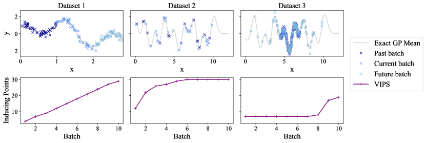
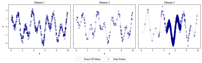
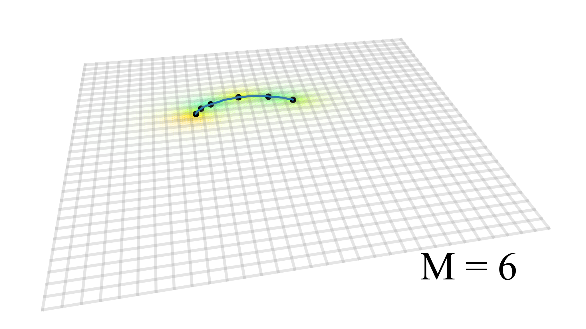
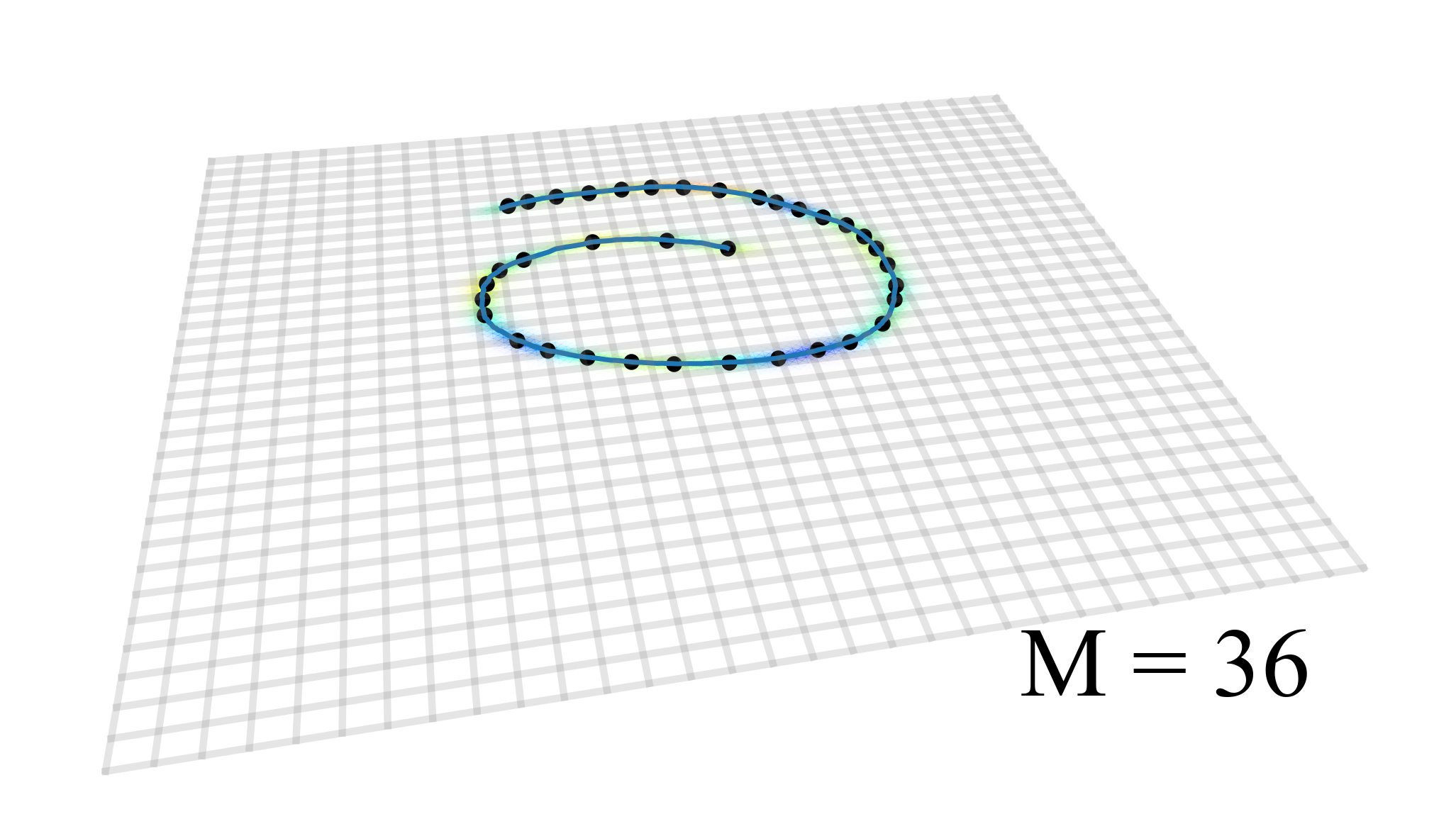
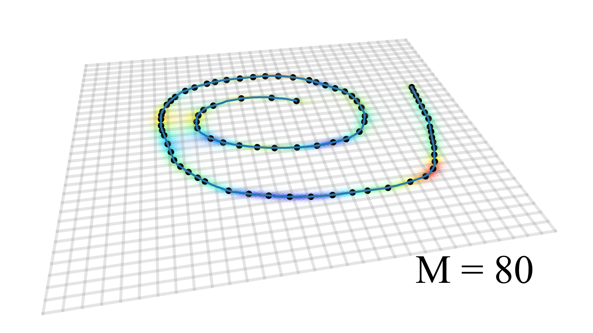
In the experiment, we aim to illustrate the impact of data distribution on the model’s size requirement during continual learning. In Figure 1, we consider three different datasets, each divided into 10 batches, and record the total number of inducing points selected at each batch by our inducing point method, VIPS. In the first scenario, the model encounters a growing input space, leading to a linear increase in the model’s capacity with each batch. In the second, the data distribution remains consistent across batches. After initial learning, the number of inducing points asymptotes to the constant value $M=30$. In the third scenario, the data is concentrated in a part of the input space with occasional outliers in the last batches. Using a large model from the beginning would be a waste of resources. In contrast, our method maintains a low model size for most batches and only increases dynamically when encountering outliers. These scenarios show VIPS’ ability to manage model size across different data distributions during continual learning. See Appendix F.1 for details.

5.2 Speed and accuracy

In continual learning scenarios, manually setting the appropriate number of inducing points beforehand is not possible since this depends on dataset properties and total data points. Fixed-memory approaches can lead to suboptimal performance if the inducing point set is too small, or computational waste if the model is too large. The following two experiments demonstrate these limitations. In contrast, our proposed method VIPS only increases the number of inducing points as needed, highlighting the importance of an adaptive number of inducing points in continual learning.

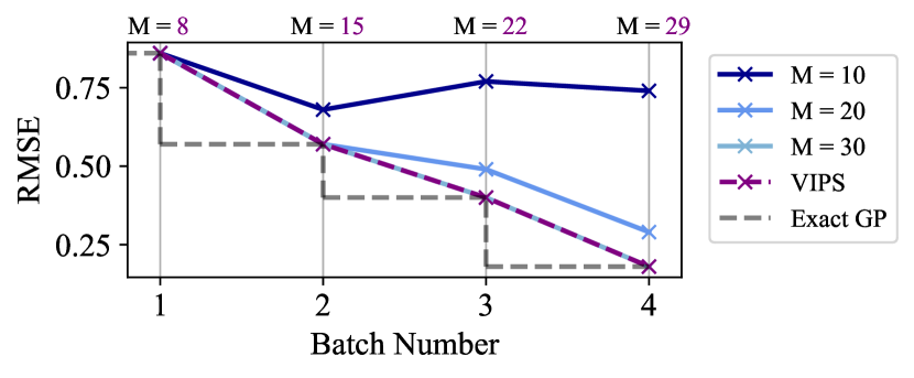
Synthetic data. We compare adaptive and fixed memory methods using a synthetic dataset divided into four equal batches. We evaluate the "greedy variance" location selection method [3] under two scenarios: with a fixed number of inducing points and using our stopping criterion to determine the number of inducing points. We consider three fixed settings ($M=10$, $20$, $30$ total number of inducing points per batch) and record the root mean square error (RMSE) on a test set, using an exact GP model with access to all current training data as a benchmark. Figure 2(a) shows that fixed memory methods with 10 and 20 inducing points become less accurate as more data is observed, while our method VIPS maintains accuracy at each batch. Both the fixed memory method with $M=30$ and VIPS match the performance of an exact GP. This demonstrates the importance of model size in continual learning and the need for adaptive methods to determine the number of inducing points.

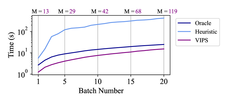
Naval dataset. We compare the time complexity of the location selection method “greedy variance” [3] under three scenarios. In the first scenario, we assume we have access to an oracle to determine the required number of inducing points for near-exact performance, and we set $M=100$ based on the accuracy obtained on a sparse model compared to an exact GP. In the second scenario, we take a heuristic with a large memory ($M=1000$, around 1/10th of the total data points) to ensure sufficient capacity. In the third scenario, we use our method VIPS to determine the number of inducing points. We use the “naval” UCI dataset divided into 20 batches and record the training time per batch. Figure 2(b) shows that both fixed-memory approaches have higher computational time. In contrast, our VIPS method adaptively adjusts $M$ as needed, leading to a reduction in training time.

Overall these simple experiments aim to demonstrate the advantages of adaptive strategies over fixed approaches, achieving high-quality approximation without wasting computational resources.

5.3 UCI datasets

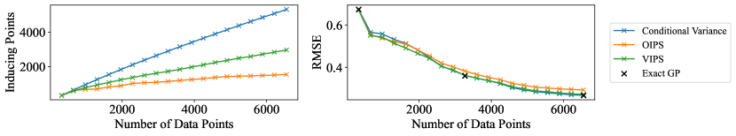
We compare our inducing point selection method, VIPS, to two other adaptive approaches that iteratively choose the number of inducing points with different stopping criteria: Conditional Variance [3] and OIPS [14]. Technical details of these methods are provided in Appendix E.

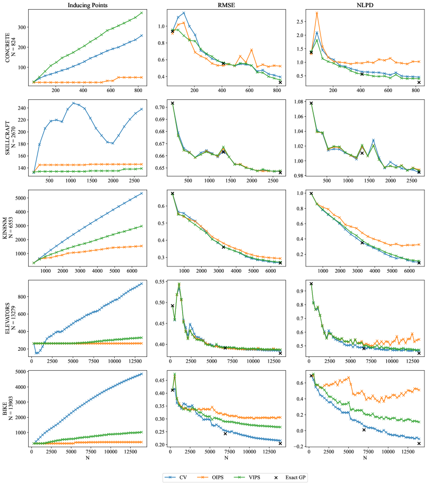
We evaluate five datasets from the UCI repository [8], simulating a streaming scenario by sorting the data based on the first dimension and dividing it into batches. Results are reported over five 80%-training and 20%-testing random splits, including root mean square error (RMSE) and negative log predictive density (NLPD). For Conditional Variance, we set $\eta=0.1$, a threshold that consistently achieves good accuracy across different datasets, and for OIPS, we use default parameters, $\rho=0.8$. For VIPS, we set $\delta=0.05$. Table 1 summarises the last batch results for each dataset in terms of inducing points and RMSE, with an exact GP as a benchmark. Conditional Variance typically selects a higher number of inducing points, while OIPS tends to select the fewest, sometimes compromising accuracy. In contrast, our method achieves a balanced selection of inducing points, maintaining comparable accuracy levels to the other methods, with a single parameter setting performing well across all datasets. Figure 3 exemplifies this, showing how our method maintains accuracy with a prudent selection of inducing points. See Appendix F.3 for the rest of the datasets.

Table 1: UCI datasets: Mean (std) over different training/test splits of the number of inducing points (M) and RMSE for the last batch.
Dataset Exact GP Cond. Variance [3] OIPS [14] VIPS (Ours)
RMSE M RMSE M RMSE M RMSE
Concrete .33(.01) 258(85) .4(.03) 50(19) .52(.02) 371(93) .36(.03)
Skillcraft .65(.03) 238(32) .65(.03) 146(25) .65(.03) 139(2) .65(.03)
Kin8nm .27(.00) 5325(22) .27(.00) 1539(183) .29(.01) 2967(31) .27(.01)
Elevators .38(.00) 949(21) .39(.00) 264(0) .39(.01) 329(2) .39(.00)
Bike .20(.00) 4851(42) .22(.00) 366(44) .31(.01) 1021(14) .27(.00)
Refer to caption
Figure 3: Plot of the selected number of inducing points and RMSE versus the number of data points observed for different inducing point selection methods using the UCI dataset “kin8nm”. The exact GP which has access to all observations is added as a benchmark for first, middle and last batch.

5.4 Magnetic Anomalies

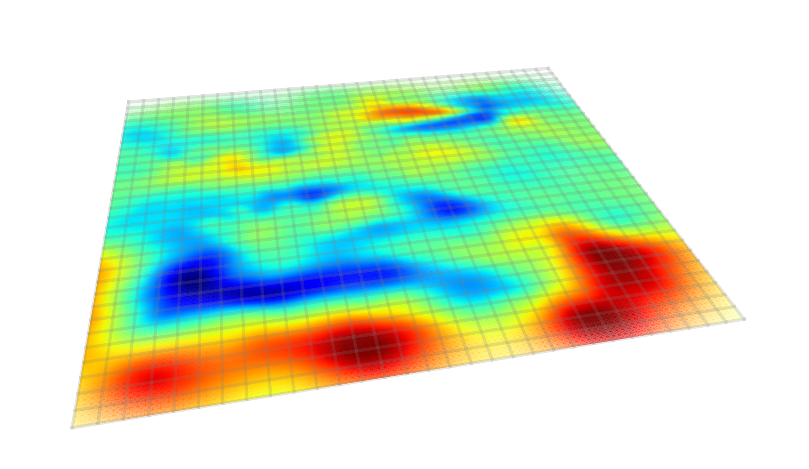
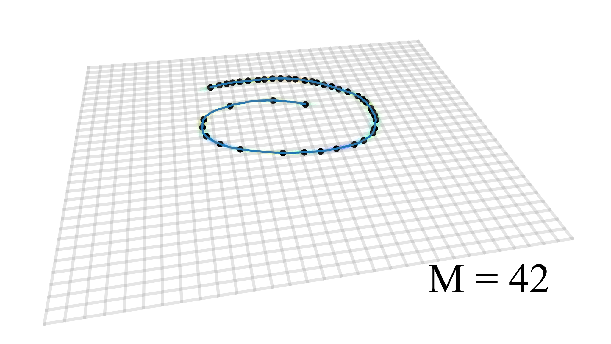
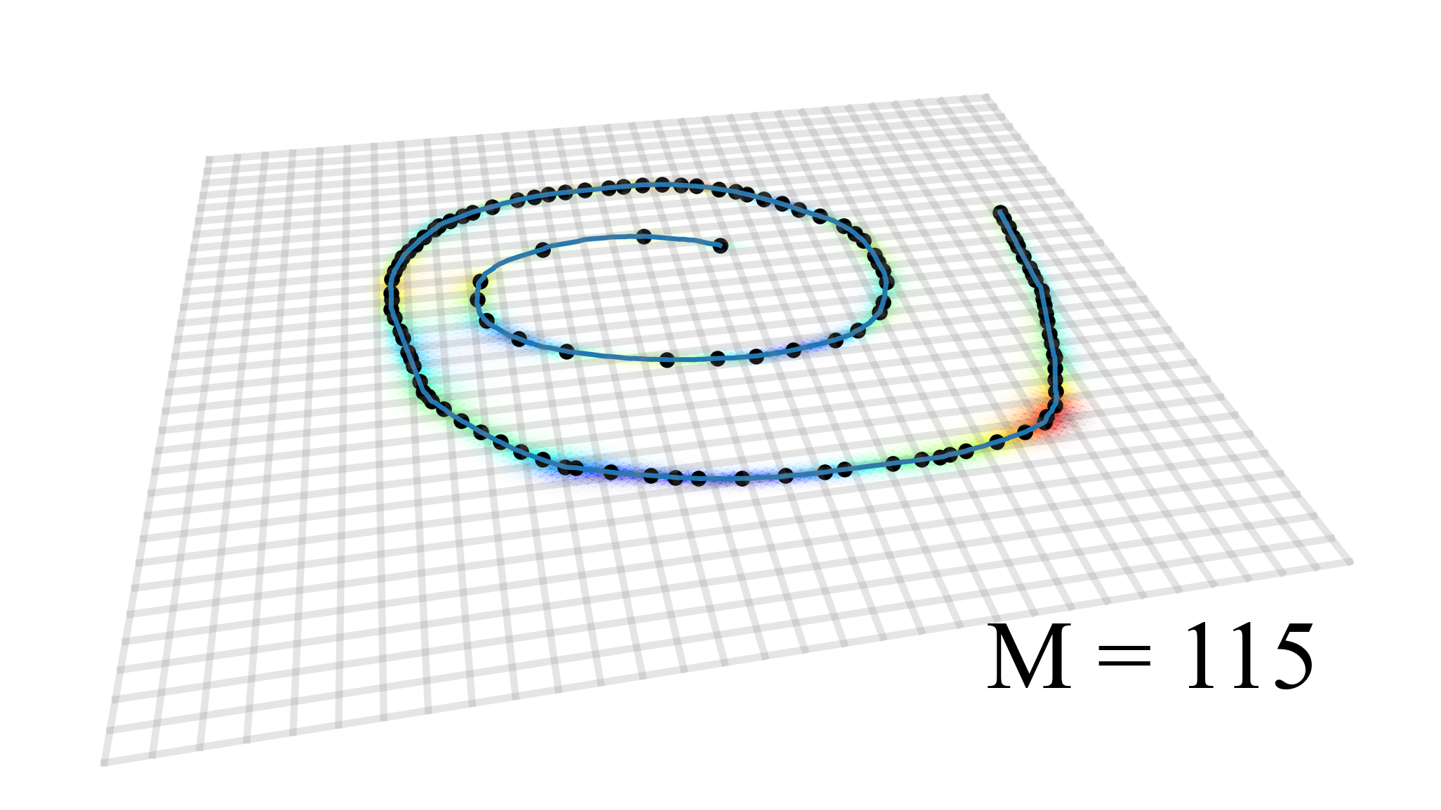
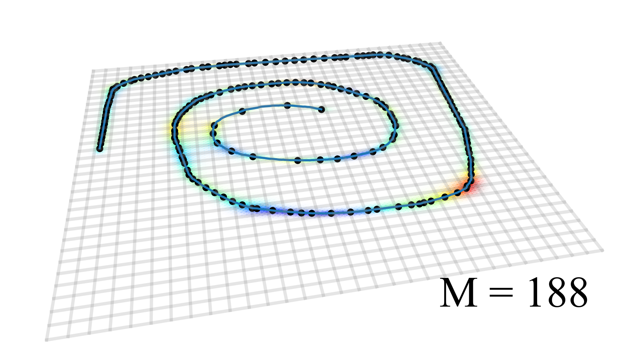
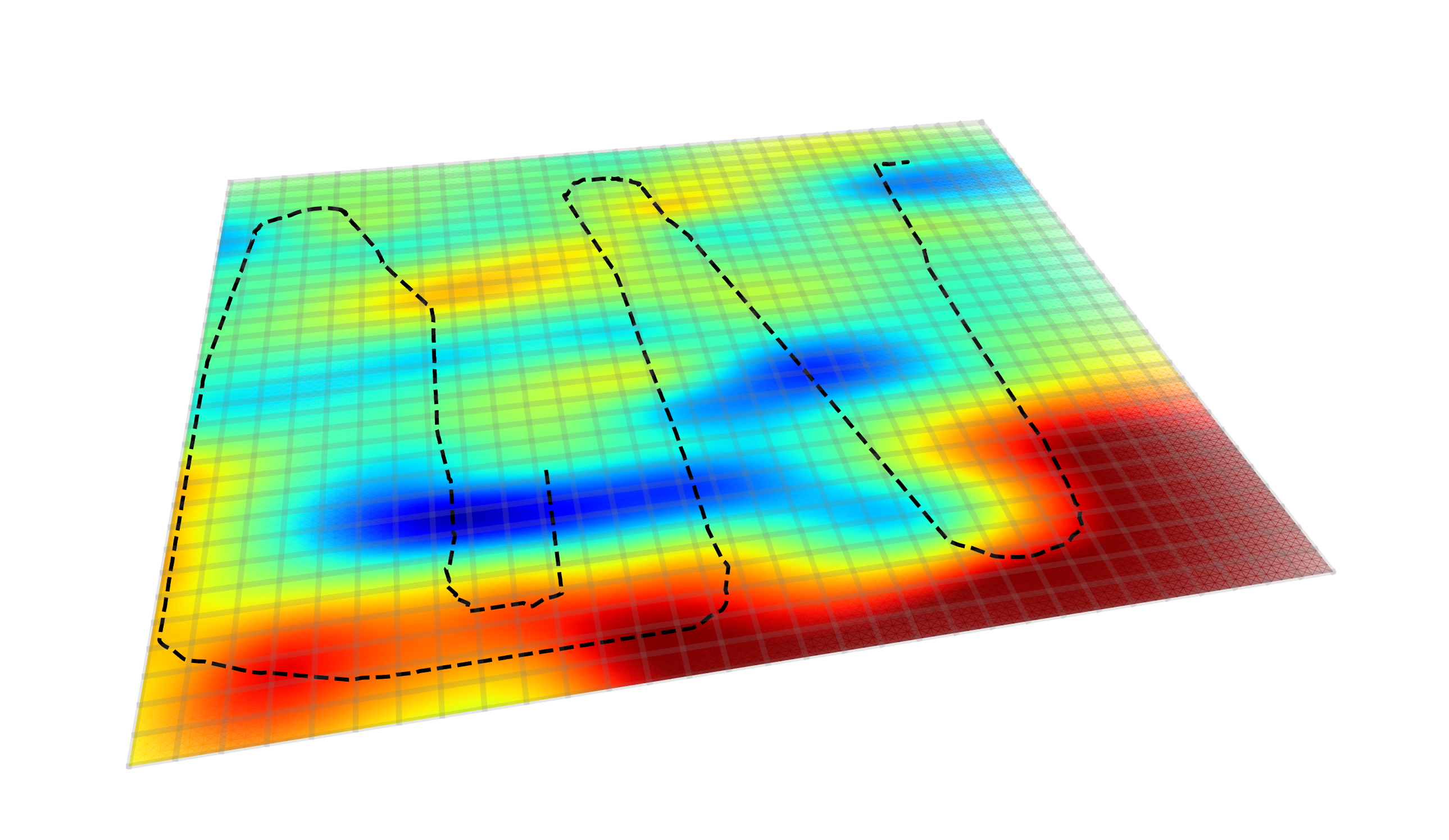
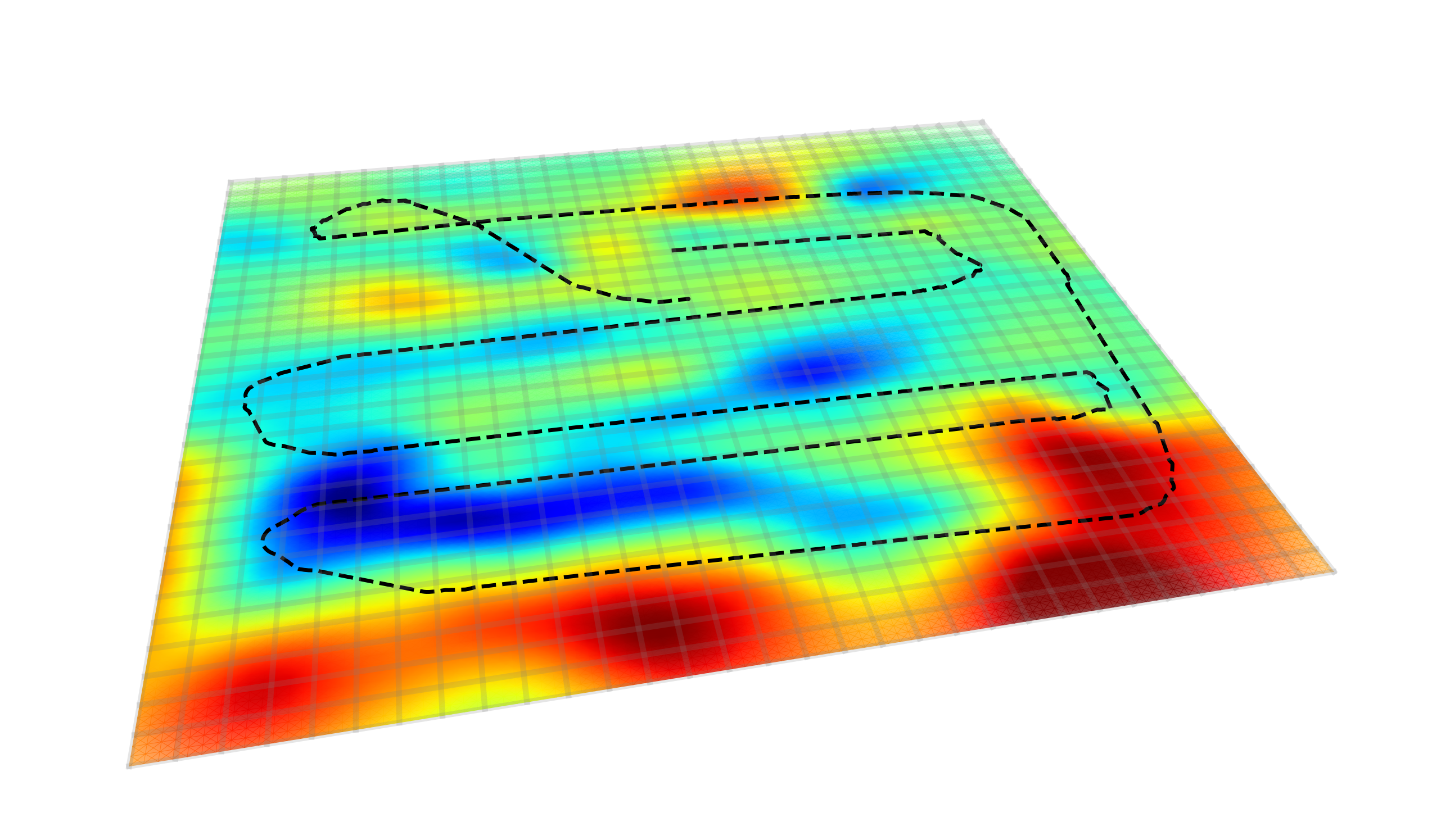
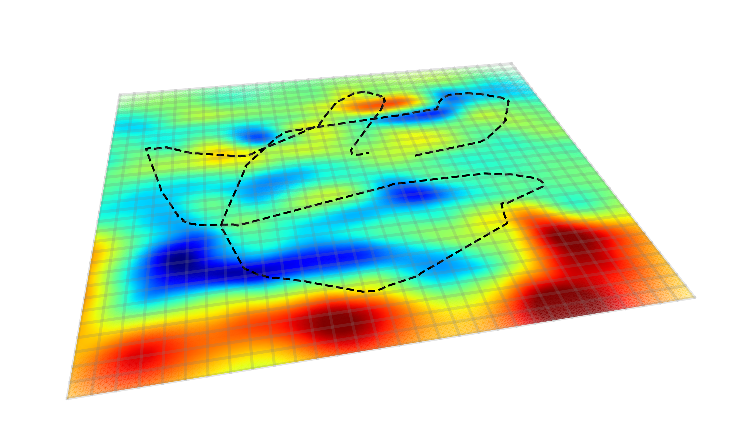
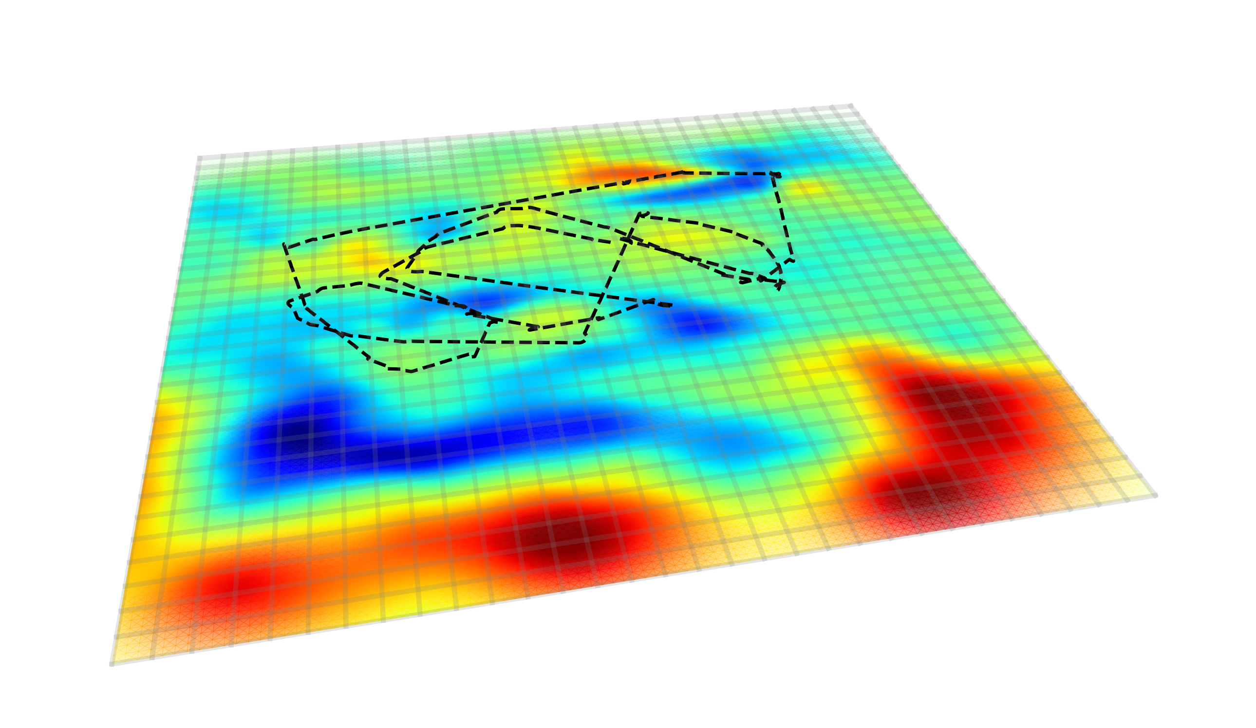
Finally, we consider the experimental setup described by Chang et al. [4] and the real-world data from Solin et al. [39], where a small wheeled robot with a 3-axis magnetometer navigates a 6m x 6m indoor space to map magnetic field anomalies online. This experiment mimics a real-world setting with an ever-expanding domain, where the robot is not confined to a predefined area. In this context, restricting the model’s capacity is impractical since we need to learn new parts of the space continuously. This requires a method that can accommodate new data without uncontrollably increasing the model’s capacity.

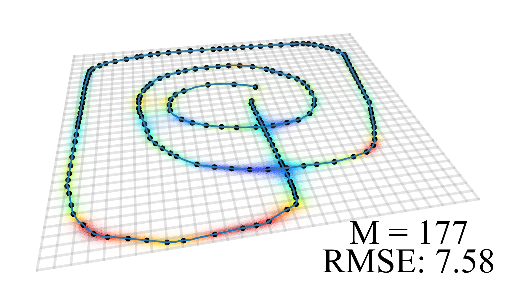
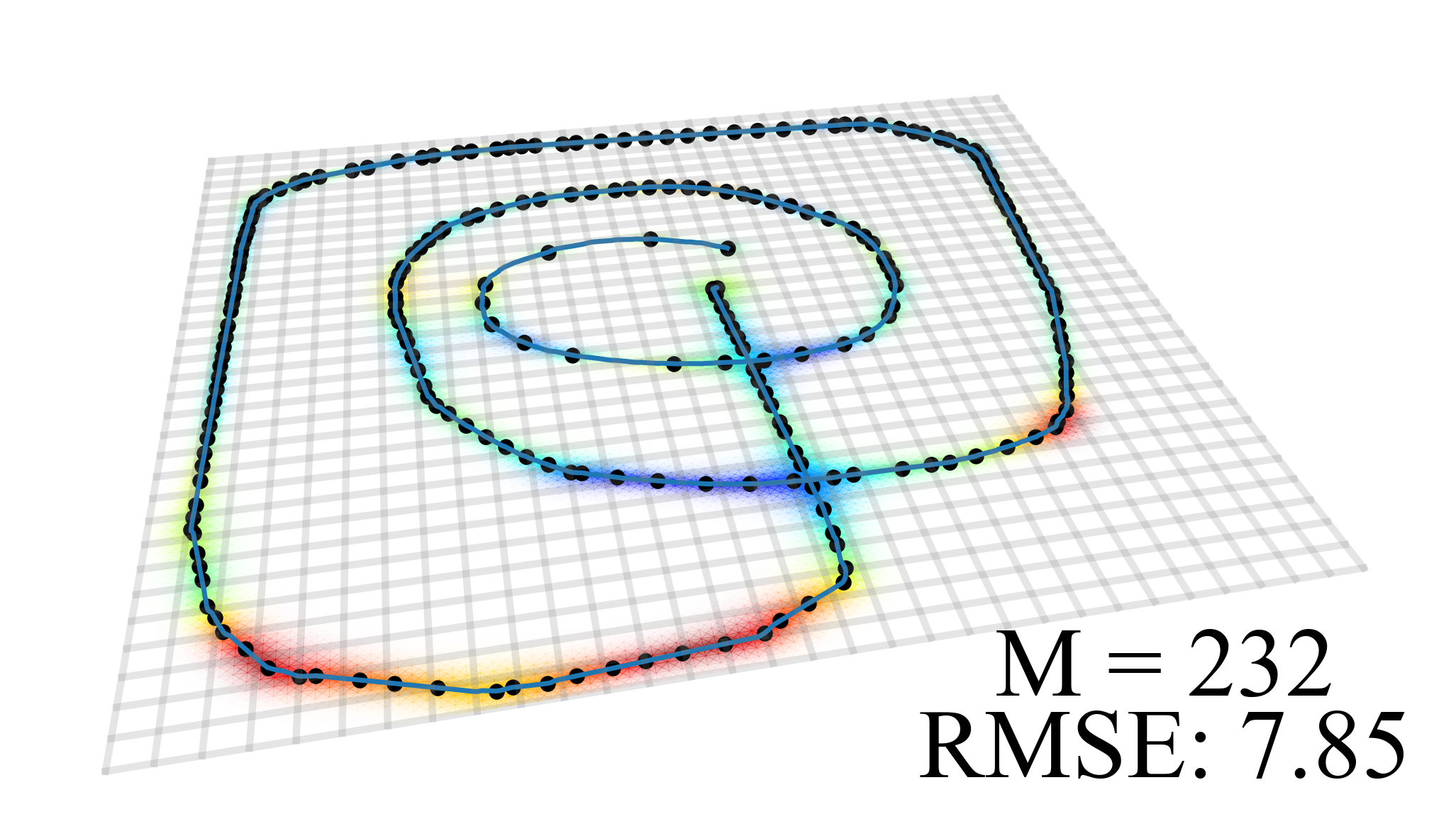
We explore two approaches for learning the robot’s path. In the first approach, each batch represents a complete path taken by the robot. Figure 4(a) shows the final magnetic field estimate after learning from all paths with the marginal variance controlling the opacity. Our method achieves an accurate representation by dynamically adjusting the inducing points. In the second approach, the robot’s path is processed in continuous batches as it moves forward. Figures 4(c) and 4(b) display the mean estimates for the final batch using our method VIPS and Conditional Variance. Our method produces a similar local estimate to Figure 4(a), uses fewer inducing points than Conditional Variance to achieve similar accuracy and does not require hyperparameter tuning. See Appendix F.4 for more details and results.

Refer to caption
(a) Learning paths sequentially.
Refer to caption
(b) VIPS (Ours).
Refer to caption
(c) Conditional Variance
Figure 4: A small robot is used to perform sequential estimation of magnetic field anomalies. The strength of the magnetic field is given by 10 $\mu\mathrm{T}$ to 90 $\mu\mathrm{T}$. (a)-(b) show the outcome of learning when data for a single path is received continuously. (c) shows the final estimate of the magnitude field learned sequentially through different paths.

6 Discussion

In this work, we introduce a principled approach for determining the number of inducing points required in streaming sparse GP regression. Unlike conventional methods that rely on a fixed number of inducing points, our approach automatically adjusts the number of inducing points and offers an accuracy guarantee through user-controlled parameters. Our approach effectively eliminates the need to specify a “size” hyperparameter upfront, thereby addressing a significant bottleneck in traditional methods. This allows a GP to be trained without compromising performance due to insufficient memory or wasting computational resources with an unnecessarily large memory allocation. While our current application focuses on GPs we hope this is extendable for the development of adaptive Neural Networks.

References

  • Bauer et al. [2016] M. Bauer, M. van der Wilk, and C. E. Rasmussen. Understanding probabilistic sparse Gaussian process approximations. Advances in neural information processing systems, 29, 2016.
  • Bui et al. [2017] T. D. Bui, C. Nguyen, and R. E. Turner. Streaming sparse gaussian process approximations. Advances in Neural Information Processing Systems, 30:3299–3307, 2017. ISSN 1049-5258.
  • Burt et al. [2020] D. R. Burt, C. E. Rasmussen, and M. van der Wilk. Convergence of sparse variational inference in Gaussian processes regression. The Journal of Machine Learning Research, 21(1):5120–5182, 2020.
  • Chang et al. [2023a] P. E. Chang, P. Verma, S. John, A. Solin, and M. E. Khan. Memory-Based dual gaussian processes for sequential learning. In International Conference on Machine Learning, pages 4035–4054. PMLR, June 2023a.
  • Chang et al. [2023b] P. G. Chang, G. Durán-Martín, A. Shestopaloff, M. Jones, and K. P. Murphy. Low-rank extended kalman filtering for online learning of neural networks from streaming data. pages 1025–1071, 2023b.
  • Cho and Saul [2009] Y. Cho and L. Saul. Kernel methods for deep learning. Advances in neural information processing systems, 22, 2009.
  • Cover [1999] T. M. Cover. Elements of information theory, page 14. John Wiley & Sons, 1999.
  • Dua and Graff [2017] D. Dua and C. Graff. UCI machine learning repository, 2017. URL http://archive.ics.uci.edu/ml.
  • Dutordoir et al. [2020] V. Dutordoir, N. Durrande, and J. Hensman. Sparse gaussian processes with spherical harmonic features. In International Conference on Machine Learning, pages 2793–2802. PMLR, 2020.
  • Dutordoir et al. [2021] V. Dutordoir, J. Hensman, M. van der Wilk, C. H. Ek, Z. Ghahramani, and N. Durrande. Deep neural networks as point estimates for deep gaussian processes. Advances in Neural Information Processing Systems, 34:9443–9455, 2021.
  • Farquhar and Gal [2018] S. Farquhar and Y. Gal. Towards robust evaluations of continual learning. arXiv preprint arXiv:1805.09733, 2018.
  • Fine and Scheinberg [2001] S. Fine and K. Scheinberg. Efficient svm training using low-rank kernel representations. Journal of Machine Learning Research, 2(Dec):243–264, 2001.
  • Foster et al. [2009] L. Foster, A. Waagen, N. Aijaz, M. Hurley, A. Luis, J. Rinsky, C. Satyavolu, M. J. Way, P. Gazis, and A. Srivastava. Stable and efficient gaussian process calculations. Journal of Machine Learning Research, 10(4), 2009.
  • Galy-Fajou and Opper [2021] T. Galy-Fajou and M. Opper. Adaptive inducing points selection for Gaussian Processes. In Continual Learning Workshop, July 2021.
  • Ghahramani [2013] Z. Ghahramani. Bayesian non-parametrics and the probabilistic approach to modelling. Philosophical Transactions of the Royal Society A: Mathematical, Physical and Engineering Sciences, 371(1984):20110553, 2013.
  • Ghahramani [2015] Z. Ghahramani. Probabilistic machine learning and artificial intelligence. Nature, 521(7553):452–459, 2015.
  • Goodfellow et al. [2013] I. J. Goodfellow, M. Mirza, D. Xiao, A. Courville, and Y. Bengio. An empirical investigation of catastrophic forgetting in gradient-based neural networks. arXiv preprint arXiv:1312.6211, 2013.
  • Grünwald and Roos [2019] P. Grünwald and T. Roos. Minimum description length revisited. International journal of mathematics for industry, 11(01):1930001, 2019.
  • Kapoor et al. [2021] S. Kapoor, T. Karaletsos, and T. D. Bui. Variational auto-regressive gaussian processes for continual learning. In International Conference on Machine Learning, pages 5290–5300. PMLR, 2021.
  • Kessler et al. [2021] S. Kessler, V. Nguyen, S. Zohren, and S. J. Roberts. Hierarchical indian buffet neural networks for bayesian continual learning. In Uncertainty in artificial intelligence, pages 749–759. PMLR, 2021.
  • Kirkpatrick et al. [2017] J. Kirkpatrick, R. Pascanu, N. Rabinowitz, J. Veness, G. Desjardins, A. A. Rusu, K. Milan, J. Quan, T. Ramalho, A. Grabska-Barwinska, et al. Overcoming catastrophic forgetting in neural networks. Proceedings of the national academy of sciences, 114(13):3521–3526, 2017.
  • Li and Hoiem [2017] Z. Li and D. Hoiem. Learning without forgetting. IEEE transactions on pattern analysis and machine intelligence, 40(12):2935–2947, 2017.
  • Lopez-Paz and Ranzato [2017] D. Lopez-Paz and M. Ranzato. Gradient episodic memory for continual learning. Advances in neural information processing systems, 30, 2017.
  • Maddox et al. [2021] W. J. Maddox, S. Stanton, and A. G. Wilson. Conditioning sparse variational gaussian processes for online decision-making. Advances in Neural Information Processing Systems, 34:6365–6379, 2021.
  • Matthews [2017] A. G. d. G. Matthews. Scalable Gaussian process inference using variational methods. PhD thesis, 2017.
  • Matthews et al. [2016] A. G. d. G. Matthews, J. Hensman, R. Turner, and Z. Ghahramani. On sparse variational methods and the Kullback-Leibler divergence between stochastic processes. In A. Gretton and C. C. Robert, editors, Proceedings of the 19th International Conference on Artificial Intelligence and Statistics, volume 51 of Proceedings of Machine Learning Research, pages 231–239, Cadiz, Spain, 2016. PMLR.
  • Matthews et al. [2018] A. G. d. G. Matthews, J. Hron, M. Rowland, R. E. Turner, and Z. Ghahramani. Gaussian process behaviour in wide deep neural networks. In International Conference on Learning Representations, 2018.
  • McCloskey and Cohen [1989] M. McCloskey and N. J. Cohen. Catastrophic interference in connectionist networks: The sequential learning problem. In Psychology of learning and motivation, volume 24, pages 109–165. Elsevier, 1989.
  • Motwani and Raghavan [1995] R. Motwani and P. Raghavan. Randomized Algorithms. Cambridge University Press, 1995.
  • Murphy [2023] K. P. Murphy. Probabilistic Machine Learning: Advanced Topics, chapter 29.7.2. MIT Press, 2023.
  • Neal [1996] R. M. Neal. Bayesian learning for neural networks, volume 118. Springer Science & Business Media, 1996.
  • Nguyen et al. [2018] C. V. Nguyen, Y. Li, T. D. Bui, and R. E. Turner. Variational continual learning. In International Conference on Learning Representations, Oct. 2018.
  • Panos et al. [2018] A. Panos, P. Dellaportas, and M. K. Titsias. Fully scalable gaussian processes using subspace inducing inputs. arXiv preprint arXiv:1807.02537, 2018.
  • Rasmussen and Williams [2005] C. E. Rasmussen and C. K. I. Williams. Gaussian Processes for Machine Learning. MIT Press, Nov. 2005. ISBN 9780262182539.
  • Ring [1997] M. B. Ring. Child: A first step towards continual learning. Machine Learning, 28(1):77–104, 1997.
  • Rudner et al. [2022] T. G. Rudner, F. B. Smith, Q. Feng, Y. W. Teh, and Y. Gal. Continual learning via sequential function-space variational inference. In International Conference on Machine Learning, pages 18871–18887. PMLR, 2022.
  • Rusu et al. [2016] A. A. Rusu, N. C. Rabinowitz, G. Desjardins, H. Soyer, J. Kirkpatrick, K. Kavukcuoglu, R. Pascanu, and R. Hadsell. Progressive neural networks. arXiv preprint arXiv:1606.04671, 2016.
  • Schwarz et al. [2018] J. Schwarz, W. Czarnecki, J. Luketina, A. Grabska-Barwinska, Y. W. Teh, R. Pascanu, and R. Hadsell. Progress & compress: A scalable framework for continual learning. In International conference on machine learning, pages 4528–4537. PMLR, 2018.
  • Solin et al. [2018] A. Solin, M. Kok, N. Wahlstrom, T. Schon, and S. Sarkka. Modeling and interpolation of the ambient magnetic field by gaussian processes. IEEE Transactions on Robotics, 34(4):1112–1127, 2018. ISSN 1552-3098. doi: 10.1109/TRO.2018.2830326.
  • Sun et al. [2020] S. Sun, J. Shi, and R. B. Grosse. Neural networks as inter-domain inducing points. In Third Symposium on Advances in Approximate Bayesian Inference, 2020.
  • Titsias [2009] M. K. Titsias. Variational learning of inducing variables in sparse gaussian processes. In Proceedings of the Twelfth International Conference on Artificial Intelligence and Statistics (AISTATS), volume 5 of Proceedings of Machine Learning Research, pages 567–574. PMLR, 2009.
  • Titsias [2014] M. K. Titsias. Variational inference for Gaussian and determinantal point processes. In Workshop on Advances in Variational Inference (NIPS), 2014.
  • van der Vaart and van Zanten [2008] A. van der Vaart and J. van Zanten. Rates of contraction of posterior distributions based on gaussian process priors. The Annals of Statistics, 36(3):1435–1463, 2008.
  • van der Wilk [2019] M. van der Wilk. Sparse Gaussian process approximations and applications. PhD thesis, 2019.
  • Yoon et al. [2018] J. Yoon, E. Yang, J. Lee, and S. J. Hwang. Lifelong learning with dynamically expandable networks. In 6th International Conference on Learning Representations, ICLR 2018. International Conference on Learning Representations, ICLR, 2018.

Appendix A Societal Impact

This paper presents work whose goal is to advance the field of Machine Learning. There are many potential societal consequences of our work, none of which we feel must be specifically highlighted here.

Appendix B Code

The methods discussed in this work, along with the code to reproduce our results, are available online at https://github.com/guiomarpescador/vips.

Appendix C Vegas Inducing Point Selection (VIPS) Algorithm

Algorithm 1 Vegas Inducing Point Selection (VIPS)
  Input: $\mathbf{X}_{n}=\{\mathbf{x}_{i}\}_{i=1}^{N_{n}}$, $\mathbf{Z}_{o}=\{\mathbf{z}_{m}\}_{m=1}^{M_{\mathbf{a}}}$, $\hat{\mu}$, $\hat{\sigma}$, $\theta_{n}$, kernel $k(\cdot,\cdot|\theta_{n})$, threshold parameter $\delta$.
  Output: Updated set $\mathbf{Z}_{n}=\mathbf{Z}_{o}\cup\{\mathbf{x}_{m^{\prime}}\}_{m^{\prime}=1}^{M_{\mathbf{b}}}$.
  Initialise $\mathbf{Z}_{n}=\mathbf{Z}_{o}$.
  while $\widehat{\mathcal{U}}(M)-\widehat{\mathcal{L}}(M_{\mathbf{b}})\geq\delta|\widehat{\mathcal{U}}(M)-\mathcal{L}_{noise}(\hat{\mu},\hat{\sigma})|$ do
    Select $\mathbf{x}={\operatorname{argmax}}_{\mathbf{x}\in\mathbf{X}_{n}}\,k(\mathbf{x},\mathbf{x})-\mathbf{k}_{\mathbf{b}}(\mathbf{x})^{\top}\mathbf{K}_{\mathbf{bb}}^{-1}\mathbf{k}_{\mathbf{b}}(\mathbf{x})$.
    Add $\mathbf{x}$ to the set of inducing points: $\mathbf{Z}_{n}=\mathbf{Z}_{n}\cup\{\mathbf{x}\}$.
  end while

Algorithm 1 presents an inducing point selection method using our stopping criterion combined with the location selection strategy “greedy variance” [3, 12, 13]. At each batch, we keep the old inducing point locations fixed and choose the new set of inducing points from among the locations in $\mathbf{X}_{n}$. The method takes as input a value for the hyperparameter $\theta_{n}$. In practice, we will set $\theta_{n}=\theta_{o}$ to select the number of inducing points; the hyperparameter $\theta_{n}$ is inferred by optimising $\widehat{\mathcal{L}}(M_{\mathbf{b}})$ once the inducing point locations $\mathbf{Z}_{n}$ has been chosen.

Appendix D Proof of Guarantee

Guarantee.

Let $M$ be a fixed integer and $M_{\mathbf{b}}$ be the number of selected inducing points such that $\widehat{\mathcal{U}}(M)-\widehat{\mathcal{L}}(M_{\mathbf{b}})\leq\alpha$. Assuming that $\theta_{n}=\theta_{o}$, we have two equivalent bounds:

$\displaystyle\operatorname{KL}[q_{n}(f)\mid\mid p(f|\mathbf{y}_{o},\mathbf{y}_{n},\theta_{o})]$ $\displaystyle\leq\alpha+\Psi$ (22)
$\displaystyle\mathrm{KL}[q_{n}(f)\mid\mid q_{n}^{*}(f)]$ $\displaystyle\leq\alpha$ (23)

where $\Psi=\int q_{n}(f)\log\frac{q_{n}^{*}(f)}{p(f|\mathbf{y}_{n},\mathbf{y}_{o})}\mathrm{d}f$ and $q_{n}^{*}(f)=\mathcal{Z}^{-1}q_{o}(f)p(\mathbf{y}_{n}|f)$ represents the variational distribution associated with the optimal lower bound $\mathcal{L}^{*}=\widehat{\mathcal{L}}(N_{n}+M_{\mathbf{a}})$, with $\mathcal{Z}$ denoting the marginal likelihood that normalises $q_{n}^{*}(f)$.

Proof.

We cease the addition of points when $\widehat{\mathcal{U}}(M)-\widehat{\mathcal{L}}(M_{\mathbf{b}})<\alpha$. Since $\widehat{\mathcal{U}}(M)\geq\mathcal{L}^{*}$, then $-\widehat{\mathcal{L}}(M_{\mathbf{b}})<\alpha-\widehat{\mathcal{U}}(M)<\alpha-\mathcal{L}^{*}$. Assuming $\theta_{n}=\theta_{o}$, eq. (4) can be bounded as:

$\displaystyle\operatorname{KL}[q_{n}(f)\mid\mid p(f|\mathbf{y}_{o},\mathbf{y}_{n},\theta_{n})]$ $\displaystyle=\log p(\mathbf{y}_{n}|\mathbf{y}_{o})-\widehat{\mathcal{L}}+\Phi$ (24)
$\displaystyle\leq\log p(\mathbf{y}_{n}|\mathbf{y}_{o})+\alpha-\mathcal{L}^{*}+\Phi$

where $\Phi=-\int q_{n}(f)\log\frac{p(f|\mathbf{y}_{o},\theta_{o})}{q_{o}(f)}\text{d}f$. Let $q_{n}^{*}(f)=\mathcal{Z}^{-1}q_{o}(f)p(\mathbf{y}_{n}|f)$ be the variational distribution associated with $\mathcal{L}^{*}=\widehat{\mathcal{L}}(N_{n}+M_{\bf a})$, then by multiplying this value in both sides of the fraction inside the log, we obtain:

$\displaystyle\Phi$ $\displaystyle=\int q_{n}(f)\log\frac{q_{o}(f)}{p(f|\mathbf{y}_{o})}\text{d}f$ (25)
$\displaystyle=\int q_{n}(f)\log\frac{q_{o}(f)}{p(f|\mathbf{y}_{o})}\frac{q_{n}^{*}(f)}{q_{n}^{*}(f)}\text{d}f$
$\displaystyle=\int q_{n}(f)\log\frac{q_{o}(f)}{p(f|\mathbf{y}_{o})}\frac{q_{n}^{*}(f)}{\mathcal{Z}^{-1}q_{o}(f)p(\mathbf{y}_{n}|f)}\text{d}f$
$\displaystyle=\int q_{n}(f)\log\frac{q_{n}^{*}(f)}{p(f|\mathbf{y}_{n},\mathbf{y}_{o})p(\mathbf{y}_{n}|\mathbf{y}_{o})}\text{d}f+\log\mathcal{Z}$
$\displaystyle=\int q_{n}(f)\log\frac{q_{n}^{*}(f)}{p(f|\mathbf{y}_{n},\mathbf{y}_{o})}\text{d}f+\log\mathcal{Z}-\log p(\mathbf{y}_{n}\mid\mathbf{y}_{o})$

Then we can rewrite,

$\displaystyle\operatorname{KL}[q_{n}(f)\mid\mid p(f|\mathbf{y}_{o},\mathbf{y}_{n},\theta_{o})]$ (26)
$\displaystyle\quad\leq\log p(\mathbf{y}_{n}|\mathbf{y}_{o},\theta_{n})+\alpha-\mathcal{L}^{*}+\Phi$
$\displaystyle\quad\leq\log p(\mathbf{y}_{n}|\mathbf{y}_{o})+\alpha-\mathcal{L}^{*}+\int q_{n}(f)\log\frac{q_{n}^{*}(f)}{p(f|\mathbf{y}_{n},\mathbf{y}_{o},\theta_{n})}\text{d}f+\log\mathcal{Z}-\log p(\mathbf{y}_{n}\mid\mathbf{y}_{o})$
$\displaystyle\quad\leq\alpha+\int q_{n}(f)\log\frac{q_{n}^{*}(f)}{p(f|\mathbf{y}_{n},\mathbf{y}_{o},\theta_{n})}\text{d}f$

Again by multiplying by $q_{n}(f)$ both sides of the fraction inside the log, we obtain:

$\displaystyle\operatorname{KL}[q_{n}(f)\mid\mid p(f|\mathbf{y}_{o},\mathbf{y}_{n},\theta_{o})]$ $\displaystyle\leq\int q_{n}(f)\log\frac{q_{n}^{*}(f)}{p(f|\mathbf{y}_{n},\mathbf{y}_{o},\theta_{n})}\frac{q_{n}(f)}{q_{n}(f)}\text{d}f+\alpha$ (27)
$\displaystyle\operatorname{KL}[q_{n}(f)\mid\mid p(f|\mathbf{y}_{o},\mathbf{y}_{n},\theta_{n})]$ $\displaystyle\leq\operatorname{KL}[q_{n}(f)\mid\mid p(f|\mathbf{y}_{o},\mathbf{y}_{n},\theta_{n})]-\operatorname{KL}[q_{n}(f)\mid\mid q_{n}^{*}(f)]+\alpha$
$\displaystyle\operatorname{KL}[q_{n}(f)\mid\mid q_{n}^{*}(f)]$ $\displaystyle\leq\alpha$

Appendix E Inducing Points Selection Methods

The effectiveness of sparse approximations is determined by two key factors: the number of inducing points ($M$) and their locations. These parameters are responsible for a trade-off between the scalability and accuracy of the model, thus representing the captured information about the function $f$ [3, 24]. There exist multiple approaches to inducing point selection (see Burt et al. [3] for a review), broadly falling into two categories.

The first category includes choosing a subset of the input data through sampling or clustering and refining their location during gradient optimisation of the ELBO. For instance, Bui et al. [2] decided to sample a fixed number of inducing points from the set $\{Z_{o},X_{n}\}$ and optimise their locations. However, this approach uses a fixed memory, which requires a manual setting of the number of inducing points. Determining the memory size is inherently challenging as it will depend on the dataset’s properties and the estimated number of data points, not possible to know in advance.

In the second approach, points are iteratively selected from a set based on a specific criterion. Burt et al. [3] introduced an iterative "greedy variance" strategy that greedily chooses the location of the next inducing point to maximize the marginal variance in the conditional prior $p(f_{\neq\mathbf{u}}|\mathbf{u})$. This is equivalent to maximising $\operatorname{diag}[\mathbf{K_{ff}}-\mathbf{Q_{ff}}]$. The quantity $\operatorname{tr}\left(\mathbf{K_{ff}}-\mathbf{Q_{ff}}\right)$ is a bound for the norm of $\mathbf{K_{ff}}-\mathbf{Q_{ff}}$, and can therefore be used as a stopping criterion to determine the number of inducing points. We refer to the method that uses "greedy variance" with this stopping criterion as Conditional Variance. In this algorithm, new inducing points are no longer added once $\operatorname{tr}\left(\mathbf{K_{ff}}-\mathbf{Q_{ff}}\right)$ falls below a chosen tolerance value $\eta$. Although, an equivalent approach was studied in Fine and Scheinberg [12] and Foster et al. [13], this stopping criterion has not yet been tested in the literature. In the online setting, Chang et al. [4] use the “greedy variance” criterion by simply defining $\{\mathbf{Z}_{o},\mathbf{X}_{n}\}$ as the selection pool from which inducing point locations are selected, however, they maintain a fixed number of inducing points. Similarly, Maddox et al. [24] extends the “greedy variance” criterion to heteroskedastic Gaussian likelihoods and also uses a fixed memory approach. Galy-Fajou and Opper [14] introduced the Online Inducing Points Selection (OIPS) algorithm, a method that iteratively adds points from $\mathbf{X}_{n}$ to the existing set of inducing points: a point $\mathbf{x}\in\mathbf{X}_{n}$ is added to the set of inducing points if the maximum value of the covariance vector $\mathbf{k}_{\mathbf{u}}(\mathbf{x})$ is below a set threshold $\rho$. This method measures the potential potential impact of each new point with the existing inducing points set given the covariance threshold, this allows for an automatic selection of the number of inducing points unless a maximum is specified.

In our work, we are not interested in constraining the capacity of the model. Therefore, we will compare our method VIPS, to Conditional Variance with the selection pool ($\{\mathbf{Z}_{o},\mathbf{X}_{n}\}$) and OIPS without specifying a maximum number of inducing points. Table 2 shows a summary of the properties of these methods as well as the fixed memory approach used in Bui et al. [2].

Table 2: Properties of inducing points selection method for updating an online GP regression model.
Method Type Selection Pool Selection Criteria Stopping Criterion
Bui et al. [2] Fixed Random sample Gradient optimisation M constant
Cond. Variance (CV) Adaptive $\{X_{new},Z_{old}\}$ Greedy variance $\operatorname{tr}\left(\mathbf{K_{ff}}-\mathbf{Q_{ff}}\right)\leq\eta$.
OIPS [14] Adaptive $\{X_{new}\}$ $\max\mathbf{k}_{\mathbf{u}}(\mathbf{x})\leq\rho$ All points satisfying selection criteria.
VIPS Adaptive $\{X_{new}\}$ Greedy variance $\widehat{\mathcal{L}}\geq\widehat{\mathcal{U}}-\alpha$

Appendix F Further Experimental Details and Results

For all experiments and methods, we use the L-BFGS optimiser.

F.1 Data types

For the synthetic dataset, we generate random noisy observations from the test function $f(x)=\sin(2x)+\cos(5x)$. We used a Squared Exponential kernel initialised with lengthscale $0.5$ and variance $1$. The noise variance was initialised to $0.5$. For VIPS, we use $\delta=0.05$.

Dataset 1:

We use $N=500$ observations uniformly distributed from 00 to $10$. The data is ordered and divided into ten random batches.

Dataset 2:

We simulate a scenario where small batches of data are received but the data is distributed across the input space. We use $N=150$ observations uniformly distributed from 00 to $10$. The data is shuffled and divided into ten random batches.

Dataset 3:

We simulate a scenario where only outliers are encountered from time to time and the rest of the data is concentrated around a small part of the input space. We use two sets of data: the first set is sampled from a uniform distribution from $4$ to $6$, with $N=1000$ and the second set is sampled from a Cauchy distribution with a mean of $\mu=5$, with $N=300$. The data is divided into ten random batches, where the Cauchy observations are placed in the latter batches.

Refer to caption
Figure 5: Plot of the three datasets considered in Section F.1.

F.2 Speed and Accuracy

F.2.1 Synthetic data

For the synthetic dataset, we generate 1000 random noisy observations from the test function $f(x)=\sin(2x)+\cos(5x)$. We used a Squared Exponential kernel initialised with lengthscale $0.5$ and variance $1.5$. The noise variance was initialised to 0.5. The performance was measured on a test grid of $500$ points. For VIPS, $\delta=0.05$.

F.2.2 Timing

This experiment was performed on an Nvidia RTX 6000’s GPU on a high-performance computing cluster. We used a Squared Exponential kernel with hyperparameters initialised to 1. The noise variance was initialised to 0.1. The dataset was divided into 20 batches, and we recorded the time in training per batch.

F.3 UCI datasets

Table 3: UCI datasets: methods parameters used for each dataset.

Dataset Dimension (N, D) Conditional Variance [3] OIPS [14] VIPS
$\eta$ $\rho$ $\delta$
Concrete 1030, 8 0.1 0.80 0.05
Skillcraft 3338, 19 0.1 0.80 0.05
Kin8nm 8192, 8 0.1 0.80 0.05
Elevators 16599, 18 0.1 0.80 0.05
Bike 17379, 17 0.1 0.80 0.05

These experiments were performed on an Nvidia RTX 6000’s GPU on a high-performance computing cluster. We used a Squared Exponential kernel with hyperparameters initialised to 1 for all datasets. The noise variance was initialised to 0.1. Table 3 shows the parameters used for each dataset and method. The smaller datasets $(<12000)$ were divided into 20 batches, and the larger $(>12000)$ into 50 batches. Figure 6 shows the results for all considered datasets. As mentioned in the main text, the method Conditional Variance often selected the most inducing points, leading to high accuracy. For most datasets, our methods had similar performance with fewer inducing points. Finally, OIPS selected the least inducing points, which led to a worse accuracy, especially in terms of the NLPD.

Refer to caption
Figure 6: Plot of the mean number of inducing points, RMSE and NLPD over five 80%-train 20%-test random splits versus the number of data points, denoted by N, observed up to and including the current batch for different inducing point selection methods. The corresponding dataset is indicated at the left of the graph and each column corresponds to one of the metrics. The exact GP has access to all data up to and including the current batch.
Refer to caption
Batch 1
Refer to caption
Batch 5
Refer to caption
Batch 10
Refer to caption
Batch 15
Refer to caption
Batch 20
Figure 7: A small robot with wheels is used to perform sequential estimation of magnetic field anomalies. Data is collected continuously as the robot moves along the path. Here the method Conditional Variance is used for the selection of inducing points.
Refer to caption
Batch 1
Refer to caption
Batch 5
Refer to caption
Batch 10
Refer to caption
Batch 15
Refer to caption
Batch 20
Figure 8: A small robot with wheels is used to perform sequential estimation of magnetic field anomalies. Data is collected continuously as the robot moves along the path. Here the method VIPS is used for the selection of inducing points.
Refer to caption
After path #1
Refer to caption
After path #2
Refer to caption
After path #4
Refer to caption
After path #5
Figure 9: A small robot with wheels is used to perform sequential estimation of magnetic field anomalies. We show the estimate of the magnitude field learned sequentially after travelling the path shown in a dotted line. The degree of transparency represents the marginal variance.

F.4 Magnetic anomalies

The data used in this experiment is obtained from Solin et al. [39] and can be accessed at https://github.com/AaltoML/magnetic-data. The objective of this task is to detect local anomalies in the Earth’s magnetic field online, caused by the presence of bedrock and magnetic materials in indoor building structures. For this purpose, a small robot with a 3-axis magnetometer moves around an indoor space of approximately 6 meters by 6 meters and measures the magnetic field strength. Out of the 9 available trajectories, we use trajectories 1, 2, 3, 4, and 5 (with $n=8875,9105,9404,7332,8313$, respectively) for the experiments. Specifically, we use trajectories 1, 2, 4 and 5 for the first experiment and trajectory 3 for the second.

In this study, we use the setup proposed in Chang et al. [4]. The proposed model applies a GP prior to magnetic field strength, given by $\mathcal{G}\mathcal{P}\left(0,\sigma_{0}^{2}+\kappa_{\sigma^{2},\ell}^{\mathrm{Mat}}\left(\mathbf{x},\mathbf{x}^{\prime}\right)\right)$ (in $\mu\mathrm{T}$ ), where the kernel consist of a constant kernel and a Matérn-$\nu/2$ kernel. The model assumes the spatial domain is affected by Gaussian noise with a variance $\sigma_{\mathrm{n}}^{2}$. The initial variance for the constant kernel is set to 500, and the Gaussian likelihood is initialised with a noise variance of 0.1. Different to their setup, we do not restrict the number of inducing points, as in the rest of the experiments we set $\delta=0.05$ for VIPS.

In the first experiment, we aim to sequentially learn the paths taken by the robot using trajectories 1, 2, 4 and 5, i.e. an entire path will correspond to one batch. We investigate whether our method can adapt to changes in the environment and adjust the number of inducing points accordingly. During this process, we concurrently learn the hyperparameters $\sigma_{0}^{2}$, $\sigma^{2}$, $\ell$, and $\sigma_{\mathrm{n}}^{2}$. Our method enables us to reconstruct a representation of the magnetic field without the need to specify the number of inducing points. Figure 9 shows the temporally updating field estimate over batches alongside the corresponding path travelled in each batch.

In the second experiment, we focus on the streaming learning of trajectory 3. The trajectory is split into 20 batches. We compare our method VIPS to Conditional Variance. Since the setting in this experiment mimics an ever-expanding domain, different from Chang et al. [4] we do not restrict the number of inducing points for Conditional Variance and set $\eta=2.2$ for the whole task. This tolerance was chosen for Conditional Variance to achieve the same performance as VIPS with a prudent number of inducing points. Conditional Variance can expand its capacity as it encounters more data, however setting a fixed value for $\eta$ is a challenge, since this will depend on dataset properties. In contrast, a single parameter setting works well for our method VIPS. Note that we were able to reconstruct a similar local estimate of the first experiment, showing the versatility of our methods to different continual learning scenarios and data distributions. The comparison with OIPS is omitted since the method was not able to add sufficient inducing points to learn the path. Detailed learning of the path for each method is shown in figures 7 and 8.

Appendix G Derivation the optimal form of variational distribution

These derivations follow Bui et al. [2]. We start by rewriting the online lower bound,

$\displaystyle\widehat{\mathcal{L}}$ $\displaystyle=-\int\text{d}fq_{new}(f)\left[\log\frac{p(\mathbf{a}|\theta_{old})q_{new}(\mathbf{b})}{p(\mathbf{b}|\theta_{new})q_{old}(\mathbf{a})p(\mathbf{y}_{new}|f)}\right]$ (28)
$\displaystyle=\int\text{d}fq_{new}(f)\log p(\mathbf{y}_{new}|f)-\int\text{d}fq_{new}(f)\log\frac{p(\mathbf{a}|\theta_{old})q_{new}(\mathbf{b})}{p(\mathbf{b}|\theta_{new})q_{old}(\mathbf{a})}.$

We can find the optimal $q_{new}$ by setting the derivative of $\widehat{\mathcal{L}}$ with respect to $q_{new}(\mathbf{b})$ to zero,

$$\frac{\mathrm{d}\widehat{\mathcal{L}}}{\mathrm{d}q(\mathbf{b})}=\int\mathrm{d}fp\left(f_{\neq\mathbf{b}}\mid\mathbf{b}\right)\left[\log p(\mathbf{y}_{new}\mid\mathbf{f})-\log\frac{p\left(\mathbf{a}\mid\theta_{\text{old }}\right)q_{new}(\mathbf{b})}{p\left(\mathbf{b}\mid\theta_{\text{new }}\right)q_{old}(\mathbf{a})}\right]-1=0,$$ (29)

this gives us,

$$q_{\text{opt }}(\mathbf{b})\propto p(\mathbf{b}|\theta_{new})\exp\left(\int\mathrm{d}\mathbf{a}p(\mathbf{a}\mid\mathbf{b},\theta_{new})\log\frac{q_{old}(\mathbf{a})}{p\left(\mathbf{a}\mid\theta_{\text{old }}\right)}+\int\mathrm{d}\mathbf{f}p(\mathbf{f}\mid\mathbf{b},\theta_{new})\log p(\mathbf{y}_{new}\mid\mathbf{f})\right).$$

Let $q(\mathbf{a})=\mathcal{N}\left(\mathbf{a};\mathbf{m}_{\mathbf{a}},\mathbf{S}_{\mathbf{a}}\right)$ and $p\left(\mathbf{a}\mid\theta_{\text{old }}\right)=\mathcal{N}\left(\mathbf{a};\mathbf{0},\mathbf{K}_{\mathbf{aa}}^{\prime}\right)$, and denoting $\mathbf{D}_{\mathbf{a}}=\left(\mathbf{S}_{\mathbf{a}}^{-1}-\mathbf{K}_{\mathbf{aa}}^{\prime-1}\right)^{-1},\mathbf{Q}_{\mathbf{ff}}=\mathbf{K}_{\mathbf{fb}}\mathbf{K}_{\mathbf{bb}}^{-1}\mathbf{K}_{\mathbf{bf}}$, and $\mathbf{Q}_{\mathbf{aa}}=\mathbf{K}_{\mathbf{ab}}\mathbf{K}_{\mathbf{bb}}^{-1}\mathbf{K}_{\mathbf{ba}}$, the exponents in the optimal $q_{\text{opt }}(\mathbf{b})$ can be simplified as follows:

$\displaystyle\mathrm{E}_{1}$ $\displaystyle=\int\operatorname{d}\mathbf{a}p(\mathbf{a}\mid\mathbf{b},\theta_{new})\log\frac{q(\mathbf{a})}{p\left(\mathbf{a}\mid\theta_{\mathrm{old}}\right)}$ (30)
$\displaystyle=\frac{1}{2}\int\mathrm{d}\mathbf{a}\mathcal{N}\left(\mathbf{a};\mathbf{K}_{\mathbf{ab}}\mathbf{K}_{\mathbf{b}\mathbf{b}}^{-1}\mathbf{b},\mathbf{Q}_{\mathbf{a}}\right)\left(-\log\frac{\left|\mathbf{S}_{\mathbf{a}}\right|}{\left|\mathbf{K}_{\mathbf{aa}}^{\prime}\right|}-\left(\mathbf{a}-\mathbf{m}_{\mathbf{a}}\right)^{\top}\mathbf{S}_{\mathbf{a}}^{-1}\left(\mathbf{a}-\mathbf{m}_{\mathbf{a}}\right)+\mathbf{a}^{\top}\mathbf{K}_{\mathbf{aa}}^{\prime-1}\mathbf{a}\right)$
$\displaystyle=\frac{1}{2}\int\mathrm{d}\mathbf{a}\mathcal{N}\left(\mathbf{a};\mathbf{K}_{\mathbf{ab}}\mathbf{K}_{\mathbf{b}\mathbf{b}}^{-1}\mathbf{b},\mathbf{Q}_{\mathbf{a}}\right)\left(-\log\frac{\left|\mathbf{S}_{\mathbf{a}}\right|}{\left|\mathbf{K}_{\mathbf{aa}}^{\prime}\right|}-\mathbf{m}_{\mathbf{a}}^{\top}\mathbf{S}_{\mathbf{a}}^{-1}\mathbf{m}_{\mathbf{a}}+\mathbf{a}^{\top}\left(\mathbf{K}_{\mathbf{aa}}^{\prime-1}-\mathbf{S}_{\mathbf{aa}}^{-1}\right)\mathbf{a}\right)$
$\displaystyle=\frac{1}{2}\int\mathrm{d}\mathbf{a}\mathcal{N}\left(\mathbf{a};\mathbf{K}_{\mathbf{ab}}\mathbf{K}_{\mathbf{b}\mathbf{b}}^{-1}\mathbf{b},\mathbf{Q}_{\mathbf{a}}\right)\left(-\log\frac{\left|\mathbf{S}_{\mathbf{a}}\right|}{\left|\mathbf{K}_{\mathbf{aa}}^{\prime}\right|}-\mathbf{m}_{\mathbf{a}}^{\top}\mathbf{S}_{\mathbf{a}}^{-1}\mathbf{m}_{\mathbf{a}}-\mathbf{a}^{\top}\mathbf{D}_{\mathbf{a}}^{-1}\mathbf{a}\right)$
$\displaystyle=\int\mathrm{d}\mathbf{a}\mathcal{N}\left(\mathbf{a};\mathbf{K}_{\mathbf{ab}}\mathbf{K}_{\mathbf{b}\mathbf{b}}^{-1}\mathbf{b},\mathbf{Q}_{\mathbf{a}}\right)\log\,\mathcal{N}(\mathbf{D}_{\mathbf{a}}\mathbf{S}_{\mathbf{a}}^{-1}\mathbf{m}_{\mathbf{a}};\mathbf{a},\mathbf{D}_{\mathbf{a}})+\Delta_{\mathbf{a}}$
$\displaystyle=\log\mathcal{N}\left(\mathbf{D}_{\mathbf{a}}\mathbf{S}_{\mathbf{a}}^{-1}\mathbf{m}_{\mathbf{a}};\mathbf{K}_{\mathbf{ab}}\mathbf{K}_{\mathbf{b}}^{-1}\mathbf{b},\mathbf{D}_{\mathbf{a}}\right)-\operatorname{tr}\left[\mathbf{D}_{\mathbf{a}}^{-1}\left(\mathbf{K}_{\mathbf{aa}}-\mathbf{Q}_{\mathbf{aa}}\right)\right]+\Delta_{\mathbf{a}}$
$\displaystyle\mathrm{E}_{2}$ $\displaystyle=\int\mathrm{d}\mathbf{f}p(\mathbf{f}\mid\mathbf{b},\theta_{new})\log p(\mathbf{y}_{new}\mid\mathbf{f})$
$\displaystyle=\int\mathrm{d}\mathbf{f}\mathcal{N}\left(\mathbf{f};\mathbf{K}_{\mathbf{fb}}\mathbf{K}_{\mathbf{b}}^{-1}\mathbf{b},\mathbf{Q}_{\mathbf{f}}\right)\log\mathcal{N}\left(\mathbf{y};\mathbf{f},\sigma^{2}\mathrm{I}\right)$
$\displaystyle=\log\mathcal{N}\left(\mathbf{y};\mathbf{K}_{\mathbf{fb}}\mathbf{K}_{\mathbf{bb}}^{-1}\mathbf{b},\sigma^{2}\mathrm{I}\right)-\frac{1}{2\sigma^{2}}\operatorname{tr}\left(\mathbf{K}_{\mathbf{ff}}-\mathbf{Q}_{\mathbf{ff}}\right),$
$\displaystyle 2\Delta_{\mathbf{a}}$ $\displaystyle=-\log\frac{\left|\mathbf{S}_{\mathbf{a}}\right|}{\left|\mathbf{K}_{\mathbf{aa}}^{\prime}\right|\left|\mathbf{D}_{\mathbf{a}}\right|}+\mathbf{m}_{\mathbf{a}}^{\top}\mathbf{S}_{\mathbf{a}}^{-1}\mathbf{D}_{\mathbf{a}}\mathbf{S}_{\mathbf{a}}^{-1}\mathbf{m}_{\mathbf{a}}-\mathbf{m}_{\mathbf{a}}^{\top}\mathbf{S}_{\mathbf{a}}^{-1}\mathbf{m}_{\mathbf{a}}+M_{\mathbf{a}}\log(2\pi),$

where $\Delta_{\mathbf{a}}$ is a constant term with respesct to $\mathbf{b}$ and $M_{\mathbf{a}}$ is the dimension of $\mathbf{a}$. The optimal form of $q_{new}$ is then given by:

$$q_{\mathrm{opt}}(\mathbf{b})\propto p(\mathbf{b}|\theta_{new})\mathcal{N}\left(\hat{\mathbf{y}},\mathbf{K}_{\hat{\mathbf{f}}\mathbf{b}}\mathbf{K}_{\mathbf{b}\mathbf{b}}^{-1}\mathbf{b},\Sigma_{\hat{\mathbf{y}}}\right)$$ (31)

where

$$\hat{\mathbf{y}}=\left[\begin{array}[]{c}\mathbf{y}\\ \mathbf{D}_{\mathbf{a}}\mathbf{S}_{\mathbf{a}}^{-1}\mathbf{m}_{\mathbf{a}}\end{array}\right],\mathbf{K}_{\hat{\mathbf{fb}}}=\left[\begin{array}[]{c}\mathbf{K}_{\mathrm{fb}}\\ \mathbf{K}_{\mathrm{ab}}\end{array}\right],\Sigma_{\hat{\mathbf{y}}}=\left[\begin{array}[]{cc}\sigma_{y}^{2}\mathrm{I}&\mathbf{0}\\ \mathbf{0}&\mathbf{D}_{\mathbf{a}}\end{array}\right].$$ (32)

After normalisation, we have

$$q_{\mathrm{opt}}(\mathbf{b})=\frac{p(\mathbf{b}|\theta_{new})\mathcal{N}\left(\hat{\mathbf{y}},\mathbf{K}_{\hat{\mathbf{f}}\mathbf{b}}\mathbf{K}_{\mathbf{b}\mathbf{b}}^{-1}\mathbf{b},\Sigma_{\hat{\mathbf{y}}}\right)}{\int\mathrm{d}\mathbf{b}p(\mathbf{b}|\theta_{new})\mathcal{N}\left(\hat{\mathbf{y}},\mathbf{K}_{\hat{\mathbf{f}}\mathbf{b}}\mathbf{K}_{\mathbf{b}\mathbf{b}}^{-1}\mathbf{b},\Sigma_{\hat{\mathbf{y}}}\right)}$$ (33)

Substituting the above results into the lower bound, we have

$$\widehat{\mathcal{L}}=\log\mathcal{N}\left(\hat{\mathbf{y}};\mathbf{0},\mathbf{K}_{\hat{\mathbf{f}}\mathbf{b}}\mathbf{K}_{\mathbf{bb}}^{-1}\mathbf{K}_{\mathbf{b}\hat{\mathbf{f}}}+\Sigma_{\hat{\mathbf{y}}}\right)+\Delta_{\mathbf{a}}-\frac{1}{2}\operatorname{tr}\left[\mathbf{D}_{\mathbf{a}}^{-1}(\mathbf{K}_{\mathbf{aa}}-\mathbf{Q}_{\mathbf{aa}})\right]-\frac{1}{2\sigma^{2}}\operatorname{tr}(\mathbf{K}_{\mathbf{ff}}-\mathbf{Q}_{\mathbf{ff}}).$$ (34)

Derivation of $\mathcal{L}^{*}$

Recall that

$$\mathcal{L}^{*}=\log\mathcal{N}\left(\hat{\mathbf{y}};\,\mathbf{0}\,,\mathbf{K}_{\hat{\mathbf{f}}\hat{\mathbf{f}}}+\Sigma_{\hat{y}}\right)+\Delta_{\mathbf{a}},$$ (35)

with $\mathbf{K}_{\hat{\mathbf{f}}\hat{\mathbf{f}}}=\left[\begin{array}[]{cc}\mathbf{K}_{\mathbf{ff}}&\mathbf{K}_{\mathbf{fa}}\\ \mathbf{K}_{\mathbf{af}}&\mathbf{K}_{\mathbf{aa}}\end{array}\right].$

The first term can be lower bounded using Jensen’s inequality as,

$\displaystyle\log\mathcal{N}\left(\hat{\mathbf{y}};\,\mathbf{0}\,,\mathbf{K}_{\hat{\mathbf{f}}\hat{\mathbf{f}}}+\Sigma_{\hat{y}}\right)$ (36)
$\displaystyle\quad\geq\log\mathcal{N}\left(\hat{\mathbf{y}};\,\mathbf{0}\,,\mathbf{K}_{\mathbf{\hat{f}b}}\mathbf{K}_{\mathbf{bb}}^{-1}\mathbf{K}_{\mathbf{b\hat{f}}}+\Sigma_{\mathbf{\hat{y}}}\right)-\frac{1}{2}\operatorname{tr}\left(\Sigma_{\mathbf{\hat{y}}}^{-1}\left(\mathbf{K}_{\hat{\mathbf{f}}\hat{\mathbf{f}}}-\mathbf{K}_{\mathbf{\hat{f}b}}\mathbf{K}_{\mathbf{bb}}^{-1}\mathbf{K}_{\mathbf{b\hat{f}}}\right)\right)$

where $\mathbf{K}_{\mathbf{\hat{f}b}}\mathbf{K}_{\mathbf{bb}}^{-1}\mathbf{K}_{\mathbf{b\hat{f}}}$ is the Nyström approximation of $\mathbf{K}_{\mathbf{\hat{f}\hat{f}}}$. The trace will be small when $\mathbf{b}=\{f(\mathbf{x}_{new},\mathbf{a})\}$ and can be simplified as follows:

$\displaystyle\operatorname{tr}\left(\Sigma_{\mathbf{\hat{y}}}^{-1}\left(\mathbf{K}_{\mathbf{\hat{f}\hat{f}}}-\mathbf{K}_{\mathbf{\hat{f}b}}\mathbf{K}_{\mathbf{bb}}^{-1}\mathbf{K}_{\mathbf{b\hat{f}}}\right)\right)$ (37)
$\displaystyle\quad=\operatorname{tr}\left(\left[\begin{array}[]{cc}\sigma_{y}^{-2}\mathbf{I}&\mathbf{0}\\ \mathbf{0}&\mathbf{D}_{\mathbf{a}}^{-1}\end{array}\right]\left(\left[\begin{array}[]{cc}\mathbf{K}_{\mathbf{ff}}&\mathbf{K}_{\mathbf{fa}}\\ \mathbf{K}_{\mathbf{af}}&\mathbf{K}_{\mathbf{aa}}\end{array}\right]-\left[\begin{array}[]{cc}\mathbf{K}_{\mathbf{fb}}\mathbf{K}_{\mathbf{bb}}^{-1}\mathbf{K}_{\mathbf{bf}}&\mathbf{K}_{\mathbf{fb}}\mathbf{K}_{\mathbf{bb}}^{-1}\mathbf{K}_{\mathbf{ba}}\\[2.0pt] \mathbf{K}_{\mathbf{ab}}\mathbf{K}_{\mathbf{bb}}^{-1}\mathbf{K}_{\mathbf{bf}}&\mathbf{K}_{\mathbf{ab}}\mathbf{K}_{\mathbf{bb}}^{-1}\mathbf{K}_{\mathbf{ba}}\end{array}\right]\right)\right)$
$\displaystyle\quad=\operatorname{tr}\left(\mathbf{D}_{\mathbf{a}}^{-1}(\mathbf{K}_{\mathbf{aa}}-\mathbf{K}_{\mathbf{ab}}\mathbf{K}_{\mathbf{bb}}^{-1}\mathbf{K}_{\mathbf{ba}})\right)+\frac{1}{\sigma^{2}}\operatorname{tr}(\mathbf{K}_{\mathbf{ff}}-\mathbf{K}_{\mathbf{fb}}\mathbf{K}_{\mathbf{bb}}^{-1}\mathbf{K}_{\mathbf{bf}})$

which recovers the expression for $\widehat{\mathcal{L}}-\Delta_{\mathbf{a}}$ .

Appendix H Online Upper Bound Implementation

In this section, we provide efficient forms for practical implementation of the online upper bound $\mathcal{\widehat{U}}$. As the second term is constant we focus on the first term,

$$\mathcal{\widehat{U}}_{2}=-\frac{(N+M_{\mathbf{a}})}{2}\log(2\pi)-\frac{1}{2}\log|\mathbf{K}_{\mathbf{\hat{f}b}}\mathbf{K}_{\mathbf{bb}}^{-1}\mathbf{K}_{\mathbf{b\hat{f}}}+\Sigma_{\mathbf{\hat{y}}}|-\frac{1}{2}\hat{\mathbf{y}}^{T}\left(\mathbf{K}_{\mathbf{\hat{f}b}}\mathbf{K}_{\mathbf{bb}}^{-1}\mathbf{K}_{\mathbf{b\hat{f}}}+t\mathbf{I}+\Sigma_{\mathbf{\hat{y}}}\right)^{-1}\hat{\mathbf{y}}.$$ (38)

This term is an upper bound for the first term of $\mathcal{L}^{*}=\log\mathcal{N}\left(\hat{\mathbf{y}};\,\mathbf{0}\,,\mathbf{K}_{\hat{\mathbf{f}}\hat{\mathbf{f}}}+\Sigma_{\hat{y}}\right)+\Delta_{\mathbf{a}}$.

H.1 Determinant term

Letting $\mathbf{K}_{\mathbf{bb}}=\mathbf{L}_{\mathbf{b}}\mathbf{L}_{\mathbf{b}}^{T}$ and using the matrix determinant lemma, we can rewrite the determinant term as

$\displaystyle\log|\mathbf{K}_{\mathbf{\hat{f}b}}\mathbf{K}_{\mathbf{bb}}^{-1}\mathbf{K}_{\mathbf{b\hat{f}}}+\Sigma_{\mathbf{\hat{y}}}|=$ $\displaystyle\log|\Sigma_{\mathbf{\hat{y}}}|+\log|\mathbf{I}+\mathbf{L}_{\mathbf{b}}^{-1}\mathbf{K}_{\mathbf{b\hat{f}}}\Sigma_{\mathbf{\hat{y}}}^{-1}\mathbf{K}_{\mathbf{\hat{f}b}}\mathbf{L}_{\mathbf{b}}^{-T}|$ (39)
$\displaystyle=$ $\displaystyle N\log\sigma^{2}_{y}+\log|\mathbf{D}_{\mathbf{a}}|+\log|\mathbf{I}+\mathbf{L}_{\mathbf{b}}^{-1}\mathbf{K}_{\mathbf{b\hat{f}}}\Sigma_{\mathbf{\hat{y}}}^{-1}\mathbf{K}_{\mathbf{\hat{f}b}}\mathbf{L}_{\mathbf{b}}^{-T}|$

Let $\mathbf{D}=\mathbf{I}+\mathbf{L}_{\mathbf{b}}^{-1}\mathbf{K}_{\mathbf{b\hat{f}}}\Sigma_{\mathbf{\hat{y}}}^{-1}\mathbf{K}_{\mathbf{\hat{f}b}}\mathbf{L}_{\mathbf{b}}^{-T}$. Note that,

$\displaystyle\mathbf{K}_{\mathbf{b\hat{f}}}\Sigma_{\mathbf{\hat{y}}}^{-1}\mathbf{K}_{\mathbf{\hat{f}b}}$ $\displaystyle=\begin{bmatrix}\mathbf{K}_{\mathbf{bf}}&\mathbf{K}_{\mathbf{ba}}\\ \end{bmatrix}\begin{bmatrix}\frac{1}{\sigma^{2}_{y}}\mathbf{I}&0\\ 0&\mathbf{D}_{\mathbf{a}}^{-1}\\ \end{bmatrix}\begin{bmatrix}\mathbf{K}_{\mathbf{fb}}\\ \mathbf{K}_{\mathbf{ab}}\\ \end{bmatrix}$ (40)
$\displaystyle=\frac{1}{\sigma^{2}_{y}}\mathbf{K}_{\mathbf{bf}}\mathbf{K}_{\mathbf{fb}}+\mathbf{K}_{\mathbf{ba}}\mathbf{D}_{\mathbf{a}}^{-1}\mathbf{K}_{\mathbf{ab}}$
$\displaystyle=\frac{1}{\sigma^{2}_{y}}\mathbf{K}_{\mathbf{bf}}\mathbf{K}_{\mathbf{fb}}+\mathbf{K}_{\mathbf{ba}}\mathbf{S}_{\mathbf{a}}^{-1}\mathbf{K}_{\mathbf{ab}}-\mathbf{K}_{\mathbf{ba}}\mathbf{K}_{\mathbf{aa}}^{{}^{\prime}-1}\mathbf{K}_{\mathbf{ab}}.$

Therefore,

$$\mathbf{D}=\mathbf{I}+\frac{1}{\sigma^{2}_{y}}\mathbf{L}_{\mathbf{b}}^{-1}\mathbf{K}_{\mathbf{bf}}\mathbf{K}_{\mathbf{fb}}\mathbf{L}_{\mathbf{b}}^{-T}+\mathbf{L}_{\mathbf{b}}^{-1}\mathbf{K}_{\mathbf{ba}}\mathbf{S}_{\mathbf{a}}^{-1}\mathbf{K}_{\mathbf{ab}}\mathbf{L}_{\mathbf{b}}^{-T}-\mathbf{L}_{\mathbf{b}}^{-1}\mathbf{K}_{\mathbf{ba}}\mathbf{K}_{\mathbf{aa}}^{{}^{\prime}-1}\mathbf{K}_{\mathbf{ab}}\mathbf{L}_{\mathbf{b}}^{-T}.$$ (41)

H.2 Quadratic term

Given the quadratic term,

$$-\frac{1}{2}\hat{\mathbf{y}}^{T}\left(\mathbf{K}_{\mathbf{\hat{f}b}}\mathbf{K}_{\mathbf{bb}}^{-1}\mathbf{K}_{\mathbf{b\hat{f}}}+t\mathbf{I}+\Sigma_{\mathbf{\hat{y}}}\right)^{-1}\hat{\mathbf{y}}.$$

Letting $\widehat{\Sigma}_{\mathbf{\hat{y}}}=t\mathbf{I}+\Sigma_{\mathbf{\hat{y}}}$ and by Woodbury’s formula, we obtain:

$$\left(\mathbf{K}_{\mathbf{\hat{f}b}}\mathbf{K}_{\mathbf{bb}}^{-1}\mathbf{K}_{\mathbf{b\hat{f}}}+\widehat{\Sigma}_{\mathbf{\hat{y}}}\right)^{-1}=\widehat{\Sigma}_{\mathbf{\hat{y}}}^{-1}-\widehat{\Sigma}_{\mathbf{\hat{y}}}^{-1}\mathbf{K}_{\mathbf{\hat{f}b}}\mathbf{L}_{\mathbf{b}}^{-T}\left(I+\mathbf{L}_{\mathbf{b}}^{-1}\mathbf{K}_{\mathbf{b\hat{f}}}\widehat{\Sigma}_{\mathbf{\hat{y}}}^{-1}\mathbf{K}_{\mathbf{\hat{f}b}}\mathbf{L}_{\mathbf{b}}^{-T}\right)^{-1}\mathbf{L}_{\mathbf{b}}^{-1}\mathbf{K}_{\mathbf{b\hat{f}}}\widehat{\Sigma}_{\mathbf{\hat{y}}}^{-1}.$$

We have,

$$\hat{\mathbf{y}}^{T}\widehat{\Sigma}_{\mathbf{\hat{y}}}^{-1}\hat{\mathbf{y}}=\frac{1}{\sigma^{2}_{y}+t}\mathbf{y}^{T}\mathbf{y}+\left(\mathbf{D}_{\mathbf{a}}\mathbf{S}_{\mathbf{a}}^{-1}\mathbf{m}_{\mathbf{a}}\right)^{T}\left(\mathbf{D}_{\mathbf{a}}+tI\right)^{-1}\left(\mathbf{D}_{\mathbf{a}}\mathbf{S}_{\mathbf{a}}^{-1}\mathbf{m}_{\mathbf{a}}\right).$$ (42)

Letting $\widehat{\mathbf{D}}=\mathbf{I}+\mathbf{L}_{\mathbf{b}}^{-1}\mathbf{K}_{\mathbf{b\hat{f}}}\widehat{\Sigma}_{\mathbf{\hat{y}}}^{-1}\mathbf{K}_{\mathbf{\hat{f}b}}\mathbf{L}_{\mathbf{b}}^{-T}$ where,

$\displaystyle\mathbf{K}_{\mathbf{b\hat{f}}}\Sigma_{\mathbf{c}}^{-1}\mathbf{K}_{\mathbf{\hat{f}b}}$ $\displaystyle=\begin{bmatrix}{}^{\top}\mathbf{K}_{\mathbf{fb}}\\ \mathbf{K}_{\mathbf{ab}}\\ \end{bmatrix}\begin{bmatrix}\frac{1}{\sigma^{2}_{y}+t}\mathbf{I}&0\\ 0&(\mathbf{D}_{\mathbf{a}}+t\mathbf{I})^{-1}\\ \end{bmatrix}\begin{bmatrix}\mathbf{K}_{\mathbf{fb}}\\ \mathbf{K}_{\mathbf{ab}}\\ \end{bmatrix}=\frac{1}{\sigma^{2}_{y}+t}\mathbf{K}_{\mathbf{bf}}\mathbf{K}_{\mathbf{fb}}+\mathbf{K}_{\mathbf{ba}}(\mathbf{D}_{\mathbf{a}}+t\mathbf{I})^{-1}\mathbf{K}_{\mathbf{ab}}$

and letting $\hat{\mathbf{c}}=\mathbf{K}_{\mathbf{b\hat{f}}}\widehat{\Sigma}_{\mathbf{\hat{y}}}^{-1}\hat{\mathbf{y}}=\frac{1}{\sigma^{2}_{y}+t}\mathbf{K}_{\mathbf{bf}}\mathbf{y}+\mathbf{K}_{\mathbf{ba}}\left(\mathbf{D}_{\mathbf{a}}+tI\right)^{-1}\left(\mathbf{D}_{\mathbf{a}}\mathbf{S}_{\mathbf{a}}^{-1}\mathbf{m}_{\mathbf{a}}\right)$, we obtain,

$$\hat{\mathbf{y}}^{T}\widehat{\Sigma}_{\mathbf{\hat{y}}}^{-1}\mathbf{K}_{\mathbf{\hat{f}b}}\mathbf{L}_{\mathbf{b}}^{-T}\left(I+\mathbf{L}_{\mathbf{b}}^{-1}\mathbf{K}_{\mathbf{b\hat{f}}}\widehat{\Sigma}_{\mathbf{\hat{y}}}^{-1}\mathbf{K}_{\mathbf{\hat{f}b}}\mathbf{L}_{\mathbf{b}}^{-T}\right)^{-1}\mathbf{L}_{\mathbf{b}}^{-1}\mathbf{K}_{\mathbf{b\hat{f}}}\widehat{\Sigma}_{\mathbf{\hat{y}}}^{-1}\hat{\mathbf{y}}=\hat{\mathbf{c}}^{T}\mathbf{L}_{\mathbf{b}}^{-T}\widehat{\mathbf{D}}^{-1}\mathbf{L}_{\mathbf{b}}^{-1}\hat{\mathbf{c}}.$$ (43)

Putting this back into the upper bound:

$$\mathcal{\widehat{U}}_{2}=-\frac{(N+M_{\mathbf{a}})}{2}\log(2\pi)-\frac{1}{2}N\log\sigma^{2}_{y}-\frac{1}{2}\log|\mathbf{D}_{\mathbf{a}}|-\frac{1}{2}\log|\mathbf{D}|-\frac{1}{2}\hat{\mathbf{y}}^{T}\widehat{\Sigma}_{\mathbf{\hat{y}}}^{-1}\hat{\mathbf{y}}+\frac{1}{2}\hat{\mathbf{c}}^{T}\mathbf{L}_{\mathbf{b}}^{-T}\widehat{\mathbf{D}}^{-1}\mathbf{L}_{\mathbf{b}}^{-1}\hat{\mathbf{c}}.$$ (44)

The upper bound for $\mathcal{L}^{*}$ is therefore

$\displaystyle\mathcal{\widehat{U}}$ $\displaystyle=-\frac{(N+M_{\mathbf{a}})}{2}\log(2\pi)-\frac{1}{2}\log|\mathbf{K}_{\mathbf{\hat{f}b}}\mathbf{K}_{\mathbf{bb}}^{-1}\mathbf{K}_{\mathbf{b\hat{f}}}+\Sigma_{\mathbf{\hat{y}}}|-\frac{1}{2}\hat{\mathbf{y}}^{T}\left(\mathbf{K}_{\mathbf{\hat{f}b}}\mathbf{K}_{\mathbf{bb}}^{-1}\mathbf{K}_{\mathbf{b\hat{f}}}+t\mathbf{I}+\Sigma_{\mathbf{\hat{y}}}\right)^{-1}\hat{\mathbf{y}}+\Delta_{\mathbf{a}}$ (45)
$\displaystyle=-\frac{N}{2}\log(2\pi\sigma_{y}^{2})-\frac{1}{2}\log|\mathbf{D}|-\frac{1}{2}\frac{1}{\sigma^{2}_{y}+t}\mathbf{y}^{T}\mathbf{y}-\frac{1}{2}\left(\mathbf{D}_{\mathbf{a}}\mathbf{S}_{\mathbf{a}}^{-1}\mathbf{m}_{\mathbf{a}}\right)^{T}\left(\mathbf{D}_{\mathbf{a}}+tI\right)^{-1}\left(\mathbf{D}_{\mathbf{a}}\mathbf{S}_{\mathbf{a}}^{-1}\mathbf{m}_{\mathbf{a}}\right)$
$\displaystyle\quad+\frac{1}{2}\hat{\mathbf{c}}^{T}\mathbf{L}_{\mathbf{b}}^{-T}\widehat{\mathbf{D}}^{-1}\mathbf{L}_{\mathbf{b}}^{-1}\hat{\mathbf{c}}-\frac{1}{2}\log\frac{|\mathbf{S}_{\mathbf{a}}|}{|\mathbf{K}_{\mathbf{aa}}^{\prime}|}-\frac{1}{2}\mathbf{m}_{\mathbf{a}}^{T}\mathbf{S}_{\mathbf{a}}^{-1}\mathbf{m}_{\mathbf{a}}+\frac{1}{2}\mathbf{m}_{\mathbf{a}}^{T}\mathbf{S}_{\mathbf{a}}^{-1}\mathbf{D}_{\mathbf{a}}\mathbf{S}_{\mathbf{a}}^{-1}\mathbf{m}_{\mathbf{a}}.$