Geometric Constraints on Ekman Boundary Layer Solutions in Non-Flat Regions with Well-Prepared Data

Abstract

The construction of Ekman boundary layer solutions near the non-flat boundaries presents a complex challenge, with limited research on this issue. In Masmoudi’s pioneering work [Comm. Pure Appl. Math. 53 (2000), 432–483], the Ekman boundary layer solution was investigated on the domain $\mathbb{T}^{2}\times[\varepsilon B(x,y),1]$, where $\varepsilon$ is a small constant and $B(x,y)$ denotes a periodic smooth function.

This study investigates the influence of the geometric structure of the boundary $B(x,y)$ within the boundary layer. Specifically, for well-prepared initial data in the domain $\mathbb{R}^{2}\times[B(x,y),B(x,y)+2]$, if the boundary surface $B(x,y)$ is smooth and satisfies certain geometric constraints concerning its Gaussian and mean curvatures, then we derive an approximate boundary layer solution. Additionally, according to the curvature and incompressible conditions, the limit system we constructed is a 2D primitive system with damping and rotational effects. From the model’s background, it reflects the characteristics arising from rotational effects. Finally, we validate the convergence of this approximate solution. No smallness condition on the amplitude of boundary $B(x,y)$ is required.

MSC Classification]76U05, 76D10

1 Introduction

The Ekman boundary layer is a thin layer of fluid that develops at the surface of a rotating fluid body, like the ocean or atmosphere. It characterizes the area close to the surface where frictional forces are dominant, affecting the transfer of momentum, heat, and mass between different layers. This concept was initially proposed by the Swedish oceanographer V.W. Ekman in 1905. Since then, numerous researchers have both experimentally and theoretically investigated the Ekman boundary layer, as referenced in [13, 19]. An essential aspect of the Ekman boundary layer research is understanding its behavior, particularly focusing on accurately portraying the dynamics of the boundary layer, often incorporating the Coriolis force, resulting from the fluid’s rotation, along with terms for viscosity and other physical properties of the fluid. In a non-flat domain, such as coastal regions or areas with complex topography, the Ekman boundary layers exhibit distinct characteristics compared to flat domains. The presence of curvature of the boundary alters the flow patterns and introduces additional complexities. Furthermore, non-flatten boundary can also induce vertical mixing processes.

From a mathematical viewpoint, the following partial differential equation model is employed to describe the fluid dynamics

$$\begin{cases}\partial_{t}\boldsymbol{u}^{\varepsilon}-\mu_{h}\Delta_{h}\boldsymbol{u}^{\varepsilon}-\mu_{v}\partial_{z}^{2}\boldsymbol{u}^{\varepsilon}+(\boldsymbol{u}^{\varepsilon}\cdot\nabla)\boldsymbol{u}^{\varepsilon}+\varepsilon^{-1}\boldsymbol{R}\boldsymbol{u}^{\varepsilon}+\varepsilon^{-1}\nabla p^{\varepsilon}=\boldsymbol{f}^{\varepsilon},\\ \nabla\cdot\boldsymbol{u}^{\varepsilon}=0,\end{cases}$$ (1)

where $(t,\boldsymbol{x})\in\mathbb{R_{+}}\times\Omega$, $\Omega\subset\mathbb{R}^{3}$, $\boldsymbol{u}^{\varepsilon},p^{\varepsilon},\boldsymbol{f}^{\varepsilon}$, $\mu_{h}=\mu_{h}(\varepsilon)>0$, and $\mu_{v}=\mu_{v}(\varepsilon)>0$ denote the velocity, pressure, the external force terms of the fluid, horizontal and vertical viscosity coefficients, respectively. $\boldsymbol{R}\boldsymbol{u}^{\varepsilon}$ is the Coriolis force term as follows:

$$\boldsymbol{R}\boldsymbol{u}^{\varepsilon}=\begin{pmatrix}0&-1&0\\ 1&0&0\\ 0&0&0\end{pmatrix}\boldsymbol{u}^{\varepsilon}.$$

For the system (1), the following initial value and boundary condition are considered:

$$\boldsymbol{u}^{\varepsilon}(t,x,y,z)|_{t=0}=\boldsymbol{u}^{\varepsilon}_{0}(x,y,z),$$ (2)

$$\boldsymbol{u}^{\varepsilon}(t,x,y,z)|_{\partial\Omega}=0.$$ (3)

There is much work to study the system (1) within domain $\Omega$ ($\mathbb{R}^{3}$ or $\mathbb{T}^{3}$). To name a few, with the domain $\Omega=\mathbb{T}^{3}$ be a periodic domain, Babin, Mahalov, and Nicolaenko [1, 2] considered the system (1) and proved the global regularity of solutions for sufficiently small $\varepsilon>0$. Chemin, Desjardins, Gallagher and Grenier [5] proved that for the initial velocity $\boldsymbol{u}_{0}^{\varepsilon}\in{L}^{2}(\mathbb{R}^{3})+\dot{{H}}^{\frac{1}{2}}(\mathbb{R}^{3})$, there exists a positive parameter $\varepsilon_{0}>0$ such that for any $\varepsilon\geq\varepsilon_{0}$, there admits a unique global solution for (1). Furthermore, as $\varepsilon\rightarrow 0^{+}$, the solutions converge to a 2D Navier-Stokes equations with the norm ${L}^{2}_{\mathrm{loc}}(\mathbb{R_{+}},{L}^{q}(\mathbb{R}^{3}))$ for $2<q<6$ was also shown in [5]. See more relevant results in [7, 11, 12] and the references therein.

The situation becomes complicated when the domain $\Omega$ is subject to the Dirichlet boundary condition. Roughly speaking, the Ekman boundary layer appears. And the structure of this boundary layer and the characteristics of the fluid in the boundary layer are closely related to the geometric features of the boundary. The main idea, which underlies the mathematical study, is that the solution $\boldsymbol{u}^{\varepsilon}$ of (1)-(3) should satisfy an asymptotic approximation of the following form:

$$\begin{cases}\boldsymbol{u}^{\varepsilon}\sim\sum_{i=0}^{\infty}{\delta}^{i}\big{[}\boldsymbol{u}^{i,\mathrm{int}}(t,x,y,z)+\boldsymbol{u}^{i,\mathrm{BL}}(t,x,y,\tfrac{d(z)}{\delta})\big{]},\\ \lim\limits_{\delta\rightarrow 0^{+}}\boldsymbol{u}^{i,\mathrm{BL}}(t,x,y,\tfrac{d(z)}{\delta})=0,\end{cases}$$ (4)

where $d(z)$ is the distance of the fluid particle to the boundary, and $\delta$ represents the size of boundary layer. Subsequently, the following issues must be addressed (see [9]): What is the size of $\delta$; How to determine the profile of $\boldsymbol{u}^{i,\mathrm{BL}}(t,x,y,\tfrac{d(z)}{\delta})$; Is the asymptotic (4) correct (to be determined in some sense).

There will be a vibrant structure on the boundary layer for geometries with different boundaries. For instance, in the series fundamental papers of Stewartson [21], for the fluid flows between two concentric spheres, there are many sublayers (with size $\varepsilon^{\frac{1}{2}}$, $\varepsilon^{\frac{1}{3}}$, $\varepsilon^{\frac{1}{4}}$, $\varepsilon^{\frac{2}{5}},\cdots$) near the inner sphere. Meanwhile, for the system (1), the structure of the solutions near a flat horizontal boundary is understood well. For example, as the domain be $\mathbb{T}^{2}\times[0,1]$, is between two parallel plates, in a series paper, Grenier and Masmoudi [14, 16] established the Ekman boundary layer solution and verified the convergence of the system (1) for both well-prepared data and general data respectively. Similar results were obtained in the region $\mathbb{R}^{2}\times[0,1]$ by [5].

Compared to flat boundaries, research outcomes are less comprehensive in regions with non-flat boundaries. One of the pioneering works in the non-flat boundary layer theory for region $\mathbb{T}^{2}\times[\varepsilon B(x,y),1]$ (where $\varepsilon>0$ is a small constant and $B(x,y)$ denotes a periodic smooth function) is found in Masmoudi [17]. The author presented similar results as in the flat boundary domain case due to the small amplitude of the boundary $\varepsilon B(x,y)$. Moreover, when the rough horizontal boundary has a periodic perturbation with the period and amplitude smaller than $\varepsilon$, similar to Masmoudi [17], the approximate solution of the Ekman boundary layer was presented by Gérard-Varet [8], where Gérard-Varet set up the solution by constructing the artificial interfaces between the interior and the boundary layer. Subsequently, Bresch and Gérard-Varet [4] utilized some methods introduced in [8] to solve the difficulties arising from the replacement of the Munk system. When the bounded domain is cylindrical or spherical, the Ekman boundary layer with well-prepared initial data has been established by Bresch, Desjardins, and Gérard-Varet [3] and Rousset [20] respectively. The main difficulty for the cylindrical domain is dealing with the approximate solution in the intersection area of the lateral side and horizontal boundaries. [3] constructed the horizontal boundary layer and the corresponding modifier to satisfy the lateral boundary layer. As to the spherical domain with well-prepared data, Rousset [20] constructed the boundary layer along the spherical shell away from the equator, where the boundary geometry constraint plays an essential role. For more related work on this topic, we refer the reader to [10, 15, 18].

The results mentioned on the non-flat boundary domain (e.g., [17, 8, 4]) show similarities in treatment compared to flat structures due to specific conditions on the boundary amplitude. However, the relationship between the boundary’s geometry and the solutions of the boundary layer is still incompletely understood. This paper aims to investigate this interdependency connection.

Next, we shall consider the following system:

$$\begin{cases}\partial_{t}\boldsymbol{u}^{\varepsilon}-\nu\varepsilon\Delta\boldsymbol{u}^{\varepsilon}+(\boldsymbol{u}^{\varepsilon}\cdot\nabla)\boldsymbol{u}^{\varepsilon}+\varepsilon^{-1}\boldsymbol{R}\boldsymbol{u}^{\varepsilon}+\varepsilon^{-1}\nabla p^{\varepsilon}=0,\\ \nabla\cdot\boldsymbol{u}^{\varepsilon}=0,\\ \boldsymbol{u}^{\varepsilon}(t,x,y,z)|_{t=0}=\boldsymbol{u}^{\varepsilon}_{0}(x,y,z),\quad\boldsymbol{u}^{\varepsilon}(t,x,y,z)|_{\partial\Omega}=0,\end{cases}$$ (5)

where $\Omega=\mathbb{R}^{2}\times[B(x,y),B(x,y)+2]$, $\nu\varepsilon>0$ is the viscosity coefficient, the $B(x,y)\in C^{\infty}(\mathbb{R}^{2})$ is the boundary. Here, we take the top and bottom boundaries as parallel for simplicity, and the following results can be applied to a more general case.

We study the system (5) with initial data $\boldsymbol{u}^{\varepsilon}_{0}\in{L}^{2}(\Omega)$, it apparently admits a global Leray-type weak solution because of the anti-symmetric structure of $\varepsilon^{-1}\boldsymbol{R}\boldsymbol{u}^{\varepsilon}$, and it satisfies

$$\lVert\boldsymbol{u}^{\varepsilon}\rVert_{{L}^{\infty}(\mathbb{R_{+}};{L}^{2}(\Omega))}^{2}+\nu\varepsilon\int_{0}^{\infty}\lVert\nabla\boldsymbol{u}^{\varepsilon}(t,\cdot)\rVert_{{L}^{2}(\Omega)}^{2}\,dt\leq\lVert\boldsymbol{u}^{\varepsilon}_{0}\rVert_{{L}^{2}(\Omega)}^{2}.$$

1.1 Notations

Before presenting the results of this paper, we introduce the following notations. Firstly, we denote the normal vector of the surface $B(x,y)$ as

$$\vec{\boldsymbol{n}}=\Big{(}\tfrac{-B_{x}}{\sqrt{1+B_{x}^{2}+B_{y}^{2}}},\tfrac{-B_{y}}{\sqrt{1+B_{x}^{2}+B_{y}^{2}}},\tfrac{1}{\sqrt{1+B_{x}^{2}+B_{y}^{2}}}\Big{)}=:(\cos\alpha,\cos\beta,\cos\gamma),$$

and the Hessian matrix of the boundary $B(x,y)$ as

$$\boldsymbol{H}=\begin{pmatrix}B_{xx}&B_{xy}\\ B_{xy}&B_{yy}\end{pmatrix}.$$

For simplicity, we also write $\boldsymbol{E}$ as the identity matrix, and

$$\boldsymbol{H_{0}}=\begin{pmatrix}1+B_{x}^{2}&B_{x}B_{y}\\ B_{x}B_{y}&1+B_{y}^{2}\end{pmatrix},\quad\boldsymbol{E_{1}}=\begin{pmatrix}0&1\\ -1&0\end{pmatrix},\quad\boldsymbol{E_{2}}=\begin{pmatrix}0&1\\ 1&0\end{pmatrix}.$$

It is simple to verify that the matrix $\boldsymbol{H_{0}}$ is positive definite, and $\det\boldsymbol{H_{0}}=\cos^{-2}\gamma$. The Gaussian curvature $\boldsymbol{K}_{\mathrm{G}}$ and the mean curvature $\boldsymbol{K}_{\mathrm{A}}$ of $B(x,y)$ are

$$\begin{cases}\boldsymbol{K}_{\mathrm{G}}=(\det\boldsymbol{H_{0}})^{-2}\det\boldsymbol{H},\\ \boldsymbol{K}_{\mathrm{A}}=\tfrac{1}{2}(\det\boldsymbol{H_{0}})^{-\frac{3}{2}}\big{(}B_{yy}(1+B_{x}^{2})-2B_{xy}B_{x}B_{y}+B_{xx}(1+B_{y}^{2})\big{)}.\end{cases}$$

In the following, we denote $\nabla=(\partial_{x},\partial_{y},\partial_{z})^{T}$, $\nabla_{h}=(\partial_{x},\partial_{y})^{T}$ and $\nabla^{\bot}_{h}=(-\partial_{y},\partial_{x})^{T}$. We also write $\Delta=\partial_{x}^{2}+\partial_{y}^{2}+\partial_{z}^{2}$ and $\Delta_{h}=\partial_{x}^{2}+\partial_{y}^{2}$.

1.2 The main results

Theorem 1.

Let $\boldsymbol{u}^{\varepsilon}\in{L}^{\infty}(\mathbb{R_{+}};{L}^{2}(\Omega))$ be a family of weak solutions of the system (5) associated with the initial data $\boldsymbol{u}_{0}^{\varepsilon}\in L^{2}([B,B+2],H^{a+1}(\mathbb{R}^{2}))(a>1)$. Under the following conditions:

1. [1.]

2. Well-prepared initial data:

   1. [(1)]

   2. $\boldsymbol{u}^{\varepsilon}_{0}=({\boldsymbol{u}}^{\varepsilon}_{0,h},{u}^{\varepsilon}_{0,3})$ and $\bar{\boldsymbol{u}}_{0,h}=\int_{[B,B+2]}\boldsymbol{u}_{0,h}^{\varepsilon}\,dz$ satisfy

      $$\mathop{\lim}\limits_{\varepsilon\rightarrow 0^{+}}\boldsymbol{u}^{\varepsilon}_{0}=(\bar{\boldsymbol{u}}_{0,h},\nabla_{h}B(x,y)\cdot\bar{\boldsymbol{u}}_{0,h})=:\bar{\boldsymbol{u}}_{0},\quad\mbox{in}\ L^{2}([B,B+2],H^{a+1}(\mathbb{R}^{2}));$$ (6)

   3. For any $\sigma>0$, the initial vertical vorticity component $\bar{\omega}_{0}=\nabla^{\bot}_{h}\cdot\boldsymbol{\bar{u}}_{0,h}$ satisfies

      $$\lVert\bar{\omega}_{0}\rVert_{{L}^{2}(\mathbb{R}^{2})}\leq\varepsilon^{\sigma};$$ (7)

3. The boundary $B(x,y)$ satisfies:

   $$|{B}(x,y)|<\tfrac{1}{4},\quad\tfrac{\cos^{2}\alpha+\cos^{2}\beta}{\cos^{2}\gamma}<\tfrac{1}{8},$$ (8)

   $$\sup\limits_{(x,y)\in\mathbb{R}^{2}}\Big{(}2\big{|}\boldsymbol{K}_{\mathrm{A}}\big{|}+\sqrt{\big{|}\boldsymbol{K}_{\mathrm{G}}\big{|}}\Big{)}<\tfrac{8}{27};$$ (9)

then with $\bar{\boldsymbol{u}}(t,x,y)$ satisfies the following 2D primitive type equations with initial data $\bar{\boldsymbol{u}}_{0}$

$$\begin{cases}\partial_{t}\bar{\boldsymbol{u}}_{h}+(\bar{\boldsymbol{u}}_{h}\cdot\nabla_{h})\bar{\boldsymbol{u}}_{h}+\sqrt{\frac{\nu}{2\cos\gamma}}(\boldsymbol{H_{0}}-\cos^{-1}\gamma\boldsymbol{E_{1}})\bar{\boldsymbol{u}}_{h}+\nabla_{h}\bar{p}=0,\\ \bar{u}_{3}=\nabla_{h}{B}\cdot\bar{\boldsymbol{u}}_{h},\\ \nabla\cdot\bar{\boldsymbol{u}}=\nabla_{h}\cdot\bar{\boldsymbol{u}}_{h}=0,\end{cases}$$ (10)

such that

$$\lim\limits_{\varepsilon\rightarrow 0^{+}}\lVert\boldsymbol{u}^{\varepsilon}-\bar{\boldsymbol{u}}\rVert_{{L}^{\infty}(\mathbb{R_{+}};{L}^{2}(\Omega))}=0.$$

Remark 1.

If $B(x,y)=const$ in Theorem 1, works by [5] and [16] provided that the limiting system for the flat boundary scenario is the 2D damped Euler system. Differently, our derived limiting equations encompass the rotational impact $\cos^{-1}\gamma\boldsymbol{E}_{1}\boldsymbol{\bar{u}}_{h}$, which is more closely aligned with understanding the physical phenomenon.

Remark 2.

Compared to the case with flat boundaries (see [17]), the main challenge stems from the geometric structure of the boundary, leading to the third component. This leads to a more intricate coupling structure when developing approximate solutions through multi-scale methods. Consequently, there exists a notable difference in constructing approximate solutions when compared to the flat boundary case.

This paper discusses multiple aspects. Firstly, since geometry has a significant influence on the size of the boundary layer, we utilize smoothing localized boundaries and refer to the method of Gérard-Varet [9] and Masmoudi [16] to determine the size of the boundary layer. Moreover, the geometrical characteristics of the boundary lead to several differences between the asymptotic states of the non-flat and flat cases. First, compared to the flat case, the limit state of the non-flat case will exhibit a vertical component, namely, $\bar{\boldsymbol{u}}(t,x,y)=(\bar{u}_{1},\bar{u}_{2},\nabla_{h}B\cdot\bar{\boldsymbol{u}}_{h})$. Second, in the flat case, the form of $u^{1,\mathrm{int}}_{3}$ depends on $\bar{\boldsymbol{u}}_{h}$. In contrast, the geometrical constraints of the boundary $(\nabla_{h}B\otimes\nabla_{h}B)\bar{\boldsymbol{u}}_{h}$ (see Subsubsection 3.1.3 for details) make it more challenging to determine the form of $u^{1,\mathrm{int}}_{3}$ in the non-flat case. Third, considering the curvature and incompressibility condition, the derived limit state equations give rise to a 2D primitive equation that includes damping and rotational effects. This model, grounded in its physical context, is expected to accurately capture the impact of rotation. Notably, our approach does not require the amplitude of boundary $B(x,y)$ to be small.

This paper is structured as follows: Section 2 calculates the size of the non-flat boundary layer, using coordinate transformations and flattening localization methods. Section 3 establishes the exact solution of the linear part of the system (5) in the non-flat region through asymptotic analysis. Section 4 constructs an approximate solution solution for (5). Section 5 studies some properties of the 2D limit system. Section 6 proves the convergence between the approximate solution presented in Section 4 and the weak solution of the 3D system (5).

Throughout the paper, we sometimes use the notation $A\lesssim B$ as an equivalent to $A\leq CB$ with a uniform constant $C$.

2 Size of the non-flat boundary layer

Before determining the size of the non-flat boundary, we employ a coordinate transformation to flatten the boundary. Denote the angles $\theta$ and $\phi$ satisfy the following constraints:

$$\begin{cases}\cos\theta=\pm\tfrac{\cos\gamma}{\sqrt{\cos^{2}\alpha+\cos^{2}\gamma}},\\ \sin\theta=\pm\tfrac{\cos\alpha}{\sqrt{\cos^{2}\alpha+\cos^{2}\gamma}},\end{cases}\quad\begin{cases}\cos\phi=\pm\sqrt{\cos^{2}\alpha+\cos^{2}\gamma},\\ \sin\phi=\pm\cos\beta,\end{cases}$$

and also the localized flatten coordinate as

$${\boldsymbol{x}}^{\prime}=\begin{pmatrix}x^{\prime}\\ y^{\prime}\\ z^{\prime}\end{pmatrix}=\begin{pmatrix}\cos\theta&0&\sin\theta\\ -\sin\theta\sin\phi&\cos\phi&\cos\theta\sin\phi\\ -\sin\theta\cos\phi&-\sin\phi&\cos\theta\cos\phi\end{pmatrix}\begin{pmatrix}x\\ y\\ z\end{pmatrix}=:\boldsymbol{R_{0}}\boldsymbol{x}.$$ (11)

2.1 The system under the coordinates $(x^{\prime},y^{\prime},z^{\prime})$

The angle $\gamma(x,y)$ between the normal vector $\vec{\boldsymbol{n}}$ and the original $z$-axis is different for any point on the bottom boundary $z=B(x,y)$ (see Figure 1).

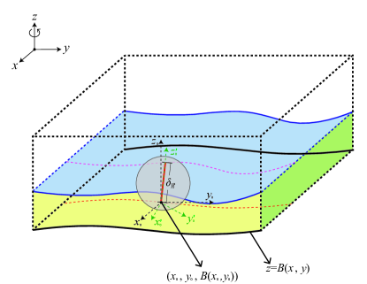
Figure 1: Size at a point $(x_{0},y_{0},B(x_{0},y_{0}))$ of the bottom boundary.

Thus, the boundary layer size is considered below on a localized area, where $\theta$ and $\phi$ are regarded as constants. Firstly, from (11), we obtain

$$\frac{\partial(x^{\prime},y^{\prime},z^{\prime})}{\partial(x,y,z)}=\begin{pmatrix}\cos\theta&-\sin\theta\sin\phi&-\sin\theta\cos\phi\\ 0&\cos\phi&-\sin\phi\\ \sin\theta&\cos\theta\sin\phi&\cos\theta\cos\phi\end{pmatrix}=:\boldsymbol{R_{0}}^{-1}.$$

Then, the derivation operators can be expressed as

$$\nabla=\begin{pmatrix}\partial_{x}\\ \partial_{y}\\ \partial_{z}\end{pmatrix}=\frac{\partial(x^{\prime},y^{\prime},z^{\prime})}{\partial(x,y,z)}\begin{pmatrix}\partial_{{x}^{\prime}}\\ \partial_{{y}^{\prime}}\\ \partial_{{z}^{\prime}}\end{pmatrix}=:\boldsymbol{R_{0}}^{-1}\nabla^{\prime},$$

and $\Delta=\partial_{x}^{2}+\partial_{y}^{2}+\partial_{z}^{2}=(\partial_{x^{\prime}}^{2}+\partial_{y^{\prime}}^{2}+\partial_{z^{\prime}}^{2})=:\Delta^{\prime}$. The system in the new coordinates $(x^{\prime},y^{\prime},z^{\prime})$ has been obtained as

$$\begin{cases}\partial_{t}\tilde{\boldsymbol{u}}^{\varepsilon}-\nu\varepsilon\Delta^{\prime}\tilde{\boldsymbol{u}}^{\varepsilon}+\varepsilon^{-1}\widetilde{\boldsymbol{R}}\tilde{\boldsymbol{u}}^{\varepsilon}+\varepsilon^{-1}\nabla^{\prime}p^{\varepsilon}=0,\\ \nabla^{\prime}\cdot\tilde{\boldsymbol{u}}^{\varepsilon}=0,\end{cases}$$ (12)

where

$$\tilde{\boldsymbol{u}}^{\varepsilon}:=\boldsymbol{R_{0}}\boldsymbol{u}^{\varepsilon},$$

and

$$\widetilde{\boldsymbol{R}}:= \begin{pmatrix}0&-\cos\theta\cos\phi&\cos\theta\sin\phi\\ \cos\theta\cos\phi&0&-\sin\theta\\ -\cos\theta\sin\phi&\sin\theta&0\end{pmatrix}.$$

2.2 Calculate the size of the boundary layer

In the following, we use the method described in literature [9] to calculate the size of the boundary layer. Firstly, making a Laplace-Fourier analysis for (12), we have

$$\begin{pmatrix}i\tau+\nu\varepsilon{|\xi|}^{2}&\quad-\varepsilon^{-1}\cos\theta\cos\phi&\quad\varepsilon^{-1}\cos\theta\sin\phi&\quad\varepsilon^{-1}i\xi_{1}\\ \varepsilon^{-1}\cos\theta\cos\phi&\quad i\tau+\nu\varepsilon{|\xi|}^{2}&\quad-\varepsilon^{-1}\sin\theta&\quad\varepsilon^{-1}i\xi_{2}\\ -\varepsilon^{-1}\cos\theta\sin\phi&\quad\varepsilon^{-1}\sin\theta&\quad i\tau+\nu\varepsilon{|\xi|}^{2}&\quad\varepsilon^{-1}i\xi_{3}\\ i\xi_{1}&\quad i\xi_{2}&\quad i\xi_{3}&\quad 0\end{pmatrix}\begin{pmatrix}\hat{\tilde{u}}^{\varepsilon}_{1}\\ \hat{\tilde{u}}^{\varepsilon}_{2}\\ \hat{\tilde{u}}^{\varepsilon}_{3}\\ \hat{p}^{\varepsilon}\end{pmatrix}=0.$$

Figure 2: Size of the boundary layer in the original coordinate system.

Recalling condition (8) guarantees that the top and bottom boundary layers are dominant. Then, the size of the bottom boundary along the normal direction is

$${\delta}_{\overrightarrow{n}}={\xi}_{3}^{-1}=\sqrt{\nu}\varepsilon\cos^{-\frac{1}{2}}\gamma.$$

For the following analysis, we first transfer the size of the boundary layer to the original coordinate system, mainly because we aim to utilize the structure of the equation (5).

As depicted in Figure 2, the boundary layer size along the $z$-axis in the original coordinate system is

$${\delta}(x,y)=\frac{{\delta}_{\overrightarrow{n}}(x,y)}{\cos\gamma(x,y)}=\sqrt{\nu}\varepsilon\cos^{-\frac{3}{2}}\gamma(x,y).$$

Furthermore, both boundary layers are of equal size due to the parallel nature of their top and bottom boundaries.

3 The solution of the linear system

In the first step, we study the linearized equations

$$\begin{cases}\partial_{t}\boldsymbol{u}_{\mathrm{L}}^{\varepsilon}-\nu\varepsilon\Delta\boldsymbol{u}_{\mathrm{L}}^{\varepsilon}+\varepsilon^{-1}\boldsymbol{R}\boldsymbol{u}_{\mathrm{L}}^{\varepsilon}+\varepsilon^{-1}\nabla p^{\varepsilon}_{\mathrm{L}}=0,\\ \nabla\cdot\boldsymbol{u}_{\mathrm{L}}^{\varepsilon}=0,\\ \boldsymbol{u}_{\mathrm{L}}^{\varepsilon}|_{\partial\Omega}=0,\quad\boldsymbol{u}_{\mathrm{L}}^{\varepsilon}|_{t=0}=\boldsymbol{u}_{\mathrm{L}0}^{\varepsilon}.\end{cases}$$ (13)

The following, by using the analysis in Section 2, we construct the solution $(\boldsymbol{u}_{\mathrm{L}}^{\mathrm{b}},p_{\mathrm{L}}^{\mathrm{b}})$ in the vicinity of the bottom boundary in the following form:

$$\begin{cases}\boldsymbol{u}_{\mathrm{L}}^{\mathrm{b}}=\sum_{i=0}^{\infty}{\delta}^{i}\big{[}\boldsymbol{u}^{i,\mathrm{int,b}}(t,x,y,z)+\boldsymbol{u}^{i,\mathrm{BL,b}}(t,\tilde{x},\tilde{y},\tilde{z})\big{]},\\ p_{\mathrm{L}}^{\mathrm{b}}=\sum_{i=0}^{\infty}{\delta}^{i}\big{[}p^{i,\mathrm{int,b}}(t,x,y,z)+p^{i,\mathrm{BL,b}}(t,\tilde{x},\tilde{y},\tilde{z})\big{]},\end{cases}$$ (14)

where

$$(\tilde{x},\tilde{y},\tilde{z})=\Big{(}x,y,\tfrac{z-B(x,y)}{{\delta}(x,y)}\Big{)}.$$ (15)

Near the top boundary, we construct an approximate solution $(\boldsymbol{u}_{\mathrm{L}}^{\mathrm{t}},{p}_{\mathrm{L}}^{\mathrm{t}})$ of the form

$$\begin{cases}{\boldsymbol{u}}_{\mathrm{L}}^{\mathrm{t}}=\sum_{i=0}^{\infty}{\delta}^{i}\big{[}\boldsymbol{u}^{i,\mathrm{int,t}}(t,x,y,z)+\boldsymbol{u}^{i,\mathrm{BL,t}}(t,\bar{x},\bar{y},\bar{z})\big{]},\\ {p}_{\mathrm{L}}^{\mathrm{t}}=\sum_{i=0}^{\infty}{\delta}^{i}\big{[}p^{i,\mathrm{int,t}}(t,x,y,z)+p^{i,\mathrm{BL,t}}(t,\bar{x},\bar{y},\bar{z})\big{]},\end{cases}$$ (16)

where

$$(\bar{x},\bar{y},\bar{z})=\Big{(}x,y,\tfrac{2+B(x,y)-z}{{\delta}(x,y)}\Big{)}.$$ (17)

And we also put a nature boundary condition as

$$\lim\limits_{\delta\rightarrow 0^{+}}\boldsymbol{u}^{i,\mathrm{BL,b}}(t,\tilde{x},\tilde{y},\tilde{z})=\lim\limits_{\delta\rightarrow 0^{+}}\boldsymbol{u}^{i,\mathrm{BL,t}}(t,\bar{x},\bar{y},\bar{z})=0.$$

Next, we decide the precise forms of (14) or (16) by analyzing the order of $\delta$.

3.1 The construction of $(\boldsymbol{u}_{\mathrm{L}}^{\mathrm{b}},p_{\mathrm{L}}^{\mathrm{b}})$

The following analysis includes the bottom boundary approximation in the linear approximation equations and examines the main components of the interior and boundary terms. Before being substituted into the approximate equations, the derivatives of the boundary layer term under the new coordinate system $(\tilde{x},\tilde{y},\tilde{z})=(x,y,\frac{z-B}{\sqrt{\nu}\varepsilon}\cos^{\frac{3}{2}}\gamma)$ are computed and can be expressed as follows

$$\begin{pmatrix}\partial_{x}\\ \partial_{y}\\ \partial_{z}\end{pmatrix}=\begin{pmatrix}1&\quad 0&\quad\tilde{z}_{x}\\ 0&\quad 1&\quad\tilde{z}_{y}\\ 0&\quad 0&\quad\delta^{-1}\end{pmatrix}\begin{pmatrix}\partial_{\tilde{x}}\\ \partial_{\tilde{y}}\\ \partial_{\tilde{z}}\end{pmatrix},$$

where

$$\tilde{z}_{x}=-\tfrac{3\tilde{z}}{2}\tan\gamma\gamma_{x}-(\sqrt{\nu}\varepsilon)^{-1}\cos^{\frac{3}{2}}\gamma B_{x},\quad\tilde{z}_{y}=-\tfrac{3\tilde{z}}{2}\tan\gamma\gamma_{y}-(\sqrt{\nu}\varepsilon)^{-1}\cos^{\frac{3}{2}}\gamma B_{y}.$$

Next, we substitute the approximate forms of (14) or (16) for the top and bottom boundaries into the linear system (13) and analyze its $\delta^{i}$-order parts ($i=-2,-1,0,\cdots$).

3.1.1 The $\mathcal{O}(\delta^{-2})$-order part in the system.

We obtain the highest order term as $\delta^{-2}$ upon simple computation

$$\partial_{\tilde{z}}p^{0,\mathrm{BL,b}}=0.$$

It is natural to take $p^{0,\mathrm{BL,b}}=0$, implying that the highest order pressure term is vanishing in the boundary layer.

3.1.2 The $\mathcal{O}(\delta^{-1})$-order part in the system.

From the $\delta^{-1}$-order internal term, we get

$$\begin{cases}-\boldsymbol{E_{1}}\boldsymbol{u}_{h}^{0,\mathrm{int}}+\nabla_{h}p^{0,\mathrm{int}}=0,\\ \partial_{z}p^{0,\mathrm{int}}=0,\end{cases}$$ (18)

and the incompressible condition $\nabla\cdot\boldsymbol{u}^{0,\mathrm{int}}=0$, it is evident that $p^{0,\mathrm{int}}$ and $\boldsymbol{u}^{0,\mathrm{int}}$ are independent of $z$. Moreover, we have

$$p^{0,\mathrm{int}}=\Delta_{h}^{-1}\nabla^{\perp}_{h}\cdot\boldsymbol{u}_{h}^{0,\mathrm{int}}.$$ (19)

Similarly, we take the $\delta^{-1}$-order bottom boundary terms from the equations as

$$\begin{cases}\cos\gamma\partial_{\tilde{z}}^{2}u_{1}^{0,\mathrm{BL,b}}+u_{2}^{0,\mathrm{BL,b}}+B_{x}\partial_{\tilde{z}}p^{1,\mathrm{BL,b}}=0,\\ \cos\gamma\partial_{\tilde{z}}^{2}u_{2}^{0,\mathrm{BL,b}}-u_{1}^{0,\mathrm{BL,b}}+B_{y}\partial_{\tilde{z}}p^{1,\mathrm{BL,b}}=0,\\ \partial_{\tilde{z}}p^{1,\mathrm{BL,b}}=\cos\gamma\partial_{\tilde{z}}^{2}u_{3}^{0,\mathrm{BL,b}},\\ \partial_{\tilde{z}}u_{3}^{0,\mathrm{BL,b}}=\nabla_{h}B\cdot\partial_{\tilde{z}}\boldsymbol{u}_{h}^{0,\mathrm{BL,b}}.\end{cases}$$ (20)

Substituting $\eqref{3.11}_{3}$ into $\eqref{3.11}_{1,2}$, and combining $\eqref{3.11}_{4}$ gives

$$\boldsymbol{H_{0}}\partial_{\tilde{z}}^{2}\boldsymbol{u}_{h}^{0,\mathrm{BL,b}}+\cos^{-1}\gamma\boldsymbol{E_{1}}\boldsymbol{u}_{h}^{0,\mathrm{BL,b}}=0.$$

Recalling that $\boldsymbol{u}_{h}^{0,\mathrm{int}}(t,x,y)$ is independent on ${z}$, under the boundary conditions

$$\boldsymbol{u}^{0,\mathrm{BL,b}}(t,\tilde{x},\tilde{y},\tilde{z})|_{\tilde{z}=0}=-\boldsymbol{u}^{0,\mathrm{int}}(t,x,y),\quad\lim_{\tilde{z}\rightarrow\infty}\boldsymbol{u}^{0,\mathrm{BL,b}}(t,\tilde{x},\tilde{y},\tilde{z})=0,$$ (21)

we conclude that

$$\boldsymbol{u}_{h}^{0,\mathrm{BL,b}}=-\mathrm{e}^{-\frac{\tilde{z}}{\sqrt{2}}}\Big{(}\cos\tfrac{\tilde{z}}{\sqrt{2}}\boldsymbol{E}+\sin\tfrac{\tilde{z}}{\sqrt{2}}\cos\gamma\boldsymbol{E_{1}}\boldsymbol{H_{0}}\Big{)}\boldsymbol{u}_{h}^{0,\mathrm{int}}.$$ (22)

From $\eqref{3.11}_{4}$, we have

$$\partial_{\tilde{z}}u_{3}^{0,\mathrm{BL,b}}=\mathrm{e}^{-\frac{\tilde{z}}{\sqrt{2}}}\Big{(}\sin(\tfrac{\tilde{z}}{\sqrt{2}}+\tfrac{\pi}{4})\nabla_{h}B+\sin(\tfrac{\tilde{z}}{\sqrt{2}}-\tfrac{\pi}{4})\cos\gamma\cdot\nabla^{\perp}_{h}B\Big{)}\cdot\boldsymbol{u}_{h}^{0,\mathrm{int}}.$$ (23)

Due to (21), integrating (23) from $\tilde{z}$ to $+\infty$, we obtain

$$u_{3}^{0,\mathrm{BL,b}}=-\mathrm{e}^{-\frac{\tilde{z}}{\sqrt{2}}}\Big{(}\cos\tfrac{\tilde{z}}{\sqrt{2}}\nabla_{h}B+\sin\tfrac{\tilde{z}}{\sqrt{2}}\cos\gamma\nabla^{\perp}_{h}B\Big{)}\cdot\boldsymbol{u}_{h}^{0,\mathrm{int}}.$$ (24)

Combining (24) with $\eqref{3.11}_{3}$ yields

$$p^{1,\mathrm{BL,b}}=\mathrm{e}^{-\frac{\tilde{z}}{\sqrt{2}}}\Big{(}\sin(\tfrac{\tilde{z}}{\sqrt{2}}+\tfrac{\pi}{4})\cos\gamma\nabla_{h}B+\sin(\tfrac{\tilde{z}}{\sqrt{2}}-\tfrac{\pi}{4})\cos^{2}\gamma\nabla^{\perp}_{h}B\Big{)}\cdot\boldsymbol{u}_{h}^{0,\mathrm{int}}.$$ (25)

Based on the boundary condition $u_{3}^{0,\mathrm{BL,b}}|_{\tilde{z}=0}=-u_{3}^{0,\mathrm{int}}|_{z=B}$, and then combining (24) with the incompressible condition $\nabla\cdot\boldsymbol{u}^{0,\mathrm{int}}=0$, we conclude that $u_{3}^{0,\mathrm{int}}$ is independent of ${z}$ and can be taken as

$$u_{3}^{0,\mathrm{int}}=\nabla_{h}B\cdot\boldsymbol{u}_{h}^{0,\mathrm{int}}.$$ (26)

Next, we need to determine the equation for $\boldsymbol{u}^{0,\mathrm{int}}_{h}(t,x,y)$.

3.1.3 The $\mathcal{O}(1)$-order part in the system.

Like the above analysis, we have the $\mathcal{O}(1)$-order boundary term in the form

$$\boldsymbol{H_{0}}\partial_{\tilde{z}}^{2}\boldsymbol{u}_{h}^{1,\mathrm{BL,b}}+\cos^{-1}\gamma\boldsymbol{E_{1}}\boldsymbol{u}_{h}^{1,\mathrm{BL,b}}=\begin{pmatrix}1&0&B_{x}\\ 0&1&B_{y}\end{pmatrix}\boldsymbol{\widetilde{D}}+\partial_{\tilde{z}}\widetilde{D}_{0}\nabla_{h}B,$$ (27)

where

$$\boldsymbol{\widetilde{D}}:= \tfrac{3}{2}\cos\gamma{\footnotesize\begin{pmatrix}\boldsymbol{H}\nabla_{h}B\\ 0\end{pmatrix}}(p^{1,\mathrm{BL,b}}-\tilde{z}\partial_{\tilde{z}}p^{1,\mathrm{BL,b}})$$

$$-\cos^{2}\gamma\Big{(}3\cos^{2}\gamma\nabla_{h}B^{T}\boldsymbol{H}\nabla_{h}B(\partial_{\tilde{z}}+\tilde{z}\partial^{2}_{\tilde{z}})-(\Delta_{h}B+2(\nabla_{h}B\cdot\nabla_{\tilde{h}}))\partial_{\tilde{z}}\Big{)}\boldsymbol{u}^{0,\mathrm{BL,b}}$$

$$+\sqrt{\tfrac{\cos\gamma}{\nu}}\partial_{t}\boldsymbol{u}^{0,\mathrm{BL,b}}+\cos^{-1}\gamma{\footnotesize\begin{pmatrix}\nabla_{\tilde{h}}\\ 0\end{pmatrix}}p^{1,\mathrm{BL,b}},$$

$$\widetilde{D}_{0}:= \nabla_{\tilde{h}}\cdot\boldsymbol{u}_{h}^{0,\mathrm{BL,b}}-\tfrac{3\tilde{z}}{2}\cos^{2}\gamma\boldsymbol{H}\nabla_{h}B\cdot\partial_{\tilde{z}}\boldsymbol{u}_{h}^{0,\mathrm{BL,b}},\quad\text{and}\quad\nabla_{\tilde{h}}:=(\partial_{\tilde{x}},\partial_{\tilde{y}}).$$

Then (27) can be rewritten as

$$\partial_{\tilde{z}}^{2}\boldsymbol{Q}^{-1}\boldsymbol{u}_{h}^{1,\mathrm{BL,b}}+\begin{pmatrix}i&0\\ 0&-i\end{pmatrix}\boldsymbol{Q}^{-1}\boldsymbol{u}_{h}^{1,\mathrm{BL,b}}$$ (28)

$$\quad=\boldsymbol{Q}^{-1}\boldsymbol{H_{0}}^{-1}\bigg{(}\begin{pmatrix}1&0&B_{x}\\ 0&1&B_{y}\end{pmatrix}\boldsymbol{\widetilde{D}}+\partial_{\tilde{z}}\widetilde{D}_{0}\nabla_{h}B\bigg{)}=:\begin{pmatrix}\widetilde{G}_{1}\\ \widetilde{G}_{2}\end{pmatrix},$$

where

$$\boldsymbol{Q}:=\begin{pmatrix}\cos\gamma(1+B_{y}^{2})&\cos\gamma(1+B_{y}^{2})\\ i-\cos\gamma B_{x}B_{y}&-i-\cos\gamma B_{x}B_{y}\end{pmatrix},$$ (29)

and

$$\boldsymbol{Q}^{-1}:=-i\big{(}2\cos\gamma(1+B_{y}^{2})\big{)}^{-1}\begin{pmatrix}i+\cos\gamma B_{x}B_{y}&\cos\gamma(1+B_{y}^{2})\\ i-\cos\gamma B_{x}B_{y}&-\cos\gamma(1+B_{y}^{2})\end{pmatrix}.$$ (30)

Solving equations (28) with the boundary conditions

$$\boldsymbol{u}_{h}^{1,\mathrm{BL,b}}(t,\tilde{x},\tilde{y},\tilde{z})|_{\tilde{z}=0}=-\boldsymbol{u}_{h}^{1,\mathrm{int,b}}(t,x,y,z)|_{z=B},\quad\lim_{\tilde{z}\rightarrow\infty}\boldsymbol{u}_{h}^{1,\mathrm{BL,b}}(t,\tilde{x},\tilde{y},\tilde{z})=0,$$

yields

$$\boldsymbol{u}_{h}^{1,\mathrm{BL,b}}= -\mathrm{e}^{-\frac{\tilde{z}}{\sqrt{2}}}\Big{(}\cos\tfrac{\tilde{z}}{\sqrt{2}}\boldsymbol{E}+\sin\tfrac{\tilde{z}}{\sqrt{2}}\cos\gamma\boldsymbol{E_{1}}\boldsymbol{H_{0}}\Big{)}\boldsymbol{u}_{h}^{1,\mathrm{int,b}}|_{z=B}$$ (31)

$$+\boldsymbol{Q}\begin{pmatrix}\int_{0}^{\tilde{z}}{\mathrm{e}}^{-\sqrt{i}(\tilde{z}-\tau)}\widetilde{G}_{1}(\tau)\,{d}\tau\\[3.0pt] \int_{0}^{\tilde{z}}{\mathrm{e}}^{-\sqrt{-i}(\tilde{z}-\tau)}\widetilde{G}_{2}(\tau)\,{d}\tau\end{pmatrix}.$$

Next, according to the incompressible condition, one has

$$\partial_{\tilde{z}}u_{3}^{1,\mathrm{BL,b}}=\nabla_{h}B\cdot\partial_{\tilde{z}}\boldsymbol{u}_{h}^{1,\mathrm{BL,b}}-\nabla_{\tilde{h}}\cdot\boldsymbol{u}_{h}^{0,\mathrm{BL,b}}+\tfrac{3\tilde{z}}{2}\cos^{2}\gamma\boldsymbol{H}\nabla_{h}B\cdot\partial_{\tilde{z}}\boldsymbol{u}_{h}^{0,\mathrm{BL,b}}.$$ (32)

From the equation about $u_{3}^{1,\mathrm{BL,b}}$ in the $\mathcal{O}(1)$-order term of the boundary layer, it follows that

$$\partial_{\tilde{z}}p^{2,\mathrm{BL,b}}$$ (33)

$$=\cos\gamma\partial^{2}_{\tilde{z}}u_{3}^{1,\mathrm{BL,b}}-\cos^{\frac{3}{2}}\gamma\nu^{-\frac{1}{2}}\partial_{t}u_{3}^{0,\mathrm{BL,b}}$$

$$\quad+\cos^{3}\gamma\Big{(}3\cos^{2}\gamma\nabla_{h}B^{T}\boldsymbol{H}\nabla_{h}B(\partial_{\tilde{z}}+\tilde{z}\partial^{2}_{\tilde{z}})-(\Delta_{h}B+2(\nabla_{h}B\cdot\nabla_{\tilde{h}}))\partial_{\tilde{z}}\Big{)}u_{3}^{0,\mathrm{BL,b}}.$$

Since we already have the forms of $\boldsymbol{u}^{0,\mathrm{BL,b}}$, $\boldsymbol{u}_{h}^{1,\mathrm{BL,b}}$ and ${p}^{1,\mathrm{BL,b}}$, combining (32)-(33), we get the form of $u_{3}^{1,\mathrm{BL,b}}$ as

$$u_{3}^{1,\mathrm{BL,b}}(t,\tilde{x},\tilde{y},\tilde{z})$$ (34)

$$=\int_{\tilde{z}}^{+\infty}\Big{(}-\nabla_{h}B\cdot\partial_{\tilde{z}}\boldsymbol{u}_{h}^{1,\mathrm{BL,b}}+\nabla_{\tilde{h}}\cdot\boldsymbol{u}_{h}^{0,\mathrm{BL,b}}-\tfrac{3\tilde{z}}{2}\cos^{2}\gamma\boldsymbol{H}\nabla_{h}B\cdot\partial_{\tilde{z}}\boldsymbol{u}_{h}^{0,\mathrm{BL,b}}\Big{)}\,d\tilde{z},$$

and $p^{2,\mathrm{BL,b}}$ as

$$p^{2,\mathrm{BL,b}}(t,\tilde{x},\tilde{y},\tilde{z})$$ (35)

$$=\int_{\tilde{z}}^{+\infty}\Big{(}-\cos\gamma\partial^{2}_{\tilde{z}}u_{3}^{1,\mathrm{BL,b}}+\cos^{\frac{3}{2}}\gamma\nu^{-\frac{1}{2}}\partial_{t}u_{3}^{0,\mathrm{BL,b}}$$

$$\quad-\cos^{3}\gamma\big{(}3\cos^{2}\gamma\nabla_{h}B^{T}\boldsymbol{H}\nabla_{h}B(\partial_{\tilde{z}}+\tilde{z}\partial^{2}_{\tilde{z}})-(\Delta_{h}B+2(\nabla_{h}B\cdot\nabla_{\tilde{h}}))\partial_{\tilde{z}}\big{)}u_{3}^{0,\mathrm{BL,b}}\Big{)}\,d\tilde{z}.$$

Now, let’s turn to the $\mathcal{O}(1)$-order part from the interior, there holds

$$\begin{cases}\partial_{t}\boldsymbol{u}_{h}^{0,\mathrm{int}}-\sqrt{\nu}\cos^{-\frac{3}{2}}\gamma\boldsymbol{E_{1}}\boldsymbol{u}_{h}^{1,\mathrm{int}}+\nabla_{h}(\sqrt{\nu}\cos^{-\frac{3}{2}}\gamma p^{1,\mathrm{int}})=0,\\ \nabla_{h}\cdot\boldsymbol{u}_{h}^{0,\mathrm{int}}=0.\end{cases}$$ (36)

In analyzing the subsequent limit system, understanding the composition of $\boldsymbol{u}^{1,\mathrm{int}}=(\boldsymbol{u}_{h}^{1,\mathrm{int}},u_{3}^{1,\mathrm{int}})$ in system (36) is essential. In the flat case, $\boldsymbol{u}^{1,\mathrm{int}}$ is determined by $\boldsymbol{u}_{h}^{0,\mathrm{int}}$, while in the non-flat domain, the boundary’s geometry affects the form and construction of $\boldsymbol{u}^{1,\mathrm{int}}$, adding complexity to the process.

Initially, by considering the boundary condition of $u_{3}^{1,\mathrm{BL,b}}$, we derive

$$u_{3}^{1,\mathrm{int}}(t,x,y,{z})|_{z=B}$$ (37)

$$=\tfrac{1}{2\sqrt{2}}\cos^{2}\gamma\nabla_{h}B^{T}\boldsymbol{H}(3\boldsymbol{E}+\cos\gamma\boldsymbol{E_{1}}\boldsymbol{H_{0}})\boldsymbol{u}_{h}^{0,\mathrm{int}}-\tfrac{1}{\sqrt{2}}\cos\gamma\nabla_{h}B^{T}\boldsymbol{E_{1}}\boldsymbol{H}\boldsymbol{u}_{h}^{0,\mathrm{int}}$$

$$\quad-\tfrac{1}{\sqrt{2}}\cos\gamma\Big{(}\nabla_{h}B(\nabla^{\perp}_{h}B\cdot\nabla_{h})-\nabla_{h}^{\bot}\Big{)}\cdot\boldsymbol{u}_{h}^{0,\mathrm{int}}+\nabla_{h}B^{T}\boldsymbol{u}_{h}^{1,\mathrm{int}}(t,x,y,{z})|_{z=B}.$$

Given $\boldsymbol{u}^{1,\mathrm{int}}$ satisfies the incompressibility condition

$$\partial_{z}u_{3}^{1,\mathrm{int}}=-\nabla_{h}\cdot\boldsymbol{u}_{h}^{1,\mathrm{int}}-\tfrac{3\cos^{2}\gamma}{2}\nabla_{h}B^{T}\boldsymbol{H}\boldsymbol{u}_{h}^{1,\mathrm{int}},$$

and $\boldsymbol{u}_{h}^{1,\mathrm{int}}$ describes an internal structure between two parallel plates, we take it independency on $z$, leading to

$$u_{3}^{1,\mathrm{int}}(t,x,y,z)=(B+1-z)\big{(}\nabla_{h}\cdot\boldsymbol{u}_{h}^{1,\mathrm{int}}+\tfrac{3\cos^{2}\gamma}{2}\nabla_{h}B^{T}\boldsymbol{H}\boldsymbol{u}_{h}^{1,\mathrm{int}}\big{)}+\nabla_{h}B^{T}\boldsymbol{u}_{h}^{1,\mathrm{int}}(t,x,y).$$ (38)

Below, based on (37) and (38), we analyze the constitution of $\boldsymbol{u}_{h}^{1,\mathrm{int}}$. Firstly, through direct calculation, we obtain

$$\tfrac{\cos\gamma}{\sqrt{2}}\nabla_{h}^{\bot}\cdot\boldsymbol{u}_{h}^{0,\mathrm{int}}+\tfrac{\cos^{3}\gamma}{2\sqrt{2}}\nabla_{h}B^{T}\boldsymbol{H}\boldsymbol{E_{1}}\boldsymbol{u}_{h}^{0,\mathrm{int}}+\tfrac{3\cos^{2}\gamma}{2\sqrt{2}}\nabla_{h}B^{T}\boldsymbol{H}\boldsymbol{u}_{h}^{0,\mathrm{int}}$$

$$= \nabla_{h}\cdot\big{(}\tfrac{\cos\gamma}{\sqrt{2}}\boldsymbol{E_{1}}\boldsymbol{u}_{h}^{0,\mathrm{int}}+\tfrac{1}{\sqrt{2}}\boldsymbol{u}_{h}^{0,\mathrm{int}}\big{)}+\tfrac{3\cos^{2}\gamma}{2}\nabla_{h}B^{T}\boldsymbol{H}\big{(}\tfrac{\cos\gamma}{\sqrt{2}}\boldsymbol{E_{1}}\boldsymbol{u}_{h}^{0,\mathrm{int}}+\tfrac{1}{\sqrt{2}}\boldsymbol{u}_{h}^{0,\mathrm{int}}\big{)},$$

where $\tfrac{\cos\gamma}{\sqrt{2}}\boldsymbol{E_{1}}\boldsymbol{u}_{h}^{0,\mathrm{int}}+\tfrac{1}{\sqrt{2}}\boldsymbol{u}_{h}^{0,\mathrm{int}}$ represents the part of $\boldsymbol{u}_{h}^{1,\mathrm{int}}$ corresponding to the flat boundary case.

Given

$$\tfrac{\cos^{3}\gamma}{2\sqrt{2}}\nabla_{h}B^{T}\boldsymbol{H}\boldsymbol{E_{1}}(\nabla_{h}B\otimes\nabla_{h}B)\boldsymbol{u}_{h}^{0,\mathrm{int}}-\tfrac{\cos\gamma}{\sqrt{2}}\nabla_{h}B^{T}\boldsymbol{E_{1}}\boldsymbol{H}\boldsymbol{u}_{h}^{0,\mathrm{int}}-\tfrac{\cos\gamma}{\sqrt{2}}\nabla_{h}B^{T}(\nabla^{\bot}_{h}B\cdot\nabla_{h})\boldsymbol{u}_{h}^{0,\mathrm{int}}$$

$$= \nabla_{h}\cdot\big{(}\tfrac{\cos\gamma}{\sqrt{2}}\boldsymbol{E_{1}}(\nabla_{h}B\otimes\nabla_{h}B)\boldsymbol{u}_{h}^{0,\mathrm{int}}\big{)}+\tfrac{3\cos^{2}\gamma}{2}\nabla_{h}B^{T}\boldsymbol{H}\big{(}\tfrac{\cos\gamma}{\sqrt{2}}\boldsymbol{E_{1}}(\nabla_{h}B\otimes\nabla_{h}B)\boldsymbol{u}_{h}^{0,\mathrm{int}}\big{)},$$

we conclude that $\tfrac{\cos\gamma}{\sqrt{2}}\boldsymbol{E_{1}}(\nabla_{h}B\otimes\nabla_{h}B)\boldsymbol{u}_{h}^{0,\mathrm{int}}$ represents the portion of $\boldsymbol{u}_{h}^{1,\mathrm{int}}$ subjected to geometric constraints.

Thus, we have $\boldsymbol{u}_{h}^{1,\mathrm{int}}$ and $u_{3}^{1,\mathrm{int}}$ represented as

$$\boldsymbol{u}_{h}^{1,\mathrm{int}}(t,x,y)=\tfrac{\cos\gamma}{\sqrt{2}}\boldsymbol{E_{1}}\boldsymbol{H_{0}}\boldsymbol{u}_{h}^{0,\mathrm{int}}+\tfrac{1}{\sqrt{2}}\boldsymbol{u}_{h}^{0,\mathrm{int}},$$ (39)

and

$$u_{3}^{1,\mathrm{int}}(t,x,y,z)$$ (40)

$$=\tfrac{1}{\sqrt{2}}(B+1-z)\nabla_{h}\cdot\big{(}\cos\gamma\boldsymbol{E_{1}}\boldsymbol{H_{0}}\boldsymbol{u}_{h}^{0,\mathrm{int}}\big{)}$$

$$\quad+(B+1-z)\tfrac{3\cos^{2}\gamma}{2\sqrt{2}}\nabla_{h}B^{T}\boldsymbol{H}\big{(}\cos\gamma\boldsymbol{E_{1}}\boldsymbol{H_{0}}+\boldsymbol{E}\big{)}\boldsymbol{u}_{h}^{0,\mathrm{int}}+\tfrac{1}{\sqrt{2}}\nabla_{h}B^{T}\big{(}\cos\gamma\boldsymbol{E_{1}}\boldsymbol{H_{0}}+\boldsymbol{E}\big{)}\boldsymbol{u}_{h}^{0,\mathrm{int}}.$$

Under the form of (39), we get the equations for ${\boldsymbol{u}}_{h}^{0,\mathrm{int}}$ as

$$\begin{cases}\partial_{t}{\boldsymbol{u}}_{h}^{0,\mathrm{int}}+\sqrt{\frac{\nu}{2\cos\gamma}}(\boldsymbol{H_{0}}-\cos^{-1}\gamma\boldsymbol{E_{1}})\boldsymbol{u}_{h}^{0,\mathrm{int}}+\nabla_{h}(\sqrt{\nu}\cos^{-\frac{3}{2}}\gamma p^{1,\mathrm{int}})=0,\\ \nabla_{h}\cdot{\boldsymbol{u}}_{h}^{0,\mathrm{int}}=0.\end{cases}$$ (41)

3.1.4 The $o(\delta)$-order part in the system.

Since the terms $\boldsymbol{u}^{2,\mathrm{BL,b}}$ and $\boldsymbol{u}^{2,\mathrm{int,b}}$ are of $o(\delta)$, which only affect the incompressible condition. Specifically, when considering the term of $\delta^{1}$-order from the incompressible condition, the following holds

$$\partial_{\tilde{z}}u_{3}^{2,\mathrm{BL,b}}= \nabla_{h}B\cdot\partial_{\tilde{z}}\boldsymbol{u}_{h}^{2,\mathrm{BL,b}}-\big{(}\tfrac{3\cos^{2}\gamma}{2}\boldsymbol{H}\nabla_{h}B+\nabla_{\tilde{h}}\big{)}\cdot\boldsymbol{u}_{h}^{1,\mathrm{BL,b}}$$ (42)

$$+\tfrac{3\tilde{z}\cos^{2}\gamma}{2}\nabla_{h}B^{T}\boldsymbol{H}\partial_{\tilde{z}}\boldsymbol{u}_{h}^{1,\mathrm{BL,b}}.$$

Therefore, for $\boldsymbol{u}^{2,\mathrm{BL,b}}$, we take

$$u_{1}^{2,\mathrm{BL,b}}=u_{2}^{2,\mathrm{BL,b}}=0.$$ (43)

And then from (42), we get

$$\partial_{\tilde{z}}u_{3}^{2,\mathrm{BL,b}}= -\big{(}\tfrac{3\cos^{2}\gamma}{2}\boldsymbol{H}\nabla_{h}B+\nabla_{\tilde{h}}\big{)}\cdot\boldsymbol{u}_{h}^{1,\mathrm{BL,b}}+\tfrac{3\tilde{z}\cos^{2}\gamma}{2}\nabla_{h}B^{T}\boldsymbol{H}\partial_{\tilde{z}}\boldsymbol{u}_{h}^{1,\mathrm{BL,b}}.$$ (44)

By the form of $\boldsymbol{u}_{h}^{1,\mathrm{BL,b}}$ and (42), we get

$$u_{3}^{2,\mathrm{BL,b}}(t,\tilde{x},\tilde{y},\tilde{z})$$ (45)

$$=\int_{\tilde{z}}^{+\infty}\Big{(}\big{(}\tfrac{3\cos^{2}\gamma}{2}\boldsymbol{H}\nabla_{h}B+\nabla_{\tilde{h}}\big{)}\cdot\boldsymbol{u}_{h}^{1,\mathrm{BL,b}}-\tfrac{3\tilde{z}\cos^{2}\gamma}{2}\nabla_{h}B^{T}\boldsymbol{H}\partial_{\tilde{z}}\boldsymbol{u}_{h}^{1,\mathrm{BL,b}}\Big{)}\,d\tilde{z}.$$

Then, under the boundary condition

$$\boldsymbol{u}^{2,\mathrm{BL,b}}(t,\tilde{x},\tilde{y},\tilde{z})|_{\tilde{z}=0}=-\boldsymbol{u}^{2,\mathrm{int,b}}(t,x,y,z)|_{z=B},$$

we get

$$u_{1}^{2,\mathrm{int,b}}=u_{2}^{2,\mathrm{int,b}}=0,$$ (46)

and

$$u_{3}^{2,\mathrm{int,b}}(t,x,y)$$ (47)

$$=-\int_{0}^{+\infty}\Big{(}\big{(}\tfrac{3\cos^{2}\gamma}{2}\boldsymbol{H}\nabla_{h}B+\nabla_{\tilde{h}}\big{)}\cdot\boldsymbol{u}_{h}^{1,\mathrm{BL,b}}-\tfrac{3\tilde{z}\cos^{2}\gamma}{2}\nabla_{h}B^{T}\boldsymbol{H}\partial_{\tilde{z}}\boldsymbol{u}_{h}^{1,\mathrm{BL,b}}\Big{)}\,d\tilde{z}.$$

It is apparently $\boldsymbol{u}^{2,\mathrm{int,b}}=(u_{1}^{2,\mathrm{int,b}},u_{2}^{2,\mathrm{int,b}},u_{3}^{2,\mathrm{int,b}})$ satisfies the incompressible condition.

Combining the above analysis, we construct an approximate solution using only the bottom boundary information

$$\begin{cases}\begin{aligned} \boldsymbol{u}_{\mathrm{L}}^{\mathrm{b}}=&\boldsymbol{u}^{0,\mathrm{int}}+\delta\boldsymbol{u}^{1,\mathrm{int}}+\delta^{2}\boldsymbol{u}^{2,\mathrm{int,b}}+\boldsymbol{u}^{0,\mathrm{BL,b}}(t,\tilde{x},\tilde{y},\tilde{z})\\ &+\delta\boldsymbol{u}^{1,\mathrm{BL,b}}(t,\tilde{x},\tilde{y},\tilde{z})+\delta^{2}\boldsymbol{u}^{2,\mathrm{BL,b}}(t,\tilde{x},\tilde{y},\tilde{z}),\\ p_{\mathrm{L}}^{\mathrm{b}}=&p^{0,\mathrm{int}}+\delta p^{1,\mathrm{int}}+\delta p^{1,\mathrm{BL,b}}(t,\tilde{x},\tilde{y},\tilde{z})+\delta^{2}p^{2,\mathrm{BL,b}}(t,\tilde{x},\tilde{y},\tilde{z}),\end{aligned}\end{cases}$$ (48)

where $(\tilde{x},\tilde{y},\tilde{z})$ is determined by (15), $(\boldsymbol{u}_{h}^{0,\mathrm{int}},\delta p^{1,\mathrm{int}})$ is governed by (41), and the remaining terms can all be determined by $\boldsymbol{u}_{h}^{0,\mathrm{int}}$ as shown in (19)-(47). Moreover, based on the construction process, we get

$$\boldsymbol{u}_{\mathrm{L}}^{\mathrm{b}}|_{z=B(x,y)}=0\quad\mbox{and }\quad\nabla\cdot\boldsymbol{u}_{\mathrm{L}}^{\mathrm{b}}=0.$$

3.2 The construction of $(\boldsymbol{u}_{\mathrm{L}}^{\mathrm{t}},p_{\mathrm{L}}^{\mathrm{t}})$

Since the top and bottom boundaries are parallel, the treatment of approximate solutions near the top boundary is similar to that of the bottom boundary. It is straightforward to give an approximate solution $(\boldsymbol{u}_{\mathrm{L}}^{\mathrm{t}},p_{\mathrm{L}}^{\mathrm{t}})$ of the form:

$$\begin{cases}\begin{aligned} \boldsymbol{u}_{\mathrm{L}}^{\mathrm{t}}=&\boldsymbol{u}^{0,\mathrm{int}}+\delta\boldsymbol{u}^{1,\mathrm{int}}+\delta^{2}\boldsymbol{u}^{2,\mathrm{int,t}}+\boldsymbol{u}^{0,\mathrm{BL,t}}(t,\bar{x},\bar{y},\bar{z})\\ &+\delta\boldsymbol{u}^{1,\mathrm{BL,t}}(t,\bar{x},\bar{y},\bar{z})+\delta^{2}\boldsymbol{u}^{2,\mathrm{BL,t}}(t,\bar{x},\bar{y},\bar{z}),\\ p_{\mathrm{L}}^{\mathrm{t}}=&p^{0,\mathrm{int}}+\delta p^{1,\mathrm{int}}+\delta p^{1,\mathrm{BL,t}}(t,\bar{x},\bar{y},\bar{z})+\delta^{2}p^{2,\mathrm{BL,t}}(t,\bar{x},\bar{y},\bar{z}),\end{aligned}\end{cases}$$ (49)

where $(\bar{x},\bar{y},\bar{z})$ is determined by (17).

$(\boldsymbol{u}^{0,\mathrm{int}},\delta p^{1,\mathrm{int}})$, $p^{0,\mathrm{int}}$, and $\boldsymbol{u}^{1,\mathrm{int}}$ are still determined by (41), (26), (19) and (39)-(40), as well as $\boldsymbol{u}_{h}^{2,\mathrm{BL,t}}=\boldsymbol{u}_{h}^{2,\mathrm{int,t}}=0$.

The difference between the top and bottom boundary layers is due to the difference in the third variable: $\bar{z}=\tfrac{2+B(x,y)-z}{{\delta}(x,y)}$ and $\tilde{z}=\tfrac{z-B(x,y)}{{\delta}(x,y)}$. The other terms can therefore be expressed as

$$\boldsymbol{u}^{0,\mathrm{BL,t}}(t,\bar{x},\bar{y},\bar{z})=\begin{pmatrix}-\mathrm{e}^{-\frac{\bar{z}}{\sqrt{2}}}\big{(}\cos\tfrac{\bar{z}}{\sqrt{2}}\boldsymbol{E}+\sin\tfrac{\bar{z}}{\sqrt{2}}\cos\gamma\boldsymbol{E_{1}}\boldsymbol{H_{0}}\big{)}\boldsymbol{u}_{h}^{0,\mathrm{int}}\\ -\mathrm{e}^{-\frac{\bar{z}}{\sqrt{2}}}\big{(}\cos\tfrac{\bar{z}}{\sqrt{2}}\nabla_{h}B+\sin\tfrac{\bar{z}}{\sqrt{2}}\cos\gamma\nabla^{\perp}_{h}B\big{)}\cdot\boldsymbol{u}_{h}^{0,\mathrm{int}}\end{pmatrix},$$ (50)

$$p^{1,\mathrm{BL,t}}(t,\bar{x},\bar{y},\bar{z})$$ (51)

$$=-\mathrm{e}^{-\frac{\bar{z}}{\sqrt{2}}}\Big{(}\sin(\tfrac{\bar{z}}{\sqrt{2}}+\tfrac{\pi}{4})\cos\gamma\nabla_{h}B+\sin(\tfrac{\bar{z}}{\sqrt{2}}-\tfrac{\pi}{4})\cos^{2}\gamma\nabla^{\perp}_{h}B\Big{)}\cdot\boldsymbol{u}_{h}^{0,\mathrm{int}},$$

$$u_{3}^{1,\mathrm{BL,t}}(t,\bar{x},\bar{y},\bar{z})$$ (52)

$$=\int_{\bar{z}}^{+\infty}\Big{(}\tfrac{3\bar{z}}{2}\cos^{2}\gamma\boldsymbol{H}\nabla_{h}B\cdot\partial_{\bar{z}}\boldsymbol{u}_{h}^{0,\mathrm{BL,t}}-\nabla_{h}B\cdot\partial_{\bar{z}}\boldsymbol{u}_{h}^{1,\mathrm{BL,t}}-\nabla_{\bar{h}}\cdot\boldsymbol{u}_{h}^{0,\mathrm{BL,t}}\Big{)}\,d\bar{z},$$

$$p^{2,\mathrm{BL,t}}(t,\bar{x},\bar{y},\bar{z})=\int_{\bar{z}}^{+\infty}\Big{(}\cos\gamma\partial^{2}_{\bar{z}}u_{3}^{1,\mathrm{BL,t}}-\cos^{\frac{3}{2}}\gamma\nu^{-\frac{1}{2}}\partial_{t}u_{3}^{0,\mathrm{BL,t}}$$ (53)

$$\quad+\cos^{3}\gamma\Big{(}3\cos^{2}\gamma\nabla_{h}B^{T}\boldsymbol{H}\nabla_{h}B(\partial_{\bar{z}}+\bar{z}\partial^{2}_{\bar{z}})-(\Delta_{h}B+2(\nabla_{h}B\cdot\nabla_{\bar{h}}))\partial_{\bar{z}}\Big{)}u_{3}^{0,\mathrm{BL,t}}\Big{)}\,d\bar{z},$$

$$u_{3}^{2,\mathrm{BL,t}}(t,\bar{x},\bar{y},\bar{z})$$ (54)

$$=\int_{\bar{z}}^{+\infty}\Big{(}\big{(}\tfrac{3\cos^{2}\gamma}{2}\boldsymbol{H}\nabla_{h}B+\nabla_{\bar{h}}\big{)}\cdot\boldsymbol{u}_{h}^{1,\mathrm{BL,t}}+\tfrac{3\bar{z}\cos^{2}\gamma}{2}\nabla_{h}B^{T}\boldsymbol{H}\partial_{\bar{z}}\boldsymbol{u}_{h}^{1,\mathrm{BL,t}}\Big{)}\,d\bar{z},$$

$$u_{3}^{2,\mathrm{int,t}}(t,x,y)$$ (55)

$$=\int_{0}^{+\infty}\Big{(}\big{(}\tfrac{3\cos^{2}\gamma}{2}\boldsymbol{H}\nabla_{h}B+\nabla_{\bar{h}}\big{)}\cdot\boldsymbol{u}_{h}^{1,\mathrm{BL,t}}-\tfrac{3\bar{z}\cos^{2}\gamma}{2}\nabla_{h}B^{T}\boldsymbol{H}\partial_{\bar{z}}\boldsymbol{u}_{h}^{1,\mathrm{BL,t}}\Big{)}\,d\bar{z},$$

and

$$\boldsymbol{u}_{h}^{1,\mathrm{BL,t}}(t,\bar{x},\bar{y},\bar{z})$$ (56)

$$=\boldsymbol{Q}\begin{pmatrix}\int_{0}^{\bar{z}}{\mathrm{e}}^{-\sqrt{i}(\bar{z}-\tau)}\overline{G}_{1}(\tau)\,{d}\tau\\[3.0pt] \int_{0}^{\bar{z}}{\mathrm{e}}^{-\sqrt{-i}(\bar{z}-\tau)}\overline{G}_{2}(\tau)\,{d}\tau\end{pmatrix}-\mathrm{e}^{-\frac{\bar{z}}{\sqrt{2}}}\Big{(}\cos\tfrac{\bar{z}}{\sqrt{2}}\boldsymbol{E}+\sin\tfrac{\bar{z}}{\sqrt{2}}\cos\gamma\boldsymbol{E_{1}}\boldsymbol{H_{0}}\Big{)}\boldsymbol{u}_{h}^{1,\mathrm{int}},$$

where

$$\begin{pmatrix}\overline{G}_{1}\\ \overline{G}_{2}\end{pmatrix}:=\boldsymbol{Q}^{-1}\boldsymbol{H_{0}}^{-1}\bigg{(}\begin{pmatrix}1&0&B_{x}\\ 0&1&B_{y}\end{pmatrix}\boldsymbol{\overline{D}}-\partial_{\bar{z}}\overline{D}_{0}\nabla_{h}B\bigg{)},$$

with

$$\boldsymbol{\overline{D}}:= \tfrac{3}{2}\cos\gamma{\footnotesize\begin{pmatrix}\boldsymbol{H}\nabla_{h}B\\ 0\end{pmatrix}}(p^{1,\mathrm{BL,t}}-\bar{z}\partial_{\bar{z}}p^{1,\mathrm{BL,t}})$$

$$+\cos^{2}\gamma\Big{(}3\cos^{2}\gamma\nabla_{h}B^{T}\boldsymbol{H}\nabla_{h}B(\partial_{\bar{z}}+\bar{z}\partial^{2}_{\bar{z}})-(\Delta_{h}B+2(\nabla_{h}B\cdot\nabla_{\bar{h}}))\partial_{\bar{z}}\Big{)}\boldsymbol{u}^{0,\mathrm{BL,t}}$$

$$+\sqrt{\tfrac{\cos\gamma}{\nu}}\partial_{t}\boldsymbol{u}^{0,\mathrm{BL,t}}+\cos^{-1}\gamma{\footnotesize\begin{pmatrix}\nabla_{\bar{h}}\\ 0\end{pmatrix}}p^{1,\mathrm{BL,t}},$$

$$\overline{D}_{0}:= -\nabla_{\bar{h}}\cdot\boldsymbol{u}_{h}^{0,\mathrm{BL,t}}+\tfrac{3\bar{z}}{2}\cos^{2}\gamma\boldsymbol{H}\nabla_{h}B\cdot\partial_{\bar{z}}\boldsymbol{u}_{h}^{0,\mathrm{BL,t}},\quad\text{and}\quad\nabla_{\bar{h}}:=(\partial_{\bar{x}},\partial_{\bar{y}}).$$

Additionally, $\boldsymbol{u}_{\mathrm{L}}^{\mathrm{t}}$ satisfies the incompressible condition and the top boundary condition.

3.3 The solutions of the linear system in $\Omega$

In Subsections 3.1 and 3.2, we constructed the approximation solutions corresponding to the top and bottom boundaries, respectively. To combine the two parts, we introduce the following characteristic function $\chi(z)\in C^{\infty}(B(x,y),B(x,y)+2)$ as

$$\chi(z)=\begin{cases}\begin{aligned} &0,&B\leqslant z\leqslant B+1/2,\\ &1,&B+2-1/2\leqslant z\leqslant B+2.\end{aligned}\end{cases}$$ (57)

The derivatives of the arbitrary order of $\chi(z)$ are compactly supported in $(B+1/2,B+2-1/2)$.

We denote a linear combination of the top and bottom parts as

$$\begin{cases}\boldsymbol{u}^{\varepsilon}_{\mathrm{L}}=\boldsymbol{u}^{0,\mathrm{int}}+\boldsymbol{u}^{0,\mathrm{BL}}+\delta\boldsymbol{u}^{1,\mathrm{int}}+\delta\boldsymbol{u}^{1,\mathrm{BL}}+\delta^{2}\boldsymbol{u}^{2,\mathrm{int}}+\delta^{2}\boldsymbol{u}^{2,\mathrm{BL}},\\ p_{\mathrm{L}}^{\varepsilon}=p^{0,\mathrm{int}}+\delta p^{1,\mathrm{int}}+\delta p^{1,\mathrm{BL}}+\delta^{2}p^{2,\mathrm{BL}},\end{cases}$$ (58)

for $i=0,1,2$,

$$\boldsymbol{u}^{i,\mathrm{BL}}=\chi\boldsymbol{u}^{i,\mathrm{BL,t}}+(1-\chi)\boldsymbol{u}^{i,\mathrm{BL,b}},$$

$$p^{j,\mathrm{BL}}=\chi p^{j,\mathrm{BL,t}}+(1-\chi)p^{j,\mathrm{BL,b}},$$

$$\boldsymbol{u}^{2,\mathrm{int}}=\chi\boldsymbol{u}^{2,\mathrm{int,t}}+(1-\chi)\boldsymbol{u}^{2,\mathrm{int,b}}.$$

Clearly, $\boldsymbol{u}^{\varepsilon}_{\mathrm{L}}$ satisfies the top and bottom boundary conditions. Nevertheless, $\boldsymbol{u}^{\varepsilon}_{\mathrm{L}}$ fails to satisfy the incompressible condition

$$\nabla\cdot\boldsymbol{u}^{\varepsilon}_{\mathrm{L}}=\chi^{\prime}\big{(}u_{3}^{0,\mathrm{BL,t}}-u_{3}^{0,\mathrm{BL,b}}+\delta(u_{3}^{1,\mathrm{BL,t}}-u_{3}^{1,\mathrm{BL,b}})+\delta^{2}(u_{3}^{2,\mathrm{BL,t}}-u_{3}^{2,\mathrm{BL,b}}+u_{3}^{2,\mathrm{int,t}}-u_{3}^{2,\mathrm{int,b}})\big{)}.$$

From the results of [6] and [22], there exists $\boldsymbol{v}\in W^{1,\infty}(\mathbb{R_{+}};H^{1}(\Omega))$ such that

$$\begin{cases}\begin{aligned} \nabla\cdot\boldsymbol{v}=-\chi^{\prime}\big{(}u_{3}^{0,\mathrm{BL,t}}-u_{3}^{0,\mathrm{BL,b}}+\delta(u_{3}^{1,\mathrm{BL,t}}-u_{3}^{1,\mathrm{BL,b}})+\delta^{2}(u_{3}^{2,\mathrm{BL,t}}-u_{3}^{2,\mathrm{BL,b}}+u_{3}^{2,\mathrm{int,t}}-u_{3}^{2,\mathrm{int,b}})\big{)},\end{aligned}\\ \boldsymbol{v}|_{z=B,z=B+2}=0,\end{cases}$$

and it meets the following estimation:

$$\lVert\boldsymbol{v}\rVert_{W^{1,\infty}(\mathbb{R_{+}};H^{1}(\Omega))}$$ (59)

$$\leq\lVert\chi^{\prime}(u_{3}^{0,\mathrm{BL,b}}-u_{3}^{0,\mathrm{BL,t}})\rVert_{W^{1,\infty}(\mathbb{R_{+}};L^{2}(\Omega))}+\lVert\chi^{\prime}\delta(u_{3}^{1,\mathrm{BL,b}}-u_{3}^{1,\mathrm{BL,t}})\rVert_{W^{1,\infty}(\mathbb{R_{+}};L^{2}(\Omega))}$$

$$\quad+\lVert\chi^{\prime}\delta^{2}(u_{3}^{2,\mathrm{BL,b}}-u_{3}^{2,\mathrm{BL,t}}+u_{3}^{2,\mathrm{int,b}}-u_{3}^{2,\mathrm{int,t}})\rVert_{W^{1,\infty}(\mathbb{R_{+}};L^{2}(\Omega))}.$$

Thus, we obtain the final form of the approximate solution

$$\begin{cases}\boldsymbol{u}^{\varepsilon}_{\mathrm{L}}=\boldsymbol{u}^{0,\mathrm{int}}+\boldsymbol{u}^{0,\mathrm{BL}}+\delta\boldsymbol{u}^{1,\mathrm{int}}+\delta\boldsymbol{u}^{1,\mathrm{BL}}+\delta^{2}\boldsymbol{u}^{2,\mathrm{int}}+\delta^{2}\boldsymbol{u}^{2,\mathrm{BL}}+\boldsymbol{v},\\ p_{\mathrm{L}}^{\varepsilon}=p^{0,\mathrm{int}}+\delta p^{1,\mathrm{int}}+\delta p^{1,\mathrm{BL}}+\delta^{2}p^{2,\mathrm{BL}}.\end{cases}$$ (60)

Based on the construction, $({\boldsymbol{u}}_{\mathrm{L}}^{\varepsilon},p_{\mathrm{L}}^{\varepsilon})$ is a pair of solution to the linearized part of system (5). Besides, the following asymptotic behavior holds.

Proposition 2.

From (41), (26) and (60), for $\boldsymbol{u}^{0,\mathrm{int}}_{h}\in L^{2}(\mathbb{R}^{2})$, we have

$$\lim\limits_{\varepsilon\rightarrow 0^{+}}\lVert\boldsymbol{u}_{\mathrm{L}}^{\varepsilon}-\boldsymbol{u}^{0,\mathrm{int}}\rVert_{L^{2}(\Omega)}=0.$$

Proof.

With the expression (60) for $\boldsymbol{u}_{L}^{\varepsilon}$, it can be shown that

$$\lVert\boldsymbol{u}_{L}^{\varepsilon}-\boldsymbol{u}^{0,\mathrm{int}}\rVert_{L^{2}(\Omega)}$$

$$\lesssim\sum_{i=0}^{2}\varepsilon^{i}(\lVert\boldsymbol{u}^{i,\mathrm{BL,t}}\rVert_{L^{2}(\Omega)}+\lVert\boldsymbol{u}^{i,\mathrm{BL,b}}\lVert_{L^{2}(\Omega)})++\varepsilon\lVert\boldsymbol{u}^{1,\mathrm{int}}\rVert_{L^{2}(\Omega)}$$

$$\quad+\varepsilon^{2}(\lVert\boldsymbol{u}^{2,\mathrm{int,t}}\rVert_{L^{2}(\Omega)}+\lVert\boldsymbol{u}^{2,\mathrm{int,b}}\rVert_{L^{2}(\Omega)})+\lVert\boldsymbol{v}\rVert_{L^{2}(\Omega)}.$$

The exponential factor $\mathrm{e}^{-\frac{\bar{z}}{\sqrt{2}}}$ and $\mathrm{e}^{-\frac{\tilde{z}}{\sqrt{2}}}$ in the boundary layer terms lead to smallness in the subsequent estimations. To demonstrate this, the following is an example of the bottom boundary term $\lVert\boldsymbol{u}^{0,\mathrm{BL,b}}\rVert_{L^{2}(\Omega)}$. From (22) and (24), we have

$$\lVert\boldsymbol{u}^{0,\mathrm{BL,b}}\rVert^{2}_{L^{2}(\Omega)}$$ (61)

$$=\int_{B}^{B+2}\int_{\mathbb{R}^{2}}\big{|}\mathrm{e}^{-(\frac{z-B}{\sqrt{2}\delta})}\big{(}\cos(\tfrac{z-B}{\sqrt{2}\delta})\boldsymbol{E}+\sin(\tfrac{z-B}{\sqrt{2}\delta})\cos\gamma\boldsymbol{E_{1}}\boldsymbol{H_{0}}\big{)}\boldsymbol{u}^{0,\mathrm{int}}_{h}(t,x,y)\big{|}^{2}\,dx{d}y{d}z$$

$$\quad+\int_{B}^{B+2}\int_{\mathbb{R}^{2}}\big{|}\mathrm{e}^{-(\frac{z-B}{\sqrt{2}\delta})}\big{(}\cos(\tfrac{z-B}{\sqrt{2}\delta})\nabla_{h}B+\sin(\tfrac{z-B}{\sqrt{2}\delta})\cos\gamma\nabla^{\perp}_{h}B\big{)}\cdot\boldsymbol{u}^{0,\mathrm{int}}_{h}(t,x,y)\big{|}^{2}\,dx{d}y{d}z$$

$$\lesssim\int_{B}^{B+2}\int_{\mathbb{R}^{2}}|\mathrm{e}^{-(\frac{z-B}{\sqrt{2}\delta})}\boldsymbol{u}^{0,\mathrm{int}}_{h}(t,x,y)|^{2}\,dx{d}y{d}z$$

$$\lesssim\int_{0}^{\frac{\sqrt{2}}{\delta}}\int_{\mathbb{R}^{2}}\sqrt{2}\delta|\mathrm{e}^{-\frac{\tilde{z}}{\sqrt{2}}}\boldsymbol{u}^{0,\mathrm{int}}_{h}(t,\tilde{x},\tilde{y})|^{2}\,d\tilde{x}{d}\tilde{y}{d}\tilde{z}\lesssim\varepsilon\lVert\boldsymbol{u}^{0,\mathrm{int}}_{h}\rVert^{2}_{L^{2}(\mathbb{R}^{2})}.$$

Similarly to estimate $\lVert\boldsymbol{u}^{0,\mathrm{BL,t}}\lVert_{{L}^{2}(\Omega)}$, we have

$$\lVert\boldsymbol{u}^{0,\mathrm{BL,t}}\rVert^{2}_{L^{2}(\Omega)}$$ (62)

$$\lesssim\int_{0}^{\frac{\sqrt{2}}{\delta}}\int_{\mathbb{R}^{2}}\sqrt{2}\delta|\mathrm{e}^{-\frac{\bar{z}}{\sqrt{2}}}\boldsymbol{u}^{0,\mathrm{int}}_{h}(t,\bar{x},\bar{y})|^{2}\,d\bar{x}{d}\bar{y}{d}\bar{z}\lesssim\varepsilon\lVert\boldsymbol{u}^{0,\mathrm{int}}_{h}\rVert^{2}_{L^{2}(\mathbb{R}^{2})}.$$

Since higher-order terms can be represented by $\boldsymbol{u}^{0,\mathrm{int}}_{h}$, then we have

$$\sum_{i=1}^{2}\varepsilon^{i}(\lVert\boldsymbol{u}^{i,\mathrm{BL,t}}\rVert_{L^{2}(\Omega)}+\lVert\boldsymbol{u}^{i,\mathrm{BL,t}}\rVert_{L^{2}(\Omega)})+\varepsilon\lVert\boldsymbol{u}^{1,\mathrm{int}}\rVert_{L^{2}(\Omega)}\\ +\varepsilon^{2}(\lVert\boldsymbol{u}^{2,\mathrm{int,t}}\rVert_{L^{2}(\Omega)}+\lVert\boldsymbol{u}^{2,\mathrm{int,b}}\rVert_{L^{2}(\Omega)})\lesssim\varepsilon\lVert\boldsymbol{u}^{0,\mathrm{int}}_{h}\rVert_{L^{2}(\mathbb{R}^{2})}.$$ (63)

Recalling (59) and (61)-(63), one has

$$\lVert\boldsymbol{v}\lVert_{L^{2}(\Omega)}\lesssim\varepsilon^{\frac{1}{2}}\lVert\boldsymbol{u}^{0,\mathrm{int}}_{h}\rVert_{L^{2}(\mathbb{R}^{2})}.$$ (64)

Combining (61)-(64) gives

$$\lim_{\varepsilon\rightarrow 0^{+}}\lVert\boldsymbol{u}_{\mathrm{L}}^{\varepsilon}-\boldsymbol{u}^{0,\mathrm{int}}\rVert_{{L}^{2}(\Omega)}=0.\qed$$

4 The construction of the approximate solution $(\boldsymbol{U}^{\varepsilon}_{\mathrm{app}},P^{\varepsilon}_{\mathrm{app}})$ of system (5)

This section aims to establish the approximate solution $(\boldsymbol{U}_{\mathrm{app}}^{\varepsilon},{P}_{\mathrm{app}}^{\varepsilon})$ to the system (5), and it satisfies the following system

$$\begin{cases}\partial_{t}{\boldsymbol{U}}_{\mathrm{app}}^{\varepsilon}-\nu\varepsilon\Delta{\boldsymbol{U}}_{\mathrm{app}}^{\varepsilon}+({\boldsymbol{U}}_{\mathrm{app}}^{\varepsilon}\cdot\nabla){\boldsymbol{U}}_{\mathrm{app}}^{\varepsilon}+\varepsilon^{-1}\boldsymbol{R}\boldsymbol{U}_{\mathrm{app}}^{\varepsilon}+\varepsilon^{-1}\nabla P_{\mathrm{app}}^{\varepsilon}=\boldsymbol{\rho}^{\mathrm{app}},\\ \nabla\cdot{\boldsymbol{U}}_{\mathrm{app}}^{\varepsilon}=0,\quad{\boldsymbol{U}}_{\mathrm{app}}^{\varepsilon}|_{\partial\Omega}=0,\\ {\boldsymbol{U}}_{\mathrm{app}}^{\varepsilon}|_{t=0}=\boldsymbol{U}_{\mathrm{app},0}^{\varepsilon},\end{cases}$$

with $\lim_{\varepsilon\rightarrow 0^{+}}\lVert\boldsymbol{\rho}^{\mathrm{app}}\rVert_{L^{2}(\Omega)}=0$ and $\lim_{\varepsilon\rightarrow 0^{+}}\lVert\boldsymbol{U}_{\mathrm{app},0}^{\varepsilon}-\boldsymbol{u}_{0}^{\varepsilon}\rVert_{L^{2}(\Omega)}=0$.

For simplicity, we write

$$\begin{cases}\mathbb{P}:\quad\text{the Leray projector,}\\ \mathbb{L}^{\varepsilon}=\partial_{t}-\nu\varepsilon\Delta+\varepsilon^{-1}\boldsymbol{R}:\quad\text{the linear operator of the system}.\end{cases}$$

By using the superposition principle, it is natural to find the solution as follows form

$$(\boldsymbol{U}_{\mathrm{app}}^{\varepsilon},{P}_{\mathrm{app}}^{\varepsilon})=(\boldsymbol{u}_{\mathrm{L}}^{\varepsilon},{p}_{\mathrm{L}}^{\varepsilon})+(\widetilde{\boldsymbol{u}}_{\mathrm{N}}^{\varepsilon},\widetilde{p}_{\mathrm{N}}^{\varepsilon}),$$

the part $\boldsymbol{u}_{\mathrm{L}}^{\varepsilon}$ solves the linear system with initial data, and $\widetilde{\boldsymbol{u}}_{\mathrm{N}}^{\varepsilon}$ solves the inhomogeneous system with vanishing data as

$$\begin{cases}\mathbb{L}^{\varepsilon}\big{(}\boldsymbol{u}_{\mathrm{L}}^{\varepsilon}\big{)}=0,\quad\nabla\cdot\boldsymbol{u}_{\mathrm{L}}^{\varepsilon}=0,\\ \boldsymbol{u}_{\mathrm{L}}^{\varepsilon}|_{\partial\Omega}=0,\quad{\boldsymbol{u}}_{\mathrm{L}}^{\varepsilon}|_{t=0}=\boldsymbol{U}_{\mathrm{app},0}^{\varepsilon},\end{cases}$$

and

$$\begin{cases}\mathbb{L}^{\varepsilon}\big{(}\widetilde{\boldsymbol{u}}_{\mathrm{N}}^{\varepsilon}\big{)}=-(\boldsymbol{U}_{\mathrm{app}}^{\varepsilon}\cdot\nabla)\boldsymbol{U}_{\mathrm{app}}^{\varepsilon}+\boldsymbol{\rho}^{\mathrm{app}},\\ \nabla\cdot\widetilde{\boldsymbol{u}}_{\mathrm{N}}^{\varepsilon}=0,\\ \widetilde{\boldsymbol{u}}_{\mathrm{N}}^{\varepsilon}|_{\partial\Omega}=0,\quad\widetilde{\boldsymbol{u}}_{\mathrm{N}}^{\varepsilon}|_{t=0}=0,\end{cases}$$

where $\lim_{\varepsilon\rightarrow 0^{+}}\lVert\boldsymbol{\rho}^{\mathrm{app}}\rVert_{L^{2}(\Omega)}=0$ holds at least for a short time interval $[0,T]$.

Noting that $\boldsymbol{U}_{\mathrm{app}}^{\varepsilon}=\boldsymbol{u}_{\mathrm{L}}^{\varepsilon}+\widetilde{\boldsymbol{u}}_{\mathrm{N}}^{\varepsilon}$ and $\widetilde{\boldsymbol{u}}_{\mathrm{N}}^{\varepsilon}|_{t=0}=0$, as well as

$$(\boldsymbol{U}_{\mathrm{app}}^{\varepsilon}\cdot\nabla)\boldsymbol{U}_{\mathrm{app}}^{\varepsilon}$$

$$=(\boldsymbol{u}_{L}^{\varepsilon}\cdot\nabla)\boldsymbol{u}_{\mathrm{L}}^{\varepsilon}+(\boldsymbol{u}_{\mathrm{L}}^{\varepsilon}\cdot\nabla)\widetilde{\boldsymbol{u}}_{\mathrm{N}}^{\varepsilon}+(\widetilde{\boldsymbol{u}}_{\mathrm{N}}^{\varepsilon}\cdot\nabla)\boldsymbol{u}_{\mathrm{L}}^{\varepsilon}+(\widetilde{\boldsymbol{u}}_{\mathrm{N}}^{\varepsilon}\cdot\nabla)\widetilde{\boldsymbol{u}}_{\mathrm{N}}^{\varepsilon},$$

in the $L^{2}$ framework, the terms $(\boldsymbol{u}_{\mathrm{L}}^{\varepsilon}\cdot\nabla)\widetilde{\boldsymbol{u}}_{\mathrm{N}}^{\varepsilon}$ and $(\widetilde{\boldsymbol{u}}_{\mathrm{N}}^{\varepsilon}\cdot\nabla)\widetilde{\boldsymbol{u}}_{\mathrm{N}}^{\varepsilon}$ disappear due to the incompressible condition when we take an inner product with $\widetilde{\boldsymbol{u}}_{\mathrm{N}}^{\varepsilon}$. This implies that $\widetilde{\boldsymbol{u}}_{\mathrm{N}}^{\varepsilon}$ is primarily induced by $\boldsymbol{u}^{\varepsilon}_{\mathrm{L}}$, especially the principal part $\boldsymbol{u}^{0,\mathrm{int}}$. Therefore, we set up $\widetilde{\boldsymbol{u}}_{\mathrm{N}}^{\varepsilon}$ and $\boldsymbol{U}_{\mathrm{app}}^{\varepsilon}$ based on the linear part $\boldsymbol{u}_{\mathrm{L}}^{\varepsilon}$, with the boundary and incompressible conditions maintained. More precisely, from (60), we shall find the approximate solution $\boldsymbol{U}_{\mathrm{app}}^{\varepsilon}$ in the form:

$$\begin{cases}\boldsymbol{U}_{\mathrm{app}}^{\varepsilon}=\bar{\boldsymbol{u}}+\boldsymbol{U}^{0,\mathrm{BL}}+\delta\boldsymbol{U}^{1,\mathrm{int}}+\delta\boldsymbol{U}^{1,\mathrm{BL}}+\boldsymbol{V},\\ P_{\mathrm{app}}^{\varepsilon}=P^{0,\mathrm{int}}+\varepsilon{\bar{p}}+\delta P^{1,\mathrm{BL}}+\delta^{2}P^{2,\mathrm{BL}}+P_{\boldsymbol{V}},\end{cases}$$ (65)

where for convenience of the subsequent symbolic representation, let the $\mathcal{O}(\delta)$-order internal pressure term $\delta P^{1,\mathrm{int}}$ of the approximate solution ${P}_{\mathrm{app}}^{\varepsilon}$ be $\varepsilon{\bar{p}}$.

The next, we shall modify the linear solution $\boldsymbol{u}_{\mathrm{L}}^{\varepsilon}$, see (60), term by term to construct $\boldsymbol{U}_{\mathrm{app}}^{\varepsilon}$. The method of constructing and treating the linear case varies. We start from the main part item by item. At this stage, each item may not fully satisfy the equation; it just needs to adhere to the boundary and incompressible conditions. The goal is attainable if the remaining portion of the constructed function is sufficiently minimal.

4.1 The construction of terms $(\bar{\boldsymbol{u}},\bar{p})$ and $P^{0,\mathrm{int}}$

By analyzing the linear part above and combining (26) and (41), it is naturally to set $\bar{\boldsymbol{u}}(t,x,y)$ as

$$\begin{cases}\partial_{t}\bar{\boldsymbol{u}}_{h}+(\bar{\boldsymbol{u}}_{h}\cdot\nabla_{h})\bar{\boldsymbol{u}}_{h}+\sqrt{\frac{\nu}{2\cos\gamma}}(\boldsymbol{H_{0}}-\cos^{-1}\gamma\boldsymbol{E_{1}})\bar{\boldsymbol{u}}_{h}+\nabla_{h}\bar{p}=0,\\ \bar{u}_{3}=\nabla_{h}B\cdot\bar{\boldsymbol{u}}_{h},\\ \nabla\cdot\bar{\boldsymbol{u}}=\nabla_{h}\cdot\bar{\boldsymbol{u}}_{h}=0,\\ \bar{\boldsymbol{u}}|_{t=0}=(\bar{\boldsymbol{u}}_{0,h},\nabla_{h}B\cdot\bar{\boldsymbol{u}}_{0,h}).\end{cases}$$ (66)

Noting that $\bar{\boldsymbol{u}}_{0,h}\in L^{2}(\mathbb{R}^{2})\cap H^{a+1}(\mathbb{R}^{2})(a>1)$, then following a standard procedure, there exists a unique pair of solution $(\bar{\boldsymbol{u}},\bar{p})$ of the system (66).

According to (18) and (19), for the term $P^{0,\mathrm{int}}(t,x,y)$, which is taken as

$$P^{0,\mathrm{int}}=\Delta_{h}^{-1}\nabla^{\perp}_{h}\cdot\bar{\boldsymbol{u}}_{h}.$$ (67)

In the equations of $\boldsymbol{u}_{h}^{0,\mathrm{int}}$, the damping term comes from $\boldsymbol{u}^{1,\mathrm{int}}_{h}$. To get the structure of $\bar{\boldsymbol{u}}_{h}$, we take

$$\boldsymbol{U}^{1,\mathrm{int}}_{h}=\tfrac{\cos\gamma}{\sqrt{2}}\boldsymbol{E_{1}}\boldsymbol{H_{0}}\bar{\boldsymbol{u}}_{h}+\tfrac{1}{\sqrt{2}}\bar{\boldsymbol{u}}_{h}.$$ (68)

Above all, we obtained the systems of $\bar{\boldsymbol{u}}_{h}$. In the following, we refer to the form of $(\boldsymbol{u}^{\varepsilon}_{\mathrm{L}},{p}_{\mathrm{L}}^{\varepsilon})$ to construct the residual term of the approximate solution $(\boldsymbol{U}^{\varepsilon}_{\mathrm{app}},{P}_{\mathrm{app}}^{\varepsilon})$ by using $\bar{\boldsymbol{u}}_{h}$.

4.2 The construction of terms $\boldsymbol{U}^{0,\mathrm{BL}}$, $P^{1,\mathrm{BL}}$ and $\boldsymbol{U}^{1,\mathrm{int}}$

Firstly, similar to the linear partial solutions, we use the truncation function $\chi$ to divide $\boldsymbol{U}^{0,\mathrm{BL}}$ and $P^{1,\mathrm{BL}}$ into two parts, namely,

$$\boldsymbol{U}^{0,\mathrm{BL}}=\chi\boldsymbol{U}^{0,\mathrm{BL,t}}+(1-\chi)\boldsymbol{U}^{0,\mathrm{BL,b}},$$ (69)

$$\boldsymbol{P}^{1,\mathrm{BL}}=\chi P^{1,\mathrm{BL,t}}+(1-\chi)P^{1,\mathrm{BL,b}},$$ (70)

where $\chi$ is defined by (57).

In fact, $\boldsymbol{U}^{0,\mathrm{BL}}$ and $\boldsymbol{u}^{0,\mathrm{BL}}$ are constructed in a similar way, simply by replacing $\boldsymbol{u}_{h}^{0,\mathrm{int}}$ with $\bar{\boldsymbol{u}}_{h}$. Thus, we have expressions for $\boldsymbol{U}^{0,\mathrm{BL,b}}$ and $\boldsymbol{U}^{0,\mathrm{BL,t}}$ in the form

$$\begin{cases}\boldsymbol{U}_{h}^{0,\mathrm{BL,b}}=-\mathrm{e}^{-\frac{\tilde{z}}{\sqrt{2}}}\big{(}\cos\frac{\tilde{z}}{\sqrt{2}}\boldsymbol{E}+\sin\frac{\tilde{z}}{\sqrt{2}}\cos\gamma\boldsymbol{E_{1}}\boldsymbol{H_{0}}\big{)}\bar{\boldsymbol{u}}_{h},\\ U_{3}^{0,\mathrm{BL,b}}=-\mathrm{e}^{-\frac{\tilde{z}}{\sqrt{2}}}\big{(}\cos\frac{\tilde{z}}{\sqrt{2}}\nabla_{h}B+\sin\frac{\tilde{z}}{\sqrt{2}}\cos\gamma\nabla^{\perp}_{h}B\big{)}\cdot\bar{\boldsymbol{u}}_{h},\end{cases}$$ (71)

and

$$\begin{cases}\boldsymbol{U}_{h}^{0,\mathrm{BL,t}}=-\mathrm{e}^{-\frac{\bar{z}}{\sqrt{2}}}\big{(}\cos\frac{\bar{z}}{\sqrt{2}}\boldsymbol{E}+\sin\frac{\bar{z}}{\sqrt{2}}\cos\gamma\boldsymbol{E_{1}}\boldsymbol{H_{0}}\big{)}\bar{\boldsymbol{u}}_{h},\\ U_{3}^{0,\mathrm{BL,t}}=-\mathrm{e}^{-\frac{\bar{z}}{\sqrt{2}}}\big{(}\cos\frac{\bar{z}}{\sqrt{2}}\nabla_{h}B+\sin\frac{\bar{z}}{\sqrt{2}}\cos\gamma\nabla^{\perp}_{h}B\big{)}\cdot\bar{\boldsymbol{u}}_{h}.\end{cases}$$ (72)

Naturally, the top and bottom boundary pressure terms are

$$P^{1,\mathrm{BL,b}}=\mathrm{e}^{-\frac{\tilde{z}}{\sqrt{2}}}\Big{(}\sin(\tfrac{\tilde{z}}{\sqrt{2}}+\tfrac{\pi}{4})\cos\gamma\nabla_{h}B+\sin(\tfrac{\tilde{z}}{\sqrt{2}}-\tfrac{\pi}{4})\cos^{2}\gamma\nabla^{\perp}_{h}B\Big{)}\cdot\bar{\boldsymbol{u}}_{h},$$ (73)

and

$$P^{1,\mathrm{BL,t}}=-\mathrm{e}^{-\frac{\bar{z}}{\sqrt{2}}}\Big{(}\sin(\tfrac{\bar{z}}{\sqrt{2}}+\tfrac{\pi}{4})\cos\gamma\nabla_{h}B+\sin(\tfrac{\bar{z}}{\sqrt{2}}-\tfrac{\pi}{4})\cos^{2}\gamma\nabla^{\perp}_{h}B\Big{)}\cdot\bar{\boldsymbol{u}}_{h}.$$ (74)

To sum up, we get $\boldsymbol{U}^{0,\mathrm{BL}}$ and $P^{1,\mathrm{BL}}$. Additionally, $\bar{\boldsymbol{u}}$ and $\boldsymbol{U}^{0,\mathrm{BL}}$ satisfy the boundary condition

$$\bar{\boldsymbol{u}}+\boldsymbol{U}^{0,\mathrm{BL}}|_{\partial\Omega}=0.$$ (75)

4.3 The construction of terms $\boldsymbol{U}^{1,\mathrm{BL}}$, $P^{2,\mathrm{BL}}$ and ${U}_{3}^{1,\mathrm{int}}$

Due to the change in the form of $\boldsymbol{U}^{0,\mathrm{BL}}$, then $\boldsymbol{U}^{1,\mathrm{BL}}$ has to be corrected. Taking the boundary layer $\boldsymbol{U}^{1,\mathrm{BL,b}}$ as an example, similar to the linear part of the $\mathcal{O}(1)$-order system (27), $\boldsymbol{U}^{1,\mathrm{BL,b}}$ satisfies

$$\partial_{\tilde{z}}^{2}\boldsymbol{Q}^{-1}\boldsymbol{U}_{h}^{1,\mathrm{BL,b}}+\begin{pmatrix}i&0\\ 0&-i\end{pmatrix}\boldsymbol{Q}^{-1}\boldsymbol{U}_{h}^{1,\mathrm{BL,b}}$$

$$\quad=\boldsymbol{Q}^{-1}\boldsymbol{H_{0}}^{-1}\bigg{(}\begin{pmatrix}1&0&B_{x}\\ 0&1&B_{y}\end{pmatrix}\boldsymbol{\widetilde{F}}+\partial_{\tilde{z}}\widetilde{F}_{0}\nabla_{h}B\bigg{)}=:\begin{pmatrix}\widetilde{G}_{3}\\ \widetilde{G}_{4}\end{pmatrix},$$

with the boundary conditions

$$\boldsymbol{U}^{1,\mathrm{BL,b}}_{h}(t,\tilde{x},\tilde{y},\tilde{z})|_{\tilde{z}=0}=-\boldsymbol{U}_{h}^{1,\mathrm{int}}(t,x,y),\quad\lim_{\tilde{z}\rightarrow\infty}\boldsymbol{U}_{h}^{1,\mathrm{BL,b}}(t,\tilde{x},\tilde{y},\tilde{z})=0,$$

where

$$\boldsymbol{\widetilde{F}}:= \sqrt{\tfrac{\cos\gamma}{\nu}}\partial_{t}\boldsymbol{U}^{0,\mathrm{BL,b}}+\cos^{-1}\gamma{\footnotesize\begin{pmatrix}\nabla_{\tilde{h}}\\ 0\end{pmatrix}}P^{1,\mathrm{BL,b}}+\tfrac{3}{2}\cos\gamma{\footnotesize\begin{pmatrix}\boldsymbol{H}\nabla_{h}B\\ 0\end{pmatrix}}(P^{1,\mathrm{BL,b}}-\tilde{z}\partial_{\tilde{z}}P^{1,\mathrm{BL,b}})$$

$$-\cos^{2}\gamma\Big{(}3\cos^{2}\gamma\nabla_{h}B^{T}\boldsymbol{H}\nabla_{h}B(\partial_{\tilde{z}}+\tilde{z}\partial^{2}_{\tilde{z}})-(\Delta_{h}B+2(\nabla_{h}B\cdot\nabla_{\tilde{h}}))\partial_{\tilde{z}}\Big{)}\boldsymbol{U}^{0,\mathrm{BL,b}},$$

and

$$\widetilde{F}_{0}:=\nabla_{\tilde{h}}\cdot\boldsymbol{U}_{h}^{0,\mathrm{BL,b}}-\tfrac{3\tilde{z}}{2}\cos^{2}\gamma\boldsymbol{H}\nabla_{h}B\cdot\partial_{\tilde{z}}\boldsymbol{U}_{h}^{0,\mathrm{BL,b}},$$

as well as $\boldsymbol{Q}^{-1}$ is defined by (30). Thus we have

$$\boldsymbol{U}_{h}^{1,\mathrm{BL,b}}(t,\tilde{x},\tilde{y},\tilde{z})= -\mathrm{e}^{-\frac{\tilde{z}}{\sqrt{2}}}\Big{(}\cos\tfrac{\tilde{z}}{\sqrt{2}}\boldsymbol{E}+\sin\tfrac{\tilde{z}}{\sqrt{2}}\cos\gamma\boldsymbol{E_{1}}\boldsymbol{H_{0}}\Big{)}\boldsymbol{U}_{h}^{1,\mathrm{int}}$$ (76)

$$+\boldsymbol{Q}\begin{pmatrix}\int_{0}^{\tilde{z}}{\mathrm{e}}^{-\sqrt{i}(\tilde{z}-\tau)}\widetilde{G}_{3}(\tau)\,{d}\tau\\[3.0pt] \int_{0}^{\tilde{z}}{\mathrm{e}}^{-\sqrt{-i}(\tilde{z}-\tau)}\widetilde{G}_{4}(\tau)\,{d}\tau\end{pmatrix},$$

where $\boldsymbol{Q}$ is defined by (29).

Next, according to the $\mathcal{O}(1)$-order incompressible condition, one has

$$\partial_{\tilde{z}}U_{3}^{1,\mathrm{BL,b}}=\nabla_{h}B\cdot\partial_{\tilde{z}}\boldsymbol{U}_{h}^{1,\mathrm{BL,b}}-\nabla_{\tilde{h}}\cdot\boldsymbol{U}_{h}^{0,\mathrm{BL,b}}+\tfrac{3\tilde{z}}{2}\cos^{2}\gamma\boldsymbol{H}\nabla_{h}B\cdot\partial_{\tilde{z}}\boldsymbol{U}_{h}^{0,\mathrm{BL,b}}.$$

By integrating over $[\tilde{z},+\infty)$, we obtain

$$U_{3}^{1,\mathrm{BL,b}}(t,\tilde{x},\tilde{y},\tilde{z})$$ (77)

$$=\int_{\tilde{z}}^{+\infty}\Big{(}-\nabla_{h}B\cdot\partial_{\tilde{z}}\boldsymbol{U}_{h}^{1,\mathrm{BL,b}}+\nabla_{\tilde{h}}\cdot\boldsymbol{U}_{h}^{0,\mathrm{BL,b}}-\tfrac{3\tilde{z}}{2}\cos^{2}\gamma\boldsymbol{H}\nabla_{h}B\cdot\partial_{\tilde{z}}\boldsymbol{U}_{h}^{0,\mathrm{BL,b}}\Big{)}\,d\tilde{z}.$$

From the equation about $U_{3}^{1,\mathrm{BL,b}}$ in the $\mathcal{O}(1)$-order term of the boundary layer, it follows that

$$\partial_{\tilde{z}}P^{2,\mathrm{BL,b}}$$

$$=\cos\gamma\partial^{2}_{\tilde{z}}U_{3}^{1,\mathrm{BL,b}}-\cos^{\frac{3}{2}}\gamma\nu^{-\frac{1}{2}}\partial_{t}U_{3}^{0,\mathrm{BL,b}}$$

$$\quad+\cos^{3}\gamma\Big{(}3\cos^{2}\gamma\nabla_{h}B^{T}\boldsymbol{H}\nabla_{h}B(\partial_{\tilde{z}}+\tilde{z}\partial^{2}_{\tilde{z}})-(\Delta_{h}B+2(\nabla_{h}B\cdot\nabla_{\tilde{h}}))\partial_{\tilde{z}}\Big{)}U_{3}^{0,\mathrm{BL,b}}.$$

Similarly, integrating over $[\tilde{z},+\infty)$ yields

$$P^{2,\mathrm{BL,b}}(t,\tilde{x},\tilde{y},\tilde{z})$$ (78)

$$=\int_{\tilde{z}}^{+\infty}\Big{(}\cos\gamma\partial^{2}_{\tilde{z}}U_{3}^{1,\mathrm{BL,b}}+\cos^{\frac{3}{2}}\gamma\nu^{-\frac{1}{2}}\partial_{t}U_{3}^{0,\mathrm{BL,b}}$$

$$\quad-\cos^{3}\gamma\big{(}3\cos^{2}\gamma\nabla_{h}B^{T}\boldsymbol{H}\nabla_{h}B(\partial_{\tilde{z}}+\tilde{z}\partial^{2}_{\tilde{z}})-(\Delta_{h}B+2(\nabla_{h}B\cdot\nabla_{\tilde{h}}))\partial_{\tilde{z}}\big{)}U_{3}^{0,\mathrm{BL,b}}\Big{)}\,d\tilde{z}.$$

We get the top boundary layer terms as

$$U_{3}^{1,\mathrm{BL,t}}(t,\bar{x},\bar{y},\bar{z})$$ (79)

$$=\int_{\bar{z}}^{+\infty}\Big{(}\tfrac{3\bar{z}}{2}\cos^{2}\gamma\boldsymbol{H}\nabla_{h}B\cdot\partial_{\bar{z}}\boldsymbol{U}_{h}^{0,\mathrm{BL,t}}-\nabla_{h}B\cdot\partial_{\bar{z}}\boldsymbol{U}_{h}^{1,\mathrm{BL,t}}-\nabla_{\bar{h}}\cdot\boldsymbol{U}_{h}^{0,\mathrm{BL,t}}\Big{)}\,d\bar{z},$$

$$P^{2,\mathrm{BL,t}}(t,\bar{x},\bar{y},\bar{z})$$ (80)

$$=\int_{\bar{z}}^{+\infty}\Big{(}\cos\gamma\partial^{2}_{\bar{z}}U_{3}^{1,\mathrm{BL,t}}-\cos^{\frac{3}{2}}\gamma\nu^{-\frac{1}{2}}\partial_{t}U_{3}^{0,\mathrm{BL,t}}$$

$$\quad+\cos^{3}\gamma\big{(}3\cos^{2}\gamma\nabla_{h}B^{T}\boldsymbol{H}\nabla_{h}B(\partial_{\bar{z}}+\bar{z}\partial^{2}_{\bar{z}})-(\Delta_{h}B+2(\nabla_{h}B\cdot\nabla_{\bar{h}}))\partial_{\bar{z}}\big{)}U_{3}^{0,\mathrm{BL,t}}\Big{)}\,d\bar{z},$$

and

$$\boldsymbol{U}_{h}^{1,\mathrm{BL,t}}(t,\bar{x},\bar{y},\bar{z})= -\mathrm{e}^{-\frac{\bar{z}}{\sqrt{2}}}\Big{(}\cos\tfrac{\bar{z}}{\sqrt{2}}\boldsymbol{E}+\sin\tfrac{\bar{z}}{\sqrt{2}}\cos\gamma\boldsymbol{E_{1}}\boldsymbol{H_{0}}\Big{)}\boldsymbol{U}_{h}^{1,\mathrm{int}}$$ (81)

$$+\boldsymbol{Q}\begin{pmatrix}\int_{0}^{\bar{z}}{\mathrm{e}}^{-\sqrt{i}(\bar{z}-\tau)}\overline{G}_{3}(\tau)\,{d}\tau\\[3.0pt] \int_{0}^{\bar{z}}{\mathrm{e}}^{-\sqrt{-i}(\bar{z}-\tau)}\overline{G}_{4}(\tau)\,{d}\tau\end{pmatrix},$$ (82)

where

$$\begin{pmatrix}\overline{G}_{3}\\ \overline{G}_{4}\end{pmatrix}:=\boldsymbol{Q}^{-1}\boldsymbol{H_{0}}^{-1}\bigg{(}\begin{pmatrix}1&0&B_{x}\\ 0&1&B_{y}\end{pmatrix}\overline{\boldsymbol{F}}-\partial_{\bar{z}}\overline{F}_{0}\nabla_{h}B\bigg{)},$$

with

$$\overline{\boldsymbol{F}}:= \sqrt{\tfrac{\cos\gamma}{\nu}}\partial_{t}\boldsymbol{U}^{0,\mathrm{BL,t}}+\cos^{-1}\gamma{\footnotesize\begin{pmatrix}\nabla_{\bar{h}}\\ 0\end{pmatrix}}P^{1,\mathrm{BL,t}}+\tfrac{3}{2}\cos\gamma{\footnotesize\begin{pmatrix}\boldsymbol{H}\nabla_{h}B\\ 0\end{pmatrix}}(P^{1,\mathrm{BL,t}}-\bar{z}\partial_{\bar{z}}P^{1,\mathrm{BL,t}})$$

$$+\cos^{2}\gamma\Big{(}3\cos^{2}\gamma\nabla_{h}B^{T}\boldsymbol{H}\nabla_{h}B(\partial_{\bar{z}}+\bar{z}\partial^{2}_{\bar{z}})-(\Delta_{h}B+2(\nabla_{h}B\cdot\nabla_{\bar{h}}))\partial_{\bar{z}}\Big{)}\boldsymbol{U}^{0,\mathrm{BL,t}},$$

as well as

$$\overline{F}_{0}:=-\nabla_{\bar{h}}\cdot\boldsymbol{U}_{h}^{0,\mathrm{BL,t}}+\tfrac{3\bar{z}}{2}\cos^{2}\gamma\boldsymbol{H}\nabla_{h}B\cdot\partial_{\bar{z}}\boldsymbol{U}_{h}^{0,\mathrm{BL,t}}.$$

Thus, we get $(\boldsymbol{U}^{1,\mathrm{BL}},P^{2,\mathrm{BL}})$ in forms

$$\boldsymbol{U}^{1,\mathrm{BL}}=\chi\boldsymbol{U}^{1,\mathrm{BL,t}}+(1-\chi)\boldsymbol{U}^{1,\mathrm{BL,b}},$$ (83)

$$\boldsymbol{P}^{2,\mathrm{BL}}=\chi P^{2,\mathrm{BL,t}}+(1-\chi)P^{2,\mathrm{BL,b}}.$$ (84)

Now, let’s turn to the $\mathcal{O}(1)$ terms from the interior term ${U}_{3}^{1,\mathrm{int}}$ which satisfies the boundary conditions

$$U_{3}^{1,\mathrm{int}}(t,x,y,{z})|_{z=B}=-U_{3}^{1,\mathrm{BL,b}}|_{\tilde{z}=0},$$ (85)

$$U_{3}^{1,\mathrm{int}}(t,x,y,{z})|_{z=B+2}=-U_{3}^{1,\mathrm{BL,t}}|_{\bar{z}=0},$$ (86)

and the incompressible condition

$$\partial_{z}U_{3}^{1,\mathrm{int}}=-\nabla_{h}\cdot\boldsymbol{U}_{h}^{1,\mathrm{int}}-\tfrac{3\cos^{2}\gamma}{2}\nabla_{h}B^{T}\boldsymbol{H}\boldsymbol{U}_{h}^{1,\mathrm{int}}.$$ (87)

Then, combining (77), (79) and (85)-(87), we have

$$U_{3}^{1,\mathrm{int}}(t,x,y,z)$$ (88)

$$=\tfrac{1}{\sqrt{2}}(B+1-z)\nabla_{h}\cdot\big{(}\cos\gamma\boldsymbol{E_{1}}\boldsymbol{H_{0}}\bar{\boldsymbol{u}}_{h}\big{)}$$

$$\quad+(B+1-z)\tfrac{3\cos^{2}\gamma}{2\sqrt{2}}\nabla_{h}B^{T}\boldsymbol{H}\big{(}\cos\gamma\boldsymbol{E_{1}}\boldsymbol{H_{0}}+\boldsymbol{E}\big{)}\bar{\boldsymbol{u}}_{h}+\tfrac{1}{\sqrt{2}}\nabla_{h}B^{T}\big{(}\cos\gamma\boldsymbol{E_{1}}\boldsymbol{H_{0}}+\boldsymbol{E}\big{)}\bar{\boldsymbol{u}}_{h}.$$

Thus we determine the form of $\boldsymbol{U}^{1,\mathrm{int}}=(\boldsymbol{U}^{1,\mathrm{int}}_{h},U_{3}^{1,\mathrm{int}})$, which satisfies the boundary condition

$$\boldsymbol{U}^{1,\mathrm{int}}+\boldsymbol{U}^{1,\mathrm{BL}}|_{\partial\Omega}=0.$$ (89)

4.4 The construction of terms $\boldsymbol{V}$ and ${P}_{\boldsymbol{V}}$

Similarly to the solution of the linear part (58), it is sufficient to set up the incompressible condition for $\boldsymbol{U}^{1,\mathrm{int}}$ and $\boldsymbol{U}^{i,\mathrm{BL}}(i=0,1)$. That is, $\boldsymbol{U}^{1,\mathrm{int}}$ and $\boldsymbol{U}^{i,\mathrm{BL}}(i=0,1)$ satisfy

$$\nabla\cdot\big{(}\delta\boldsymbol{U}^{1,\mathrm{int}}+\boldsymbol{U}^{0,\mathrm{BL}}+\delta\boldsymbol{U}^{1,\mathrm{BL}}\big{)}$$ (90)

$$=\chi^{\prime}(U_{3}^{0,\mathrm{BL,t}}+\delta U_{3}^{1,\mathrm{BL,t}}-U_{3}^{0,\mathrm{BL,b}}-\delta U_{3}^{1,\mathrm{BL,b}})$$

$$\quad+\chi\Big{(}\nabla_{\bar{h}}\cdot(\delta\boldsymbol{U}_{h}^{1,\mathrm{BL,t}})-\tfrac{3\bar{z}}{2}\cos^{2}\gamma\boldsymbol{H}\nabla_{h}B\cdot\partial_{\bar{z}}(\delta\boldsymbol{U}_{h}^{1,\mathrm{BL,t}})\Big{)}$$

$$\quad+(1-\chi)\Big{(}\nabla_{\tilde{h}}\cdot(\delta\boldsymbol{U}_{h}^{1,\mathrm{BL,b}})-\tfrac{3\tilde{z}}{2}\cos^{2}\gamma\boldsymbol{H}\nabla_{h}B\cdot\partial_{\tilde{z}}(\delta\boldsymbol{U}_{h}^{1,\mathrm{BL,b}})\Big{)}.$$

Then, according to the results of [6] and [22], there exists $\boldsymbol{V}^{0}\in W^{1,\infty}(\mathbb{R_{+}};H^{1}(\Omega))$ and $P_{\boldsymbol{V}^{0}}$ such that

$$\begin{cases}-\nu\varepsilon\Delta\boldsymbol{V}^{0}+{\boldsymbol{V}^{0}}\cdot\nabla{\boldsymbol{U}}^{0,\mathrm{BL}}+\varepsilon^{-1}R\boldsymbol{V}^{0}+\varepsilon^{-1}\nabla P_{\boldsymbol{V}^{0}}=0,\\ \nabla\cdot\boldsymbol{V}^{0}=\chi^{\prime}({U}_{3}^{0,\mathrm{BL,b}}-{U}_{3}^{0,\mathrm{BL,t}}),\\ \boldsymbol{V}^{0}|_{\partial\Omega}=0,\end{cases}$$ (91)

and holds

$$\lVert\boldsymbol{V}^{0}\lVert_{W^{1,\infty}(\mathbb{R_{+}};H^{1}(\Omega))}\leq\Big{\lVert}\chi^{\prime}(U_{3}^{0,\mathrm{BL,t}}-U_{3}^{0,\mathrm{BL,t}})\Big{\rVert}_{W^{1,\infty}(\mathbb{R_{+}};L^{2}(\Omega))}.$$ (92)

Similarly, there exists $\boldsymbol{V}^{1}\in W^{1,\infty}(\mathbb{R_{+}};H^{1}(\Omega))$ and $P_{\boldsymbol{V}^{1}}$ such that

$$\begin{cases}-\nu\varepsilon\Delta\boldsymbol{V}^{1}+{\boldsymbol{V}^{1}}\cdot\nabla{\boldsymbol{U}}^{0,\mathrm{BL}}+\varepsilon^{-1}R\boldsymbol{V}^{1}+\varepsilon^{-1}\nabla P_{\boldsymbol{V}^{1}}=-\partial_{t}\boldsymbol{V}^{0},\\ \begin{aligned} \nabla\cdot\boldsymbol{V}^{1}=&\chi^{\prime}\delta({U}_{3}^{1,\mathrm{BL,b}}-{U}_{3}^{1,\mathrm{BL,t}})\\ &-\chi\Big{(}\nabla_{\bar{h}}\cdot(\delta\boldsymbol{U}_{h}^{1,\mathrm{BL,t}})-\tfrac{3\tilde{z}}{2}\cos^{2}\gamma\boldsymbol{H}\nabla_{h}B\cdot\partial_{\bar{z}}(\delta\boldsymbol{U}_{h}^{1,\mathrm{BL,t}})\Big{)}\\ &-(1-\chi)\Big{(}\nabla_{\tilde{h}}\cdot(\delta\boldsymbol{U}_{h}^{1,\mathrm{BL,b}})-\tfrac{3\tilde{z}}{2}\cos^{2}\gamma\boldsymbol{H}\nabla_{h}B\cdot\partial_{\tilde{z}}(\delta\boldsymbol{U}_{h}^{1,\mathrm{BL,b}})\Big{)},\end{aligned}\\ \boldsymbol{V}^{1}|_{\partial\Omega}=0,\end{cases}$$ (93)

and satisfies

$$\lVert\boldsymbol{V}^{1}\rVert_{W^{1,\infty}(\mathbb{R_{+}};H^{1}(\Omega))}$$ (94)

$$\leq\Big{\lVert}\chi^{\prime}(\delta U_{3}^{1,\mathrm{BL,t}}-\delta U_{3}^{1,\mathrm{BL,b}})+\chi\Big{(}\nabla_{\bar{h}}\cdot(\delta\boldsymbol{U}_{h}^{1,\mathrm{BL,t}})-\tfrac{3\tilde{z}}{2}\cos^{2}\gamma\boldsymbol{H}\nabla_{h}B\cdot\partial_{\bar{z}}(\delta\boldsymbol{U}_{h}^{1,\mathrm{BL,t}})\Big{)}$$

$$\quad+(1-\chi)\Big{(}\nabla_{\tilde{h}}\cdot(\delta\boldsymbol{U}_{h}^{1,\mathrm{BL,b}})-\tfrac{3\tilde{z}}{2}\cos^{2}\gamma\boldsymbol{H}\nabla_{h}B\cdot\partial_{\tilde{z}}(\delta\boldsymbol{U}_{h}^{1,\mathrm{BL,b}})\Big{)}\Big{\rVert}_{W^{1,\infty}(\mathbb{R_{+}};L^{2}(\Omega))}.$$

Write $\boldsymbol{V}=\boldsymbol{V}^{0}+\boldsymbol{V}^{1}$ and ${P_{V}}={P_{V^{0}}}+{P_{V^{1}}}$ , combining (75), (89), $\eqref{4.41}_{3}$ and $\eqref{4.43}_{3}$, we get

$$\boldsymbol{U}_{\mathrm{app}}^{\varepsilon}|_{\partial\Omega}=0.$$

And from $\eqref{4.6}_{3}$, (90), $\eqref{4.41}_{2}$ and $\eqref{4.43}_{2}$, we also have

$$\nabla\cdot\boldsymbol{U}_{\mathrm{app}}^{\varepsilon}=0.$$

According to (66), when $\bar{\boldsymbol{u}}_{0}\in L^{2}(\mathbb{R}^{2})$, it is clear that $\bar{\boldsymbol{u}}\in L^{2}(\mathbb{R}^{2})$. Now, we have the following result.

Proposition 3.

For the function $\boldsymbol{U}_{\mathrm{app}}^{\varepsilon}$ given above, we get that $\boldsymbol{U}_{\mathrm{app}}^{\varepsilon}$ satisfies

$$\lim_{\varepsilon\rightarrow 0^{+}}\lVert\boldsymbol{U}_{\mathrm{app}}^{\varepsilon}-\bar{\boldsymbol{u}}\rVert_{{L}^{2}(\Omega)}=0.$$

Proof.

With the expression (65) for $\boldsymbol{U}_{\mathrm{app}}^{\varepsilon}$, it can be shown that

$$\lVert\boldsymbol{U}_{\mathrm{app}}^{\varepsilon}-\bar{\boldsymbol{u}}\rVert_{L^{2}(\Omega)}\lesssim\lVert\boldsymbol{U}^{0,\mathrm{BL}}\rVert_{L^{2}(\Omega)}+\varepsilon(\lVert\boldsymbol{U}^{1,\mathrm{int}}\rVert_{L^{2}(\Omega)}+\lVert\boldsymbol{U}^{1,\mathrm{BL}}\rVert_{L^{2}(\Omega)})+\lVert\boldsymbol{V}\rVert_{L^{2}(\Omega)}.$$

The following estimates are similar to Proposition 2.

From (71) and (72), we have

$$\lVert\boldsymbol{U}^{0,\mathrm{BL}}\rVert^{2}_{L^{2}(\Omega)}$$ (95)

$$\lesssim\int_{B}^{B+2}\int_{\mathbb{R}^{2}}|\mathrm{e}^{-(\frac{z-B}{\sqrt{2}\delta})}\bar{\boldsymbol{u}}_{h}|^{2}+|\mathrm{e}^{-(\frac{2+B-z}{\sqrt{2}\delta})}\bar{\boldsymbol{u}}_{h}|^{2}\,dx{d}y{d}z\lesssim\varepsilon\lVert\bar{\boldsymbol{u}}_{h}\rVert^{2}_{L^{2}(\mathbb{R}^{2})}.$$

Since higher order terms can be represented by $\bar{\boldsymbol{u}}_{h}$, then we have

$$\varepsilon(\lVert\boldsymbol{U}^{1,\mathrm{int}}\rVert_{L^{2}(\Omega)}+\lVert\boldsymbol{U}^{1,\mathrm{BL}}\rVert_{L^{2}(\Omega)})\lesssim\varepsilon\lVert\bar{\boldsymbol{u}}_{h}\rVert_{L^{2}(\mathbb{R}^{2})}.$$ (96)

Recalling (92) and (94)-(96), one has

$$\lVert\boldsymbol{V}\rVert_{L^{2}(\Omega)}\lesssim\varepsilon^{\frac{1}{2}}\lVert\bar{\boldsymbol{u}}_{h}\rVert_{L^{2}(\mathbb{R}^{2})}.$$ (97)

Combining (95)-(97) gives

$$\lim_{\varepsilon\rightarrow 0^{+}}\lVert\boldsymbol{U}_{\mathrm{app}}^{\varepsilon}-\bar{\boldsymbol{u}}\rVert_{{L}^{2}(\Omega)}=0.\qed$$

5 Properties of the 2D limiting system (66)

Let $\mathcal{C}=\{\xi\in\mathbb{R}^{2}\mid\frac{3}{4}\leq|\xi|\leq\frac{4}{3}\}$. The radial functions $\psi_{-1}$ and $\psi$ take values in $[0,1]$ and have support in $B(0,\frac{4}{3})$ and $\mathcal{C}$ respectively, such that

$$\forall\xi\in\mathbb{R}^{2},\quad\psi_{-1}(\xi)+\sum\limits_{j\geq 0}\psi(2^{-j}\xi)=1.$$

Denote $\psi_{j}(\xi)=\psi(2^{-j}\xi)$. Obviously, $\psi_{j}(j>-1)$ is supported in $2^{j-1}<|\xi|<2^{j+2}$. We write

$$f_{j}(x)=\mathcal{F}^{-1}[\psi_{j}(\xi)\mathcal{F}(f)],\quad j\in\mathbb{Z},$$ (98)

where $\mathcal{F}$ and $\mathcal{F}^{-1}$ are the Fourier and inverse Fourier transforms, respectively. Recalling (98), we see that any function $f\in L^{1}(\mathbb{R}^{2})$ holds

$$f=\sum\limits_{j\geq-1}f_{j}(x).$$ (99)

By applying $\nabla_{h}^{\bot}\cdot$ to $\eqref{4.6}_{1}$, and denoting $\bar{\omega}=\nabla_{h}^{\bot}\cdot\bar{\boldsymbol{u}}_{h}$, we have

$$\partial_{t}\bar{\omega}+(\bar{\boldsymbol{u}}_{h}\cdot\nabla_{h}){\bar{\omega}}+\nabla^{\bot}_{h}\cdot\big{(}\sqrt{\tfrac{\nu}{2\cos\gamma}}\boldsymbol{H_{0}}\bar{\boldsymbol{u}}_{h}-\sqrt{\tfrac{\nu}{2\cos\gamma}}\cos^{-1}\gamma\boldsymbol{E_{1}}\bar{\boldsymbol{u}}_{h}\big{)}=0.$$ (100)

Then, due to

$$\nabla^{\bot}_{h}\gamma=-\tfrac{\cos^{3}\gamma}{\sin\gamma}\boldsymbol{E_{1}}\boldsymbol{H}\nabla_{h}B,$$

$$\nabla^{\bot}_{h}\cdot(\boldsymbol{E_{1}}\bar{\boldsymbol{u}}_{h})=0,$$

$$\nabla^{\bot}_{h}\cdot(\boldsymbol{H_{0}}\bar{\boldsymbol{u}}_{h})=\bar{\omega}-\nabla_{h}B^{T}\boldsymbol{E_{1}}\boldsymbol{H}\bar{\boldsymbol{u}}_{h}-\nabla_{h}B\cdot(\nabla^{\bot}_{h}B\cdot\nabla_{h})\bar{\boldsymbol{u}}_{h},$$

(100) can be simplified to

$$\partial_{t}\bar{\omega}+(\bar{\boldsymbol{u}}_{h}\cdot\nabla_{h}){\bar{\omega}}+\sqrt{\tfrac{\nu}{2\cos\gamma}}\bar{\omega}$$ (101)

$$= -\sqrt{\tfrac{\nu}{2\cos\gamma}}\cos^{-1}\gamma\nabla_{h}B^{T}\boldsymbol{E_{1}}\big{(}\boldsymbol{K}_{\mathrm{A}}\boldsymbol{E}-\tfrac{3}{2}\cos\gamma\boldsymbol{H}-\tfrac{3}{2}\cos^{2}\gamma\boldsymbol{E_{1}}\boldsymbol{H}\big{)}\bar{\boldsymbol{u}}_{h}$$

$$+\sqrt{\tfrac{\nu}{2\cos\gamma}}\big{(}B_{x}^{2}\partial_{y}\bar{u}_{1}+2B_{x}B_{y}\partial_{y}\bar{u}_{2}-B_{y}^{2}\partial_{x}\bar{u}_{2}\big{)}.$$

As the flow is divergence-free $\nabla_{h}\cdot\bar{\boldsymbol{u}}_{h}=0$, then we have

$$\bar{\omega}=\nabla_{h}^{\bot}\cdot\bar{\boldsymbol{u}}_{h},\quad\bar{\boldsymbol{u}}_{h}=-\nabla_{h}^{\bot}(-\Delta_{h})^{-1}\bar{\omega}.$$ (102)

Proposition 4.

Let $\bar{\boldsymbol{u}}_{0,h}(x,y)\in{H}^{1}(\mathbb{R}^{2})\cap{W}^{1,s}(\mathbb{R}^{2})(1\leq s<\infty)$ be a divergence-free vector field, $\bar{\omega}_{0}=\nabla_{h}^{\bot}\cdot\bar{\boldsymbol{u}}_{0,h}$ be the vorticity and $(\bar{\boldsymbol{u}},\bar{p})$ be a pair of solutions to the system (66) with initial data $\bar{\boldsymbol{u}}_{0}=(\bar{\boldsymbol{u}}_{0,h},\nabla_{h}B\cdot\bar{\boldsymbol{u}}_{0,h})$. Assume that the boundary surface $B(x,y)\in C^{\infty}(\mathbb{R}^{2})$ satisfies

$$\tfrac{\cos^{2}\alpha+\cos^{2}\beta}{\cos^{2}\gamma}<\tfrac{1}{8},\quad\sup\limits_{(x,y)\in\mathbb{R}^{2}}\Big{(}2\big{|}\boldsymbol{K}_{\mathrm{A}}\big{|}+\sqrt{\big{|}\boldsymbol{K}_{\mathrm{G}}\big{|}}\Big{)}<\tfrac{8}{27},$$ (103)

where $\boldsymbol{K}_{\mathrm{A}}$ and $\boldsymbol{K}_{\mathrm{G}}$ are the mean curvature and the Gaussian curvature of $B(x,y)$, respectively.

Then, for $1\leq s<\infty$, the following estimates hold:

$$\lVert\bar{\boldsymbol{u}}\rVert_{L^{s}(\mathbb{R}^{2})}^{s}+\lVert\bar{\omega}\rVert_{L^{s}(\mathbb{R}^{2})}^{s}\lesssim\mathrm{e}^{-\frac{\sqrt{2\nu}}{8}t},$$ (104)

$$\lVert\nabla_{h}\bar{\boldsymbol{u}}\rVert_{{L}^{s}(\mathbb{R}^{2})}\lesssim\mathrm{e}^{-\frac{\sqrt{2\nu}}{8}t}.$$ (105)

Proof.

Firstly, given that $\bar{u}_{3}=\bar{\boldsymbol{u}}_{h}\cdot\nabla_{h}B$, it suffices to verify the results for $\bar{\boldsymbol{u}}_{h}$.

Note that the eigenvalues of $\boldsymbol{H_{0}}$ are $1$ and $\cos^{-2}\gamma$, which implies the system (66) admits damping. Furthermore, the eigenvalues of matrix $\boldsymbol{E_{1}}\boldsymbol{H}$ are denoted by $\pm\sqrt{-\det\boldsymbol{H}}$, with

$$\mathcal{R}e\sqrt{-\det\boldsymbol{H}}<\sup\limits_{(x,y)\in\mathbb{R}^{2}}\tfrac{9}{8}\sqrt{|\boldsymbol{K}_{\mathrm{G}}|},$$ (106)

and the eigenvalues of matrix $\boldsymbol{H}$ are denoted by $\frac{1}{2}(\Delta_{h}B\pm\sqrt{\Delta_{h}B^{2}-4\cos^{-4}\gamma\boldsymbol{K}_{\mathrm{G}}})$, with

$$\mathcal{R}e\tfrac{1}{2}(\Delta_{h}B\pm\sqrt{\Delta_{h}B^{2}-4\cos^{-4}\gamma\boldsymbol{K}_{\mathrm{G}}})<\sup\limits_{(x,y)\in\mathbb{R}^{2}}\tfrac{3}{2\sqrt{2}}(\tfrac{7}{3}|\boldsymbol{K}_{\mathrm{A}}|+\tfrac{3}{2}\sqrt{|\boldsymbol{K}_{\mathrm{G}}|}).$$ (107)

For $1\leq s<\infty$, due to the divergence-free condition, We obtain the $L^{s}$ estimate of $\bar{\boldsymbol{u}}_{h}$ as

$$\frac{1}{s}\frac{d}{dt}\lVert\bar{\boldsymbol{u}}_{h}\rVert_{L^{s}(\mathbb{R}^{2})}^{s}+\sqrt{\tfrac{\nu}{2}}\lVert\bar{\boldsymbol{u}}_{h}\rVert_{{L}^{s}(\mathbb{R}^{2})}^{s}\leq 0.$$ (108)

Next, we utilize (100), (103) and (106)-(107) to estimate $\bar{\omega}$, for $1\leq s<\infty$, there holds

$$\frac{1}{s}\frac{d}{dt}\lVert\bar{\omega}\rVert_{L^{s}(\mathbb{R}^{2})}^{s}+\sqrt{\tfrac{\nu}{2}}\lVert\bar{\omega}\rVert_{L^{s}(\mathbb{R}^{2})}^{s}$$ (109)

$$\leq\sqrt{\tfrac{\nu}{2}}\Big{|}\int_{\mathbb{R}^{2}}\cos^{-1}\gamma\nabla_{h}B^{T}\boldsymbol{E_{1}}\big{(}\boldsymbol{K}_{\mathrm{A}}\boldsymbol{E}-\tfrac{3}{2}\cos\gamma\boldsymbol{H}-\tfrac{3}{2}\cos^{2}\gamma\boldsymbol{E_{1}}\boldsymbol{H}\big{)}\bar{\boldsymbol{u}}_{h}\cdot|\bar{\omega}|^{s-1}\,dx{d}y\Big{|}$$

$$\quad+\sqrt{\tfrac{\nu}{2}}\Big{|}\int_{\mathbb{R}^{2}}2|\nabla_{h}B|^{2}|\nabla_{h}\bar{\boldsymbol{u}}_{h}||\bar{\omega}|^{s-1}\,dx{d}y\Big{|}$$

$$<\tfrac{27}{32}\sqrt{\tfrac{\nu}{2}}\sup\limits_{(x,y)\in\mathbb{R}^{2}}(2|\boldsymbol{K}_{\mathrm{A}}|+\sqrt{|\boldsymbol{K}_{\mathrm{G}}|})\lVert\nabla_{h}\bar{\boldsymbol{u}}_{h}\lVert_{L^{s}(\mathbb{R}^{2})}\lVert\bar{\omega}\lVert^{s-1}_{L^{s}(\mathbb{R}^{2})}+\tfrac{1}{4}\sqrt{\tfrac{\nu}{2}}\lVert\bar{\omega}\lVert^{s}_{L^{s}(\mathbb{R}^{2})}$$

$$\quad+\tfrac{9}{16}\sqrt{\tfrac{\nu}{2}}\sup\limits_{(x,y)\in\mathbb{R}^{2}}\sqrt{|\boldsymbol{K}_{\mathrm{G}}|}\lVert\bar{\boldsymbol{u}}_{h}\lVert_{L^{s}(\mathbb{R}^{2})}\lVert\bar{\omega}\lVert^{s-1}_{L^{s}(\mathbb{R}^{2})}$$

$$\leq\tfrac{3}{4}\sqrt{\tfrac{\nu}{2}}\lVert\bar{\omega}\lVert^{s}_{L^{s}(\mathbb{R}^{2})}+4\sqrt{\tfrac{\nu}{2}}\sup\limits_{(x,y)\in\mathbb{R}^{2}}\Big{(}\tfrac{9}{16}\sqrt{|\boldsymbol{K}_{\mathrm{G}}|}\Big{)}^{s}\lVert\bar{\boldsymbol{u}}_{h}\lVert^{s}_{L^{s}(\mathbb{R}^{2})}.$$

Therefore, by combining $\eqref{5.5}_{2}$ and (108)-(109), for $1\leq s<\infty$, we obtain

$$\frac{1}{s}\frac{d}{dt}\big{(}\lVert\bar{\boldsymbol{u}}_{h}\rVert_{L^{s}(\mathbb{R}^{2})}^{s}+\lVert\bar{\omega}\rVert_{L^{s}(\mathbb{R}^{2})}^{s}\big{)}+\frac{1}{4}\sqrt{\frac{\nu}{2}}\big{(}\lVert\bar{\boldsymbol{u}}_{h}\rVert_{L^{s}(\mathbb{R}^{2})}^{s}+\lVert\bar{\omega}\rVert_{L^{s}(\mathbb{R}^{2})}^{s}\big{)}\leq 0,$$

ultimately resulting in

$$\lVert\bar{\boldsymbol{u}}_{h}\rVert_{L^{s}(\mathbb{R}^{2})}^{s}+\lVert\bar{\omega}\rVert_{L^{s}(\mathbb{R}^{2})}^{s}\leq\Big{(}\lVert\bar{\boldsymbol{u}}_{0,h}\rVert_{L^{s}(\mathbb{R}^{2})}^{s}+\lVert\bar{\omega}_{0}\rVert_{L^{s}(\mathbb{R}^{2})}^{s}\Big{)}\mathrm{e}^{-\frac{\sqrt{2\nu}}{8}t},\quad 1\leq s<\infty.\qed$$ (110)

Remark 3.

Furthermore, by utilizing Sobolev embedding $\dot{H}^{\frac{s-2}{s}}(\mathbb{R}^{2})\hookrightarrow{L}^{s}(\mathbb{R}^{2})$ and considering $\dot{H}^{\frac{s-2}{s}}(\mathbb{R}^{2})$ as the interpolation space between ${L}^{2}(\mathbb{R}^{2})$ and $\dot{H}^{1}(\mathbb{R}^{2})$, combining (104) and (105) yields an estimate (104) for $\lVert\bar{\boldsymbol{u}}\rVert_{L^{\infty}(\mathbb{R}^{2})}$.

In our proof, we need the bound of $\lVert\nabla_{h}\bar{\boldsymbol{u}}_{h}\lVert_{L^{\infty}(\mathbb{R}^{2})}$, due to the theory of the Calderón-Zygmund theory of Singular Integral Operators, which states that the operator $\bar{\omega}\rightarrow\nabla_{h}\bar{\boldsymbol{u}}_{h}$ is continuous in the space $L^{s}(\mathbb{R}^{2})$ with $1<s<\infty$. However, for case $s=\infty$, the situation is much complicated. We shall establish the bound using the Littlewood-Paley decomposition in the following.

Proposition 5.

Let $\bar{\boldsymbol{u}}_{0,h}(x,y)\in{H}^{a+1}(\mathbb{R}^{2})(a>1)$ be a divergence-free vector field, $\bar{\omega}_{0}=\nabla_{h}^{\bot}\cdot\bar{\boldsymbol{u}}_{0,h}$ be the vorticity and $(\bar{\boldsymbol{u}},\bar{p})$ be a pair of solution to the system (66) with initial data $\bar{\boldsymbol{u}}_{0}=(\bar{\boldsymbol{u}}_{0,h},\nabla_{h}B\cdot\bar{\boldsymbol{u}}_{0,h})$. Assume that the boundary surface $B(x,y)\in C^{\infty}(\mathbb{R}^{2})$ satisfies (103). Then there holds

$$\lVert\nabla_{h}\bar{\boldsymbol{u}}_{h}\rVert_{{L}^{\infty}(\mathbb{R}^{2})}\lesssim\mathrm{e}^{-\sqrt{\frac{\nu}{2}}t}.$$ (111)

Proof.

Recalling (99), one has

$$\bar{\boldsymbol{u}}_{h}=\sum\limits_{j\geq-1}\mathcal{F}^{-1}\Big{(}\psi_{j}\mathcal{F}(\bar{\boldsymbol{u}}_{h})\Big{)}=\sum\limits_{j\geq-1}\bar{\boldsymbol{u}}_{h,j},$$

and

$$\lVert\nabla_{h}\bar{\boldsymbol{u}}_{h}\rVert_{L^{\infty}(\mathbb{R}^{2})}\leq\sum\limits_{j\geq-1}\lVert\nabla_{h}\bar{\boldsymbol{u}}_{h,j}\rVert_{L^{\infty}(\mathbb{R}^{2})}\leq\lVert\nabla_{h}\bar{\boldsymbol{u}}_{h,-1}\rVert_{L^{\infty}(\mathbb{R}^{2})}+\sum\limits_{j>-1}\lVert\nabla_{h}\bar{\boldsymbol{u}}_{h,j}\rVert_{L^{\infty}(\mathbb{R}^{2})}.$$ (112)

From (99), it is easy to get

$$\lVert\nabla_{h}\bar{\boldsymbol{u}}_{h,-1}\rVert_{L^{\infty}(\mathbb{R}^{2})}\lesssim\lVert\bar{\boldsymbol{u}}_{h}\rVert_{L^{2}(\mathbb{R}^{2})}.$$ (113)

Combining (102), we have

$$\sum\limits_{j>-1}\lVert\nabla_{h}\bar{\boldsymbol{u}}_{h,j}\rVert_{L^{\infty}(\mathbb{R}^{2})}=\sum\limits_{j>-1}\lVert\nabla_{h}\nabla_{h}^{\bot}(-\Delta_{h})^{-1}{\bar{\omega}}_{j}\rVert_{L^{\infty}(\mathbb{R}^{2})}\leq\sum\limits_{j>-1}\lVert{\bar{\omega}}_{j}\rVert_{L^{\infty}(\mathbb{R}^{2})}.$$ (114)

Thus, from (112)-(114), and using the results of Proposition 4, we have

$$\lVert\nabla_{h}\bar{\boldsymbol{u}}_{h}\rVert_{L^{\infty}(\mathbb{R}^{2})}$$ (115)

$$\lesssim\lVert\bar{\boldsymbol{u}}_{h}\rVert_{L^{2}(\mathbb{R}^{2})}+\sum\limits_{j>-1}\lVert{\bar{\omega}}_{j}\rVert_{L^{\infty}(\mathbb{R}^{2})}\lesssim\lVert\bar{\boldsymbol{u}}_{0,h}\rVert_{L^{2}(\mathbb{R}^{2})}\mathrm{e}^{-\sqrt{\frac{\nu}{2}}t}+\sum\limits_{j>-1}\lVert{\bar{\omega}}_{j}\rVert_{L^{\infty}(\mathbb{R}^{2})}.$$

Now, let’s turn to the term $\sum_{j>-1}\lVert{\bar{\omega}}_{j}\rVert_{L^{\infty}(\mathbb{R}^{2})}$. Applying $\delta_{j}$ to (100), we have

$$\begin{cases}\partial_{t}\bar{\omega}_{j}+(\bar{\boldsymbol{u}}_{h}\cdot\nabla_{h}){\bar{\omega}}_{j}+\delta_{j}\nabla^{\bot}_{h}\cdot\big{(}\sqrt{\tfrac{\nu}{2\cos\gamma}}\boldsymbol{H_{0}}\bar{\boldsymbol{u}}_{h}-\sqrt{\tfrac{\nu}{2\cos\gamma}}\cos^{-1}\gamma\boldsymbol{E_{1}}\bar{\boldsymbol{u}}_{h}\big{)}=-[\delta_{j},(\bar{\boldsymbol{u}}_{h}\cdot\nabla_{h})]\bar{\omega},\\ \bar{\omega}_{j}|_{t=0}=\bar{\omega}_{j0},\end{cases}$$ (116)

where $[,]$ stands for the commutator. Noting that

$$\bar{\omega}=\sum\limits_{j\geq-1}\bar{\omega}_{j},$$

for $N$ to be determined later, one has

$$\sum\limits_{j>-1}\lVert\bar{\omega}_{j}\rVert_{L^{\infty}(\mathbb{R}^{2})}=\sum\limits_{-1<j<N}\lVert\bar{\omega}_{j}\rVert_{L^{\infty}(\mathbb{R}^{2})}+\sum\limits_{j\geq N}\lVert\bar{\omega}_{j}\rVert_{L^{\infty}(\mathbb{R}^{2})}.$$ (117)

On the one hand, from (98)-(99), (110) and (116), for $j<N$, we get

$$\lVert\bar{\omega}_{j}\rVert_{L^{\infty}(\mathbb{R}^{2})}$$ (118)

$$\lesssim\mathrm{e}^{-\sqrt{\frac{\nu}{2}}t}\lVert\bar{\omega}_{j0}\rVert_{L^{\infty}(\mathbb{R}^{2})}+\int_{0}^{t}\mathrm{e}^{-\sqrt{\frac{\nu}{2}}(t-s)}\lVert[\delta_{j},(\bar{\boldsymbol{u}}_{h}\cdot\nabla_{h})]\bar{\omega}\rVert_{L^{\infty}(\mathbb{R}^{2})}\,ds$$

$$\quad+\int_{0}^{t}\mathrm{e}^{-\sqrt{\frac{\nu}{2}}(t-s)}\sqrt{\tfrac{\nu}{2}}\big{\lVert}\cos^{-1}\gamma\nabla_{h}B^{T}\boldsymbol{E_{1}}\big{(}\boldsymbol{K}_{\mathrm{A}}\boldsymbol{E}-\tfrac{3}{2}\cos\gamma\boldsymbol{H}-\tfrac{3}{2}\cos^{2}\gamma\boldsymbol{E_{1}}\boldsymbol{H}\big{)}\bar{\boldsymbol{u}}_{h}\big{\rVert}_{L^{\infty}(\mathbb{R}^{2})}\,ds$$

$$\quad+\int_{0}^{t}\mathrm{e}^{-\sqrt{\frac{\nu}{2}}(t-s)}\sqrt{\tfrac{\nu}{2}}\big{\lVert}2|\nabla_{h}B|^{2}|\nabla_{h}\bar{\boldsymbol{u}}_{h}|\big{\rVert}_{L^{\infty}(\mathbb{R}^{2})}\,ds$$

$$\lesssim\mathrm{e}^{-\sqrt{\frac{\nu}{2}}t}\lVert\bar{\omega}_{j0}\lVert_{L^{\infty}(\mathbb{R}^{2})}+\int_{0}^{t}\mathrm{e}^{-\sqrt{\frac{\nu}{2}}(t-s)}\Big{(}\sqrt{\tfrac{\nu}{2}}\Big{\lVert}\psi_{j}\mathcal{F}\Big{(}\sup\limits_{(x,y)\in\mathbb{R}^{2}}\big{(}\tfrac{35}{8}\big{|}\boldsymbol{K}_{\mathrm{A}}\big{|}+\tfrac{30}{8}\sqrt{\big{|}\boldsymbol{K}_{\mathrm{G}}\big{|}}\big{)}\bar{\boldsymbol{u}}_{h}\Big{)}\Big{\rVert}_{L^{1}(\mathbb{R}^{2})}$$

$$\quad+\sqrt{\tfrac{\nu}{2}}\lVert\psi_{j}\mathcal{F}\big{(}2|\nabla_{h}B|^{2}|\nabla_{h}\bar{\boldsymbol{u}}_{h}|\big{)}\rVert_{L^{1}(\mathbb{R}^{2})}+\lVert\psi_{j}\mathcal{F}((\bar{\boldsymbol{u}}_{h}\cdot\nabla_{h})\bar{\omega})\rVert_{L^{1}(\mathbb{R}^{2})}\Big{)}\,ds$$

$$\lesssim\mathrm{e}^{-\sqrt{\frac{\nu}{2}}t}\lVert\bar{\omega}_{j0}\rVert_{L^{\infty}(\mathbb{R}^{2})}+\mathrm{e}^{-\sqrt{2\nu}t}(\lVert\bar{\omega}_{0}\rVert_{L^{2}(\mathbb{R}^{2})}^{2}+\lVert\bar{\omega}_{0}\rVert_{L^{2}(\mathbb{R}^{2})}\lVert\bar{\omega}_{0}\rVert_{H^{1}(\mathbb{R}^{2})})$$

$$\quad+\mathrm{e}^{-\sqrt{2\nu}t}(\lVert\bar{\boldsymbol{u}}_{0,h}\rVert_{L^{2}(\mathbb{R}^{2})}+\lVert{\bar{\omega}}_{0}\rVert_{H^{1}(\mathbb{R}^{2})}),$$

where we used the results of Proposition 4 and $B(x,y)\in C^{\infty}(\mathbb{R}^{2})$. Thus we get

$$\sum\limits_{j\leq N}\lVert\bar{\omega}_{j}\rVert_{L^{\infty}(\mathbb{R}^{2})}$$ (119)

$$\leq\mathrm{e}^{-\sqrt{\frac{\nu}{2}}t}N\sum\limits_{j\leq N}\lVert\bar{\omega}_{j0}\rVert_{L^{\infty}(\mathbb{R}^{2})}+\mathrm{e}^{-\sqrt{2\nu}t}N\lVert\bar{\omega}_{0}\rVert_{H^{1}(\mathbb{R}^{2})}+\mathrm{e}^{-\sqrt{2\nu}t}N\lVert\bar{\omega}_{0}\rVert_{H^{1}(\mathbb{R}^{2})}^{2}.$$

On the other hand, to deal with the case $j>N$, similarly to (118), we get

$$\sum\limits_{j>N}\lVert\bar{\omega}_{j}\rVert_{L^{\infty}(\mathbb{R}^{2})}$$ (120)

$$\leq\mathrm{e}^{-\sqrt{\frac{\nu}{2}}t}2^{-\frac{(a-1)N}{2}}\sum\limits_{j>N}\lVert\nabla_{h}^{\frac{a-1}{2}}\bar{\omega}_{j0}\rVert_{L^{\infty}(\mathbb{R}^{2})}+\mathrm{e}^{-\sqrt{2\nu}t}2^{-(a-1)N}\lVert\bar{\omega}_{0}\rVert_{H^{a}(\mathbb{R}^{2})}$$

$$\quad+\mathrm{e}^{-\sqrt{2\nu}t}2^{-2(a-1)N}\lVert\bar{\omega}_{0}\rVert_{H^{a}(\mathbb{R}^{2})}^{2}.$$

Combining (119)-(120), by taking $N=\Big{[}\log_{2}\tfrac{2}{a-1}\Big{(}1+\tfrac{1+\sum_{j\geq-1}\lVert\nabla_{h}^{\frac{a-1}{2}}\bar{\omega}_{j0}\lVert_{L^{\infty}(\mathbb{R}^{2})}}{1+\sum_{j\geq-1}\lVert\bar{\omega}_{j0}\rVert_{L^{\infty}(\mathbb{R}^{2})}}\Big{)}\Big{]}$, there holds

$$\sum\limits_{j\geq-1}\lVert\bar{\omega}_{j}\rVert_{L^{\infty}(\mathbb{R}^{2})}$$ (121)

$$\lesssim\mathrm{e}^{-\sqrt{\frac{\nu}{2}}t}\Big{(}\ln{(1+\sum\limits_{j\geq-1}\lVert\nabla_{h}^{\tfrac{a-1}{2}}\bar{\omega}_{j0}\rVert_{L^{\infty}(\mathbb{R}^{2})})}+\lVert\bar{\omega}_{0}\lVert_{H^{a}(\mathbb{R}^{2})}+\lVert\bar{\omega}_{0}\rVert_{H^{a}(\mathbb{R}^{2})}^{2}\Big{)}$$

$$\quad\cdot\Big{(}\lVert\bar{\omega}_{0}\lVert_{H^{1}(\mathbb{R}^{2})}+\lVert\bar{\omega}_{0}\rVert_{H^{1}(\mathbb{R}^{2})}^{2}+\sum\limits_{j\geq-1}\lVert\bar{\omega}_{j0}\rVert_{L^{\infty}(\mathbb{R}^{2})}\Big{)}$$

$$\lesssim\mathrm{e}^{-\sqrt{\tfrac{\nu}{2}}t}\Big{(}\ln{(1+\lVert\bar{\omega}_{0}\rVert_{H^{a}(\mathbb{R}^{2})})}+\lVert\bar{\omega}_{0}\rVert_{H^{a}(\mathbb{R}^{2})}+\lVert\bar{\omega}_{0}\rVert_{H^{a}(\mathbb{R}^{2})}^{2}\Big{)}\lVert\bar{\omega}_{0}\rVert_{H^{a}(\mathbb{R}^{2})}.$$

Therefore, result is derived from from (115) and (121). ∎

Remark 4.

As to the system (66), the well-posedness was prove by [23] with initial data $\nabla_{h}^{\bot}\cdot\bar{\boldsymbol{u}}_{0,h}\in{L}^{1}(\mathbb{R}^{2})\cap{L}^{\infty}(\mathbb{R}^{2})$. Here, due to the structure of the system (66), we put stronger condition on the initial data to get the exponential decay for $\lVert\nabla_{h}\bar{\boldsymbol{u}}\rVert_{L^{\infty}(\mathbb{R}^{2})}$.

6 Proof of the Theorem 1

In this section, we shall prove the following: as the parameter $\varepsilon\rightarrow 0^{+}$, the weak solution $\boldsymbol{u}^{\varepsilon}$ of the system (5) with initial data (6) converges to $\bar{\boldsymbol{u}}$ with the norm ${L}^{2}(\Omega)$, namely, $\lVert\boldsymbol{u}^{\varepsilon}-\bar{\boldsymbol{u}}\rVert_{{L}^{2}(\Omega)}$ tends to zero. Noting Proposition 3, it is sufficient to prove that $\lVert\boldsymbol{U}_{\mathrm{app}}^{\varepsilon}-\boldsymbol{u}^{\varepsilon}\rVert_{{L}^{2}(\Omega)}\rightarrow 0$.

Recalling that $\boldsymbol{u}^{\varepsilon}$ and $\boldsymbol{U}_{\mathrm{app}}^{\varepsilon}$ satisfy the following systems:

$$\begin{cases}\partial_{t}\boldsymbol{u}^{\varepsilon}-\nu\varepsilon\Delta\boldsymbol{u}^{\varepsilon}+(\boldsymbol{u}^{\varepsilon}\cdot\nabla)\boldsymbol{u}^{\varepsilon}+\varepsilon^{-1}\boldsymbol{R}\boldsymbol{u}^{\varepsilon}+\varepsilon^{-1}\nabla p^{\varepsilon}=0,\\ \nabla\cdot\boldsymbol{u}^{\varepsilon}=0,\quad\boldsymbol{u}^{\varepsilon}|_{\partial\Omega}=0,\\ \boldsymbol{u}^{\varepsilon}|_{t=0}=\boldsymbol{u}^{\varepsilon}_{0},\end{cases}$$

and

$$\begin{cases}\partial_{t}{\boldsymbol{U}}_{\mathrm{app}}^{\varepsilon}-\nu\varepsilon\Delta{\boldsymbol{U}}_{\mathrm{app}}^{\varepsilon}+({\boldsymbol{U}}_{\mathrm{app}}^{\varepsilon}\cdot\nabla){\boldsymbol{U}}_{\mathrm{app}}^{\varepsilon}+\varepsilon^{-1}\boldsymbol{R}\boldsymbol{U}_{\mathrm{app}}^{\varepsilon}+\varepsilon^{-1}\nabla{P}_{\mathrm{app}}^{\varepsilon}=\boldsymbol{\rho}^{\mathrm{app}},\\ \nabla\cdot\boldsymbol{U}_{\mathrm{app}}^{\varepsilon}=0,\quad{\boldsymbol{U}}_{\mathrm{app}}^{\varepsilon}|_{\partial\Omega}=0,\\ \boldsymbol{U}_{\mathrm{app}}^{\varepsilon}|_{t=0}=\boldsymbol{U}_{\mathrm{app},0}^{\varepsilon}=\bar{\boldsymbol{u}}_{0}+(\boldsymbol{U}^{0,\mathrm{BL}}+\delta\boldsymbol{U}^{1,\mathrm{int}}+\delta\boldsymbol{U}^{1,\mathrm{BL}}+\boldsymbol{V})|_{t=0},\end{cases}$$

where $\boldsymbol{\rho}^{\mathrm{app}}=(\boldsymbol{\rho}_{h}^{\mathrm{app}},\rho_{3}^{\mathrm{app}})$ and satisfies

$$\boldsymbol{\rho}_{h}^{\mathrm{app}}= \big{(}{\boldsymbol{U}}_{h}^{0,\mathrm{BL}}+{\boldsymbol{V}}_{h}\big{)}\cdot\nabla_{h}\bar{\boldsymbol{u}}_{h}+\big{(}\bar{\boldsymbol{u}}+{\boldsymbol{U}}^{0,\mathrm{BL}}+\delta({\boldsymbol{U}}^{1,\mathrm{int}}+{\boldsymbol{U}}^{1,\mathrm{BL}})+{\boldsymbol{V}}\big{)}\cdot\nabla{\boldsymbol{V}}_{h}$$ (122)

$$+\big{(}\bar{\boldsymbol{u}}+{\boldsymbol{U}}^{0,\mathrm{BL}}+\delta({\boldsymbol{U}}^{1,\mathrm{int}}+{\boldsymbol{U}}^{1,\mathrm{BL}})\big{)}\cdot\nabla{\boldsymbol{U}}_{h}^{0,\mathrm{BL}}+\big{(}\bar{\boldsymbol{u}}+{\boldsymbol{U}}^{0,\mathrm{BL}}+{\boldsymbol{V}}\big{)}\cdot\nabla\big{(}\delta{\boldsymbol{U}}^{1,\mathrm{BL}}_{h}\big{)}+\mathcal{O}(\delta),$$

and

$$\rho_{3}^{\mathrm{app}}= \partial_{t}\bar{u}_{3}+(\bar{\boldsymbol{u}}_{h}\cdot\nabla_{h})\bar{u}_{3}+\big{(}{\boldsymbol{U}}_{h}^{0,\mathrm{BL}}+{\boldsymbol{V}}_{h}\big{)}\cdot\nabla_{h}\bar{u}_{3}$$ (123)

$$+\big{(}\bar{\boldsymbol{u}}+{\boldsymbol{U}}^{0,\mathrm{BL}}+\delta({\boldsymbol{U}}^{1,\mathrm{int}}+{\boldsymbol{U}}^{1,\mathrm{BL}})+{\boldsymbol{V}}\big{)}\cdot\nabla{V}_{3}$$

$$+\big{(}\bar{\boldsymbol{u}}+{\boldsymbol{U}}^{0,\mathrm{BL}}+\delta({\boldsymbol{U}}^{1,\mathrm{int}}+{\boldsymbol{U}}^{1,\mathrm{BL}})\big{)}\cdot\nabla{U}_{3}^{0,\mathrm{BL}}$$

$$+\big{(}\bar{\boldsymbol{u}}+{\boldsymbol{U}}^{0,\mathrm{BL}}+{\boldsymbol{V}}\big{)}\cdot\nabla\big{(}\delta{U}^{1,\mathrm{BL}}_{3}\big{)}+\mathcal{O}(\delta).$$

Write $\boldsymbol{u}^{\varepsilon}-\boldsymbol{U}^{\varepsilon}_{\mathrm{app}}=\boldsymbol{v}^{\varepsilon}$, we have

$$\left\{\begin{aligned} &\partial_{t}{\boldsymbol{v}}^{\varepsilon}-\nu\varepsilon\Delta{\boldsymbol{v}}^{\varepsilon}+{\boldsymbol{u}}^{\varepsilon}\cdot\nabla{\boldsymbol{v}}^{\varepsilon}+{\varepsilon}^{-1}\boldsymbol{R}\boldsymbol{v}^{\varepsilon}+{\varepsilon}^{-1}\nabla(p^{\varepsilon}-P_{\mathrm{app}}^{\varepsilon})=-{\boldsymbol{v}}^{\varepsilon}\cdot\nabla\boldsymbol{U}^{\varepsilon}_{\mathrm{app}}-\boldsymbol{\rho}^{\mathrm{app}},\\ &\nabla\cdot{\boldsymbol{v}}^{\varepsilon}=0,\\ &{{\boldsymbol{v}}^{\varepsilon}|_{\partial\Omega}=0,\quad{\boldsymbol{v}}^{\varepsilon}|_{t=0}=\boldsymbol{u}_{0}^{\varepsilon}-{\boldsymbol{U}}_{\mathrm{app},0}^{\varepsilon}.}\end{aligned}\right.$$ (124)

Fristly, computing formally the ${L}^{2}$ scalar product of (124) by $\boldsymbol{v}^{\varepsilon}$ leads to

$$\frac{1}{2}\frac{d}{dt}\lVert\boldsymbol{v}^{\varepsilon}\rVert^{2}_{{L}^{2}(\Omega)}+\nu\varepsilon\lVert\nabla\boldsymbol{v}^{\varepsilon}\rVert^{2}_{{L}^{2}(\Omega)}$$ (125)

$$\leq|\langle{\boldsymbol{u}}^{\varepsilon}\cdot\nabla{\boldsymbol{v}}^{\varepsilon},{\boldsymbol{v}}^{\varepsilon}\rangle|+|\langle{\varepsilon}^{-1}\boldsymbol{R}\boldsymbol{v}^{\varepsilon},{\boldsymbol{v}}^{\varepsilon}\rangle|+|\langle{\varepsilon}^{-1}\nabla(p^{\varepsilon}-P_{\mathrm{app}}^{\varepsilon}),{\boldsymbol{v}}^{\varepsilon}\rangle|$$

$$\quad+|\langle{\boldsymbol{v}}^{\varepsilon}\cdot\nabla\boldsymbol{U}^{\varepsilon}_{\mathrm{app}},{\boldsymbol{v}}^{\varepsilon}\rangle|+|\langle\boldsymbol{\rho}^{\mathrm{app}},{\boldsymbol{v}}^{\varepsilon}\rangle|,$$

where we use the notation $<,>$ as the ${L}^{2}(\Omega)$ inner production.

Using the incompressible condition and noting that $\boldsymbol{R}$ is skew-symmetry, one has

$$|\langle{\boldsymbol{u}}^{\varepsilon}\cdot\nabla{\boldsymbol{v}}^{\varepsilon},{\boldsymbol{v}}^{\varepsilon}\rangle|=|\langle{\varepsilon}^{-1}\boldsymbol{R}\boldsymbol{v}^{\varepsilon},{\boldsymbol{v}}^{\varepsilon}\rangle|=|\langle{\varepsilon}^{-1}\nabla(p^{\varepsilon}-P_{\mathrm{app}}^{\varepsilon}),{\boldsymbol{v}}^{\varepsilon}\rangle|=0.$$ (126)

As to the term $|\langle{\boldsymbol{v}}^{\varepsilon}\cdot\nabla\boldsymbol{U}^{\varepsilon}_{\mathrm{app}},{\boldsymbol{v}}^{\varepsilon}\rangle|$, we have

$$|\langle{\boldsymbol{v}}^{\varepsilon}\cdot\nabla\boldsymbol{U}^{\varepsilon}_{\mathrm{app}},{\boldsymbol{v}}^{\varepsilon}\rangle| \leq|\langle{\boldsymbol{v}}_{h}^{\varepsilon}\cdot\nabla_{h}\bar{\boldsymbol{u}},{\boldsymbol{v}}^{\varepsilon}\rangle|+\big{|}\big{\langle}{\boldsymbol{v}}^{\varepsilon}\cdot\nabla\boldsymbol{U}^{0,\mathrm{BL}},{\boldsymbol{v}}^{\varepsilon}\big{\rangle}\big{|}$$

$$\quad+\big{|}\big{\langle}{\boldsymbol{v}}^{\varepsilon}\cdot\nabla(\delta\boldsymbol{U}^{1,\mathrm{int}}+\delta\boldsymbol{U}^{1,\mathrm{BL}}),{\boldsymbol{v}}^{\varepsilon}\big{\rangle}\big{|}+\big{|}\big{\langle}{\boldsymbol{v}}^{\varepsilon}\cdot\nabla\boldsymbol{V},{\boldsymbol{v}}^{\varepsilon}\big{\rangle}\big{|}.$$

Using Hölder’s inequality and Proposition 5, one has

$$|\langle{\boldsymbol{v}}_{h}^{\varepsilon}\cdot\nabla_{h}\bar{\boldsymbol{u}},{\boldsymbol{v}}^{\varepsilon}\rangle|$$ (127)

$$\leq\lVert\nabla_{h}\bar{\boldsymbol{u}}\rVert_{{L}^{\infty}(\mathbb{R}^{2})}\lVert{\boldsymbol{v}}^{\varepsilon}\rVert^{2}_{{L}^{2}(\Omega)}\lesssim\lVert\nabla_{h}\bar{\boldsymbol{u}}_{0,h}\rVert_{{L}^{\infty}(\mathbb{R}^{2})}\lVert{\boldsymbol{v}}^{\varepsilon}\rVert^{2}_{{L}^{2}(\Omega)}\mathrm{e}^{-\sqrt{\frac{\nu}{2}}t}.$$

Integrating by parts, we get

$$\big{|}\big{\langle}{\boldsymbol{v}}^{\varepsilon}\cdot\nabla\boldsymbol{U}^{0,\mathrm{BL}},{\boldsymbol{v}}^{\varepsilon}\big{\rangle}\big{|}$$

$$\leq\big{|}\big{\langle}{\boldsymbol{v}}^{\varepsilon}\cdot\nabla{\boldsymbol{v}}^{\varepsilon},\chi\boldsymbol{U}^{0,\mathrm{BL,t}}+(1-\chi)\boldsymbol{U}^{0,\mathrm{BL,b}}\big{\rangle}\big{|}$$

$$\leq\Big{|}\int_{\mathbb{R}^{2}\times[B,B+1]}{\boldsymbol{v}}^{\varepsilon}\cdot\nabla{\boldsymbol{v}}^{\varepsilon}\cdot\big{(}\chi\boldsymbol{U}^{0,\mathrm{BL,t}}+(1-\chi)\boldsymbol{U}^{0,\mathrm{BL,b}}\big{)}\,{d}x{d}y{d}z\Big{|}$$

$$\quad+\Big{|}\int_{\mathbb{R}^{2}\times[B+1,B+2]}{\boldsymbol{v}}^{\varepsilon}\cdot\nabla{\boldsymbol{v}}^{\varepsilon}\cdot\big{(}\chi\boldsymbol{U}^{0,\mathrm{BL,t}}+(1-\chi)\boldsymbol{U}^{0,\mathrm{\mathrm{BL,b}}}\big{)}\,{d}x{d}y{d}z\Big{|}.$$

Due to ${\boldsymbol{v}}^{\varepsilon}$ vanishes at the boundary, we have

$$|{\boldsymbol{v}}^{\varepsilon}|=\Big{|}\int_{B}^{z}\partial_{\varsigma}{\boldsymbol{v}}^{\varepsilon}(t,x,y,\varsigma)\,{d}\varsigma\Big{|}\leq d(z)^{\frac{1}{2}}\lVert\partial_{z}{\boldsymbol{v}}^{\varepsilon}\rVert_{{L}^{2}([B,B+2])},$$

where $d(z)$ denotes the distance to the boundary $B(x,y)$. Thus, we have

$$\Big{|}\int_{\mathbb{R}^{2}\times[B,B+1]}{\boldsymbol{v}}^{\varepsilon}\cdot\nabla{\boldsymbol{v}}^{\varepsilon}\cdot\big{(}\chi\boldsymbol{U}^{0,\mathrm{BL,t}}+(1-\chi)\boldsymbol{U}^{0,\mathrm{BL,b}}\big{)}\,dxdydz\Big{|}$$

$$\leq\int_{\Omega}\lVert\partial_{z}{\boldsymbol{v}}^{\varepsilon}\rVert_{{L}^{2}([B,B+2])}|\nabla{\boldsymbol{v}}^{\varepsilon}|d(z)^{\frac{1}{2}}\big{|}\chi\boldsymbol{U}^{0,\mathrm{BL,t}}+(1-\chi)\boldsymbol{U}^{0,\mathrm{BL,b}}\big{|}\,{d}x{d}y{d}z$$

$$\leq\lVert\nabla{\boldsymbol{v}}^{\varepsilon}\rVert^{2}_{{L}^{2}(\Omega)}\lVert d(z)^{\frac{1}{2}}\big{|}\chi\boldsymbol{U}^{0,\mathrm{BL,t}}+(1-\chi)\boldsymbol{U}^{0,\mathrm{BL,b}}\big{|}\rVert_{{L}^{2}([B,B+2];{L}^{\infty}(\mathbb{R}^{2}))}.$$

Since $B(x,y)\leq z\leq B(x,y)+2$ is bounded, using the expressions of $\boldsymbol{U}^{0,\mathrm{BL,t}}$ and $\boldsymbol{U}^{0,\mathrm{BL,b}}$, there holds

$$\lVert d(z)^{\frac{1}{2}}|\chi\boldsymbol{U}^{0,\mathrm{BL,t}}+(1-\chi)\boldsymbol{U}^{0,\mathrm{BL,b}}|\rVert_{{L}^{2}([B,B+2];{L}^{\infty}(\mathbb{R}^{2}))}$$

$$\leq\tfrac{\delta}{\sqrt{2}}\lVert\bar{\boldsymbol{u}}_{h}\rVert_{{L}^{\infty}(\mathbb{R}^{2})}\int_{[0,\frac{2\sqrt{2}}{\delta}]}\tfrac{\sqrt{2}(z-B)}{\delta}\mathrm{e}^{-\frac{\sqrt{2}(z-B)}{\delta}}\,{d}\tfrac{\sqrt{2}(z-B)}{\delta}$$

$$\quad+\tfrac{\delta}{\sqrt{2}}\lVert\bar{\boldsymbol{u}}_{h}\rVert_{{L}^{\infty}(\mathbb{R}^{2})}\int_{[0,\frac{2\sqrt{2}}{\delta}]}\tfrac{\sqrt{2}(2+B-z)}{\delta}\mathrm{e}^{-\frac{\sqrt{2}(2+B-z)}{\delta}}\,{d}\tfrac{\sqrt{2}(2+B-z)}{\delta}$$

$$\leq\tfrac{3\sqrt{3\nu}}{4}\varepsilon\lVert\bar{\boldsymbol{u}}_{0,h}\rVert_{{L}^{\infty}(\mathbb{R}^{2})}.$$

Similarly, we also get

$$\big{|}\big{\langle}{\boldsymbol{v}}^{\varepsilon}\cdot\nabla\big{(}\chi\boldsymbol{U}^{0,\mathrm{BL,t}}+(1-\chi)\boldsymbol{U}^{0,\mathrm{BL,b}}\big{)},{\boldsymbol{v}}^{\varepsilon}\big{\rangle}\big{|}\leq\tfrac{3\sqrt{3\nu}}{4}\varepsilon\lVert\bar{\boldsymbol{u}}_{0,h}\rVert_{{L}^{\infty}(\mathbb{R}^{2})}\lVert\nabla{\boldsymbol{v}}^{\varepsilon}\rVert^{2}_{L^{2}(\Omega)},$$ (128)

and

$$\big{|}\big{\langle}{\boldsymbol{v}}^{\varepsilon}\cdot\nabla(\delta\boldsymbol{U}^{1,\mathrm{int}}+\delta\boldsymbol{U}^{1,\mathrm{BL}}),{\boldsymbol{v}}^{\varepsilon}\big{\rangle}\big{|}=\big{|}\big{\langle}{\boldsymbol{v}}^{\varepsilon}\cdot\nabla{\boldsymbol{v}}^{\varepsilon},\delta\boldsymbol{U}^{1,\mathrm{int}}+\delta\boldsymbol{U}^{1,\mathrm{BL}}\big{\rangle}\big{|}$$ (129)

$$\leq\lVert\nabla{\boldsymbol{v}}^{\varepsilon}\rVert_{{L}^{2}(\Omega)}\lVert{\boldsymbol{v}}^{\varepsilon}\rVert_{{L}^{2}(\Omega)}\lVert\delta\boldsymbol{U}^{1,\mathrm{int}}+\delta\boldsymbol{U}^{1,\mathrm{BL}}\rVert_{{L}^{\infty}(\Omega)}$$

$$\leq\sqrt{\nu}\varepsilon\lVert\bar{\boldsymbol{u}}_{0,h}\rVert_{{L}^{\infty}(\mathbb{R}^{2})}\lVert\nabla{\boldsymbol{v}}^{\varepsilon}\rVert_{{L}^{2}(\Omega)}\lVert{\boldsymbol{v}}^{\varepsilon}\rVert_{{L}^{2}(\Omega)}\mathrm{e}^{-\sqrt{\frac{\nu}{2}}t}$$

$$\leq\tfrac{\nu\varepsilon}{4}\lVert\nabla{\boldsymbol{v}}^{\varepsilon}\rVert^{2}_{{L}^{2}(\Omega)}+4\varepsilon\lVert\bar{\boldsymbol{u}}_{0,h}\rVert^{2}_{{L}^{\infty}(\mathbb{R}^{2})}\lVert{\boldsymbol{v}}^{\varepsilon}\rVert^{2}_{{L}^{2}(\Omega)}\mathrm{e}^{-\sqrt{\frac{\nu}{2}}t}.$$

For the last item, according to (92) and (94)-(97), it follows that

$$\big{|}\big{\langle}{\boldsymbol{v}}^{\varepsilon}\cdot\nabla\boldsymbol{V},{\boldsymbol{v}}^{\varepsilon}\big{\rangle}\big{|}\leq\lVert\nabla\boldsymbol{V}\rVert_{{L}^{\infty}(\Omega)}\lVert{\boldsymbol{v}}^{\varepsilon}\rVert^{2}_{{L}^{2}(\Omega)}\lesssim\lVert\bar{\boldsymbol{u}}_{0,h}\rVert_{{L}^{\infty}(\mathbb{R}^{2})}\lVert{\boldsymbol{v}}^{\varepsilon}\rVert^{2}_{{L}^{2}(\Omega)}\mathrm{e}^{-\sqrt{\frac{\nu}{2}}t}.$$ (130)

Combining (127)-(130), we get

$$|\langle{\boldsymbol{v}}^{\varepsilon}\cdot\nabla\boldsymbol{U}^{\varepsilon}_{\mathrm{app}},{\boldsymbol{v}}^{\varepsilon}\rangle|$$ (131)

$$\leq\tfrac{\nu\varepsilon}{4}\lVert\nabla{\boldsymbol{v}}^{\varepsilon}\rVert^{2}_{{L}^{2}(\Omega)}+\tfrac{3\sqrt{3\nu}}{4}\varepsilon\lVert\bar{\boldsymbol{u}}_{0,h}\rVert_{{L}^{\infty}(\mathbb{R}^{2})}\lVert\nabla{\boldsymbol{v}}^{\varepsilon}\rVert^{2}_{L^{2}(\Omega)}$$

$$\quad+\big{(}\lVert\bar{\boldsymbol{u}}_{0,h}\rVert_{{L}^{\infty}(\mathbb{R}^{2})}+\lVert\nabla_{h}\bar{\boldsymbol{u}}_{0}\rVert_{{L}^{\infty}(\mathbb{R}^{2})}+4\varepsilon\lVert\bar{\boldsymbol{u}}_{0,h}\rVert_{{L}^{\infty}(\mathbb{R}^{2})}\big{)}\lVert{\boldsymbol{v}}^{\varepsilon}\rVert^{2}_{{L}^{2}(\Omega)}\mathrm{e}^{-\sqrt{\frac{\nu}{2}}t}.$$

Based on the expression (122) and (123) for $\boldsymbol{\rho}^{\mathrm{app}}$, $|\langle\boldsymbol{\rho}^{\mathrm{app}},{\boldsymbol{v}}^{\varepsilon}\rangle|$ can be shown as

$$|\langle\boldsymbol{\rho}^{\mathrm{app}},{\boldsymbol{v}}^{\varepsilon}\rangle|$$ (132)

$$\leq|\langle\partial_{t}\bar{u}_{3}+(\bar{\boldsymbol{u}}_{h}\cdot\nabla_{h})\bar{u}_{3},{v}_{3}^{\varepsilon}\rangle|$$

$$\quad+\big{\lVert}\big{(}{\boldsymbol{U}}_{h}^{0,\mathrm{BL}}+{\boldsymbol{V}}_{h}\big{)}\cdot\nabla_{h}\bar{\boldsymbol{u}}\big{\rVert}_{{L}^{2}(\Omega)}\lVert{\boldsymbol{v}}^{\varepsilon}\rVert_{{L}^{2}(\Omega)}$$

$$\quad+\big{\lVert}\big{(}\bar{\boldsymbol{u}}+{\boldsymbol{U}}^{0,\mathrm{BL}}+\delta({\boldsymbol{U}}^{1,\mathrm{int}}+{\boldsymbol{U}}^{1,\mathrm{BL}})+{\boldsymbol{V}}\big{)}\cdot\nabla{\boldsymbol{V}}\big{\rVert}_{{L}^{2}(\Omega)}\lVert{\boldsymbol{v}}^{\varepsilon}\rVert_{{L}^{2}(\Omega)}$$

$$\quad+\big{\lVert}\big{(}\bar{\boldsymbol{u}}+{\boldsymbol{U}}^{0,\mathrm{BL}}+\delta({\boldsymbol{U}}^{1,\mathrm{int}}+{\boldsymbol{U}}^{1,\mathrm{BL}})\big{)}\cdot\nabla{\boldsymbol{U}}^{0,\mathrm{BL}}\big{\rVert}_{{L}^{2}(\Omega)}\lVert{\boldsymbol{v}}^{\varepsilon}\rVert_{{L}^{2}(\Omega)}$$

$$\quad+\big{\lVert}\big{(}\bar{\boldsymbol{u}}+{\boldsymbol{U}}^{0,\mathrm{BL}}+{\boldsymbol{V}}\big{)}\cdot\nabla\big{(}\delta{\boldsymbol{U}}^{1,\mathrm{BL}}\big{)}+\mathcal{O}(\delta)\big{\rVert}_{{L}^{2}(\Omega)}\lVert{\boldsymbol{v}}^{\varepsilon}\rVert_{{L}^{2}(\Omega)}.$$

In respect of the first term, it is evident that

$$|\langle\partial_{t}\bar{u}_{3}+(\bar{\boldsymbol{u}}_{h}\cdot\nabla_{h})\bar{u}_{3},{v}_{3}^{\varepsilon}\rangle|$$

$$\leq\big{(}\lVert\partial_{t}\bar{u}_{3}\rVert_{L^{2}(\mathbb{R}^{2})}+\lVert\bar{\boldsymbol{u}}_{h}^{T}\boldsymbol{H}\bar{\boldsymbol{u}}_{h}\rVert_{L^{2}(\mathbb{R}^{2})}+\lVert\nabla_{h}B\cdot(\bar{\boldsymbol{u}}_{h}\cdot\nabla_{h})\bar{\boldsymbol{u}}_{h}\rVert_{L^{2}(\mathbb{R}^{2})}\big{)}\lVert{v}_{3}^{\varepsilon}\rVert_{L^{2}(\Omega)},$$

Next, we estimate each term one by one.

Firstly, analyzing item $\lVert\partial_{t}\bar{u}_{3}\rVert_{L^{2}(\mathbb{R}^{2})}$, upon revisiting (66), we ascertain that

$$\partial_{t}\bar{u}_{3}=-\nabla_{h}B\cdot(\bar{\boldsymbol{u}}_{h}\cdot\nabla_{h})\bar{\boldsymbol{u}}_{h}-\sqrt{\tfrac{\nu}{2\cos\gamma}}\nabla_{h}B^{T}(\boldsymbol{H_{0}}-\cos^{-1}\gamma\boldsymbol{E_{1}})\bar{\boldsymbol{u}}_{h}-\nabla_{h}B\cdot\nabla_{h}\bar{p}.$$

By using the incompressible condition, we can obtain

$$\nabla_{h}\bar{p}=-\nabla_{h}\Delta_{h}^{-1}\nabla_{h}\cdot\Big{(}(\bar{\boldsymbol{u}}_{h}\cdot\nabla_{h})\bar{\boldsymbol{u}}_{h}+\sqrt{\tfrac{\nu}{2\cos\gamma}}(\boldsymbol{H_{0}}-\cos^{-1}\gamma\boldsymbol{E_{1}})\bar{\boldsymbol{u}}_{h}\Big{)},$$

thus yielding

$$\partial_{t}\bar{u}_{3}=-\mathbb{P}\Big{(}(\bar{\boldsymbol{u}}_{h}\cdot\nabla_{h})\bar{\boldsymbol{u}}_{h}+\sqrt{\tfrac{\nu}{2\cos\gamma}}(\boldsymbol{H_{0}}-\cos^{-1}\gamma\boldsymbol{E_{1}})\bar{\boldsymbol{u}}_{h}\Big{)}\cdot\nabla_{h}B.$$

Further utilizing (7)-(8), the eigenvalues of matrix $\boldsymbol{H_{0}}$, and the results of Proposition 4, we can derive

$$\lVert\partial_{t}\bar{u}_{3}\rVert_{{L}^{2}(\mathbb{R}^{2})}$$ (133)

$$= \lVert\mathbb{P}\Big{(}(\bar{\boldsymbol{u}}_{h}\cdot\nabla_{h})\bar{\boldsymbol{u}}_{h}+\sqrt{\tfrac{\nu}{2\cos\gamma}}(\boldsymbol{H_{0}}-\cos^{-1}\gamma\boldsymbol{E_{1}})\bar{\boldsymbol{u}}_{h}\Big{)}\cdot\nabla_{h}B\rVert_{{L}^{2}(\mathbb{R}^{2})}$$

$$\leq \lVert\nabla_{h}B\rVert_{{L}^{\infty}(\mathbb{R}^{2})}\Big{(}\lVert(\bar{\boldsymbol{u}}_{h}\cdot\nabla_{h})\bar{\boldsymbol{u}}_{h}\rVert_{{L}^{2}(\mathbb{R}^{2})}+\lVert\sqrt{\tfrac{\nu}{2\cos\gamma}}(\cos^{-2}\gamma+\cos^{-1}\gamma)\rVert_{{L}^{\infty}(\mathbb{R}^{2})}\lVert\bar{\boldsymbol{u}}_{h}\rVert_{{L}^{2}(\mathbb{R}^{2})}\Big{)}$$

$$\leq \tfrac{1}{2\sqrt{2}}\big{(}\lVert\bar{\boldsymbol{u}}_{h}\rVert_{{L}^{\infty}(\mathbb{R}^{2})}+\sqrt{\tfrac{3\nu}{4\sqrt{2}}}(\tfrac{9}{8}+\tfrac{3}{2\sqrt{2}})\big{)}\lVert\bar{\omega}\rVert_{{L}^{2}(\mathbb{R}^{2})}$$

$$\leq \big{(}\lVert\bar{\boldsymbol{u}}_{h}\rVert_{{L}^{\infty}(\mathbb{R}^{2})}+2\sqrt{\nu}\big{)}\lVert\bar{\omega}_{0}\rVert_{{L}^{2}(\mathbb{R}^{2})}\mathrm{e}^{-\frac{\sqrt{2\nu}}{8}t}$$

$$\leq \varepsilon^{\sigma}\big{(}\lVert\bar{\boldsymbol{u}}_{0,h}\rVert_{{L}^{\infty}(\mathbb{R}^{2})}+2\sqrt{\nu}\big{)}\mathrm{e}^{-\frac{\sqrt{2\nu}}{8}t}.$$

The remaining two terms are estimated below using (7)-(9) and the eigenvalues (107) of matrix $\boldsymbol{H}$ to obtain

$$\lVert\bar{\boldsymbol{u}}_{h}^{T}\boldsymbol{H}\bar{\boldsymbol{u}}_{h}\rVert_{L^{2}(\mathbb{R}^{2})}+\lVert\nabla_{h}B\cdot(\bar{\boldsymbol{u}}_{h}\cdot\nabla_{h})\bar{\boldsymbol{u}}_{h}\rVert_{L^{2}(\mathbb{R}^{2})}$$ (134)

$$\leq \sup\limits_{(x,y)\in\mathbb{R}^{2}}\tfrac{3}{2\sqrt{2}}\big{(}\tfrac{9}{4}|\boldsymbol{K}_{\mathrm{A}}|+\tfrac{3}{2}\sqrt{|\boldsymbol{K}_{\mathrm{G}}|}\big{)}\lVert\bar{\boldsymbol{u}}_{h}\rVert^{2}_{{L}^{4}(\mathbb{R}^{2})}+\tfrac{1}{2\sqrt{2}}\lVert\bar{\boldsymbol{u}}_{h}\rVert_{{L}^{\infty}(\mathbb{R}^{2})}\lVert\nabla_{h}\bar{\boldsymbol{u}}_{h}\rVert_{{L}^{2}(\mathbb{R}^{2})}$$

$$\leq \big{(}\lVert\bar{\boldsymbol{u}}_{h}\rVert_{{L}^{2}(\mathbb{R}^{2})}+\lVert\bar{\boldsymbol{u}}_{h}\rVert_{{L}^{\infty}(\mathbb{R}^{2})}\big{)}\lVert\bar{\omega}\rVert_{{L}^{2}(\mathbb{R}^{2})}$$

$$\leq \varepsilon^{\sigma}\big{(}\lVert\bar{\boldsymbol{u}}_{0,h}\rVert_{{L}^{2}(\mathbb{R}^{2})}+\lVert\bar{\boldsymbol{u}}_{0,h}\rVert_{{L}^{\infty}(\mathbb{R}^{2})}\big{)}\mathrm{e}^{-\frac{\sqrt{2\nu}}{8}t}.$$

In summary, for $\sigma>0$, the combination of (133) and (134) yields

$$|\langle\partial_{t}\bar{u}_{3}+(\bar{\boldsymbol{u}}_{h}\cdot\nabla_{h})\bar{u}_{3},{v}_{3}^{\varepsilon}\rangle|$$ (135)

$$\lesssim\varepsilon^{\sigma}\big{(}\lVert\bar{\boldsymbol{u}}_{0,h}\rVert_{{L}^{2}(\mathbb{R}^{2})}+\lVert\bar{\boldsymbol{u}}_{0,h}\rVert_{{L}^{\infty}(\mathbb{R}^{2})}+2\sqrt{\nu}\big{)}\mathrm{e}^{-\frac{\sqrt{2\nu}}{8}t}\lVert\boldsymbol{v}^{\varepsilon}\rVert_{L^{2}(\Omega)}$$

$$\lesssim\varepsilon^{2\sigma}\big{(}\lVert\bar{\boldsymbol{u}}_{0,h}\rVert^{2}_{{L}^{2}(\mathbb{R}^{2})}+\lVert\bar{\boldsymbol{u}}_{0,h}\rVert^{2}_{{L}^{\infty}(\mathbb{R}^{2})}+4\nu\big{)}\mathrm{e}^{-\frac{\sqrt{2\nu}}{8}t}+\lVert\boldsymbol{v}^{\varepsilon}\rVert^{2}_{L^{2}(\Omega)}\mathrm{e}^{-\frac{\sqrt{2\nu}}{8}t}.$$

For the second and third terms, based on the fact that (95)-(97), it follows that

$$\big{\lVert}\big{(}{\boldsymbol{U}}_{h}^{0,\mathrm{BL}}+{\boldsymbol{V}}_{h}\big{)}\cdot\nabla_{h}\bar{\boldsymbol{u}}\big{\rVert}_{{L}^{2}(\Omega)}\lVert{\boldsymbol{v}}^{\varepsilon}\rVert_{{L}^{2}(\Omega)}$$ (136)

$$+\big{\lVert}\big{(}\bar{\boldsymbol{u}}+{\boldsymbol{U}}^{0,\mathrm{BL}}+\delta({\boldsymbol{U}}^{1,\mathrm{int}}+{\boldsymbol{U}}^{1,\mathrm{BL}})+{\boldsymbol{V}}\big{)}\cdot\nabla{\boldsymbol{V}}\big{\rVert}_{{L}^{2}(\Omega)}\lVert{\boldsymbol{v}}^{\varepsilon}\rVert_{{L}^{2}(\Omega)}$$

$$\leq \lVert\bar{\boldsymbol{u}}+{\boldsymbol{U}}^{0,\mathrm{BL}}+\delta({\boldsymbol{U}}^{1,\mathrm{int}}+{\boldsymbol{U}}^{1,\mathrm{BL}})+{\boldsymbol{V}}\rVert_{L^{2}(\Omega)}\lVert\nabla{\boldsymbol{V}}\rVert_{L^{\infty}(\mathbb{R}^{2})}\lVert{\boldsymbol{v}}^{\varepsilon}\rVert_{{L}^{2}(\Omega)}$$

$$+\lVert{\boldsymbol{U}}_{h}^{0,\mathrm{BL}}+{\boldsymbol{V}}_{h}\rVert_{L^{2}(\Omega)}\lVert\nabla_{h}\bar{\boldsymbol{u}}\rVert_{L^{\infty}(\mathbb{R}^{2})}\lVert{\boldsymbol{v}}^{\varepsilon}\rVert_{{L}^{2}(\Omega)}$$

$$\lesssim \varepsilon^{\frac{1}{2}}\lVert\bar{\boldsymbol{u}}_{h}\rVert_{L^{2}(\mathbb{R}^{2})}(\lVert\bar{\boldsymbol{u}}_{h}\rVert_{L^{\infty}(\mathbb{R}^{2})}+\lVert\nabla_{h}\bar{\boldsymbol{u}}\rVert_{L^{\infty}(\mathbb{R}^{2})})\lVert{\boldsymbol{v}}^{\varepsilon}\rVert_{{L}^{2}(\Omega)}$$

$$\lesssim \varepsilon^{\frac{1}{2}}\lVert\bar{\boldsymbol{u}}_{0,h}\rVert_{L^{2}(\mathbb{R}^{2})}\lVert{\boldsymbol{v}}^{\varepsilon}\rVert_{{L}^{2}(\Omega)}\mathrm{e}^{-\frac{\sqrt{2\nu}}{8}t}.$$

The difficulty lies in the fourth term, illustrated by the following example of the bottom boundary term $\boldsymbol{U}^{0,\mathrm{BL,b}}$.

$$\big{(}\bar{\boldsymbol{u}}+{\boldsymbol{U}}^{0,\mathrm{BL}}+\delta({\boldsymbol{U}}^{1,\mathrm{int}}+{\boldsymbol{U}}^{1,\mathrm{BL}})\big{)}\cdot\nabla((1-\chi)\boldsymbol{U}^{0,\mathrm{BL,b}})$$

$$= -\delta^{-1}(1-\chi)B_{x}(\bar{u}_{1}+U^{0,\mathrm{BL}}_{1}+\delta({U}_{1}^{1,\mathrm{int}}+{U}_{1}^{1,\mathrm{BL}}))\partial_{\tilde{z}}\boldsymbol{U}^{0,\mathrm{BL,b}}$$

$$-\delta^{-1}(1-\chi)B_{y}(\bar{u}_{2}+U^{0,\mathrm{BL}}_{2}+\delta({U}_{2}^{1,\mathrm{int}}+{U}_{2}^{1,\mathrm{BL}}))\partial_{\tilde{z}}\boldsymbol{U}^{0,\mathrm{BL,b}}$$

$$+\delta^{-1}(1-\chi)(\bar{u}_{3}+U^{0,\mathrm{BL}}_{3}+\delta({U}_{3}^{1,\mathrm{int}}+{U}_{3}^{1,\mathrm{BL}}))\partial_{\tilde{z}}\boldsymbol{U}^{0,\mathrm{BL,b}}$$

$$+(1-\chi)(\bar{\boldsymbol{u}}_{h}+\boldsymbol{U}^{0,\mathrm{BL}}_{h}+\delta({\boldsymbol{U}}_{h}^{1,\mathrm{int}}+{\boldsymbol{U}}_{h}^{1,\mathrm{BL}}))\cdot\partial_{\tilde{h}}\boldsymbol{U}^{0,\mathrm{BL,b}}$$

$$-(1-\chi)(\bar{\boldsymbol{u}}_{h}+\boldsymbol{U}^{0,\mathrm{BL}}_{h}+\delta({\boldsymbol{U}}_{h}^{1,\mathrm{int}}+{\boldsymbol{U}}_{h}^{1,\mathrm{BL}}))\cdot\nabla_{h}\gamma\partial_{\tilde{z}}\boldsymbol{U}^{0,\mathrm{BL,b}}$$

$$-\big{(}U_{3}^{0,\mathrm{BL}}+\delta(U_{3}^{1,\mathrm{int}}+U_{3}^{1,\mathrm{BL}})\big{)}\chi^{\prime}\boldsymbol{U}^{0,\mathrm{BL,b}}.$$

Noting that $U_{3}^{0,\mathrm{BL}}=\nabla_{h}B\cdot{\boldsymbol{U}}^{0,\mathrm{BL}}_{h}$ and $\bar{u}_{3}=\nabla_{h}B\cdot\bar{\boldsymbol{u}}_{h}$, then we have

$$\big{(}\bar{\boldsymbol{u}}+{\boldsymbol{U}}^{0,\mathrm{BL}}+\delta({\boldsymbol{U}}^{1,\mathrm{int}}+{\boldsymbol{U}}^{1,\mathrm{BL}})\big{)}\cdot\nabla((1-\chi)\boldsymbol{U}^{0,\mathrm{BL,b}})$$

$$= (1-\chi)\big{(}U_{3}^{1,\mathrm{int}}+U_{3}^{1,\mathrm{BL}}-\nabla_{h}B\cdot(\boldsymbol{U}_{h}^{1,\mathrm{int}}+\boldsymbol{U}_{h}^{1,\mathrm{BL}})\big{)}\partial_{\tilde{z}}\boldsymbol{U}^{0,\mathrm{BL,b}}$$

$$+(1-\chi)(\bar{\boldsymbol{u}}_{h}+\boldsymbol{U}^{0,\mathrm{BL}}_{h}+\delta({\boldsymbol{U}}_{h}^{1,\mathrm{int}}+{\boldsymbol{U}}_{h}^{1,\mathrm{BL}}))\cdot\partial_{\tilde{h}}\boldsymbol{U}^{0,\mathrm{BL,b}}$$

$$-(1-\chi)(\bar{\boldsymbol{u}}_{h}+\boldsymbol{U}^{0,\mathrm{BL}}_{h}+\delta({\boldsymbol{U}}_{h}^{1,\mathrm{int}}+{\boldsymbol{U}}_{h}^{1,\mathrm{BL}}))\cdot\nabla_{h}\gamma\partial_{\tilde{z}}\boldsymbol{U}^{0,\mathrm{BL,b}}$$

$$-\big{(}U_{3}^{0,\mathrm{BL}}+\delta(U_{3}^{1,\mathrm{int}}+U_{3}^{1,\mathrm{BL}})\big{)}\chi^{\prime}\boldsymbol{U}^{0,\mathrm{BL,b}}.$$

Similarly treating the top boundary layer term $\big{(}\bar{\boldsymbol{u}}+{\boldsymbol{U}}^{0,\mathrm{BL}}+\delta({\boldsymbol{U}}^{1,\mathrm{int}}+{\boldsymbol{U}}^{1,\mathrm{BL}})\big{)}\cdot\nabla(\chi\boldsymbol{U}^{0,\mathrm{BL,t}})$ as well as the higher order term $\big{(}\bar{\boldsymbol{u}}+{\boldsymbol{U}}^{0,\mathrm{BL}}+{\boldsymbol{V}}\big{)}\cdot\nabla\big{(}\delta{\boldsymbol{U}}^{1,\mathrm{BL}}\big{)}$, and combining with (95)-(97), we obtain

$$\big{\lVert}\big{(}\bar{\boldsymbol{u}}+{\boldsymbol{U}}^{0,\mathrm{BL}}+\delta({\boldsymbol{U}}^{1,\mathrm{int}}+{\boldsymbol{U}}^{1,\mathrm{BL}})\big{)}\cdot\nabla{\boldsymbol{U}}^{0,\mathrm{BL}}\big{\rVert}_{{L}^{2}(\Omega)}\lVert{\boldsymbol{v}}^{\varepsilon}\rVert_{{L}^{2}(\Omega)}$$ (137)

$$+\big{\lVert}\big{(}\bar{\boldsymbol{u}}+{\boldsymbol{U}}^{0,\mathrm{BL}}+{\boldsymbol{V}}\big{)}\cdot\nabla\big{(}\delta{\boldsymbol{U}}^{1,\mathrm{BL}}\big{)}+\mathcal{O}(\delta)\big{\rVert}_{{L}^{2}(\Omega)}\lVert{\boldsymbol{v}}^{\varepsilon}\rVert_{{L}^{2}(\Omega)}$$

$$\lesssim\varepsilon^{\frac{1}{2}}\lVert\bar{\boldsymbol{u}}_{0,h}\rVert_{L^{2}(\mathbb{R}^{2})}\lVert{\boldsymbol{v}}^{\varepsilon}\rVert_{{L}^{2}(\Omega)}\mathrm{e}^{-\frac{\sqrt{2\nu}}{8}t}.$$

Finally, from (132)-(137), we get

$$|\langle\boldsymbol{\rho}^{\mathrm{app}},{\boldsymbol{v}}^{\varepsilon}\rangle|\leq 3\lVert{\boldsymbol{v}}^{\varepsilon}\rVert^{2}_{{L}^{2}(\Omega)}\mathrm{e}^{-\frac{\sqrt{2\nu}}{8}t}+2\varepsilon\lVert\bar{\boldsymbol{u}}_{0,h}\rVert^{2}_{L^{2}(\mathbb{R}^{2})}\mathrm{e}^{-\frac{\sqrt{2\nu}}{8}t}$$ (138)

$$\qquad+\varepsilon^{2\sigma}\big{(}\lVert\bar{\boldsymbol{u}}_{0,h}\rVert^{2}_{{L}^{2}(\mathbb{R}^{2})}+\lVert\bar{\boldsymbol{u}}_{0,h}\rVert^{2}_{{L}^{\infty}(\mathbb{R}^{2})}+4\nu\big{)}\mathrm{e}^{-\frac{\sqrt{2\nu}}{8}t}.$$

Summing all the inequalities (126)-(138), for sufficiently small $\varepsilon>0$, we deduce from (125) that

$$\frac{1}{2}\frac{d}{dt}\lVert\boldsymbol{v}^{\varepsilon}\rVert^{2}_{{L}^{2}(\Omega)}+\frac{3\nu\varepsilon}{4}\lVert\nabla\boldsymbol{v}^{\varepsilon}\rVert^{2}_{{L}^{2}(\Omega)}$$ (139)

$$\leq\tfrac{3\sqrt{3\nu}}{4}\varepsilon\lVert\bar{\boldsymbol{u}}_{0,h}\rVert_{{L}^{\infty}(\mathbb{R}^{2})}\lVert\nabla{\boldsymbol{v}}^{\varepsilon}\rVert^{2}_{L^{2}(\Omega)}+2\varepsilon\lVert\bar{\boldsymbol{u}}_{0,h}\rVert^{2}_{L^{2}(\mathbb{R}^{2})}\mathrm{e}^{-\frac{\sqrt{2\nu}}{8}t}$$

$$\quad+\big{(}3+\lVert\bar{\boldsymbol{u}}_{0,h}\rVert_{{L}^{\infty}(\mathbb{R}^{2})}+\lVert\nabla_{h}\bar{\boldsymbol{u}}_{0}\rVert_{{L}^{\infty}(\mathbb{R}^{2})}+4\varepsilon\lVert\bar{\boldsymbol{u}}_{0,h}\rVert_{{L}^{\infty}(\mathbb{R}^{2})}\big{)}\lVert{\boldsymbol{v}}^{\varepsilon}\rVert^{2}_{{L}^{2}(\Omega)}\mathrm{e}^{-\frac{\sqrt{2\nu}}{8}t}$$

$$\quad+\varepsilon^{2\sigma}\big{(}\lVert\bar{\boldsymbol{u}}_{0,h}\rVert^{2}_{{L}^{2}(\mathbb{R}^{2})}+\lVert\bar{\boldsymbol{u}}_{0,h}\rVert^{2}_{{L}^{\infty}(\mathbb{R}^{2})}+4\nu\big{)}\mathrm{e}^{-\frac{\sqrt{2\nu}}{8}t}.$$

Due to condition (7), $\nu\geq 3\lVert\bar{\boldsymbol{u}}_{0,h}\rVert^{2}_{{L}^{\infty}(\mathbb{R}^{2})}$ holds for a constant $\nu>0$ when $\varepsilon$ is sufficiently small. Finally, integrating the inequality (139) with respect to the variable $t$, we have

$$\sup_{t\in\mathbb{R_{+}}}\lVert\boldsymbol{v}^{\varepsilon}(t)\rVert^{2}_{{L}^{2}(\Omega)}$$

$$\leq\tfrac{8}{\sqrt{2\nu}}\big{(}3+\lVert\bar{\boldsymbol{u}}_{0,h}\rVert_{{L}^{\infty}(\mathbb{R}^{2})}+\lVert\nabla_{h}\bar{\boldsymbol{u}}_{0}\rVert_{{L}^{\infty}(\mathbb{R}^{2})}+4\varepsilon\lVert\bar{\boldsymbol{u}}_{0,h}\rVert_{{L}^{\infty}(\mathbb{R}^{2})}\big{)}$$

$$\qquad\cdot\Big{(}\lVert\boldsymbol{v}_{0}^{\varepsilon}\rVert^{2}_{{L}^{2}(\Omega)}+\tfrac{8\varepsilon^{2\sigma}}{\sqrt{2\nu}}\big{(}\lVert\bar{\boldsymbol{u}}_{0,h}\rVert^{2}_{{L}^{2}(\mathbb{R}^{2})}+\lVert\bar{\boldsymbol{u}}_{0,h}\rVert^{2}_{{L}^{\infty}(\mathbb{R}^{2})}+4\nu\big{)}+\tfrac{16\varepsilon}{\sqrt{2\nu}}\lVert\bar{\boldsymbol{u}}_{0,h}\rVert^{2}_{L^{2}(\mathbb{R}^{2})}\Big{)}.$$

Due to $\boldsymbol{v}^{\varepsilon}=(\boldsymbol{U}^{\varepsilon}-\bar{\boldsymbol{u}})-(\boldsymbol{U}^{\varepsilon}_{\mathrm{app}}-\bar{\boldsymbol{u}})$ and (6), which completes the proof of Theorem 1.

Acknowledgements

This work was partially supported by the National Key R&D Program of China (No. 2020YFA072500), the NSFC (No. 11971199, 12161084), Guangdong Basic and Applied Basic Research Foundation (No. 2020B1515310012), the Natural Science Foundation of Xinjiang, P.R. China (No. 2022D01E42), and the Innovation Project of Excellent Doctoral Students of Xinjiang University (No. XJU2024BS038).

Declarations

• Competing interests: On behalf of all authors, the corresponding author states that there are no Conflict of interest.

• Data availability: No data, models or code were generated or used during the study.

References

• [1] Babin, A., Mahalov, A., Nicolaenko, B.: Global splitting, integrability and regularity of 3D Euler and Navier-Stokes equations for uniformly rotating fluids. European J. Mech. B Fluids 15, 291–300 (1996)
• [2] Babin, A., Mahalov, A., Nicolaenko, B.: Global regularity of 3D rotating Navier-Stokes equations for resonant domains. Indiana Univ. Math. J. 48, 1133–1176 (1999)
• [3] Bresch, D., Desjardins, B., Gérard-Varet, D.: Rotating fluids in a cylinder. Discrete Contin. Dyn. Syst. 11, 47–82 (2004)
• [4] Bresch, D., Gérard-Varet, D.: Roughness-induced effects on the quasi-geostrophic model. Commun. Math. Phys. 253, 81–119 (2005)
• [5] Chemin, J. Y., Desjardins, B., Gallagher, I., Grenier, E.: Mathematical geophysics. An introduction to rotating fluids and the Navier-Stokes equations. Oxf. Lect. Ser. Math. Appl. 32, The Clarendon Press, Oxford University Press, Oxford (2006)
• [6] Galdi, G. P.: An introduction to the mathematical theory of the Navier-Stokes equations. Vol. I: Linearized steady problems. Springer Tracts Nat. Philos. 38, Springer-Verlag, New York (1994)
• [7] Gallagher, I.: Applications of Schochet’s methods to parabolic equations. J. Math. Pures Appl. (9) 77, 989–1054 (1998)
• [8] Gérard-Varet, D.: Highly rotating fluids in rough domains. J. Math. Pures Appl. (9) 82, 1453–1498 (2003)
• [9] Gérard-Varet, D.: Formal derivation of boundary layers in fluid mechanics. J. Math. Fluid Mech. 7, 179–200 (2005)
• [10] Gérard-Varet, D., Masmoudi, N.: Relevance of the slip condition for fluid flows near an irregular boundary. Comm. Math. Phys. 295, 99–137 (2010)
• [11] Giga, Y., Inui, K., Mahalov, A., Matsui, S.: Uniform local solvability for the Navier-Stokes equations with the Coriolis force. Methods Appl. Anal. 12, 381–393 (2005)
• [12] Giga, Y., Inui, K., Mahalov, A., Saal, J.: Uniform global solvability of the rotating Navier-Stokes equations for nondecaying initial data. Indiana Univ. Math. J. 57, 2775–2791 (2008)
• [13] Greenspan, H. P.: The theory of rotating fluids. Cambridge Monogr. Mech. Appl. Math. Cambridge University Press, Cambridge (1968)
• [14] Grenier, E., Masmoudi, N.: Ekman layers of rotating fluids, the case of well prepared initial data. Comm. Partial Differential Equations 22, 953–975 (1997)
• [15] López-Ruiz, G.: Boundary layer formation in the quasigeostrophic model near nonperiodic rough coasts. Arch. Ration. Mech. Anal. 247, art. 42, 121 pp. (2023)
• [16] Masmoudi, N.: The Euler limit of the Navier-Stokes equations, and rotating fluids with boundary. Arch. Ration. Mech. Anal. 142, 375–394 (1998)
• [17] Masmoudi, N.: Ekman layers of rotating fluids: The case of general initial data. Comm. Pure Appl. Math. 53, 432–483 (2000)
• [18] Ngo, V. S.: Damping effects in boundary layers for rotating fluids with small viscosity. Z. Angew. Math. Phys. 71, art. 64, 23 pp. (2020)
• [19] Pedlosky, J.: Geophysical Fluid Dynamics. Springer-Verlag, New York (1979)
• [20] Rousset, F.: Asymptotic behavior of geophysical fluids in highly rotating balls. Z. Angew. Math. Phys. 58, 53–67 (2007)
• [21] Stewartson, K.: On almost rigid rotations. Part 2. J. Fluid Mech. 26, 131–144 (1966)
• [22] Ukai, S.: The incompressible limit and the initial layer of the compressible Euler equation. J. Math. Kyoto Univ. 26, 323–331 (1986)
• [23] Yudovich, V. I.: Non-stationary flows of an ideal incompressible fluid. Zh. Vychisl. Mat. Mat. Fiz. 3, 1032–1066 (1963)