Critical dimension for hydrodynamic turbulence
Abstract
Hydrodynamic turbulence exhibits nonequilibrium behaviour with energy spectrum, and equilibrium behaviour with energy spectrum and zero viscosity, where is the space dimension. Using recursive renormalization group in Craya-Herring basis, we show that the nonequilibrium solution is valid only for , whereas equilibrium solution with zero viscosity is the only solution for . Thus, is the critical dimension for hydrodynamic turbulence. In addition, we show that the energy flux changes sign from positive to negative near . We also compute the energy flux and Kolmogorov’s constants for various ’s, and observe that our results are in good agreement with past numerical results.
I Introduction
Field theoretic tools help explain complex phenomena in high-energy physics, condensed-matter physics, statistical physics, and turbulence [1, 2, 3, 4]. For example, Wilson and coworkers [5] constructed a theory for the second-order phase transition that goes beyond the mean field theory of Landau [6]. In Wilson’s theory, the nonlinear term yields nontrivial scaling for , but it become irrelevant for . Therefore, the critical dimension for the second-order phase transition is 4. In this paper, we compute the critical dimension for hydrodynamic turbulence.
The frameworks of quantum field theory and statistical field theory have been extended to hydrodynamic turbulence. Prominent field-theoretic computations for hydrodynamic turbulence are Direct Interaction Approximation (DIA) [7], Renormalization Group (RG) [8, 9, 10], Generating Functionals [11, 10], Martin-Siggia-Rose (MSR) formalism [12], Recursive Renormalization Group [13, 14, 15], Functional Renormalization [16]. Other field theory works on hydrodynamic turbulence are [17, 18, 16, 19, 20, 21, 22]. These works are reviewed in Orszag [23] and Zhou [24]. Most of the prominent field theory works are for three dimensions (3D), where the RG analysis predicts that the energy spectrum , and that the renormalization viscosity scales as with the renormalization constant around 0.40. Some calculations (e.g., [9]) employ particular forcing, whereas some others employ self-consistent procedure [13, 24]. In comparison, RG works on two-dimensional (2D) hydrodynamic turbulence is limited. In one such works, Olla [25] obtained two different spectral regimes: energy spectrum with a constant enstrophy flux at large wavenumbers, and spectrum with a constant energy flux at small wavenumbers. For the spectral regime, Olla [25] derived the renormalization constant to be 0.642 and the Kolmogorov constant to be 6.45. Nandy and Bhattacharjee [26] employed self-consistent mode-coupling scheme and obtained similar constants.
The energy transfers and fluxes of hydrodynamic turbulence are also computed using field theory. Kraichnan [7] employed direct interaction approximation (DIA) for these computations. Later, eddy-damped quasi-normal Markovian approximation (EDQNM) and other schemes have been used for the flux calculations [23]. Verma [27, 28] computed the energy fluxes using the mode-to-mode energy transfers. The equation for the energy flux yields Kolmogorov’s constant [23].
Fournier and Frisch [29] employed EDQNM procedure to compute the stable energy spectra for various space dimensions, denoted by . They showed that the energy flux changes sign from positive to negative near as decreases from 3 to 2. Gotoh et al. [30] employed Lagrangian Renormalized Approximation and showed that the energy transfer in 4D is more efficient compared to that in 3D. Consequently, the Kolmogorov’s constant for 4D, , is smaller than that for 3D, . Gotoh et al. [30] verified the field-theoretic predictions using numerical simulations. Berera et al. [31] observed similar results in their numerical simulations, for example, and 1.3 for 3D and 4D respectively.
In statistical and quantum field theory, the parameters of theory (e.g., coupling constant and mass) depend critically on the space dimension [1, 2, 3, 4]. For example, the fluctuations in theory obey Gaussian property for . Hence, is called the upper critical dimension for the theory. Theorists have been exploring whether such a upper critical dimension exists for hydrodynamic turbulence. For example, Adzhemyan et al. [32] showed that the Kolmogorov constant , which leads to the energy flux as . Similarly, Fournier et al. [33] showed that intermittency, which is a reflection of nongaussian nature of the fluctuations, vanishes as . These observations indicate that the velocity fluctuations possibly exhibit Gaussian behaviour for large . In this paper, we explore this issue for hydrodynamic turbulence using RG calculation in Craya-Herring basis that provides detailed picture of interactions in hydrodynamic turbulence.
In this paper, we compute the renormalized viscosity using recursive renormalization, and Kolmogorov’s constant using energy transfers for various dimensions. For these computations, we employ Craya-Herring basis [34, 35, 36, 28] that simplifies the field-theoretic calculations of turbulent flows dramatically. In addition, this basis allows separate computations of the renormalized viscosities and energy transfers for each component, thus yielding finer details of turbulence without complex tensor algebra. In addition to the above simplification, we deviate from the conventional integrals to , where is the angle between k and p in a triad . This new scheme simplifies the asymptotic analysis, as well as the evaluation of the singular integrals of energy fluxes [37].
Using the above techniques, we compute the renormalized viscosity and Kolmogorov’s constant for various . We show that solution exists only for , whereas is the solution of the RG equation beyond . Hence, the critical dimension for hydrodynamic turbulence is 6. In addition, we also compute the energy flux in the inertial range that yields Kolmogorov’s constant. Our Kolmogorov constants for various dimensions are in good agreement with the past works [30, 31].
The outline of the paper is as follows: In Sections 2, we introduce the relevant hydrodynamic equations in Craya-Herring basis. In Section 3, we describe the renormalization group analysis for hydrodynamic turbulence using Craya-Herring basis. Section 4 contains discussions on the energy transfers in a triad, as well as the energy fluxes for various . Section 5 provides a brief discussion on the fractional energy transfers. Section 6 reproduces the RG and energy flux computations for Kraichnan’s energy spectrum. We conclude in Section 7.
II Governing Equations and Framework
In Fourier space, the equations for the incompressible Navier-Stokes equations in dimensions are [38, 28]
| (1) | |||||
| (2) |
where ; are the velocity and pressure fields respectively; is the kinematic viscosity; and is the external forcing, which is active at large scales, as in Kolmogorov’s theory of turbulence. The transformation from real space to Fourier space and vice versa are as follows [1]:
| (3) | |||||
| (4) |
and the pressure field is determined using the following equation:
| (5) |
with .
The equation for the modal energy is [39, 27]
| (6) | |||||
where
| (7) |
is the mode-to-mode energy transfer rate from the giver mode to the receiver mode with the mediation of mode . Here, stands for the imaginary part of the argument. The energy flux is the net nonlinear energy transfer rate from all the modes residing inside the sphere of radius to the modes outside the sphere. Hence, the ensemble average of is [39, 27, 28]
| (8) |
In this paper, we will compute the renormalized viscosity, as well as and , using field theory in Craya-Herring basis. In this basis, the basis vectors in 3D are [34, 35, 36]:
| (9) |
where the unit vector is along the wavenumber , and the unit vector is chosen along any direction. For space dimension greater than 3, we choose additional orthogonal unit vectors that are perpendicular to , , and . For an incompressible flow,
| (10) |
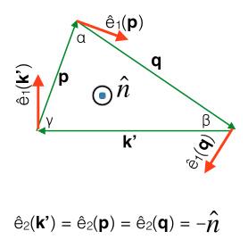
In this paper, we will derive the renormalized viscosity and energy flux by summing up contributions from all the interacting triads. Therefore, as a first step, we write down the evolution equations for in a triad. For the same, we consider a wavenumber triad with , and choose as follows [40, 28]:
| (11) |
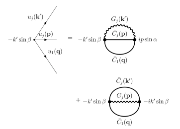
Since , we deduce that . The Craya-Herring basis vectors for the interacting wavenumbers are illustrated in Fig. 1. Note that , are the angles in front of respectively. The net nonlinear interaction is a sum over all possible triads. Hence, the equations for the components of a triad are [28]:
| (12) | |||||
| (13) | |||||
| (14) | |||||
with , and the angles , are computed for the respective triads. The equations for , , …, , denoted by , are similar:
with .
The energy flux is compactly captured by the following mode-to-mode energy transfers in the Craya-Herring basis [39, 28]:
| (18) |
with
| (20) |
for . An isotropic -dimensional divergence-free flow field has Craya-Herring components with
| (21) |
In this paper, we denote . The total kinetic energy is
| (22) | |||||
where is the one-dimensional (1D) shell spectrum, and is the surface area of the -dimensional sphere. The above equation yields the following relationship between the modal energy and 1D energy spectrum [7, 41, 27]:
| (23) |
After the above preliminary discussion on the relevant equations, we perform renormalization group (RG) and energy transfer analysis for -dimensional hydrodynamic turbulence.
III Renormalization Group Analysis of Hydrodynamic Turbulence
In this section, we derive the renormalized viscosity using the Craya-Herring basis. We follow the recursive RG method proposed by McComb, Zhou, and coworkers [13, 42, 15]. Note that the coupling constant, the coefficient in front of the nonlinear term , is unchanged under renormalization due to the Galilean invariance [8, 14]. Therefore, vertex renormalization is not required in hydrodynamic turbulence. In addition, in the recursive RG, the forcing or noise is introduced at large scales so as to produce a steady-state with Kolmogorov spectrum. Hence noise renormalization too is avoided in this scheme [13, 42, 15], and the energy spectrum is taken as . Note that such a choice for is as arbitrary as the choice of noise that yields Kolmogorov’s spectrum (as is done in noise renormalization [9]).
The evolution equations for differs from the other components. Therefore, we expect that ’s renormalized viscosity, denoted by , differs from that of others, which is denoted by . Note that the renormalized viscosities of are the same due to the symmetries of Eqs. (II-II).
III.1 Renormalization of Component
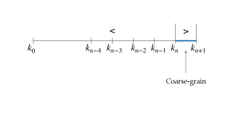
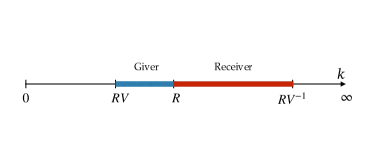
In a recursive renormalization scheme, we divide the Fourier space into wavenumber shells , where with . We perform coarse-graining or averaging over a wavenumbers band, and compute its effects on the modes with lower wavenumber. Let us assume that we are at a stage with wavenumber range of , among which the shell is coarse-grained. See Fig. 2 for an illustration.
We start with a dynamical equation for of Eq. (12). Note that . The convolution in the dynamical equation involves the following four sums:
| (24) |
because and may be either less than or greater than . As in large-eddy simulations (LES), in Eq. (24) represents the renormalized viscosity for in the wavenumber range [38, 43]. Now, we ensemble-average or coarse-grain the fluctuations at scales . After coarse-graining, the viscosity would be , which acts on the wavenumbers .
For the coarse-graining process, we assume that is time-stationary, homogeneous, isotropic, and Gaussian with zero mean, and that are unaffected by coarse-graining [5, 42, 24]. That is,
| (25) | |||||
| (26) |
Therefore, assuming weak correlation between and modes, we arrive at
| (27) | |||||
| (28) | |||||
| (29) |
Substitution of the above relations in Eq. (24) yields
| (30) |
where represents the wavenumber region . The second term of Eq. (30) enhances or renormalizes the kinematic viscosity leading to the following equation:
| (31) |
where
| (32) |
As we show below, Eq. (32) has two solutions. The first solution corresponds to the delta-correlated for which the second integral of Eq. (30) is trivially zero [44, 45, 46]. For this case,
| (33) |
That is, the viscosity is not renormalized, and it remains 0 at all scales. This corresponds to the absolute equilibrium solution of Euler equation that has [45, 44, 46]. Hence, Euler equation and the corresponding field-theoretic equations satisfy time-reversal symmetry. The second solution, which is more complex and out of equilibrium, is computed as follows.
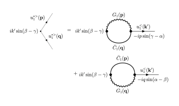
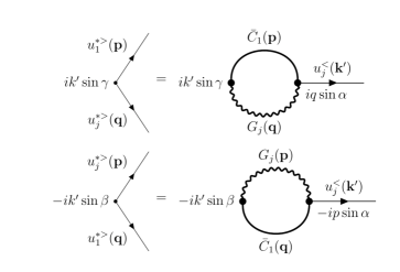
Under the quasi-gaussian approximation, the second integral of Eq. (30) vanishes to the zeroth order. Hence, we expand the second term to the first-order in perturbation that leads to the Feynman diagrams of Fig. 3. We compute the integral corresponding to the first loop diagram as follows. We expand using the Green’s function [see Eq. (13)]:
| (34) |
where . We substitute the expression of Eq. (34) in the right-hand-side of Eq. (30) and simplify the expression using the following relations [42, 24]:
| (35) | |||||
| (36) | |||||
| (37) |
In the above equations, is the unequal time correlation, whereas is the equal-time correlation. Note that of Eqs. (36, 37) is the renormalized viscosity at wavenumber . As in all field theories of turbulence, we assume that the times scales for is same as that of . Equation (35) yields , using which we deduce that the integral corresponding to the first loop diagram is
| (38) |
Now, we employ Markovian approximation [23, 41, 38]. When , the function rises sharply to unity near . Hence, the integral gets maximal contribution near . Therefore, , and
Following similar steps, we compute the integral corresponding to the second loop diagram of Fig. 3 as
Since and are proportional to , these terms can added to to yield the renormalized viscosity . In particular, using Eqs. (31, 32) we show that
where are without .
To compute , we choose in Eq. (LABEL:eq:nu1(k)). In addition, we make the following change of variables:
| (42) |
that yields a triad with and . We choose for our calculation. Zhou et al. [47] showed that yields a nearly constant value for the renormalized viscosity. McComb and Shanmugasundaram [13], and Zhou et al. [15] employed in the same range. In our RG scheme, a modified version of Zhou et al. [47], we employ (which lies within (4/3,1.8)) so that the renormalized parameter and Kolmogorov’s constant are close to the experimental values.
For the integral we employ and , where is the angle between and , as the independent variables that yields
| (43) |
where are the domain of integrations: and , in which the latter limits are obtained by setting . In this paper, we focus on spectral regime, for which is given by Eq. (23), and
| (44) | |||||
| (45) |
where is the energy flux, is the Kolmogorov constant, and is the renormalization constant for .
We substitute Eqs. (44, 45) in Eq. (LABEL:eq:nu1(k)), and simplify the expressions using trignometric identities for the triad (see Fig. 1). At , these operations yield
| (46) |
where
| (47) | |||||
| (48) |
are functions of the independent variables and . Equation (46) differs from those employed by McComb and Shanmugasundaram [13] and Zhou et al. [48] who computed the correction to [Eq. (LABEL:eq:nu1(k))] for all ’s that leads to a -dependent . In our paper, we interpret as the renormalized viscosity for wavenumbers that leads to a constant . Our scheme, which is motivated by LES [38, 43], simplifies the computation of significantly.
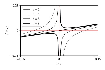
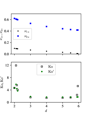
The solution is the root of [see Eq. (46)], which is illustrated in Fig. 4 for . For , we have positive and negative roots, out of which only the positive root is sensible because it leads to diminishing temporal correlation with the increase of [see Eq. (37)] and negative energy flux for in the regime. Hence, we work with positive for . In Table 1 we list for various ’s. Note that decreases gradually to zero as .
For , Eq. (46) has no root. Therefore, , the equilibrium solution of Euler equation, is the only solution for the RG equation. This is similar to Wilson’s theory [5], where the system transitions from nontrivial fixed point to guassian fixed point at . These observations indicate that is the upper critical dimension.
To determine , we compute the integral of Eq. (46) numerically. For an accurate integration, we perform the integral using Gaussian quadrature and the integral using a Romberg scheme. In addition, we employ mid-point method for computing the roots of Eq. (46). Refer to Appendix A for details on the integration schemes used in this paper. We employ Python’s scipy.integrate.romberg function whose tolerance limit is .
| 2 | 0.098 | 0.619 | 4.66 | 4.66 |
| 2.1 | 0.095 | 0.608 | 11.93 | 5.82 |
| 2.15 | 0.093 | 0.603 | 5.56 | 4.42 |
| 2.2 | 0.092 | 0.598 | 4.05 | 3.70 |
| 3 | 0.070 | 0.533 | 1.63 | 1.88 |
| 4 | 0.049 | 0.479 | 1.45 | 1.69 |
| 5 | 0.030 | 0.441 | 1.48 | 1.69 |
| 5.95 | 0.006 | 0.417 | 5.27 | 1.73 |
| 6* | 0 | 0 | - | - |
For , is the only renormalized parameter. However, higher dimensions have both and . Refer to Verma [37] for a detailed comparison of our with those reported earlier. In the next subsection, we will compute the renormalized viscosities for the , …, components.
III.2 Renormalization of () Components
For isotropic turbulence, the renormalized viscosities for the components , …, are the same. We denote this quantity as and compute it following the same steps as in Section III.1, but with Eq. (II). One of the intermediate steps in the derivation of is
| (49) |
where . In the above equation, the terms of the form contribute to viscosity renormalization. In this subsection we show that , which is expected because and with evolve differently [Eqs. (12, II)].
As in Section III.1, we employ the isotropic correlation function of Eq. (23) and
| (50) |
where is the energy flux, and is the renormalization constant for with . The second integral of Eq. (49) contributes to the viscosity renormalization, whose associated Feynman diagrams are shown in Fig. 6, and the corresponding integral is
| (51) | |||||
that contributes to the viscosity renormalization as follows:
with
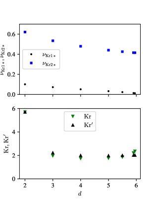
We solve for by iterating Eq. (LABEL:eq:nu2_integral) starting with a guess value of . The iterative process converges to listed in Table 1 and illustrated in Fig. 5. Since nonzero solution exists only for , Eq. (LABEL:eq:nu2_integral) implies that too is valid for . For , that corresponds to the equilibrium solution of Euler equation. Note , as illustrated in Fig. 5.
For , hydrodynamic turbulence exhibits multitudes of triads, each of which have different . Hence, for a given , the Craya-Herring vectors of Fig. 1 transform to each other (depending on the triads). Note, however, that , hence we may estimate that , which would be useful for LES. In spite of the above complications, independent evaluations of and yield valuable insights, chiefly that as , leading to the upper critical dimension of hydrodynamic turbulence as 6. The earlier works, e.g., [29], could not reach this result because they did not resolve the renormalized viscosities for the different components of the velocity field.
Using Eqs. (45, 50), we derive that for both and ,
| (54) |
In quantum field theory, we express the running coupling constant in terms of [1]. Using (for small ), we derive the beta function for using
| (55) |
or
| (56) |
Note that the beta function for the coupling constant is
| (57) |
due to Galilean invariance. These relations would be useful in relating field theory of turbulence and quantum field theory [1].
In the next section, we compute the energy flux using field theory.
IV Energy Transfers and Fluxes in dimensions
In this section, we compute the energy transfer rates and energy flux in the inertial range of hydrodynamic turbulence.
IV.1 Energy Transfers and Flux for Component
In this subsection, we will compute the mode-to-mode energy transfers among the components within a triad. We start with Eq. (II) and present the ensemble-averaged mode-to-mode energy transfer from to with the mediation of , which is
| (58) | |||||
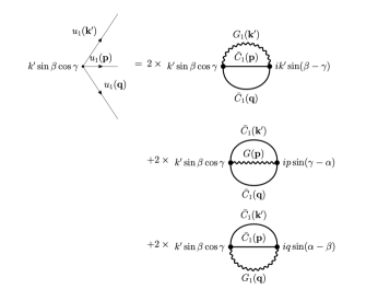
with . Following earlier literature [7, 23], we assume that the variables , , and are quasi-normal. Under this assumption, the triple correlation of Eq. (58) vanishes to the zeroth order. However, the first-order expansion of the triple correlation of Eq. (58) leads to a fourth-order correlation, that is expanded as a sum of products of two second-order correlations. The corresponding Feynman diagrams are given in Fig. 7.
Let us evaluate the integral corresponding to the first Feynman diagram of Fig. 7. Here, is expanded using the Green’s function as [see Eq. (12)]
| (60) | |||||
with . Substitution of the above in Eq. (58) leads to a fourth-order correlation, which is expanded as a sum of products of two second-order correlations:
| (61) |
Note that because and . Using the above correlations, we deduce that
Using the properties of temporal relations of Eqs. (36, 37), we deduce that
This term plus other two terms of Fig. 7 yields
| (64) |
where
| (65) | |||||
The physics in the inertial range is scale invariant, hence we employ the following transformations [7, 41]:
| (66) |
that leads to
where
| (68) |
with
| (69) | |||||
and . Note that has a dimension of , whereas is dimensionless. In Fig. 8(a,c,e) we illustrate the density plots of for respectively.
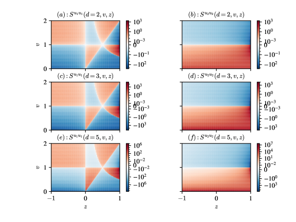
As is evident in Fig. 8(a,c,e), the function exhibits the following interesting properties:
- 1.
-
2.
takes large negative values for all ’s when . These are nonlocal reverse energy transfers from to when . These transfers are responsible for the inverse energy cascade in 2D hydrodynamic turbulence when .
- 3.
After a brief discussion on we compute the energy flux in 2D arising from the cumulative energy transfers:
| (70) |
Substitution of Eq. (LABEL:eq:Svw_u1) transforms the energy flux equation to [7, 37]
| (71) | |||||
where
| (72) |
We compute the double integral of Eq. (71) numerically. We employ Gauss-Jacobi quadrature for the integral, and Romberg iterative scheme for the integral. Refer to Section A for a brief discussion on the integration procedure.
Two-dimensional hydrodynamics has only component. Hence, is the energy flux for 2D turbulence. In the regime of 2D turbulence, we observe that indicating an inverse cascade of energy, consistent with the predictions of Kraichnan [51]. Using and , we deduce that . This is lower than that reported in experiments and numerical situations, which is approximately 6. This inconsistency is possibly due to the inability of the recursive RG schemes to capture the nonlocal interactions [37]. Note that 2D hydrodynamic turbulence involves local forward energy transfer and nonlocal inverse energy transfer, which is difficult to incorporate in RG procedure. Verma [37] employed a temporary fix for this problem by increasing the lower cutoff of the flux integral to 0.22. We find that yields , which is close to the earlier numerical and experimental results. Hopefully, in future we will understand the reason for the cutoff better.
IV.2 Energy Transfers and Fluxes for the Components with
As shown in Eq. (20), the mode-to-mode energy transfer from to [] with the mediation of is
| . | (73) |
Note that are the same for all ’s from to due to isotropy. To compute this quantity we employ the scheme described in Sec. IV.1. For simplicity, we restrict ourselves to flows for which when . Consequently, the expansion of components in terms of the Green’s function yields nonzero values, whereas the terms arising from the expansion of component vanishes identically. The Feynman diagrams associated with (for ) are illustrated in Fig. 9.
Following the same steps as in Section IV.1, the field-theoretic estimate for is
We assume that turbulence is isotropic, hence . In addition, we transform to as follows:
| (75) | |||||
with
| (76) |
In Fig. 8(b,d,f), we illustrate for . As shown in the figure, exhibits the following interesting properties:
- 1.
-
2.
for all ’s when . These transfers represent forward nonlocal energy transfers from to .
- 3.
Now we compute the energy flux that receives contributions from the components as given below:
| (77) |
hence
| (78) | |||||
where is given by Eq. (72). For Eq. (78), we perform the integral using Gauss-Jacobi quadrature, whereas the integral using Romberg iterative scheme. Note that the total energy flux in the inertial range is
| (79) |
which equals the dissipation range .
Now a brief discussion on the 3D energy flux, which is
| (80) |
Note that and appear in the denominators of Eqs. (68, 76) respectively. Since , the negative energy flux dominates positive leading to . This is a problem! Fortunately, this issue is easily resolved by employing for of Eq. (70) (as in Sec. IV.1); this procedure yields , which is in good agreement with earlier field-theoretic computations, as well as numerical and experimental results. As discussed in Sec. III.2, and are transformed to each other under the change of triads (). Therefore, we may also use that yields .
For dimension, the solution of Eq. (79) yields and for various ’s. These results are listed in Table 1 and illustrated in Fig. 5. The constant increases from to , then decreases up to , and finally increases again up to . Note that these constants are not defined for , where the equilibrium solution ( with zero flux) is valid. Thus, is the critical dimension for hydrodynamic turbulence. Also, for a given , . Hence, is inversely proportional to .
We compare our predictions with those in the past literature. Using Lagrangian renormalized approximation, Gotoh et al. [30] showed that the Kolmogorov’s constant for 3D and 4D are 1.72 and 1.31 respectively. Berera et al. [31] reported the corresponding constants to be 1.7 and 1.3 respectively. The corresponding numbers in our calculations, 1.63 and 1.45, are in general agreement with the earlier results.
Exploration of turbulence in fractal dimension remains a challenge. Lanotte et al. [52] simulated hydrodynamic turbulence in fractal dimension between 2.5 to 3. They studied variations of energy spectrum and probability distribution function of vorticity as function of fractional dimension. It will be interesting to employ similar ideas to dimension close to 2 and for much higher dimension, but we expect these numerical experiments to be very expensive. It is possible that the fractional dimension is related to the quasi-2D anisotropic turbulence that shows a transition from positive energy flux to negative energy flux with the decrease of vertical dimension [53].
V Fractional Energy Transfers
To disentangle the energy transfers between various wavenumber regimes, as well as to quantify the dependence of the energy flux on , we define fractional energy flux as follows:
| (81) | |||||
where . Based on the relations of Eq. (66), we deduce that represents the net energy transfer from the giver modes in the band to the receiver modes in the band . See Fig. 10 for an illustration.
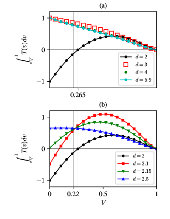
We compute for and , and plot them in Fig. 11(a, b). The plots in the figure reveal that is negative for , positive for , and 0 for . Hence, the energy flux changes sign at . The spiking in near is due to the vanishing of the energy flux (see Fig. 5). Our results are in a reasonable agreement with those of Fournier and Frisch [29] who reported the transition dimension for the energy flux to be approximately 2.06.
In 2D, changes sign from negative to positive as crosses 0.265 from left to right (see Fig. 11(a)). This feature arises due to the positive local transfers, but significant negative (inverse) nonlocal energy transfers [50, 37]. The inverse energy cascade in 2D hydrodynamics is due to the above nonlocal reverse energy transfers. For more details on local and nonlocal energy transfers, refer to Verma [37].
In the next section, we compute the renormalization and Kolmogorov’s constants for Kraichnan’s spectrum.
VI Renormalization and energy flux computations for Kraichnan’s spectrum
Kraichnan [54] argued that the sweeping effect may lead to energy spectrum for hydrodynamic turbulence. However, experiments, numerical simulations, and analytical works rule out this spectrum, and strongly support Kolmogorov’s spectrum. Still, for mathematical curiosity we explore whether spectrum satisfies the RG equation.
In the framework,
| (82) | |||||
| (83) | |||||
| (84) |
where is the large-scale fluid velocity; and are the renormalization constants for and components; and is Kraichnan’s constant (corresponding to Kolmogorov’s constant). For the energy spectrum, the Feynman diagrams and all the equations of Sections III and IV, except those for , , , , , , , , and , are unchanged. The above equations are modified to the following form (with bar):
| (85) | |||||
| (87) | |||||
| (88) | |||||
| (89) | |||||
| (90) | |||||
for . Using the revised equations we compute the new renormalization and Kraichnan’s constants for various space dimensions. We observe that has nonzero solution for , and it has no solution for . However, is a valid solution for . Hence, is the critical dimension for the Kraichnan’s spectrum as well. In Fig. 12 we present the renormalized parameters and Kraichnan’s constant for various dimensions. Note that the constants and correspond respectively to cases when and
Thus, surprisingly, Kraichnan’s spectrum and the corresponding viscosity formulas are solutions to the RG equations for . We conclude in the next section.
VII Conclusions
In this paper, we employ perturbative field theory to the incompressible Navier-Stokes equation and compute the renormalized viscosities and Kolmogorov’s constant for various space dimensions. We employ Craya-Herring basis that simplifies the calculations considerably. We summarize our findings as follows.
-
1.
For space dimension less than 6, Kolmogorov’s spectrum is a solution of the RG equation with the renormalized viscosity scaling as , where are the prefactors for the components of the Craya-Herring basis. These constants are computed using the recurrence relation for the renormalized viscosity. Our computed constants are in general agreement with earlier results. These solutions are out of equlibrium when the energy flux is nonzero.
-
2.
The renormalization constants are functions of space dimension. Interestingly gradually decreases to zero at . Our detailed calculations show that the solutions for are out of equilibrium, but they merge with equilibrium solution at . Thus, is the critical upper dimension.
-
3.
For , the viscosity remains unnormalized (), and the equilibrium solution of Euler equation, , satisfies the RG equation. Note that the energy flux vanishes under this condition. Adzhemyan et al. [32] showed that the Kolmogorov constant which leads the vanishing energy flux, , as . In similar lines, Fournier et al. [33] showed that intermittency vanishes as . These observations too indicate Gaussianity of the velocity field at large , consistent with our results. Our renormalization calculation indicates that the upper critical dimension for hydrodynamic turbulence is 6. Thus, we can argue that the nonequilibrium solution with nonzero energy flux transitions to the equilibrium solution with . Note that the equilibrium solution with respects time-reversal symmetry. However, the nonequilibrium solution with finite and nonzero energy flux breaks the time-reversal symmetry [55].
-
4.
Using field theory, we compute the mode-to-mode energy transfers, energy fluxes, and Kolmogorov’s constant for . The energy flux is negative for , whereas it is positive for . The transition dimension is in reasonable agreement with the predictions of Fournier and Frisch [29], according to which the energy flux changes sign near .
-
5.
Our results, in particular Kolmogorov’s constant, are in agreement with previous works for 4D turbulence simuations [30, 31]. Note that simulation of turbulent flows for is very expensive due to large grid size. Simulation of turbulence in fractional dimension is of interest [52], but these simulations too require considerable computing resources.
-
6.
The present work does not include intermittency correction, which is more complex to compute. Researchers have employed multi-loop field-theoretic calculations (e.g., [56]) and Lagrangian field-theory calculations (e.g., [57]) to quantify intermittency in turbulence. It will be interesting to use Craya-Herring basis for intermittency computations.
-
7.
Interestingly, Kraichnan’s energy spectrum, which is inspired by the sweeping effect, too satisfies the recursive RG equation for hydrodynamic turbulence. Note however that energy spectrum is ruled out based on numerical and experimental findings, as well as from analytical works such as Kolmogorov’s K41 theory [58].
In summary, field-theoretic tools provide valuable insights into hydrodynamic turbulence.
Acknowledgements: The author thanks Soumyadeep Chatterjee for help in generating the Feynman diagrams. He also thanks Srinivas Raghu, Rodion Stepanov, Jayant Bhattacharjee, Krzysztof Mizerski, and anonymous referees for comments on the paper. I got valuable suggestions on the paper during the discussion meeting “Field Theory and Turbulence” hosted by International Centre for Theoretical Studies, Bengaluru. This work is supported by Science and Engineering Research Board, India (Grant numbers: SERB/PHY/20215225 and SERB/PHY/2021473).
Appendix A Evaluation of the Renormalization and Energy Flux Integrals
For the RG procedure, the integrals of Eqs. (46, LABEL:eq:nu2_integral) are finite because they are performed in the band and . Here, we employ the Gaussian quadrature for the integral and a Romberg scheme for the integral. This procedure yields finite and accurate results. However, the integrals for the energy flux are singular [1] and they need special attention.
The energy-flux integral is of the following form:
| (91) |
where involves singularities. For accurate evaluation of integration, we employ the Gauss-Jacobi quadrature:
| (92) |
where is the th root of Jacobi polynomials, and is the corresponding weight. Note that is evaluated at . The Gauss-Jacobi quadrature yields finite answer for these singular integrals. We employ a Romberg iterative scheme for the subsequent integration.
References
- Peskin and Schroeder [1995] M. E. Peskin and D. V. Schroeder, An Introduction To Quantum Field Theory (The Perseus Books Group, Reading, MA, 1995).
- Lancaster and Blundell [2014] T. Lancaster and S. J. Blundell, Quantum field theory for the gifted amateur (Oxford University Press, Oxford, 2014).
- Zinn-Justin [1993] J. Zinn-Justin, Quantum field theory and critical phenomena, 2nd ed., Oxford science publications (Clarendon Press, Oxford, 1993).
- Vasil’ev [2004] A. N. Vasil’ev, The Field Theoretic Renormalization Group in Critical Behavior Theory and Stochastic Dynamics (CRC Press, Boca Raton, FL, 2004).
- Wilson and Kogut [1974] K. G. Wilson and J. Kogut, Phys. Rep. 12, 75 (1974).
- Ma [1985] S.-K. Ma, Statistical Mechanics (World Scientific, Singapore, 1985).
- Kraichnan [1959] R. H. Kraichnan, J. Fluid Mech. 5, 497 (1959).
- Forster et al. [1977] D. Forster, D. R. Nelson, and M. J. Stephen, Phys. Rev. A 16, 732 (1977).
- Yakhot and Orszag [1986] V. Yakhot and S. A. Orszag, J. Sci. Comput. 1, 3 (1986).
- Adzhemyan et al. [1999] L. T. Adzhemyan, N. V. Antonov, and A. N. Vasiliev, Field Theoretic Renormalization Group in Fully Developed Turbulence (CRC Press, Boca Raton, FL, 1999).
- DeDominicis and Martin [1979] C. DeDominicis and P. C. Martin, Phys. Rev. A 19, 419 (1979).
- Martin et al. [1973] P. C. Martin, E. D. Siggia, and H. A. Rose, Phys. Rev. A 8, 423 (1973).
- McComb and Shanmugasundaram [1983] W. D. McComb and V. Shanmugasundaram, Phys. Rev. A 28, 2588 (1983).
- McComb [2014] W. D. McComb, Homogeneous, Isotropic Turbulence: Phenomenology, Renormalization and Statistical Closures (Oxford University Press, 2014).
- Zhou et al. [1988] Y. Zhou, G. Vahala, and M. Hossain, Phys. Rev. A 37, 2590 (1988).
- Canet [2022] L. Canet, J. Fluid Mech. 950, P1 (2022).
- Eyink [1993] G. L. Eyink, Phys. Rev. E 48, 1823 (1993).
- Moriconi [2004] L. Moriconi, Phys. Rev. E 70, 025302 (2004).
- Arad et al. [1999] I. Arad, V. L’vov, and I. Procaccia, Phys. Rev. E 59, 6753 (1999).
- Biferale and Procaccia [2005] L. Biferale and I. Procaccia, Phys. Rep. 414, 43 (2005).
- Bos and Rubinstein [2013] W. J. Bos and R. Rubinstein, J. Fluid Mech. 733, 158 (2013).
- Kaneda [2007] Y. Kaneda, Fluid Dyn. Res. 39, 526 (2007).
- Orszag [1973] S. A. Orszag, in Les Houches Summer School of Theoretical Physics, edited by R. Balian and J. L. Peube (1973) p. 235.
- Zhou [2010] Y. Zhou, Phys. Rep. 488, 1 (2010).
- Olla [1991] P. Olla, Phys. Rev. Lett. 67, 2465 (1991).
- Nandy and Bhattacharjee [1995] M. K. Nandy and J. K. Bhattacharjee, Int. J. Mod. Phys. B 09, 1081 (1995).
- Verma [2004] M. K. Verma, Phys. Rep. 401, 229 (2004).
- Verma [2019a] M. K. Verma, Energy transfers in Fluid Flows: Multiscale and Spectral Perspectives (Cambridge University Press, Cambridge, 2019).
- Fournier and Frisch [1978] J. D. Fournier and U. Frisch, Phys. Rev. A 17, 747 (1978).
- Gotoh et al. [2007] T. Gotoh, Y. Watanabe, Y. Shiga, T. Nakano, and E. Suzuki, Phys. Rev. E 75, 016310 (2007).
- Berera et al. [2020] A. Berera, R. D. J. G. Ho, and D. Clark, Phys. Fluids 32, 085107 (2020).
- Adzhemyan et al. [2008] L. T. Adzhemyan, N. V. Antonov, P. B. Gol’din, T. L. Kim, and M. V. Kompaniets, J. Phys. A: Math. Theor. 41, 495002 (2008), 0809.1289 .
- Fournier et al. [1978] J. D. Fournier, J. D. Fournier, U. Frisch, and H. A. Rose, J. Phys. A: Math. Theor. 11, 187 (1978).
- Craya [1958] A. Craya, Contribution à l’analyse de la turbulence associée à des vitesses moyennes, Ph.D. thesis, Université de Granoble (1958).
- Herring [1974] J. R. Herring, Phys. Fluids 17, 859 (1974).
- Sagaut and Cambon [2018] P. Sagaut and C. Cambon, Homogeneous turbulence dynamics, 2nd ed. (Cambridge University Press, Cambridge, 2018).
- Verma [2023] M. K. Verma, arXiv , arXiv:2309.05207 (2023).
- Lesieur [2008] M. Lesieur, Turbulence in Fluids (Springer-Verlag, Dordrecht, 2008).
- Dar et al. [2001] G. Dar, M. K. Verma, and V. Eswaran, Physica D 157, 207 (2001).
- Waleffe [1992] F. Waleffe, Phys. Fluids A 4, 350 (1992).
- Leslie [1973] D. C. Leslie, Developments in the theory of turbulence (Clarendon Press, Oxford, 1973).
- McComb [1990] W. D. McComb, The physics of fluid turbulence (Clarendon Press, Oxford, 1990).
- Nagarajan et al. [2003] S. Nagarajan, S. K. Lele, and J. H. Ferziger, Journal of Computational Physics 191, 392 (2003).
- Onsager [1949] L. Onsager, Il Nuovo Cimento 6, 279 (1949).
- Lee [1952] T. D. Lee, Quart. Appl. Math. 10, 69 (1952).
- Kraichnan [1973] R. H. Kraichnan, J. Fluid Mech. 59, 745 (1973).
- Zhou et al. [1997] Y. Zhou, G. Vahala, and W. D. McComb, Renormalization Group (RG) in Turbulence: Historical and Comparative Perspective, Tech. Rep. ICAS-97-36 (1997).
- Zhou et al. [1989] Y. Zhou, G. Vahala, and M. Hossain, Phys. Rev. A 40, 5865 (1989).
- Domaradzki and Rogallo [1990] J. A. Domaradzki and R. S. Rogallo, Phys. Fluids A 2, 414 (1990).
- Verma et al. [2005] M. K. Verma, A. Ayyer, O. Debliquy, S. Kumar, and A. V. Chandra, Pramana-J. Phys. 65, 297 (2005).
- Kraichnan [1971] R. H. Kraichnan, J. Fluid Mech. 47, 525 (1971).
- Lanotte et al. [2015] A. S. Lanotte, R. Benzi, S. K. Malapaka, F. Toschi, and L. Biferale, Phys. Rev. Lett. 115, 264502 (2015), 1505.07984 .
- Alexakis and Biferale [2018] A. Alexakis and L. Biferale, Phys. Rep. 767-769, 1 (2018).
- Kraichnan [1964] R. H. Kraichnan, Phys. Fluids 7, 1723 (1964).
- Verma [2019b] M. K. Verma, Eur. Phys. J. B 92, 190 (2019b).
- Adzhemyan et al. [2003] L. T. Adzhemyan, N. Antonov, M. Kompaniets, and A. Vasil’ev, Int. J. Mod. Phys. B 17, 2137 (2003).
- Falkovich et al. [2001] G. Falkovich, K. Gawȩdzki, and M. Vergassola, Rev. Mod. Phys. 73, 913 (2001).
- Kolmogorov [1941] A. N. Kolmogorov, Dokl Acad Nauk SSSR 30, 301 (1941).