Vortices in the Many-Body Excited States of Interacting Bosons in Two Dimension

Abstract

Quantum vortices play an important role in the physics of two-dimensional quantum many-body systems, though they usually are understood in the single-particle framework like the mean-field approach. Inspired by the study on the relations between solitons and yrast states, we investigate here the emergence of vortices from the eigenstates of a $N$-body Hamiltonian of interacting particles trapped in a disk. We analyse states that appear by consecutively measuring the positions of particles. These states have densities, phases, and energies closely resembling mean-field vortices. We discuss similarities, but also point out purely many-body features, such as vortex smearing due to the quantum fluctuation of their center. The ab initio analysis of the many-body system, and mean-field approaches are supported by the analysis within the Bogoliubov approach.

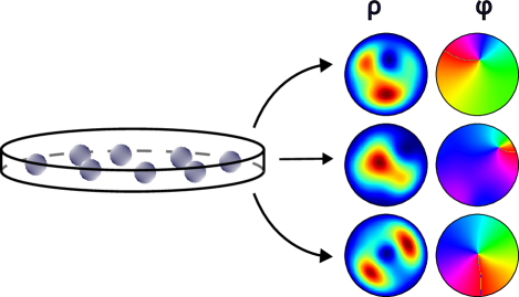
Figure 1: Graphical abstract: We study the many-body wave function of interacting bosons on a disk to detect vortices that become apparent after position measurement.

I Introduction

Mean-field (MF) approaches are often the only way to tackle quantum many-body systems and characterise their non-linear effects. At the same time, the interpretation of the MF results in terms of the underlying exact model is sometimes difficult and counter-intuitive. For instance, non-linear effects such as solitons or vortices appear naturally in mean-field frameworks as solutions of dynamical, time-dependent, single-particle, and non-linear mean-field equations. On the other hand, the ab initio model is the linear, many-body Schrödinger equation. Furthermore, it has been shown that the gray solitons, constantly moving non-linear waves known from the MF approach, are related to the non-moving many-body states, which are actually eigenstates of the many-body Hamiltonian [1, 2].

The relation between mean-field solitons and the eigenstates of the many-body Lieb-Liniger model [3, 4], so-called yrast states [5] was a subject of many papers [6, 7, 8, 9, 10, 11, 12, 13, 14]. In between, it has been found that dark soliton, robust dip in a gas density, emerge via breaking symmetry of the system initiated in the yrast state. The symmetry may be broken by simply “measuring” part of the system [7, 8], which in cold gases will happen spontaneously due to particle losses [9]. On the other hand, if the gas is prepared in a product state, with all atoms occupying the mean-field soliton, one finds within Bogoliubov theory quantum correction to this state – the black MF soliton has quantum fluctuations of its position [15] due to anomalous negative mode. The effect of these fluctuations is to gray out the soliton, even though it appears black in the MF description.

The aim of this paper is to put the research further into a study of emergence of 2D vortices out of the many-body yrast states. Quantum vortices, understood via MF approach, play an important role in many contexts, demonstrated in a number of experiments, on rotated superfluid [16], on vortex lattice [17, 18, 19], quantum turbulent gas [20] or the Berezinsky-Kosterlitz transition [21] (see [22] for more information on vortices in ultracold quantum gases). Ongoing research on vortices in 3D turbulence is making use of AI techniques for analyzing numerical and experimental results, assuming mean-field description. While mean-field methods are commonly employed in these studies, it is essential to acknowledge their limitations. The observation of unexpected quantum droplets [23], which arise due to the quantum corrections [24], highlights the need to further study model systems at the quantum many-body level and compare them with the MF approach.

In the present work, we focus on a gas of atoms with short-range interactions inside a 2D circular plaquette. Unlike in 1D, there are no analytical solutions for vortices – neither in the many-body nor in the MF approach. In fact, even numerically, it is not straightforward to find such dynamical solutions to the MF, that would posses a single vortex with core outside the center of the trap. Our starting points are the many-body yrast states – states minimizing energy at fixed momentum, which we find using the exact diagonalization method. We show that during consecutive “measurements” of positions of particles initiated in an yrast state, one reveals vortices. They may appear off the plaquette center, and at random positions, but are robust dynamically, as confirmed by evolving it with the mean-field equations. In a sense, our complicated procedure serves approximate solution to the MF approach. Special attention is paid to the states with the angular momentum proportional to the number of atoms. In these cases, one expects vortices appearing in the center of the disk. We show that even in this simplest case, the position of the vortex revealed from the quantum states fluctuates. As a result, the average density profile differs between the MF and many-body approach, even in this case. The differences are attributed to the quantum fluctuations, as confirmed by the Bogolubov analysis, similarly to the case of "graying" of the 1D black soliton [15].

In Sec. II we present our model. Sec. III is devoted to the ground state, for which MF gives very good results, for as few as $6$ atoms. In Sec. IV we show that vortices are not apparent in the densities, but they emerge in a stochastic process mimicking measurements on many-body excited states. We conclude in Sec V.

II Model

We illustrate our findings for 2D vortices on an example of system of bosons interacting via contact potential and trapped inside a quasi-2 dimensional disk, i.e. assuming infinite potential outside a disk of radius $R$ and neglecting the $Z$ direction. Our Hamiltonian of interest in the second quantized form reads

$$\hat{H}=\int\hat{\psi}^{\dagger}\left(-\frac{\hbar^{2}}{2M}\nabla^{2}\right)\hat{\psi}\mathop{}\!\mathrm{d}{\bm{r}}+\frac{g}{2}\int\hat{\psi}^{\dagger}\hat{\psi}^{\dagger}\hat{\psi}\hat{\psi}\mathop{}\!\mathrm{d}{\bm{r}},$$ (1)

where $M$ is the atomic mass, $g$ is the interaction coupling constant, $\bm{r}=[x,\,y]$ is a two-dimensional position and $\hat{\psi}(\bm{r})$ is the field operator obeying the bosonic commutation relations $[\hat{\psi}(\bm{r}),\,\hat{\psi}^{\dagger}(\bm{r}^{\prime})]=\delta(\bm{r}-\bm{r}^{\prime})$. The Hamiltonian assumes silently, that the interactions are described by the Dirac delta potential $g\,\delta(\bm{r}-\bm{r}^{\prime})$. Noteworthy, this simplistic model of interactions in 2D is well-defined for MF, but may lead to mathematical and numerical problems in a many-body approach. Therefore we discuss below the details of our numerical implementation and show the test of numerical convergence in Appendix B.

Firstly, we decompose the quantum field operator in a single-particle basis as follows:

$$\hat{\psi}(r,\phi)=\sum_{j}\psi_{j}(r,\phi)\,\hat{a}_{j},$$ (2)

where index $j$ runs over all single-particle states. For our trap geometry those are given as products of Bessel functions of the first kind and phase factors

$$\psi_{j}(r,\phi)=A_{j}J_{m_{j}}\left(\alpha_{j}r/R\right)e^{im_{j}\phi}.$$ (3)

For convenience, we label the single-particle eigenstates with a multi-index $j$ that encodes both the magnetic quantum number $m$ and the quantum number labeling the radial eigenstates. The integer $m_{j}$ represents the angular momentum of a given state in units of $\hbar$. For a given $m_{j}$, all radial excitations are described by the first-kind $m_{j}$-th Bessel functions, but rescaled by the factor $\alpha_{j}$. The scaling factors $\alpha_{j}$, which distinguish different radial excitations for a given $m$, are consecutive zeros of the $m_{j}$-th Bessel function. This construction guarantees that the boundary condition $\psi_{j}(R,\phi)=0$ is always satisfied. Finally, $A_{j}$ is the normalization constant. Examples of the radial part of the wavefunctions are given in Fig. 2. Energy of such a single particle state follows the formula

$$E_{j}=\frac{\hbar^{2}\alpha_{j}^{2}}{2MR^{2}}.$$ (4)

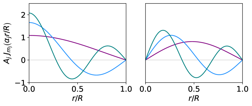
Figure 2: Examples of radial parts of the single particle states used in numerics, Eq. (3) for $m_{j}=0$ (left) and $m_{j}=1$ (right). All radial parts for $m_{j}=0$ are the $0$th Bessel functions, but rescaled by $\alpha_{j}$ (with $\alpha_{j}$ being zeros of the $0$th bessel function). Similarly, all radial parts for $m_{j}=1$ equal to rescaled the 1st Bessel function.

Inserting (2) into (1) we obtain the Hamiltonian in terms of the creation and annihilation operators

$$\hat{H}=\sum_{j}E_{j}\hat{a}_{j}^{\dagger}\hat{a}_{j}+g\pi\sum_{ijkl}V_{ijkl}\delta^{m_{i}+m_{j}}_{m_{k}+m_{l}}\hat{a}_{i}^{\dagger}\hat{a}_{j}^{\dagger}\hat{a}_{k}\hat{a}_{l},$$ (5)

where $V_{ijkl}$ is fourfold Bessel function integral

$$V_{ijkl}=A_{i}A_{j}A_{k}A_{l}\int_{0}^{R}rJ_{m_{i}}J_{m_{j}}J_{m_{k}}J_{m_{l}}\mathop{}\!\mathrm{d}{r}.$$ (6)

Note that the Hamiltonian is invariant under rotation, which implies that angular momentum is conserved. As a result, the Kronecker delta appears in Eq. (5). This invariance also implies that all eigenstates of the Hamiltonian can be chosen to be also eigenstates of the angular momentum operator $\hat{L}_{z}$.

Our objects of interest are the excited states of the above Hamiltonian (5), that minimize the energy at a fixed angular momentum, so called yrast states [5]. In our paper we will compare them with the states arising in the simplistic description of the system, the Gross-Pitaevskii equation (GPE), and the Bogoliubov approximations.

Mean-field approximation In the MF approach, it is usually assumed that every particle resides in the same state $\psi_{\mathrm{GP}}(\bm{r},t)$ and its dynamics are governed by the GPE

$$i\hbar\frac{\partial}{\partial t}\psi_{\mathrm{GP}}=\left(-\frac{\hbar^{2}}{2M}\nabla^{2}+g(N-1)|\psi_{\mathrm{GP}}|^{2}\right)\psi_{\mathrm{GP}},$$ (7)

with stationary solutions obeying the time-independent GPE

$$\left(-\frac{\hbar^{2}}{2M}\nabla^{2}+g(N-1)\left|\psi_{\mathrm{GP}}\right|^{2}\right)\psi_{\mathrm{GP}}=\mu\,\psi_{\mathrm{GP}}.$$ (8)

Imposing the constrain $\psi_{\mathrm{GP}}(\bm{r})=f(r)e^{i\phi}$ yields a solution with single vortex at the center. In contrast, the ground state can be found assumming $\psi_{\mathrm{GP}}(\bm{r})=f(r)$, which depends only on the distance from the center.

The GPE is the simplest version of the mean-field theory for our system – via non-linear term a single particle “feel” all other particles due to effective potential $g(N-1)\left|\psi_{\rm GP}\right|^{2}$ created by all other particles. We will not invoke in this paper more elaborated mean-field versions, like the ones based on the density-functional theories.

Instead we will invoke the Bogoliubov approximation – many-body approach, but based on the assumption that almost all atoms occupy the MF orbital $\psi_{\rm GP}$, with only a small fraction of atoms in other single-particle states [25, 26]. Technically, one has to find the Bogoliubov modes $u(\bm{r})$ and $v(\bm{r})$ that obey the Bogoliubov-de Gennese equations:

$$\begin{pmatrix}\hat{H}_{\mathrm{GP}}+gN|\psi_{\mathrm{GP}}|^{2}&gN\psi_{\mathrm{GP}}^{2}\\ -gN\psi_{\mathrm{GP}}^{*2}&-\hat{H}_{\mathrm{GP}}-gN|\psi_{\mathrm{GP}}|^{2}\end{pmatrix}\begin{pmatrix}u_{n}\\ v_{n}\end{pmatrix}=\epsilon_{n}\begin{pmatrix}u_{n}\\ v_{n}\end{pmatrix},$$ (9)

where

$$\hat{H}_{\mathrm{GP}}=-\frac{\hbar^{2}}{2M}\nabla^{2}+gN|\psi_{\mathrm{GP}}|^{2}-\mu.$$ (10)

Solutions can be classified into three families: the “$+$ family”, the “$-$ family”, and the “0 family”. These names correspond to the normalization of the expression $\langle u_{n}|u_{n}\rangle-\langle v_{n}|v_{n}\rangle$, which equals $+1$, $-1$ and $0$, respectively [25]. Having $u_{n}(\bm{r})$ and $v_{n}(\bm{r})$ one is in position to compute quantities to characterize the system, as the ones listed below.

Quantities In our comparisons between the many-body and GPE approaches, we compute energies and density profiles and then track the differences with the help of the correlation functions.

The energy of the many-body yrast states comes simply from exact diagonalization of the hamiltonian (5). It is compared, wherever possible, with the mean-field energy:

$$E_{\rm GP}=N\int\psi^{*}_{\rm GP}\left(-\frac{\hbar^{2}}{2M}\nabla^{2}+\frac{g(N-1)}{2}\left|\psi_{\rm GP}\right|^{2}\right)\psi_{\rm GP}\mathop{}\!\mathrm{d}{\bm{r}},$$ (11)

and the ground state energy approximated as in the Castin-Dum approach [27]:

$$E_{\mathrm{BdG}}=E_{\mathrm{GP}}-\sum_{n\in\mathrm{``+family^{\prime\prime}}}\epsilon_{n}\langle v_{k}|v_{k}\rangle.$$ (12)

Another figure of merit is the gas density. In MF the density is simply $N|\psi_{GP}|^{2}$. For many-body system, one has to compute the single particle density matrix (SPDM)

$$\rho(\bm{r},\bm{r}^{\prime}):=\langle\Psi|\hat{\psi}^{\dagger}(\bm{r}^{\prime})\hat{\psi}(\bm{r})|\Psi\rangle.$$ (13)

Its diagonal, $\rho(\bm{r})=\rho(\bm{r},\bm{r})$, yields information about the average density of particles in the many-body state $|\Psi\rangle$.

The SPDM can be used to test the assumptions underlying MF and BdG approaches, that have the validity range restricted to the weakly interacting limits. Diagonalization of SPDM yields the expansion

$$\rho(\bm{r},\bm{r}^{\prime})=N\sum_{i}\lambda_{i}\psi_{i}^{*}(\bm{r}^{\prime})\psi_{i}(\bm{r}),$$ (14)

where sum of the coefficients $\lambda_{i}$ is equal to $1$. Regime of weak interactions corresponds to situations where majority of the system lies in a single state, say $\psi_{0}$, with its eigenvalue $\lambda_{0}$ being close to $1$, that is $\lambda_{0}\gg\lambda_{i}$ for $i\neq 0$.

The value of $\lambda_{0}$ can be compared to the MF fraction $(N-\langle\delta\hat{N}\rangle)/N$ of particles in condensate, where $\langle\delta\hat{N}\rangle$ is the average number of particles out of condensate and can be calculated from BdG solution using formula [25, 26]

$$\langle\delta\hat{N}\rangle\simeq\sum_{n\in\mathrm{``+family^{\prime\prime}}}\langle v_{n}|v_{n}\rangle.$$ (15)

III Ground state

Figure 3: Energy per atom for states with $N=10$ particles as a function of coupling constant $g$ obtained from the exact diagonalization (solid lines), GPE approach (black dashed lines) and Bogoliubov approach (red dot-dashed lines). The lower curves correspond to the ground state, i.e. $0$ total angular momentum, whereas the upper ones to the states minimizing energy with total angular momentum equal to the total number of particles.

To ensure that MF and MB (many-body) approaches are mutually consistent, we begin by investigating the ground state. In Fig. 3 we show energy of ground state obtained from exact diagonalization (blue line) calculated for different coupling constants $g$. In the regime of weak interactions, this line overlaps with results from the mean-field GPE calculations (black line) up to interactions around $gN\approx 5$. The MF energy as proportional to $g$, is just a straight line that gives a correct slope to the exact energy at $g=0$ but it does not capture bending off the energy curve. The latter behaviour is well reproduced by the energy computed within the BdG approach (dot-dashed line).

To illustrate further the consistency between different approaches we check whether indeed until $gN\approx 5$, the assumption underlying MF and BdG is fulfilled, i.e. if the system is dominated by a single mode. Data for such analysis is illustrated in Fig. 4 showing the relative occupation of the dominant orbital, i.e. $\lambda_{0}$ from equation (14). As expected, up to $gN\approx 5$, practically all atoms reside in a single orbital in the ground state.

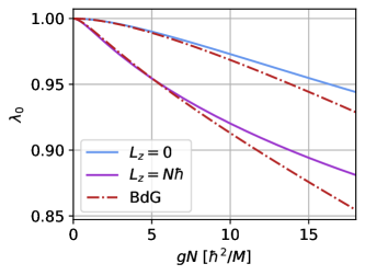
Figure 4: Condensed fraction of a system described by coefficient $\lambda_{0}$ from equation (14) as a function of the interaction strength. Calculations were performed for $N=10$ particles in the ground state (blue line) and the yrast state with angular momentum $N\hbar$ (purple line). The red dot-dashed lines illustrate the results obtained from the Bogoliubov approach.

To complete the analysis of the ground state we also compare density profiles, see Fig. 5. It shows the cross-section of MF solution $N|\psi_{\mathrm{GP}}|^{2}$ and the diagonal of SPDM, $\rho(\bm{r})$, for some selected values of the interaction strength $gN$. The density profiles are very similar, even for substantially large interaction strengths.

Figure 5: Ground state density of particles obtained from MF calculations (black dashed) and SPDM from exact diagonalization (blue solid). Calculations were performed for $N=6$ particles, the interaction strength $gN$ is given in units $\hbar^{2}/M$. Up to the largest considered value $gN=18$, both curves can be seen to overlap.

To conclude this part – in the weakly interacting regime, i.e. as long as the depletion of the condensate remains small ($\lambda_{0}\approx 1$), the energy and the density profiles are well predicted by the MF approach. In this case, comparing densities is straightforward: the single-particle density obtained from the density matrices of the many-body ground states agrees with the MF densities $N|\psi_{\rm GP}|^{2}$. This indicates a lack of substantial quantum correlations between atoms. In the following, we discuss the yrast states for which the situation is much more subtle.

IV Yrast states

We now turn to the analysis of the eigenstates minimizing energy at a fixed angular momentum, so called yrast states. We will denote the quanta of angular momenta with integer $l$, which will correspond to the value of the angular momentum equal to $l\hbar$. The case of $l=0$ corresponds to the ground state of the system described in the preceding section. We expect that yrast states with $l\neq 0$ contain quantum vortices.

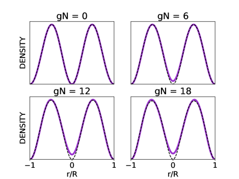
Figure 6: Yrast state density of particles obtained from MF calculations (black dashed) and SPDM from exact diagonalization (purple solid). Calculations were performed for $N=6$ particles and angular momentum $L_{z}=N\hbar$, the interaction strength $gN$ is given in units $\hbar^{2}/M$.

We begin our discussion with the special case $l=N$, where the angular momentum is evenly distributed among all the particles, each carrying $\hbar$. Then, each atom shall rotate with angular momentum $\hbar$ around the disc center, and all atoms altogether will form a single vortex. Similarly to the $l=0$ case, we compare energies (Fig. 3), the quantum depletion (Fig. 4), and the densities (Fig. 6) calculated using the ab initio and MF approaches. Unlike in the ground state case, as the interaction strength increases, differences in results of these two approaches become apparent. The quantum depletion grows much quicker with interaction, as compared with the ground state case. This implies discrepancies in the gas densities. Although the density cross-sections look very similar in both approaches, the MF densities deviates from the SPDM in the center of the system – the density at the center always vanishes in the MF approximation, whereas it is more and more filled with matter in the fully quantum analysis, at least if it comes to the diagonal of a single particle density matrix. We will postpone for a while discussion of our interpretation of the quantum case. The Reader may know similar effect, from the physics of vortices in fermionic superfluid [28] or from the discussion of graying bosonic solitons due to anomalous Bogoliubov mode [15, 29].

More puzzling is the case $0<l<N$. In this case, different scenarios are possible to imagine – off-centered vortex or vortices, possibly rotating around the center. Such solutions clearly wouldn’t be found as a stationary solution in MF (even in a rotating frame) – one should invoke the time-dependent GPE. We did not solve directly GPE to look for such states. Instead, we study this case starting from the many-body approach, and finding yrast state using exact diagonalization method. We show the SPDM for $l=N/2$ in Fig. 7. This SPDM does not give a clear view of the system. In particular it shows no vortices. The analysis for the yrast states at a fixed angular momentum $0<l\hbar<N\hbar$ looks as follows: (i) one cannot find easily these states using MF (ii) the density obtained from the single-particle reduced density matrix, Eq. (13), change substantially with interaction and does not show any vortex/vortices. Therefore we use a more subtle approach to study high-order correlation function, as described below.

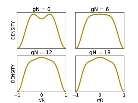
Figure 7: The single-particle density (SPDM) $\rho(\bm{r})$ as a function of a position of a system in an yrast states with angular momentum $L_{z}=N\hbar/2$, obtained via exact diagonalization. There is no clear indication of where the vortex might be located. Parameters: $N=6$ particles, angular momentum $L_{z}=3\hbar$. The interaction strength $gN$ is expressed in units of $\hbar^{2}/M$.

To this end, we use a procedure similar to the one introduced to explain an interference pattern arising in the system in a Fock state [30], also used to find solitons within 1D yrast states [29, 7]. The procedure relies on drawing (“measuring”) positions one-by-one from MB state $|\Psi\rangle$ (see Appendix A for details). One ends up with $N-1$ points $\bar{\bm{r}}_{1},\dots,\bar{\bm{r}}_{N-1}$, which then enter as parameters to the conditional wave function

$$\psi_{\textrm{cond}}(\bm{r})\propto\langle\bar{\bm{r}}_{1},\ldots,\bar{\bm{r}}_{N-1},\bm{r}|\Psi\rangle,$$ (16)

that is dependent only on one position $\bm{r}$, but it is stochastic. Note that $|\psi_{\textrm{cond}}(\bm{r})|^{2}$ is proportional to the $N$-th order correlation function

$$G_{N}=\langle\hat{\psi}^{\dagger}(\bm{r}_{1})\ldots\hat{\psi}^{\dagger}(\bar{\bm{r}}_{N-1})\hat{\psi}^{\dagger}(\bm{r})\hat{\psi}(\bm{r})\hat{\psi}(\bar{\bm{r}}_{N-1})\ldots\hat{\psi}(\bar{\bm{r}}_{1})\rangle.$$ (17)

We search for vortices within the conditional wavefunctions $\psi_{\mathrm{cond}}$, or in other words – within the high-order correlation function.

Few conditional wave functions for $N=6$ particles, $gN=6\hbar^{2}/M$ and $l=N/2$ are presented in Fig. 8 (a). In most cases one observes a single vortex although its position differs between realisations. To verify whether the vortex-like states emerging in the measuring procedure are related to the MF vortices, we use $\psi_{\rm cond}(\bm{r})$ as initial states for GPE equation and see their dynamics – as in the movie in the Supplemental Material . We found that the vortices are dynamically stable - they only rotate around the disc center without substantial distortion. One other hand, the density averaged over many measurements, that correspond to the SPDM, will show no vortices – they will be hidden due to the large dispersion in the random position of the vortex core. In the case $l=N$ (Fig. 8 (b)) the dispersion in the vortex position is much smaller, consistent with a clear vortex in the disc center shown in the SPDM in Fig. 6, just slightly greyed-out.

The dispersion around the center of the disk for $l=N$ can also be analyzed using the BdG approach. Numerically, we find the vortex with $l=N$ using the GPE equation and then study its excitations using the BdG equation. Our analysis reveals two modes that contribute most significantly to the quantum depletion. They have, approximately equal contributions. One of them is a negative energy anomalous mode. The densities $|v|^{2}$ of these modes are shown in Fig. 9, along with the vortex profile. The positive energy mode is located within the center of the vortex and is responsible for filling the vortex core visible in the SPDM in Fig. 6. The presence of this mode is also compatible with the random vortex position in the conditional wavefunction $\psi_{\rm cond}$; the distribution of these positions is likely related to the width of this mode. On the other hand, the anomalous mode is located near the peaks of the MF solution’s cross-section, effectively flattening it near the maximum.

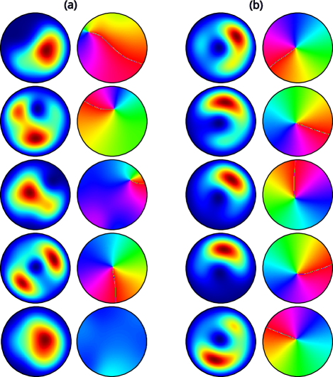
Figure 8: Density and phase of exemplary conditional wave functions (16) for $N=6$ particles, interaction strength $gN=6\hbar^{2}/M$ and the total angular momentum $N\hbar/2=3\hbar$ (a) and $N\hbar=6\hbar$ (b). In both panels there are two columns – the left one for the density and the right one for the phase of $\psi_{\rm cond}$ In both cases, a vortex, if appears, emerges off-centered, while in (a) the variation of its position is much greater.

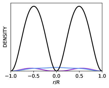
Figure 9: The cross section of the MF density $|\psi_{\mathrm{GP}}|^{2}$ (black solid) is compared with the densities $|v_{k}|^{2}$ of two BdG modes that contribute the most to depletion, one with positive energy (blue solid) and one with negative energy (purple solid). For normalization, the GPE solution is scaled by $(N-\langle\delta N\rangle)/N$, while the BdG mode by $\langle\delta N\rangle/N$. Computations were performed for $N=10$ and $gN=12\ \hbar^{2}/M$.

V Conclusions

We studied a 2D gas in excited states that minimize energy at a given angular momentum, known as the yrast states. In a 1D version of this problem, such states are related to mean-field solitons. We have shown that in the 2D version, the states are related to vortices. The vortices emerge spontaneously during measurements, appearing in the high-order correlation functions of the yrast states. When the total angular momentum is less that the number of particles in the system, the system exhibits a single off-center vortex rotating around the center. We demonstrate that the MF-like vortex arising in this manner is always subject to center-of-mass fluctuations, as confirmed by Bogoliubov analysis.

VI Acknowledgements

Center for Theoretical Physics of the Polish Academy of Sciences is a member of the National Laboratory of Atomic, Molecular and Optical Physics (KL FAMO).

K.P. acknowledge support from the (Polish) National Science Center Grant No. 2019/34/E/ST2/00289. M.Ś. acknowledge support from the (Polish) National Science Center Grant No. 2022/45/P/ST3/04237

Appendix A Position Measurement

We describe our procedure of "measuring" $N-1$ positions, one by one, from many-body state $|\Psi\rangle$ to reach the conditional wave-function $\psi_{\rm cond}$ described in Sec. IV. The procedure is recursive starting with $|\Psi_{1}\rangle=|\Psi\rangle$. Measuring the position $\bm{r}_{1}$ of the first particles is done using probability density

$$p_{1}(\bm{r})\varpropto\langle\Psi_{1}|\hat{\psi}^{\dagger}(\bm{r})\hat{\psi}(\bm{r})|\Psi_{1}\rangle.$$ (18)

Denoting with bar the already drawn position $\bar{\bm{r}}_{1}$, we then calculate (not normalized) state with $N-1$ particles as

$$|\Psi_{2}\rangle=\hat{\psi}(\bar{\bm{r}}_{1})|\Psi_{1}\rangle,$$ (19)

from which we can draw position of the second particle. Keep in mind that $\bar{\bm{r}}_{1}$ is given from previous, step. In general we draw position of the n-th particle from the distribution

$$p_{n}(\bm{r})\varpropto\langle\Psi_{n}|\hat{\psi}^{\dagger}(\bm{r})\hat{\psi}(\bm{r})|\Psi_{n}\rangle,$$ (20)

where

$$|\Psi_{n}\rangle=\hat{\psi}(\bar{\bm{r}}_{n-1})|\Psi_{n-1}\rangle.$$ (21)

Repeating this procedure, we obtain positions of all $N-1$ particles.

Appendix B Numerical convergence

Generally speaking, the 2D Hamiltonian with the interaction potential modeled by the Dirac delta function is mathematically incorrect (see [32]). As a consequence one can not compute fluctuations of the energy – the square of the Hamiltonian will contain a square of a Dirac delta, and therefore be mathematically ill-defined. Moreover the eigenstates of the two-body problem are not within the domain of this operator. This leads to different practical issues, for instance, a scattering length that depends on the momentum cut-off or problems in finding the eigenenergies numerically. One should either regularize the delta potential ([33]) or appropriately adjust the interaction coefficient [34].

Various numerical implementations containing non-regularized delta potential can yield different energies (divergent in the worst scenario) and different eigenstates. However, the differences in the wavefunction shall be present only on very short-length scales. In this paper, our starting point is the Hamiltonian (1), in which the delta potential does not appear explicitly. We focus then on the low-energy functions and the long wavelength limit, which we enforce numerically but using a finite subspace of states spanned by truncated Bessel functions. We face problems in obtaining highly accurate eigenenergies, but the precision already obtained is sufficient for comparison with the mean-field results (see Fig. 3).

Finally, our primary interest lies in the spatial properties of eigenstates and their relation to the mean-field approximation. We tested numerical convergence, by increasing the energy cut-off (therefore increasing the order of matrix to diagonalize) and tracing the changes in the energy and the eigenstate. We show in Fig. 10 the energy and fidelity for different orders of the Hamiltonian matrix (increasing energy cut-off). While the energy still shows variations for the largest sizes, the fidelity (defined as $|\langle\Psi_{\mathrm{size}}|\Psi_{\mathrm{max}}\rangle|^{2}$, where $\Psi_{\mathrm{size}}$ is the ground state for given Hamiltonian size) rapidly converges to 1. This indicates a high overlap between the eigenstates for different matrix sizes and shows that wave function converges quicker.

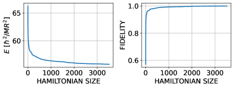
Figure 10: Ground state energy (left) and fidelity (right) for $N=6$ particles and interaction strength $gN=18\hbar^{2}/M$ as a function of order of Hamiltonian matrix (basis size).

To conclude, we found that our results are numerically robust. In fact, in the weakly-interacting limit studied in this manuscript, the many-body states are spanned by just a few Fock states.

References

- Kulish et al. [1976] P. P. Kulish, S. V. Manakov, and L. D. Faddeev, Comparison of the exact quantum and quasiclassical results for a nonlinear schrödinger equation, Theoretical and Mathematical Physics 28, 615 (1976).
- Ishikawa and Takayama [1980] M. Ishikawa and H. Takayama, Solitons in a one-dimensional bose system with the repulsive delta-function interaction, Journal of the Physical Society of Japan 49, 1242 (1980), https://doi.org/10.1143/JPSJ.49.1242 .
- Lieb [1963] E. H. Lieb, Exact analysis of an interacting bose gas. ii. the excitation spectrum, Phys. Rev. 130, 1616 (1963).
- Lieb and Liniger [1963] E. H. Lieb and W. Liniger, Exact analysis of an interacting bose gas. i. the general solution and the ground state, Phys. Rev. 130, 1605 (1963).
- Mottelson [1999] B. Mottelson, Yrast spectra of weakly interacting bose-einstein condensates, Phys. Rev. Lett. 83, 2695 (1999).
- Sato et al. [2012] J. Sato, R. Kanamoto, E. Kaminishi, and T. Deguchi, Exact relaxation dynamics of a localized many-body state in the 1d bose gas, Phys. Rev. Lett. 108, 110401 (2012).
- Syrwid and Sacha [2015a] A. Syrwid and K. Sacha, Lieb-liniger model: Emergence of dark solitons in the course of measurements of particle positions, Physical Review A 92, 032110 (2015a).
- Syrwid et al. [2016] A. Syrwid, M. Brewczyk, M. Gajda, and K. Sacha, Single-shot simulations of dynamics of quantum dark solitons, Physical Review A 94, 023623 (2016).
- Golletz et al. [2020] W. Golletz, W. Górecki, R. Ołdziejewski, and K. Pawłowski, Dark solitons revealed in lieb-liniger eigenstates, Phys. Rev. Res. 2, 033368 (2020).
- Muñoz Mateo et al. [2019] A. Muñoz Mateo, V. Delgado, M. Guilleumas, R. Mayol, and J. Brand, Nonlinear waves of bose-einstein condensates in rotating ring-lattice potentials, Phys. Rev. A 99, 023630 (2019).
- Kaminishi et al. [2020] E. Kaminishi, T. Mori, and S. Miyashita, Construction of quantum dark soliton in one-dimensional Bose gas, J. Phys. B: At. Mol. Opt. Phys. 53, 095302 (2020).
- Kanamoto et al. [2008] R. Kanamoto, L. D. Carr, and M. Ueda, Topological winding and unwinding in metastable bose-einstein condensates, Phys. Rev. Lett. 100, 060401 (2008).
- Kaminishi et al. [2011] E. Kaminishi, R. Kanamoto, J. Sato, and T. Deguchi, Exact yrast spectra of cold atoms on a ring, Phys. Rev. A 83, 031601 (2011).
- Fialko et al. [2012] O. Fialko, M.-C. Delattre, J. Brand, and A. R. Kolovsky, Nucleation in finite topological systems during continuous metastable quantum phase transitions, Phys. Rev. Lett. 108, 250402 (2012).
- Dziarmaga and Sacha [2002] J. Dziarmaga and K. Sacha, Depletion of the dark soliton: The anomalous mode of the bogoliubov theory, Phys. Rev. A 66, 043620 (2002).
- Madison et al. [2000] K. W. Madison, F. Chevy, W. Wohlleben, and J. Dalibard, Vortex formation in a stirred bose-einstein condensate, Phys. Rev. Lett. 84, 806 (2000).
- Coddington et al. [2004] I. Coddington, P. C. Haljan, P. Engels, V. Schweikhard, S. Tung, and E. A. Cornell, Experimental studies of equilibrium vortex properties in a bose-condensed gas, Phys. Rev. A 70, 063607 (2004).
- Abo-Shaeer et al. [2002] J. R. Abo-Shaeer, C. Raman, and W. Ketterle, Formation and decay of vortex lattices in bose-einstein condensates at finite temperatures, Phys. Rev. Lett. 88, 070409 (2002).
- Engels et al. [2002] P. Engels, I. Coddington, P. C. Haljan, and E. A. Cornell, Nonequilibrium effects of anisotropic compression applied to vortex lattices in bose-einstein condensates, Phys. Rev. Lett. 89, 100403 (2002).
- Henn et al. [2009] E. A. L. Henn, J. A. Seman, G. Roati, K. M. F. Magalhães, and V. S. Bagnato, Emergence of turbulence in an oscillating bose-einstein condensate, Phys. Rev. Lett. 103, 045301 (2009).
- Hadzibabic et al. [2006] Z. Hadzibabic, P. Krüger, M. Cheneau, B. Battelier, and J. Dalibard, Berezinskii–Kosterlitz–Thouless crossover in a trapped atomic gas, Nature 441, 1118 (2006).
- Verhelst and Tempere [2017] N. Verhelst and J. Tempere, Vortex structures in ultra-cold atomic gases, in Vortex Dynamics and Optical Vortices, edited by H. P. de Tejada (IntechOpen, Rijeka, 2017) Chap. 1.
- Kadau et al. [2016] H. Kadau, M. Schmitt, M. Wenzel, C. Wink, T. Maier, I. Ferrier-Barbut, and T. Pfau, Observing the rosensweig instability of a quantum ferrofluid, Nature 530, 194–197 (2016).
- Petrov [2015] D. S. Petrov, Quantum mechanical stabilization of a collapsing bose-bose mixture, Phys. Rev. Lett. 115, 155302 (2015).
- Castin [2001] Y. Castin, Bose-Einstein condensates in atomic gases: simple theoretical results, arXiv /10.48550/arXiv.cond-mat/0105058 (2001), cond-mat/0105058 .
- Castin [2002] Y. Castin, Bose-Einstein Condensates in Atomic Gases: Simple Theoretical Results, in Coherent atomic matter waves (Springer, Berlin, Germany, 2002) pp. 1–136.
- Castin and Dum [1998] Y. Castin and R. Dum, Low-temperature bose-einstein condensates in time-dependent traps: Beyond the symmetry-breaking approach, Phys. Rev. A 57, 3008 (1998).
- Caroli et al. [1964] C. Caroli, P. G. De Gennes, and J. Matricon, Bound Fermion states on a vortex line in a type II superconductor, Physics Letters 9, 307 (1964).
- Dziarmaga et al. [2003a] J. Dziarmaga, Z. P. Karkuszewski, and K. Sacha, Images of the dark soliton in a depleted condensate, J. Phys. B: At. Mol. Opt. Phys. 36, 1217 (2003a).
- Javanainen and Yoo [1996a] J. Javanainen and S. M. Yoo, Quantum phase of a bose-einstein condensate with an arbitrary number of atoms, Phys. Rev. Lett. 76, 161 (1996a).
- Note [1] See Supplemental Material.
- [32] S. Albeverio, F. Gesztesy, R. Høegh-Krohn, and H. Holden, Solvable Models in Quantum Mechanics (Springer, Berlin, Germany).
- Mead and Godines [1991] L. R. Mead and J. Godines, An analytical example of renormalization in two-dimensional quantum mechanics, Am. J. Phys. 59, 935 (1991).
- Mora and Castin [2003] C. Mora and Y. Castin, Extension of bogoliubov theory to quasicondensates, Phys. Rev. A 67, 053615 (2003).
- Ołdziejewski et al. [2018a] R. Ołdziejewski, W. Górecki, K. Pawłowski, and K. Rzążewski, Many-body solitonlike states of the bosonic ideal gas, Phys. Rev. A 97, 063617 (2018a).
- Dziarmaga et al. [2003b] J. Dziarmaga, Z. P. Karkuszewski, and K. Sacha, Images of the dark soliton in a depleted condensate, Journal of Physics B: Atomic, Molecular and Optical Physics 36, 1217–1229 (2003b).
- Syrwid and Sacha [2015b] A. Syrwid and K. Sacha, Lieb-liniger model: Emergence of dark solitons in the course of measurements of particle positions, Phys. Rev. A 92, 032110 (2015b).
- Javanainen and Yoo [1996b] J. Javanainen and S. M. Yoo, Quantum phase of a bose-einstein condensate with an arbitrary number of atoms, Phys. Rev. Lett. 76, 161 (1996b).
- Kanamoto et al. [2010] R. Kanamoto, L. D. Carr, and M. Ueda, Metastable quantum phase transitions in a periodic one-dimensional bose gas. ii. many-body theory, Phys. Rev. A 81, 023625 (2010).
- Kosterlitz and Thouless [1973] J. M. Kosterlitz and D. J. Thouless, Ordering, metastability and phase transitions in two-dimensional systems, J. Phys. C: Solid State Phys. 6, 1181 (1973).
- Ołdziejewski et al. [2018b] R. Ołdziejewski, W. Górecki, K. Pawłowski, and K. Rzążewski, Many-body solitonlike states of the bosonic ideal gas, Phys. Rev. A 97, 063617 (2018b).
- Sato et al. [2016] J. Sato, R. Kanamoto, E. Kaminishi, and T. Deguchi, Quantum states of dark solitons in the 1d bose gas, New Journal of Physics 18, 075008 (2016).
- Castin and Herzog [2001] Y. Castin and C. Herzog, Bose-Einstein condensates in symmetry breaking states, Comptes Rendus de l’Académie des Sciences - Series IV - Physics 2, 419 (2001).
- Busch et al. [1998] T. Busch, B.-G. Englert, K. Rzażewski, and M. Wilkens, Two Cold Atoms in a Harmonic Trap, Found. Phys. 28, 549 (1998).