Information-Theoretic Measures on Lattices for High-Order Interactions
Abstract
Traditional models reliant solely on pairwise associations often prove insufficient in capturing the complex statistical structure inherent in multivariate data. Yet existing methods for identifying information shared among groups of variables are often intractable; asymmetric around a target variable; or unable to consider all factorisations of the joint probability distribution. Here, we present a framework that systematically derives high-order measures using lattice and operator function pairs, whereby the lattice captures the algebraic relational structure of the variables and the operator function computes measures over the lattice. We show that many existing information-theoretic high-order measures can be derived by using divergences as operator functions on sublattices of the partition lattice, thus preventing the accurate quantification of all interactions for . Similarly, we show that using the KL divergence as the operator function also leads to unwanted cancellation of interactions for . To characterise all interactions among variables, we introduce the Streitberg information defined on the full partition lattice using generalisations of the KL divergence as operator functions. We validate our results numerically on synthetic data, and illustrate the use of the Streitberg information through applications to stock market returns and neural electrophysiology data.
1 Introduction
Although networks are commonly used as standard descriptions for complex real-world systems, they are inherently restricted to capturing and representing pairwise interactions between units or nodes [1]. Many real-world systems are better characterised by high-order interactions involving groups of three or more units [2, 3, 4, 5]. Yet direct measurements of such group interactions are rarely available, necessitating approaches to reconstruct the systems’ underlying interactions and mechanisms from observed multivariate data [5, 6, 7, 8].
Information theory provides a powerful quantitative framework to dissect complex interactions by detecting high-order interactions with a solid probabilistic basis and the capacity to relate statistical structure to function [9]. Early metrics such as interaction information [10] or co-information [11] began to address these high-order interactions. However, those formulations only consider a subset of the factorisations of the joint probability distribution, thus limiting their scope [12, 13]. More recently, the connected information attempted to capture interactions among variables by considering their maximum entropy states [14]. Yet, its practical application to real-world data is hampered by the computational difficulties in constructing the maximum entropy distributions [15]. One of the more prevalent measures, Partial Information Decomposition (PID), offers a breakdown of high-order interaction into information atoms [16]. While PID provides a detailed insight into how information is shared among variables, it becomes computationally infeasible for and exhibits asymmetry among variables. The increasing interest in detecting high-order interactions in data and the limitations of existing tools underscore the need for more practical and comprehensive information-theoretic measures that can handle systematically and effectively all factorisations of the joint probability distribution.
Here, we develop a framework that systematically formalises high-order information-theoretic measures using lattice theory. By leveraging lattice embeddings and isomorphisms, we demonstrate that various existing information-theoretic measures can be derived from sublattices of the partition lattice, with a divergence function applied to each element within these lattices. Using the complete partition lattice, we propose a novel information measure, the Streitberg Information, as defined in Equation (6). This measure accounts for all factorisations of the joint probability distribution of variables, vanishing when a lower-order factorisation is present. We also demonstrate that using Kullback-Leibler (KL) as a divergence function collapses lattice substructures, resulting in undesired, non-trivial equivalence of measures derived from different sublattices. To preserve the desired vanishing property of the partition lattice, we formulate the Streitberg information using a generalisation of the KL divergence, the Tsallis-Alpha divergence, and develop its non-parametric consistent estimator using a -nearest-neighbours method. Finally, we present numerical validations of the Streitberg information on synthetic data, followed by applications to real-world financial and neural electrophysiology data.
2 Information-theoretic measures of interaction
In information theory, given two random variables, and , the amount of information provided about one of the variables given the value of the other can be quantified by the mutual information
where is the joint entropy of a set of random variables. The mutual information vanishes if and only if the two variables are independent () [17].
The generalisation of mutual information to encompass the dependencies among a set of random variables is not trivial. The simplest way to quantify the amount of information shared among variables is total correlation (TC) [18]:
| (1) |
which vanishes if and only if the variables are jointly independent. Yet fails to provide any details about the exact form of the interactions, i.e., whether it can be explained by the sum of low-order interactions [19, 14]. An alternative extension of mutual information is the interaction information (II) [10] which captures the high-order information in a system of variables through the inclusion-exclusion principle:
| (2) |
where the sum extends over the power set of all subsets of and denotes the cardinality of the set. Although has been widely used, its interpretation when equal to zero is not clear [12]. Below we show that this is because some of the non-trivial high-order terms are decomposed into a sum of lower order terms via KL-divergence (Section 4). We also show that, although seemingly distinct, these generalisations of mutual information to high-orders actually belong to the same family of information-theoretic measures when formalised through lattice theory (Section 3).
3 Lattice theory
To see how different information-theoretic measures (e.g.,those in Section 2) can be systematically generated from different lattices, we provide a few relevant concepts and results from lattice theory.
A partially ordered set (poset) defined on the set with an order is a lattice (denoted by ) if the meet (least upper bound) and the join (greatest lower bound) exist and are contained in for all . The maximum element and the minimum element of are denoted as and , respectively. A subset of closed under and of forms a sublattice (denoted ) of . Let be a real-valued function and let be the sum function of over the interval . Then we have the following relationships, known as the Möbius inversion theorem [20]:
| (3) |
where the partial order is encoded by the Zeta matrix, with if and 0 otherwise. Its inverse is the Möbius matrix with elements . Clearly, a measure derived by Möbius inversion depends on both the structure of the lattice and the choice of (or ); Hence the Möbius inversion on the same poset with different operator functions can lead to different measures. Conversely, in Proposition 1 we show a non-trivial case where different lattices with the same operator function lead to the same (information-theoretic) measure through Möbius inversion.
These links can be understood through lattice homomorphisms [21]. A homomorphism is a map of the lattice into the lattice which satisfies
A one-to-one homomorphism is also called an embedding. If is a bijection, then is an isomorphism (denoted ). Below we show how lattice homomorphisms lead to insights into the relationships between high-order information-theoretic measures.
Definition 1 (Chain).
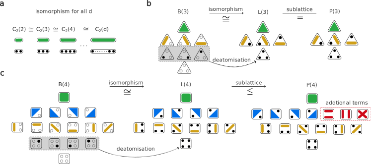
A lattice with elements is a chain, denoted , if or for all . The length of is . See Fig. 1a.
In particular, the two-element chain consists only of elements and with Möbius inversion
| (4) |
If we make equal to the Kullback–Leibler (KL) divergence with respect to , where is the probability function, we trivially retrieve the total correlation (1):
| (5) |
Next, the Boolean lattice (with inclusion partial order) [22] is a natural choice to devise high-order information-theoretic measures as classical information is measured in binary unit bits.
Definition 2 (Boolean lattice).
A lattice is distributive if . A lattice is complemented if there exists such that and . A complemented distributive lattice is a Boolean lattice.
The Boolean lattice is isomorphic to the subset lattice (the powerset of a set ordered by inclusion) and can be used to derive the inclusion-exclusion principle using the Möbius inversion
It then easily follows that using as operator function (as defined for in Eq. (5)) on the Boolean lattice leads to in Eq. (2).
The above lattices are particular embeddings of the partition lattice.
Definition 3 (Partition lattice).
Let denote the set of all partitions of where a partition is a collection of non-empty, pairwise disjoint subsets (blocks) that cover . The partition lattice is defined on the set with the refinement ordering, i.e. for , means every block of is contained in a block of .
The Möbius inversion on the partition lattice, given by
is instrumental to define statistical measures, such as the Lancaster interaction [23], Streitberg interaction [24, 25], and mixed cumulants [26, 27, 28].
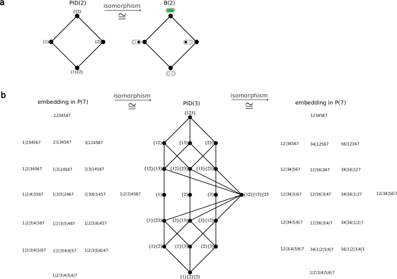
The two-element chain is a sublattice of the partition lattice, , consisting of its minimal and maximal elements, and the chain sublattices for all are isomorphic (Figure 1a). Hence the -induced measure only measures the difference between the joint behaviour of variables and the sum of their individual marginal effects.
Another sublattice of the partition lattice, where partitions contain at most one non-singleton block, is denoted here as the Lancaster lattice (Figure 1b,c).
Lemma 1.
is isomorphic to with the exclusion of singleton elements (deatomisation).
For a proof, see Supplementary Section A.2. As a consequence, -based measures can also be generated from , a sublattice of , e.g., the computation of the Lancaster interaction [23, 25].
Remark (Simplicial complexes): A popular representation of high-order systems is through simplicial complexes [29]. The elements in a ()-simplex with inclusion ordering form a lattice isomorphic to . Furthermore, the boundary matrices of a ()-simplex appear as block submatrices in the Zeta matrix and the Möbius matrix of (see Supplementary Section C).
4 Streitberg information
It is then natural to define an information-theoretic measure based on the Möbius inversion of the full partition lattice with operator function given by a divergence function.
Definition 4.
The Streitberg information is defined as:
| (6) |
where is the corresponding factorisation with respect to , and is a well-defined divergence function.
Similarly, one can define the Lancaster information:
| (7) |
where are the partitions with at most one non-singleton block.
If we choose as the KL divergence as in Eq. (5), then interaction information, Lancaster information and Streitberg information prove to be equivalent. This holds despite these measures being derived from Möbius inversions on distinct lattices.
Proposition 1.
When is the KL divergence,
| (8) |
Proof: The first equality can be proved by counting the number of double-counted marginals due to the KL formalisation. For the second equality, it suffices to show that the KL divergence associated with the non-singleton partitions (except ) vanish. We prove this in three ways in Section A.1 in the SI using (i) the information geometry of KL divergence, (ii) interval lattice, and (iii) the relationship between Lancaster information and Streitberg information.
The equivalence of Möbius functions for different lattices under KL divergence in Eq. (8) implies that certain interaction terms are ignored when KL is chosen. This motivates our exploring alternative divergences that exhibit different information geometries. Here, we consider Tsallis-Alpha divergence [30], a classic generalisation of the KL divergence:
Definition 5 (Tsallis-Alpha divergence).
| (9) |
The Tsallis-Alpha divergence has a wide range of applications in machine learning, including variational inference [31], multiclass logistic regression [32] and image classification [33]. This divergence is uniquely characterised by the parameter : it reduces to the KL divergence when , to the Hellinger distance when [34], and to the distance when [35]. The Tsallis-Alpha divergence is equivalent to the Amari-Alpha divergence up to a substitution of [36].
Crucially, only decomposes into lower order terms when , i.e., when it becomes KL divergence [37, 38]. As a result, vanishes if the joint distribution can be factorised in any way whereas vanishes if the factorisation contains at least one singleton block (Figure 3a-b). To take full advantage of the partition lattice, our focus below is with Tsallis-Alpha divergence.
Recursiveness
Thus far, we have focused on the Möbius function for various lattices and operator functions, treating its counterpart, the Zeta function, primarily as an intermediate tool. However, the Zeta function leads to a recursive definition of high-order measures. Indeed, the expressions of and can be inverted to express the divergence as a sum of s and s using the relationship in Equation (3). By rearranging the Zeta functions (see Supplementary Section A.3), we obtain
Lemma 2.
| (10) |
Hence the Zeta functions of and can be seen as attempts to recursively decompose the divergence between the joint distribution and the product of marginals. This formulation gives an intuitive interpretation when is zero: the dependence in the -order system can be completely explained by the lower order terms. It also follows that the sign of and depends on the difference between the and the sum of the respective low-order information.
Remark: The generalised high-order information on the partition can be defined using the interval lattice , e.g., . This is always zero when due to KL decomposition hence the equivalence in Proposition 1. See Supplementary Section B for more details.
Remark: The recursiveness property underpins the definition of connected information, where it was used without explicit relation to lattice theory [14]. The terms in the connected information are elements of the powerset of , making it directly comparable to - and - induced information-theoretic measures. A significant limitation of connected information is that it lacks an analytical solution; it requires the computation of the maximal entropy distribution for all elements in the powerset, thus making it less desirable than defined on the complete partition lattice.
Symmetry
Both and are symmetric, meaning that they are invariant under permutation of the variables. This contrasts with some information-theoretic measures such as PID that are directed, i.e., they partition the variables into a source set and a target set. In complex multivariate systems, computing a directed measure requires either looping through all the existing variables or constructing a justifiable target. Both approaches can be challenging or sometimes even unfeasible. Moreover, the decomposed information atoms are target-specific and thus insufficient for a comprehensive description of the relationships among variables.
Emergence
A non-zero value of indicates the presence of -order interaction. In particular, we say this is an emergent high-order interaction [39] if for all , i.e. there are no lower order interactions. The high-order interaction can be explained solely by the dependence among variables as the only remaining term is .
Estimation of the measure
In many real-world scenarios, the distribution function of the data often remains unknown, making it impossible to directly compute information-theoretic measures. This limitation necessitates non-parametric estimators that can reliably approximate the true values of these measures. Here, we consider asymptotically unbiased estimators based on the -consistent estimation of Tsallis-Alpha divergence as proposed by Poczos et al. [40] (implemented using python package ITE [41]). With this approach, we avoid direct density estimation by estimating the divergences using -nearest-neighbour statistics. The resulting estimators are a linear sum of the divergences and hence consistent by Slutsky’s theorem [42].
Notice in Eq. (6) that each divergence term consists of a factorisation and its respective complete factorisation. Any factorisations that involve singletons will naturally cancel with the singletons in the complete factorisation, e.g., becomes and the cancellation makes this a 2- instead of a 4-dimensional kNN problem, leading to a more efficient computation (see Section I). As a result, summing over all partitions reduces to sum over the powerset and the partitions with no singletons due to the cancellation of the singletons. To approximate the distributions of the complete factorisation, we permute the realisations of each variables randomly to break any possible dependence among the variables, e.g., the realisations from are generated by randomly permuting the realisation of from .
5 Synthetic experiments
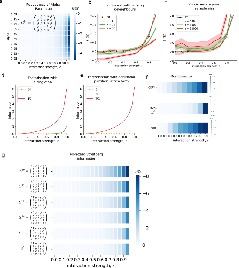
We first validate the Streitberg information using synthetic multivariate Gaussian (MVG) data (with zero mean) with ground truth interactions (analytical solution of MVG in Section D in the SI), and then investigate the accuracy of the kNN-based nonparametric estimation of the measure. Since Lancaster information and Streitberg information diverge for (Streitberg vanishes given any factorisation of the joint distribution while Lancaster does not due to the additional terms in the partition lattice shown in Figure 1c) we show results for . Note that the conclusions from the below experiments also hold for and are shown in Supplementary Section E (Figures 9& 10).
Alpha parameter
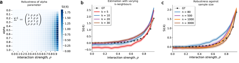
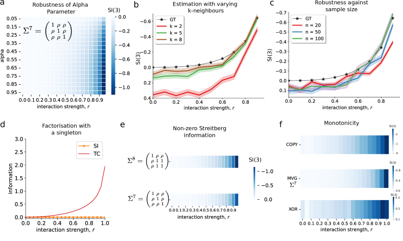
We begin by exploring the behaviour of as we vary the parameter using a MVG with variance where defines the interaction strength between variables (Figure 2a). We find varying does not much change the relationship with , highlighting the robustness of . With the is most sensitive to changes in the interaction strength and will be fixed for the below analyses.
Estimation accuracy
To assess the robustness of SI, we varied (i) the number of neighbours for kNN-based density estimation and (ii) the number of samples. First, we generated realisations of a MVG with covariance and vary the value of . Even with as few as neighbours, the estimation of ground truth is reasonably accurate, albeit the estimation errors when are larger for smaller (Figure 2b). Next, we fixed and varied the number of samples . The estimations are relatively accurate even with only and the errors at both limits of the interaction strength are negligible. Increasing naturally improves estimation at all interaction strengths (Figure 2c).
Vanishing condition
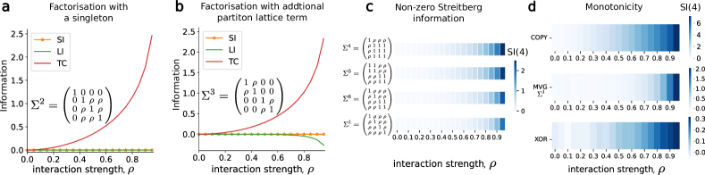
Next, we computed , and for varying analytical factorisations of the joint probability distribution: (i) where , and (ii) where . We would expect a well-behaved high-order information measure to stay at zero when a partial factorisation is present. As expected, fails to capture either partial factorisation of the joint distribution, whilst is only able to detect the factorisation consisting of singletons. On the other hand, is able to detect both factorisations (Figure 3a-b).
Interpretation
The experiments above validate the vanishing condition of . Now, we illustrate the interpretation of when it is non-zero. We define four different MVGs using the below covariance matrices , , and in Figure 3c which are equivalent when tends to 1 and represent block matrices with factorisable distributions when . We first note that Streitberg information increases more rapidly when the covariance matrix contains more independent sub-blocks (when ) in Figure 3c. For covariance matrices with the same number of independent sub-blocks - such as MVG with and - the latter increases more slowly. This difference can be explained by the structure of the probability distributions: pulling out one singleton from creates two new singletons, whereas doing the same from results in at most one new singleton. Therefore the MVG with is more amenable to further factorisation. This suggests that a larger captures a lower likelihood of factorisation, pointing to stronger dependency ties within the variable set.
Monotonicity
Finally, we investigate the monotonicity of using data sets constructed using an XOR gate, a COPY gate and MVG. We generate samples of . For the XOR gate, we set and . For the COPY gate, we set , , . We then gradually increase the interaction proportion, . The MVG is generated with covariance matrix . We find that increases monotonically with interaction strength in all three examples (Figure 3d). By construction, the XOR data set does not contain pairwise or 3-way interactions, and the 4-way interaction becomes more significant as approaches 1. Breaking the 4-way interaction makes all the variables singletons. In contrast, the COPY and MVG data sets contain pairwise, 3-way and 4-way interactions when and are non-zero. In comparison to MVG, the COPY data set contains stronger interactions since the variables are eventually identical (), and thus the magnitude of is greater than MVG.
6 Real-world applications
Finally, we exemplify Streitberg information on two real-world datasets in finance and neuroscience.
Interactions in stock market returns
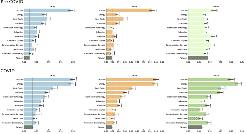
While traditional portfolio optimisation frameworks, which rely on limiting the covariance of investments [43], provide valuable insights into risk and return, they often overlook high-order interactions among stocks. Here, we compute the Streitberg information between stocks in the S&P 500 using their daily returns (assumed as [44]) from 4 Jan 2010 to 24 Apr 2024. For comparison, we computed both the intra- and inter-sector pairwise, 3-, and 4-way Streitberg information.
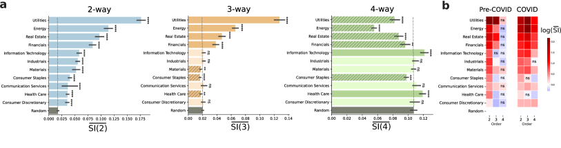
As expected, results in Figure 4a shows that intra-sector pairwise interactions are significantly stronger than inter-sector (gray bar) across all sectors owing to, e.g., shared economic drivers or supply chain interdependencies. At 3-way we observe variation across sectors; sectors like Utilities which are heavily regulated exhibited increasing 3-way interactions, whilst sectors such as Health Care which are more diverse (including pharma companies, biotech firms and healthcare providers) displayed less 3-way interactions. We see further differences at 4-way Streitberg information. For example, the energy sector which is primarily driven by commodity prices, geopolitical events and regulations, had less 4-way interactions. On the other hand, Information Technology, a sector that is characterised by rapid innovation and interdependent product ecosystems, displayed more 4-way interactions (see Section F for more details).
We further computed the Streitberg information before and after 2 Jan 2020 to understand the impact of COVID on the interdependencies between stocks (Figure 4b). Pre-COVID, we found no significant difference in intra-sector 4-way interactions relative to inter-sector, however, since COVID we found that many sectors now show significantly more or less 4-way interactions relative to intra-sector.
Decoding neural spiking data
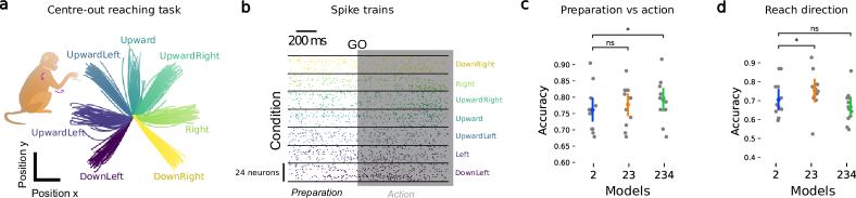
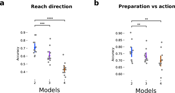
Prior work has found higher-order interactions to play an important role in neuroscientific data [45, 46, 47, 48, 49, 15, 50]. Therefore, next, we asked whether high-order interactions improved decoding of electrophysiological recordings of a monkey performing a delayed centre-out hand-reaching task [51, 52]. In each recording session, the monkey was instructed to perform seven fixed hand movements for a randomly defined number of trials (Figure 5a). The spiking activity for each neuron is recorded using a 24-channel Utah array over a 1.2 second time period (500ms preparation period, 700ms action period, Figure 5b). The spiking data was converted to spiking rates using a Gaussian 20ms kernel. For a given session, we exhaustively computed the 2-, 3- and 4-way Streitberg information of all possible combinations across a set of 12 neurons. This was repeated for each time point of every condition across 12 sessions (more details in Section G).
First, we asked whether high-order interactions were more important during the preparatory stages or motor action. We trained a logistic classifier using varying orders of Streitberg information as features. To avoid overfitting due to the increasing number of features as the order increases, we applied PCA to the -order interaction features and used a constant number of principal components. We found that individually 2-way Streitberg information was most informative, but by also including 3- and 4-way interactions the classification of the two stages was improved (Figure 5c), highlighting their role in neural coding [53]. Again, in the task of decoding reach direction, whilst individually the 2-way Streitberg information is most informative, highlighting the importance of redundancy in neural code [54], we found that a combination of 2- and 3-way Streitberg information is best for decoding reach direction (Figure 5d). The need for 4-way interactions to better predict preparation vs. action, but less useful for decoding reach direction, could be due to the need to integrate information for action planning [45]. In both cases, training a model only using -order interactions led to reduced accuracy (Figure 12).
7 Discussion
In this work, we have established a framework that formulates high-order information-theoretic measures using lattice theory. Through the lens of our framework, we show that well-known information-theoretic measures are readily derived, and we introduce a novel information measure, Streitberg information, that effectively captures all factorisations of the joint distributions.
Our work offers a rigorous and systematic approach for the reconstruction of high-order systems using information-theoretic measures, but has some limitations. While the sign of () is determined by the difference between the total dependence and the sum of the lower order Streitberg information through the recursiveness property, how the sign changes with order remains unexplored.
Despite inherent differences between our measure and PID, whereby our measure is symmetric (not conditioned on a target set), we also show that our framework provides key insights into the formulation of PID via the free distributive lattice (Section H). We note that Streitberg information scales proportional to the Bell number, making it increasingly expensive for large . However, this is considerably more efficient than PID which scales by the Dedekind number [55]. Moreover, the magnitude of Streitberg information is explained in terms of the factorisability of the joint probability distribution, however, the bounds of the measure across alpha remain unclear. Finally, the non-parametric estimation of the Streitberg information assumes that the data is , a strong assumption in many real-world data sets which contain time-series [39]. This leaves several open directions for future work, specifically the investigation of the sign and bounds of Streitberg information across order and alpha; how it can be accurately approximated when the data has temporal dependence; and if the lattice-based framework is helpful in formalising directed information-theoretic measures.
References
- [1] Vito Latora, Vincenzo Nicosia, and Giovanni Russo. Complex networks: principles, methods and applications. Cambridge University Press, 2017.
- [2] Federico Battiston, Giulia Cencetti, Iacopo Iacopini, Vito Latora, Maxime Lucas, Alice Patania, Jean-Gabriel Young, and Giovanni Petri. Networks beyond pairwise interactions: structure and dynamics. Physics Reports, 874:1–92, 2020.
- [3] Alicia Sanchez-Gorostiaga, Djordje Bajić, Melisa L Osborne, Juan F Poyatos, and Alvaro Sanchez. High-order interactions distort the functional landscape of microbial consortia. PLoS Biology, 17(12):e3000550, 2019.
- [4] Jacopo Grilli, György Barabás, Matthew J Michalska-Smith, and Stefano Allesina. Higher-order interactions stabilize dynamics in competitive network models. Nature, 548(7666):210–213, 2017.
- [5] Fernando E Rosas, Pedro AM Mediano, Andrea I Luppi, Thomas F Varley, Joseph T Lizier, Sebastiano Stramaglia, Henrik J Jensen, and Daniele Marinazzo. Disentangling high-order mechanisms and high-order behaviours in complex systems. Nature Physics, 18(5):476–477, 2022.
- [6] Andrea Santoro, Federico Battiston, Giovanni Petri, and Enrico Amico. Higher-order organization of multivariate time series. Nature Physics, 19(2):221–229, 2023.
- [7] Jean-Gabriel Young, Giovanni Petri, and Tiago P Peixoto. Hypergraph reconstruction from network data. Communications Physics, 4(1):135, 2021.
- [8] Huan Wang, Chuang Ma, Han-Shuang Chen, Ying-Cheng Lai, and Hai-Feng Zhang. Full reconstruction of simplicial complexes from binary contagion and ising data. Nature communications, 13(1):3043, 2022.
- [9] Nicholas Timme, Wesley Alford, Benjamin Flecker, and John M Beggs. Synergy, redundancy, and multivariate information measures: an experimentalist’s perspective. Journal of computational neuroscience, 36:119–140, 2014.
- [10] William McGill. Multivariate information transmission. Transactions of the IRE Professional Group on Information Theory, 4(4):93–111, 1954.
- [11] Anthony J Bell. The co-information lattice. In Proceedings of the fifth international workshop on independent component analysis and blind signal separation: ICA, volume 2003, 2003.
- [12] Klaus Krippendorff. Information of interactions in complex systems. International Journal of General Systems, 38(6), 2009.
- [13] Ryan G James and James P Crutchfield. Multivariate dependence beyond shannon information. Entropy, 19(10):531, 2017.
- [14] Elad Schneidman, Susanne Still, Michael J Berry, William Bialek, et al. Network information and connected correlations. Physical review letters, 91(23):238701, 2003.
- [15] Elad Schneidman, William Bialek, and Michael J Berry. Synergy, redundancy, and independence in population codes. Journal of Neuroscience, 23(37):11539–11553, 2003.
- [16] Paul L Williams and Randall D Beer. Nonnegative decomposition of multivariate information. arXiv preprint arXiv:1004.2515, 2010.
- [17] Thomas B Berrett and Richard J Samworth. Nonparametric independence testing via mutual information. Biometrika, 106(3):547–566, 2019.
- [18] Satosi Watanabe. Information theoretical analysis of multivariate correlation. IBM Journal of research and development, 4(1):66–82, 1960.
- [19] Wendell R Garner. Uncertainty and structure as psychological concepts. 1962.
- [20] Edward A Bender and Jay R Goldman. On the applications of möbius inversion in combinatorial analysis. The American Mathematical Monthly, 82(8):789–803, 1975.
- [21] George A Gratzer. Lattice theory: foundation, volume 2. Springer, 2011.
- [22] Martin Aigner. Combinatorial theory. Springer Science & Business Media, 1979.
- [23] Henry O Lancaster. The Chi-Squared Distribution. Wiley, 1969.
- [24] Bernd Streitberg. Lancaster interactions revisited. The Annals of Statistics, pages 1878–1885, 1990.
- [25] Zhaolu Liu, Robert Peach, Pedro AM Mediano, and Mauricio Barahona. Interaction measures, partition lattices and kernel tests for high-order interactions. Advances in neural information processing systems, 36, 2023.
- [26] Terry P Speed. Cumulants and partition lattices. Australian Journal of Statistics, 25(2):378–388, 1983.
- [27] Peter McCullagh. Tensor methods in statistics. Chapman and Hall/CRC, 2018.
- [28] Patric Bonnier, Harald Oberhauser, and Zoltán Szabó. Kernelized cumulants: Beyond kernel mean embeddings. Advances in Neural Information Processing Systems, 36, 2024.
- [29] Ginestra Bianconi. Higher-order networks. Elements in Structure and Dynamics of Complex Networks, 2021.
- [30] Constantino Tsallis. Possible generalization of boltzmann-gibbs statistics. Journal of statistical physics, 52:479–487, 1988.
- [31] Ziyi Wang, Oswin So, Jason Gibson, Bogdan Vlahov, Manan S Gandhi, Guan-Horng Liu, and Evangelos A Theodorou. Variational inference mpc using tsallis divergence. arXiv preprint arXiv:2104.00241, 2021.
- [32] Ehsan Amid, Manfred K Warmuth, and Sriram Srinivasan. Two-temperature logistic regression based on the tsallis divergence. In The 22nd International Conference on Artificial Intelligence and Statistics, pages 2388–2396. PMLR, 2019.
- [33] Marius Vila, Anton Bardera, Miquel Feixas, and Mateu Sbert. Tsallis mutual information for document classification. Entropy, 13(9):1694–1707, 2011.
- [34] Ernst Hellinger. Die orthogonalinvarianten quadratischer formen von unendlichvielen variabelen. W. Fr. Kaestner, 1907.
- [35] Alison L Gibbs and Francis Edward Su. On choosing and bounding probability metrics. International statistical review, 70(3):419–435, 2002.
- [36] S-I Amari. Information geometry on hierarchy of probability distributions. IEEE transactions on information theory, 47(5):1701–1711, 2001.
- [37] Pablo A Morales and Fernando E Rosas. Generalization of the maximum entropy principle for curved statistical manifolds. Physical Review Research, 3(3):033216, 2021.
- [38] Juntao Huang, Wen-An Yong, and Liu Hong. Generalization of the kullback–leibler divergence in the tsallis statistics. Journal of Mathematical Analysis and Applications, 436(1):501–512, 2016.
- [39] Zhaolu Liu, Robert L Peach, Felix Laumann, Sara Vallejo Mengod, and Mauricio Barahona. Kernel-based joint independence tests for multivariate stationary and non-stationary time series. Royal Society Open Science, 10(11):230857, 2023.
- [40] Barnabás Póczos and Jeff Schneider. On the estimation of -divergences. In Proceedings of the Fourteenth International Conference on Artificial Intelligence and Statistics, pages 609–617. JMLR Workshop and Conference Proceedings, 2011.
- [41] Zoltán Szabó. Information theoretical estimators toolbox. The Journal of Machine Learning Research, 15(1):283–287, 2014.
- [42] Kai Lai Chung. A course in probability theory. Academic press, 2001.
- [43] Maximilian AM Vermorken. Gics or icb, how different is similar? Journal of Asset Management, 12:30–44, 2011.
- [44] Mukhtar M Ali and Carmelo Giaccotto. The identical distribution hypothesis for stock market prices—location-and scale-shift alternatives. Journal of the American Statistical Association, 77(377):19–28, 1982.
- [45] Andrea I Luppi, Pedro AM Mediano, Fernando E Rosas, Negin Holland, Tim D Fryer, John T O’Brien, James B Rowe, David K Menon, Daniel Bor, and Emmanuel A Stamatakis. A synergistic core for human brain evolution and cognition. Nature Neuroscience, 25(6):771–782, 2022.
- [46] Charlotte E Luff, Robert Peach, Emma-Jane Mallas, Edward Rhodes, Felix Laumann, Edward S Boyden, David J Sharp, Mauricio Barahona, and Nir Grossman. The neuron mixer and its impact on human brain dynamics. bioRxiv, pages 2023–01, 2023.
- [47] Thomas F Varley, Maria Pope, Joshua Faskowitz, and Olaf Sporns. Multivariate information theory uncovers synergistic subsystems of the human cerebral cortex. Communications biology, 6(1):451, 2023.
- [48] Andrea I Luppi, Fernando E Rosas, Pedro AM Mediano, David K Menon, and Emmanuel A Stamatakis. Information decomposition and the informational architecture of the brain. Trends in Cognitive Sciences, 2024.
- [49] Thomas F Varley, Maria Pope, Maria Grazia Puxeddu, Joshua Faskowitz, and Olaf Sporns. Partial entropy decomposition reveals higher-order structures in human brain activity. arXiv preprint arXiv:2301.05307, 2023.
- [50] Lucas Arbabyazd, Spase Petkoski, Michael Breakspear, Ana Solodkin, Demian Battaglia, and Viktor Jirsa. State-switching and high-order spatiotemporal organization of dynamic functional connectivity are disrupted by alzheimer’s disease. Network Neuroscience, 7(4):1420–1451, 2023.
- [51] Adam Gosztolai, Robert L Peach, Alexis Arnaudon, Mauricio Barahona, and Pierre Vandergheynst. Interpretable statistical representations of neural population dynamics and geometry. arXiv preprint arXiv:2304.03376, 2023.
- [52] Chethan Pandarinath, Daniel J O’Shea, Jasmine Collins, Rafal Jozefowicz, Sergey D Stavisky, Jonathan C Kao, Eric M Trautmann, Matthew T Kaufman, Stephen I Ryu, Leigh R Hochberg, et al. Inferring single-trial neural population dynamics using sequential auto-encoders. Nature methods, 15(10):805–815, 2018.
- [53] Elad Schneidman, Jason L Puchalla, Ronen Segev, Robert A Harris, William Bialek, and Michael J Berry. Synergy from silence in a combinatorial neural code. Journal of Neuroscience, 31(44):15732–15741, 2011.
- [54] Nandakumar S Narayanan, Eyal Y Kimchi, and Mark Laubach. Redundancy and synergy of neuronal ensembles in motor cortex. Journal of Neuroscience, 25(17):4207–4216, 2005.
- [55] Christian Jäkel. A computation of the ninth dedekind number. Journal of Computational Algebra, 6:100006, 2023.
- [56] Edward H Ip, Yuchung J Wang, and Yeong-nan Yeh. Some equivalence results concerning multiplicative lattice decompositions of multivariate densities. Journal of multivariate analysis, 84(2):403–409, 2003.
- [57] Pavel Pudlak and Jiri Tuma. Every finite lattice can be embedded in a finite partition lattice. Algebra Universalis, 10:74–95, 1980.
- [58] Marcel Wild. Tight embedding of modular lattices into partition lattices: progress and program. Algebra Universalis, 79:1–49, 2018.
Appendix A Proofs
A.1 Proof of Proposition 1
Proof.
We first show that the first equality () in Equation 8 holds. In , we sum the divergences over , the partitions with at most one non-singleton block. In each divergence term, the singletons in the probability distribution function corresponding to can be cancelled with the singletons present in the complete factorisation . The resulting divergence is measuring the difference between the non-singleton block and its corresponding complete factorisations, i.e., given where represents the joint distribution of the non-singleton block and are the distributions of the singletons,
The set forms the powerset of elements, hence the terms in apart from the marginals are preserved.
Now the number of terms in with respect to the marginals can be calculated by simplifying the coefficients [56]:
This is the coefficient of the marginals in , therefore .
Next, we prove the second equivalence () in three different ways.
Information geometry
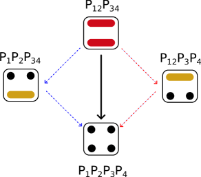
Given a factorisation of variables that consists of only two non-singleton blocks , the KL divergence between itself and can be simplified:
E.g. let ,
The decomposition is shown in Figure 6.
If the number of non-singleton blocks is more than two, one can decompose two blocks at each time and get:
where . This is known as the Pythagorean theorem of KL divergence in information geometry [36]. One can compute the coefficients of the resulting lower order KL divergence terms and will see cancellations occur with the original lower order terms. Instead here we show this can be easily achieved by the information measures defined on the interval lattices.
Interval lattice
The recursiveness of and in Lemma 2 shows that both measures can be expressed by a sum of themselves in lower order. If we take the difference between and we get:
where is the Streitberg information defined on the interval lattice , a sublattice of (for details of the measure on interval lattice, see Section B). Each is expressed by the sum of the KL divergences related to the factorisation of and equals zero due to the Pythagorean theorem above.
Expectation
Finally, we define as the Möbius inversion on with the probability distribution function. Then we take the log of each term in and denote this as . We note that can be constructed by taking the expectation of . By the equivalence proved in Ref. [56], we also get equivalence. ∎
A.2 Proof of Lemma 1
Proof.
One can observe that the structure of the is identical to up to isomorphism except on the second last level on which the singleton elements lie. Two examples for are shown in Figure 1b-c. The length of minus the length of is precisely one and this correspond to the level of singletons which are united together to form in . Excluding these elements leads to the isomorphism. ∎
A.3 Proof of Lemma 2
Proof.
The Zeta function of is:
for all . Moving the lower order sum to the left hand side we recover:
Similarly for . ∎
Appendix B Generalised Streitberg information
The Streitberg information defined on a factorsation with , can be used to assess the factorisability of . We can formulate the generalised Streitberg information using the generalised Streitberg interaction measure proposed in Ref. [25]. Again we first find the Möbius inversion on the interval lattice [27, 21] and apply the divergence function to each term.
Definition 6 (Generalised Streitberg information).
where , are the Möbius coefficients on .
Appendix C Simplicial Complex
We first show how simplicial complex is linked to the Boolean lattice. The definition of a -simplex is a set of +1 vertices , i.e., a 1-simplex is a line, a 2-simplex is a triangle, 3-simplex is a tetrahedron, etc. A simplicial complex is a collection of simplices that satisfy two conditions: (i) if , then all the sub-simplices built from subsets of are also contained in ; and (ii) the non-empty intersection of two simplices is a sub-simplex of both and . One easily realise that the simplicial complex with inclusion ordering is isomorphic to the Boolean lattice.
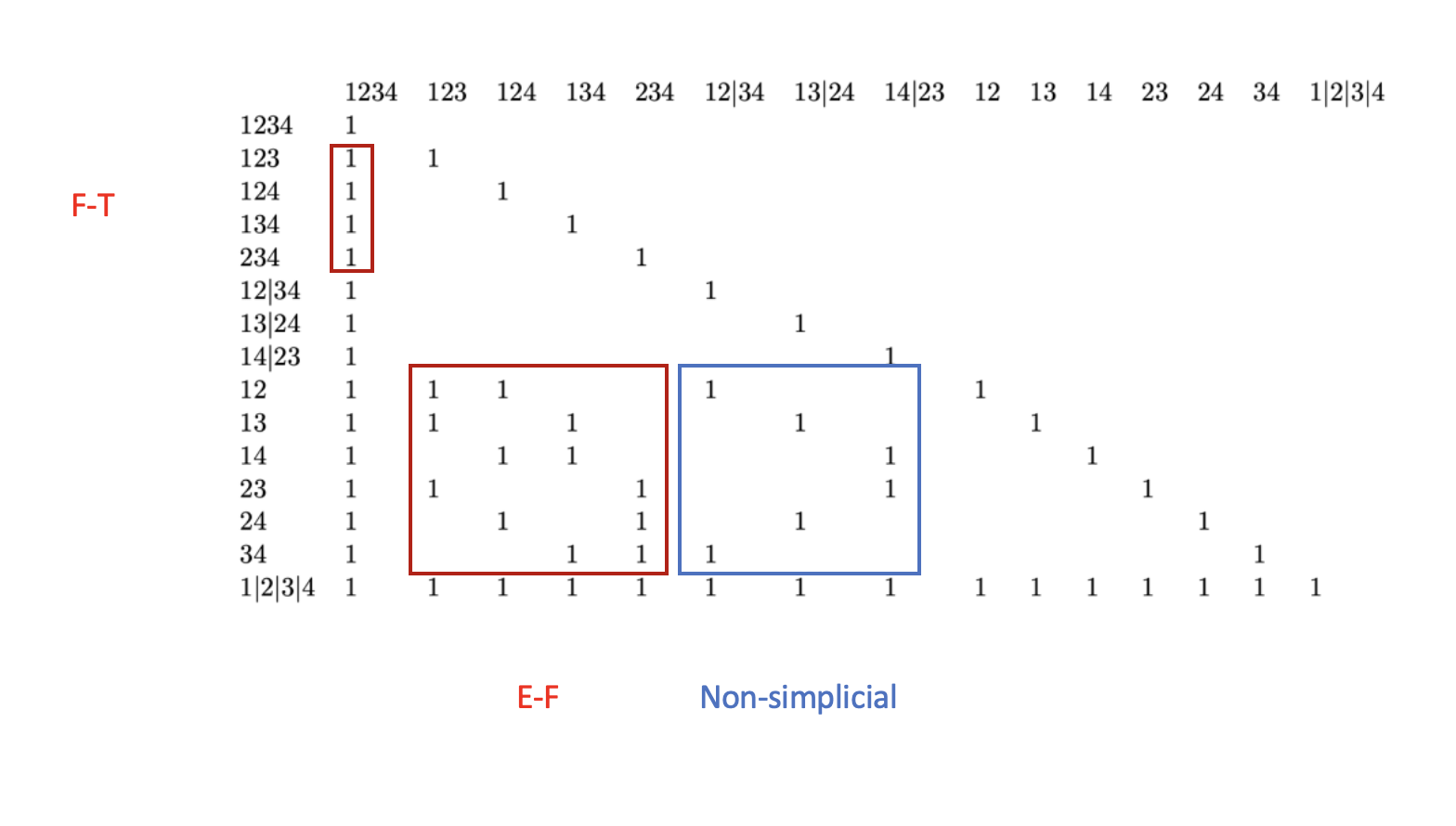
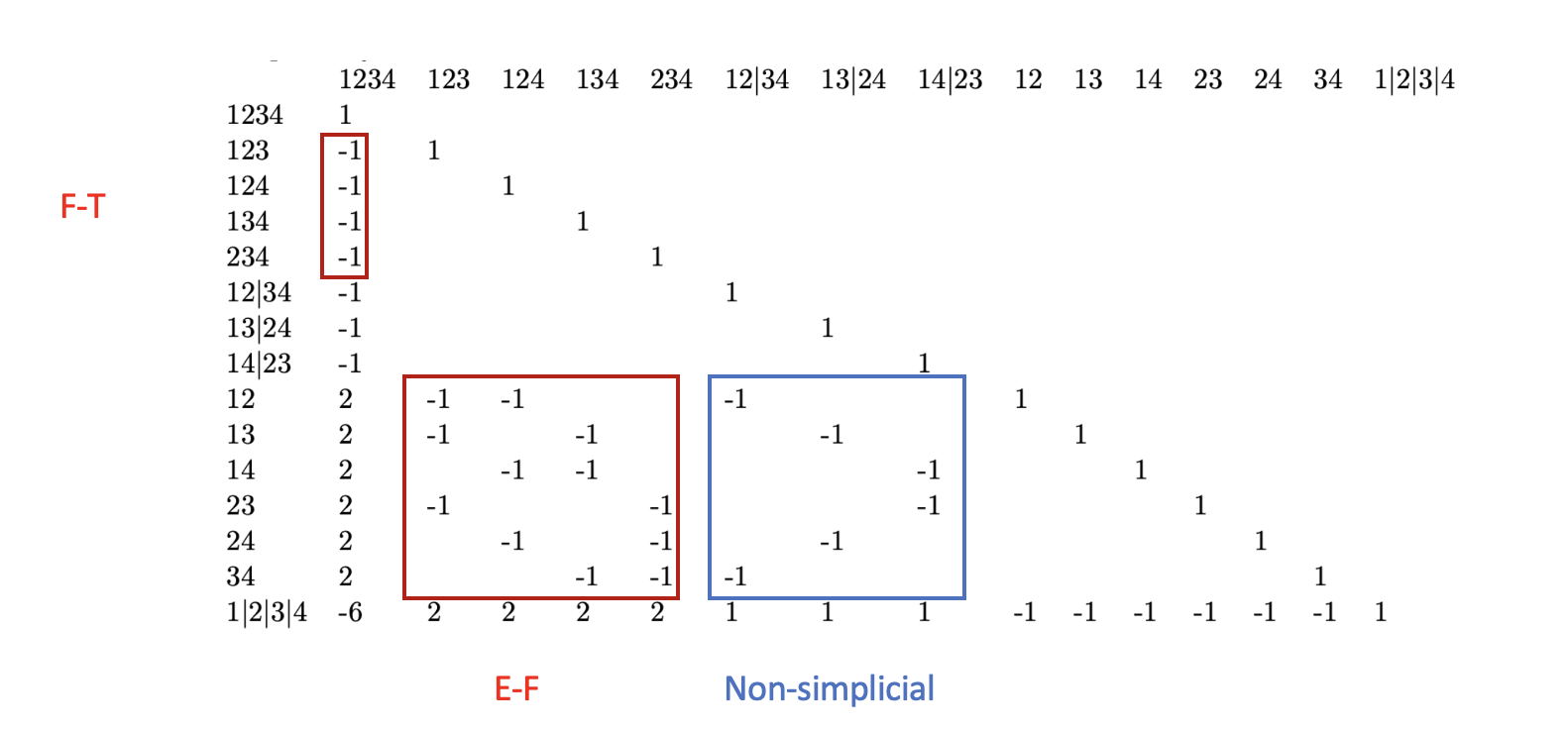
Next we link the simplicial complex to the partition lattice using its boundary operators. Below we have the Zeta matrix in Figure 7 and Möbius matrix in Figure 8 to illustrate that the boundary operators (with no directionality) of (-1)-simplex can be founded as block matrices within them. Simplicial complex does not contain terms consisting of more than one non-singleton block, e.g. which are crucial in the partition lattice to ensure vanishment when .
Appendix D Tsallis-Alpha Divergence for Multivariate Gaussian: Analytical Expression
Following from the analytical solution of Tsallis-Alpha divergence between multivariate Gaussian [40], we further simplify the divergence between the multivariate Gaussian with and its complete factorisation with .
where is the determinant of the matrix. Here is simply the identity matrix in our case, i.e. mean vector is the vector of zero and the covariance matrix has no pairwise dependence and the variances on the diagonal are 1.
Specifically, when , we retrieve the KL divergence and its analytical solution of multivariate Gaussian is
Appendix E Additional synthetic experiments
Appendix F Stock market data
The data is accessed using the following link: https://www.kaggle.com/datasets/andrewmvd/sp-500-stocks.
For a given stock in the S&P 500, we calculate the daily return from 4 Jan 2010 to 24 Apr 2024 as the difference between its closing and opening prices on each day. The returns at different time points are generally assumed as [44]. Next we drop the stocks that have more than 20% of missingness in time and then drop the time points if there is missingness in any stocks. As a result we have 2900 realisations of daily returns of 459 stocks in S&P 500. Each stock belongs to one of the 11 sectors as defined in Global Industry Classification Standard (GICS). We compute the pairwise, 3-, 4-way SI to the sets of stocks that are either taken from within the same sector or sampled at random from the 459 stocks. In each case, we sample 500 sets of regions or take all possible combinations, whichever is lowest.
Appendix G Macaque reaching task data
In the model predicting the preparation and action stages, we use set the time points that correspond to preparation and action to 0 and 1 respectively. In the model decoding the direction of the monkey’s hand movement, we use use ordinal encoding to label the directions from DownLeft to DownRight using the order in Figure 5a. We then train each Logistic classifier (with liblinear solver and L2 penalty) using the 80% of the data and report the model accuracy on the other 20%. The data can be accessed through https://dataverse.harvard.edu/file.xhtml?fileId=6969883&version=11.0.
Appendix H PID embedding
Multivariate information measures are frequently used to measure synergy and redundancy, however, the precise meanings of synergy and redundancy is an ongoing debate. A typical example of synergy is an XOR logic gate whilst a typical example of redundancy is when all the variables are identical. PID offers a direct approach to quantify synergy and redundancy, defining them as distinct information atoms in the mutual information between a target variable and a set of source variables [16]. The entire set of information atoms are formalised by the redundancy lattice (the free distributive lattice without its maximal and minimum elements), with the number of information atoms given by the Dedekind number, which quickly becomes intractable (e.g., 7581 when ; the exact values beyond has yet to be found [55]). To the best of our knowledge, due to the complexity of the free distributive lattice, PID is not currently defined for and will be computationally prohibitive due to the lattice structure and the directed construction.
Notably, it has been shown that every finite lattice can be embedded into a finite partition lattice [57], leading to the following relationship between the free distributive lattice and the partition lattice:
Lemma 3.
A free distributive lattice with length can be embedded into a partition lattice of length where the length of a lattice is if there is a chain in of length and all chains in are of length .
This is a simple result from the tight embedding property of distributive lattices in the partition lattice [58]. In particular, the PID lattice with two variables, excluding empty joins and meets, is isomorphic to the Boolean lattice with two elements (in Figure 13a). Similarly, the PID lattice with three variables can be embedded into a partition lattice with seven elements (two examples shown in Figure 13b).
Appendix I Computational considerations
The kNN-based estimation of the has time complexity where is the number of variables, is the parameter in kNN and is the sample size. The time complexity for estimating can be reduced as the singletons in each partition cancel out with the singletons in the complete factorisation. E.g. when ,
| (11) | ||||
| (12) | ||||
| (13) | ||||
| (14) |
The cancellation of singletons in Equation (14) reduces the complexity from estimating five 3-dimensional (in total 15) to one 3-dimensional and three 2-dimensional (in total 9). Here we fix and and investigate how singleton cancellations reduce the time complexity of and as varies between 2 and 6 shown in Table 1.
| Order | 2 | 3 | 4 | 5 | 6 |
|---|---|---|---|---|---|
We report the computational time in Table 2 for all experiments of Streitberg information using the nonparametric estimation . All experiments carried out on a 2015 iMac with 4 GHz Quad-Core Intel Core i7 processor and 32 GB 1867 MHz DDR3 memory.
| Experiment | Fig.2b | Fig.2c | Fig.3d | Fig.4a | Fig.4b | Fig.5 |
| T ime | 22m35s | 1m28s | 9m54s | 1h26m3s | 50m2s | 5h19m32s |
The code and data used to perform the experiments in the paper are provided in the GitHub repository: https://github.com/neurips2024hoi/nips2024hoi.git.