CNN-JEPA: Self-Supervised Pretraining Convolutional Neural Networks Using Joint Embedding Predictive Architecture

Abstract

Self-supervised learning (SSL) has become an important approach in pretraining large neural networks, enabling unprecedented scaling of model and dataset sizes. While recent advances like I-JEPA have shown promising results for Vision Transformers, adapting such methods to Convolutional Neural Networks (CNNs) presents unique challenges. In this paper, we introduce CNN-JEPA, a novel SSL method that successfully applies the joint embedding predictive architecture approach to CNNs. Our method incorporates a sparse CNN encoder to handle masked inputs, a fully convolutional predictor using depthwise separable convolutions, and an improved masking strategy. We demonstrate that CNN-JEPA outperforms I-JEPA with ViT architectures on ImageNet-100, achieving 73.3% linear top-1 accuracy with a standard ResNet-50 encoder. Compared to other CNN-based SSL methods, CNN-JEPA requires 17-35% less training time for the same number of epochs and approaches the linear and k-NN top-1 accuracies of BYOL, SimCLR, and VICReg. Our approach offers a simpler, more efficient alternative to existing SSL methods for CNNs, requiring minimal augmentations and no separate projector network.

I Introduction

Self-supervised learning (SSL) became an important approach in pretraining large neural networks that allowed to scale model and dataset size to levels previously not possible. It is one of the driving mechanisms behind the recent rapid progress in large-language models. Self-supervised pretraining presents a novel paradigm which aims at learning general representations, rather than learning task-specific features.

In computer, vision designing good self-supervised pretext learning tasks is a challenging problem, with many methods proposed in the literature. One such approach is masked image modeling (MIM), where patches of the input image are masked, and the network is trained to predict the masked patches. Such methods were proposed for Vision Transformers (ViTs) primarily [1], but were also introduced for Convolutional Neural Networks (CNNs) [2, 3]. A more recent, successful approach is I-JEPA [4] (Image Joint Embedding Predictive Architecture) that essentially performs masked image modeling in the latent space by predicting the latent representation of the masked patches from provided context patches. This approach is particularly well-suited for Vision Transformers, which provide good scaling to large datasets and allow for simple implementation of masking.

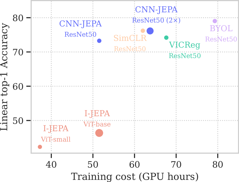
Figure 1: Comparing CNN-JEPA (our method) to I-JEPA [4] and common SSL methods based on Linear top-1 accuracy and Training cost on ImageNet-100. The area of the markers are proportional to the number of parameters in the model.

Despite the growing popularity of Vision Transformers, Convolutional Neural Networks still provide competitive performance on many tasks, and are widely used in practice. They are specifically efficient and provide better performance on small to medium-sized datasets where the inductive biases of CNNs provide an advantage. However, adapting I-JEPA to CNNs is non-trivial, as neither masking nor the prediction from a dense feature map is straightforward. Computing feature maps for a masked input requires masked convolution and careful construction of the mask, that takes the downsampling of the network into account. Predicting masked patches is also challenging because it requires sufficiently large receptive field that is able to predict the latent representation based on provided context. Typical CNNs achieve large receptive fields by stacking many convolutional layers, which can be extensively parameter heavy and computationally expensive for feature maps with high depth.

In this work we propose a novel self-supervised learning method, CNN-JEPA (Convolutional Neural Network-based Joint Embedding Predictive Architecture), that addresses the challenges of adapting I-JEPA to CNNs. The masked image modeling approach proposed Tian et al. [3] uses masked convolutions and masks that are constructed based on the downsampling of the network. We introduce such sparse CNN encoder to I-JEPA to address the challenges of masking. We also introduce a novel, fully convolutional predictor architecture using depthwise separable convolutions that can predict the latent representation of the masked patches with low parameter count and computational cost. Additionally, we improve and simplify the masking strategy of I-JEPA by predicting masked patches as a single region based on the context region as the input for the predictor, instead of using multiple target regions as used by Assran et al. [4]. Our main contributions are:

1. A novel self-supervised learning method, CNN-JEPA, that adapts the successful I-JEPA method to Convolutional Neural Networks.

2. Sparse CNN encoder architecture that can correctly handle masked inputs and produce masked feature maps based on masked CNNs proposed by Tian et al. [3].

3. The introduction of a novel, fully convolutional predictor using depthwise separable convolutions.

4. A masking strategy that follows the downsampling of the network and uses a single target region for the masked prediction task.

Source code supporting the findings of this study is available at https://github.com/kaland313/CNN-JEPA.

II Related Work

Many SSL methods have been proposed in the literature. We propose to categorize the ones that are most relevant to our work into two main groups: instance discriminative and reconstruction-based approaches. Instance discriminative methods, such as BYOL[5], SimCLR[6], and VICReg[7], learn representations by maximizing similarity between augmented views of the same image. These methods employ different mechanisms to avoid trivial solutions, including the use of negative samples, asymmetric architecture, momentum encoder, and regularization.

Reconstruction-based methods primarily rely on masked image modeling pretext tasks, where parts of the input image are masked, and the network is trained to predict the pixels of the masked regions. These methods were initially proposed for Vision Transformers[1], but were also adapted to Convolutional Neural Networks[2, 3]. Earlier works applied other reconstruction-based pretext tasks, such as predicting the color of the image from the grayscale version[8]; however, masked image modeling has shown to be more effective.

Instance discriminative methods learn image-level features that are invariant to the augmentations used to generate views, and aim to capture high-level semantics of the image. On the other hand, these methods rely heavily on hand crafted augmentations and are not trained to capture local details. In contrast, reconstruction-based methods learn more localized features that capture local detail information necessary to solve the reconstruction task; however, their pixel reconstruction objective function might not capture high-level semantics of the image. Assran et al. [4] proposed I-JEPA, a method that combines the benefits of both approaches by performing masked image modeling in the latent space, where the network is trained to predict the latent representation of the masked patches. I-JEPA was primarily designed for Vision Transformers, and adapting it to Convolutional Neural Networks has not been explored in the literature to the best of our knowledge.

III Method

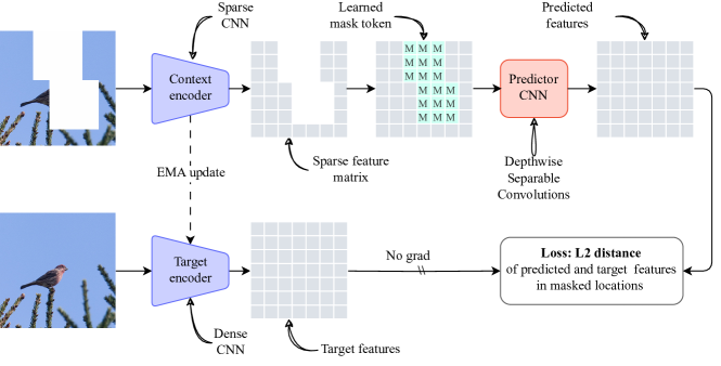
Figure 2: Overview of the CNN-JEPA method. The student and teacher encoders share a common architecture, such as a ResNet-50, with the student encoder using sparse convolutions. The learning objective is to predict the latent representations of masked patches using a predictor, which also trains the student encoder.

III-A CNN-JEPA Algorithm

The overview of the proposed CNN-JEPA algorithm is shown on fig. 2. The proposed method trains an encoder by masking patches of the input image and predicting the latent representation of the masked patches using a predictor. The target latent representations are obtained by a teacher encoder whose weights are updated using the exponential moving average of the student encoder’s weights. We introduce a sparse CNN architecture for the student encoder that can correctly handle masked inputs and produce masked feature maps. For training, we provide the same image to both the student and teacher encoders, with masking applied only to the student encoder’s input. We refer to the masked image and features as the context, based on which the predictor produces the latent representation at the masked locations. Before feeding the masked latent representation to the predictor, masked locations in the student feature maps are filled with a learnable mask token, as proposed by Assran et al. [4]. These feature maps are then passed to a predictor, which is a CNN that predicts the latent representation of the masked patches.

The training objective is to minimize the L2 loss between the predicted latent representations and the target latent representations at the masked locations. Loss is not computed for non-masked patches, using the complement of the context-mask as the mask for the loss computation.

III-B Student and teacher encoder

The student and teacher networks in our proposed method share a common architecture, similarly to other self-supervised learning methods that employ asymmetric student-teacher mechanisms (such as BYOL [5], DINO [9] and I-JEPA [4]). However, a key distinction in our approach is that the student network utilizes sparse convolutions, as introduced by Liu et al. [10] and later employed by Tian et al. [3] for masked image modeling. This sparse convolutional architecture is necessary for handling masked inputs and producing masked feature maps. In practice, we implement sparse convolutions by masking the outputs of standard convolutional layers as detailed in section IV-A. This allows for easily updating the weights of the teacher network based on the student weights.

The teacher network employs standard convolutions. Following Assran et al. [4], the student network is trained using gradient-based optimization techniques, while the weights of the teacher network are updated through an exponential moving average of the student weights. This update mechanism ensures that the teacher network provides stable target representations for the student. We also refer to the student and teacher encoders as context and target encoders, respectively.

III-C Predictor

The predictor in our proposed method operates on feature maps and predicts the latent representation of the masked patches.

Feature maps typically have high depth (e.g., 768 for ConvNeXts [11] and ViT-Base [12], 2048 for ResNet-50 [13]), but low spatial resolution (e.g., 7x7 when using a ResNet-50 on 224x224 images). As the output of the predictor must have the same dimensionality and shape as the feature maps, its outputs also have such depth and spatial size properties. The number of parameters scales quadratically with the depth for convolutional layers that have the same input and output shape. Hence, for high depth, they require a large number of parameters and are computationally expensive. To address this, we propose to use depthwise separable convolutions, which are more parameter efficient and computationally cheaper than standard convolutions. With standard convolutions, the number of parameters in the predictor can easily exceed the number of parameters in the encoder, making the training inefficient, as more resources are spent on the predictor than the encoder. Our use of depthwise separable convolutions helps mitigate this issue, ensuring a more balanced distribution of computational resources between the predictor and the encoder.

III-D Mask token

The masked locations in the student feature maps are filled with a learnable mask token, before passing them to the predictor, similarly to how masked image modeling [1] and I-JEPA [4] uses a mask token. While such use of a mask token is common with vision transformers, SparK [3] also utilizes it for masked auto-encoding with CNNs. In our case, the mask token is a parameter vector with the same dimensionality as the depth of the feature maps and is shared across all masked locations and samples of a minibatch.

III-E Masking

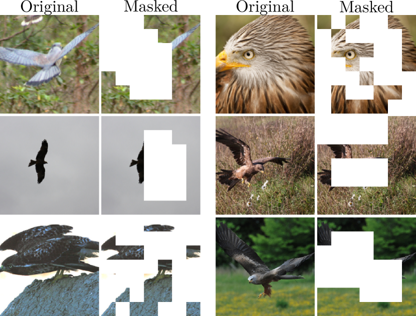
Figure 3: Example masked images, generated using multi-block and random masking strategies. The multi-block approachs masks multiple connected regions in rectangular blocks. Random masking samples patches uniformly from the image up to a given masking ratio. We employ both masking strategies, with a 0.75 probability of using multi-block masks for a given minibatch of images.

In masked image modeling, the most common masking strategy is random masking, where patches are uniformly sampled up to a given masking ratio. I-JEPA [4] introduces the multi-block masking scheme, where blocks of multiple patches are sampled, patches within blocks are masked, while patches outside the blocks form the context from which the predictor predicts the latent representations. I-JEPA presents an empirical study on random, single and multi-block masking and shows that the latter is the most effective by a large margin. We adapt the multi-block masking strategy to CNNs, however we handle the prediction of masked patches differently. While I-JEPA predicts latent features for each block separately, we consider the union of the blocks as the masked region and predict the latent representation of the whole region. For CNNs, the latter approach is simpler to implement and equivalent in terms of learning. The context for the prediction are patches outside any masked patch in both our work and I-JEPA.

When using masked image modeling with CNNs, the mask size is determined by the downsampling of the network. Typically, ResNets and ConvNeXts halve the resolution of feature maps in 5 stages (via pooling) resulting in 32 times downsampling. In order to keep the masking consistent with feature map resolution, we use masks with patch size of $32\times 32$ pixels, which corresponds to $1\times 1$ spatial dimensions (”pixels”) for final feature maps. For images with $224\times 224$ resolution, feature maps have $7\times 7$ spatial dimensions, with matching $7\times 7$ masks of $32\times 32$ pixel patches. For ViTs, the patch size is determined by the patch size of the transformer, which is typically $16\times 16$ or $14\times 14$ pixels.

III-F Comparison to other methods

Thanks to its joint embedding predictive architecture, our method learns patch-level features, which present a good trade-off between image-level and pixel-level features. This approach enables the model to capture more localized features compared to instance discriminative algorithms, while also extracting higher-level features than those obtained using masked image modeling methods.

Compared to common instance discriminative SSL methods one key advantage of our proposed method is its simplicity. It requires minimal handcrafted augmentations, relying only on random resized crop and masking.

Additionally, our approach doesn’t require a separate projector network as opposed to most SSL methods, further simplifying the architecture and reducing computational overhead. Many SSL approaches learn features invariant to diverse augmentations, necessitating a projector network after the encoder. The use of such projector allow the encoder to learn more general features, while the projector learns mapping specific to the loss function and augmentations of the SSL method. Similarly to I-JEPA [4], our approach learns general features without the need for such projector network.

IV Experiments

IV-A Encoder

We conduct experiments using a ResNet-50[13] encoder, for its common use in SSL literature. Sparse convolutions are implemented by zeroing out the outputs of each convolutional layer using a mask appropriately upscaled to the layer’s activation dimensions. While this is computationally inefficient, it is simple to implement and can use standard convolutional layers, which are optimized for many GPU architectures. Using sparse convolutional layers would require a specialized GPU library (e.g., Minkowski Engine [14]), and it would make the implementation of our method more complex and harder to reproduce. Additionally, using standard convolutions simplify the exponential moving average update of the teacher encoder’s weights.

IV-B Predictor

For the predictor, we use 3 depthwise separable convolutional layers with kernel size 3$\times$3, Batch Normalization [15], and ReLU activation. The layers of the predictor follow the pattern: 3$\times$(DepthwiseConv-PointwiseConv-BatchNorm-ReLU). We conduct ablation studies on the predictor architecture and show that this configuration is the most effective.

IV-C Datasets

We conduct experiments on ImageNet-100 and ImageNet-1k [16] datasets. With encoder architectures that downscale by a factor of 32, such as a ResNet-50, the patch size must be at least 32x32 pixels, therefore images must be sufficiently larger than 32x32 pixels to provide meaningful target and context regions for the masked embedding prediction task. Hence, we use 224x224 pixel images from ImageNet-1k and ImageNet-100. Additionally, for these reasons, we do not conduct experiments with lower resolution images and datasets such as CIFAR-10 or STL-10.

IV-D Classification Probes

To evaluate the quality of the learned representations, we use linear and k-nearest neighbor (k-NN) classification probes on top of the encoder’s frozen features. We train the fully connected layer of the linear probe for 90 epochs and report the best top-1 and top-5 accuracies. For k-NN classification, we use the same features and also report top-1 and top-5 accuracies. For both probes, we use minimal augmentations: deterministic resizing and cropping, and normalization. We adapt the hyperparameters of both probes from Lightly [17].

TABLE I: Linear and k-NN top-1 accuracies for different algorithms and backbones on ImageNet-1k and ImageNet-100 datasets. All experiments were limited to 100 epochs for ImageNet-1k and 200 epochs for ImageNet-100.

	Dataset	ImageNet-100		ImageNet-1k
		Linear top-1	k-NN top-1	Linear top-1	k-NN top-1
Backbone [# Paramters]	Algorithm
ResNet-50 [23.5 M]	SimCLR [6]	76.20	67.26	59.81	45.31
	BYOL [5]	79.02	68.20	60.22	45.38
	VICReg [7]	74.18	64.32	59.83	46.82
	CNN-JEPA [Ours]	73.26	59.22	54.23	35.34
ViT-Small [21.6 M]	I-JEPA[4]	42.30	34.84	-	-
ViT-Base [85.7 M]		46.36	31.36	-	-

IV-E Training Details

We use the AdamW optimizer with a constant weight decay of 0.01. A cosine learning rate scheduler with warm-up is employed for 10 epochs, reaching a peak learning rate of 0.01. The per-device batch size is 128 with 4 GPUs, resulting in a total batch size of 512. We update the weights of the teacher encoder using the exponential moving average approach common in other SSL methods [5, 4], with the momentum parameter increasing from 0.996 to 1.0 over the full training period.

Training is conducted for 200 epochs on ImageNet-100 and 100 epochs on ImageNet-1k. All pretraining runs are performed on 4 NVIDIA A100 40GB GPUs on a cluster, with each node having 4 GPUs, 256 GB RAM, and 64 CPU cores. Pretraining on ImageNet-100 for 200 epochs on this hardware takes 13 hours, while pretraining on ImageNet-1k for 100 epochs takes 70 hours.

We utilize PyTorch, PyTorch Lightning [18], and the Lightly [17] SSL library for implementing baselines, probes, and our method. We obtain the I-JEPA ViT results from the official implementation [4].

The cumulative runtime for all experiments in this research is 10 000 hours with an estimated total emission of 1000 kgCO₂eq.

V Results

V-A Comparison to other methods

Our main results are shown in figs. 1 and I. We compare our method to vision transformers trained with I-JEPA and to common SSL methods that were published for CNNs, such as SimCLR, BYOL, and VICReg. Figure 1 shows that on ImageNet-100 our method outperforms I-JEPA with ViT-Small and ViT-Base by a large margin, and achieves 73.3% linear top-1 accuracy with a standard ResNet-50 encoder, a result which is competitive with CNN-based SSL methods. Moreover, our method is computationally more efficient than other CNN-based methods due to the simpler, projector-free architecture and the use of only basic augmentations, requiring 17 to 35% less pretraining hours compared to SimCLR and BYOL respectively. As shown in table I, our method also performs well on ImageNet-1k, achieving a linear top-1 accuracy of 54.23% in 100 epochs.

V-B Masking strategy

TABLE II: Ablation on masking strategies on ImageNet-100.

	Linear	k-NN
Masking strategy	top-1	top-1
Mixed	73.26	56.26
Multi-block	73.02	55.62
Random	57.64	36.64

We experiment with different masking strategies and present our results in table II. Random masking, common in most masked autoencoding methods (e.g. [2, 1, 3]), performs poorly, which is in line with the findings of I-JEPA [4]. The multi-block masking strategy proposed by Bojanowski et al. [4] performs well on convolutional networks as well. Additionally, we propose a mixed masking strategy, where we randomly select between the multi-block and random masking strategies for each minibatch. To primarily use multi-block masking, we choose the probability of using multi-block masking to be 0.75. As shown in table II, the mixed masking strategy performs better than both random and multi-block masking, outperforming the latter by a small margin both on linear and k-NN classification.

V-C Predictor architecture

TABLE III: Ablation on using depthwise separable convolution in the predictor on ImageNet-100.

Predictor	Linear	k-NN	Predictor	Training cost
convolution	top-1	top-1	size [M]	(GPU hours)
Standard	72.64	54.76	12.7 M	62.07
Depthwise separable	73.26	56.26	113 M	51.51

TABLE IV: Predictor depth ablation on ImageNet-100 and ImageNet-1k.

	Predictor	Linear	k-NN	Predictor
Dataset	# layers	top-1	top-1	size [M]
ImageNet-100	1	64.86	51.84	4.2 M
	2	73.22	59.22	8.4 M
	3	73.26	56.26	12.7 M
	4	71.72	53.84	16.9 M
	5	71.14	50.94	21.1 M
	6	69.24	47.68	25.3 M
ImageNet-1k	2	49.78	31.96	8.4 M
	3	54.23	35.00	12.7 M

TABLE V: Predictor kernel size ablation on ImageNet-100.

Predictor	Linear	k-NN	Predictor
kernel size	top-1	top-1	size [M]
3	73.26	56.26	12.7 M
5	73.08	54.88	12.8 M
7	72.44	53.76	12.9 M
9	73.16	53.46	13.1 M

We conduct ablation on the predictor architecture and present the results in tables V, IV and III. Table III clearly shows the benefits of using depthwise separable convolution in the predictor. Depthwise separable convolution not only requires 90% fewer parameters than standard convolution and reduces training time by 17%, but also improves the linear and k-NN top-1 accuracies by 0.62% and 1.5% respectively on ImageNet-100.

The depth of the predictor also has significant impact on pretraining performance. As shown in table IV, two or three layers are optimal, even though such predictors have a smaller receptive field than deeper predictors. On ImageNet-100, linear and k-NN top-1 accuracies indicate different optimal depths; however, on ImageNet-1k, the three-layer predictor provides the highest accuracy by a large margin, 6% and 3% respectively.

Table V shows our results on the predictor’s kernel size. We find that 3x3 kernels provide the highest accuracies; however, the difference between all tested kernel sizes is less than 3%.

VI Conclusions

In this paper, we present CNN-JEPA, a novel self-supervised learning method that successfully adapts I-JEPA to convolutional networks. Our method overcomes the challenges of applying masked inputs to CNNs through the use of a sparse CNN encoder and carefully designed masking strategy. To efficiently handle the joint embedding prediction task, our method utilizes a fully convolutional predictor with depthwise separable convolutions. We demonstrated that CNN-JEPA outperforms I-JEPA with ViT architectures on ImageNet-100 and is competitive with other CNN-based SSL methods on both ImageNet-100 and ImageNet-1k, achieving top-1 linear accuracies of 73.26% and 54.23% respectively. Our proposed mixed masking strategy, combining multi-block and random masking, showed improved performance over either strategy alone. Ablation studies on the predictor architecture revealed the benefits of using depthwise separable convolutions and optimal depth setting for the predictor. CNN-JEPA provides a simpler and more efficient approach to self-supervised learning for CNNs, requiring minimal augmentations and no separate projector network.

References

- [1] K. He, X. Chen, S. Xie, Y. Li, P. Dollár, and R. Girshick, “Masked Autoencoders Are Scalable Vision Learners,” in Proceedings of the IEEE/CVF Conference on Computer Vision and Pattern Recognition, 2022, pp. 16 000–16 009.
- [2] S. Woo, S. Debnath, R. Hu, X. Chen, Z. Liu, I. S. Kweon, and S. Xie, “ConvNeXt V2: Co-designing and Scaling ConvNets with Masked Autoencoders,” Jan. 2023.
- [3] K. Tian, Y. Jiang, Q. Diao, C. Lin, L. Wang, and Z. Yuan, “Designing BERT for Convolutional Networks: Sparse and Hierarchical Masked Modeling,” in The Eleventh International Conference on Learning Representations, Sep. 2022.
- [4] M. Assran, Q. Duval, I. Misra, P. Bojanowski, P. Vincent, M. Rabbat, Y. LeCun, and N. Ballas, “Self-Supervised Learning From Images With a Joint-Embedding Predictive Architecture,” in Proceedings of the IEEE/CVF Conference on Computer Vision and Pattern Recognition, 2023, pp. 15 619–15 629.
- [5] J.-B. Grill, F. Strub, F. Altché, C. Tallec, P. Richemond, E. Buchatskaya, C. Doersch, B. Avila Pires, Z. Guo, M. Gheshlaghi Azar, B. Piot, k. kavukcuoglu, R. Munos, and M. Valko, “Bootstrap Your Own Latent - A New Approach to Self-Supervised Learning,” in Advances in Neural Information Processing Systems, H. Larochelle, M. Ranzato, R. Hadsell, M. F. Balcan, and H. Lin, Eds., vol. 33. Curran Associates, Inc., 2020, pp. 21 271–21 284.
- [6] T. Chen, S. Kornblith, M. Norouzi, and G. Hinton, “A Simple Framework for Contrastive Learning of Visual Representations,” in Proceedings of the 37th International Conference on Machine Learning, ser. Proceedings of Machine Learning Research, H. D. III and A. Singh, Eds., vol. 119. PMLR, 2020-07-13/2020-07-18, pp. 1597–1607.
- [7] A. Bardes, J. Ponce, and Y. LeCun, “VICReg: Variance-Invariance-Covariance Regularization for Self-Supervised Learning,” in International Conference on Learning Representations, Jan. 2022.
- [8] R. Zhang, P. Isola, and A. A. Efros, “Colorful Image Colorization,” in Computer Vision – ECCV 2016, ser. Lecture Notes in Computer Science, B. Leibe, J. Matas, N. Sebe, and M. Welling, Eds. Cham: Springer International Publishing, 2016, pp. 649–666.
- [9] M. Caron, H. Touvron, I. Misra, H. Jégou, J. Mairal, P. Bojanowski, and A. Joulin, “Emerging Properties in Self-Supervised Vision Transformers,” in Proceedings of the IEEE/CVF International Conference on Computer Vision, 2021, pp. 9650–9660.
- [10] B. Liu, M. Wang, H. Foroosh, M. Tappen, and M. Pensky, “Sparse Convolutional Neural Networks,” in Proceedings of the IEEE Conference on Computer Vision and Pattern Recognition, 2015, pp. 806–814.
- [11] Z. Liu, H. Mao, C.-Y. Wu, C. Feichtenhofer, T. Darrell, and S. Xie, “A ConvNet for the 2020s,” in Proceedings of the IEEE/CVF Conference on Computer Vision and Pattern Recognition, 2022, pp. 11 976–11 986.
- [12] A. Dosovitskiy, L. Beyer, A. Kolesnikov, D. Weissenborn, X. Zhai, T. Unterthiner, M. Dehghani, M. Minderer, G. Heigold, S. Gelly, J. Uszkoreit, and N. Houlsby, “An Image is Worth 16x16 Words: Transformers for Image Recognition at Scale,” in International Conference on Learning Representations, Oct. 2020.
- [13] K. He, X. Zhang, S. Ren, and J. Sun, “Deep Residual Learning for Image Recognition,” in Proceedings of the IEEE Conference on Computer Vision and Pattern Recognition (CVPR), Jun. 2016.
- [14] C. Choy, J. Gwak, and S. Savarese, “4D spatio-temporal ConvNets: Minkowski convolutional neural networks,” in Proceedings of the IEEE Conference on Computer Vision and Pattern Recognition, 2019, pp. 3075–3084.
- [15] S. Ioffe and C. Szegedy, “Batch Normalization: Accelerating Deep Network Training by Reducing Internal Covariate Shift,” in Proceedings of the 32nd International Conference on Machine Learning. PMLR, Jun. 2015, pp. 448–456.
- [16] J. Deng, W. Dong, R. Socher, L.-J. Li, K. Li, and L. Fei-Fei, “ImageNet: A large-scale hierarchical image database,” in 2009 IEEE Conference on Computer Vision and Pattern Recognition, 2009, pp. 248–255.
- [17] I. Susmelj, M. Heller, P. Wirth, J. Prescott, and M. E. et al., “Lightly,” GitHub. Note: https://github.com/lightly-ai/lightly, 2020.
- [18] e. al. Falcon, WA, “PyTorch Lightning,” GitHub. Note: https://github.com/PyTorchLightning/pytorch-lightning, vol. 3, 2019.
- [19] A. Lacoste, A. Luccioni, V. Schmidt, and T. Dandres, “Quantifying the carbon emissions of machine learning,” arXiv preprint arXiv:1910.09700, 2019.