Dominating Set Reconfiguration with Answer Set Programming

Abstract

The dominating set reconfiguration problem is defined as determining, for a given dominating set problem and two among its feasible solutions, whether one is reachable from the other via a sequence of feasible solutions subject to a certain adjacency relation. This problem is PSPACE-complete in general. The concept of the dominating set is known to be quite useful for analyzing wireless networks, social networks, and sensor networks. We develop an approach to solve the dominating set reconfiguration problem based on Answer Set Programming (ASP). Our declarative approach relies on a high-level ASP encoding, and both the grounding and solving tasks are delegated to an ASP-based combinatorial reconfiguration solver. To evaluate the effectiveness of our approach, we conduct experiments on a newly created benchmark set.

1 Introduction

Combinatorial reconfiguration van den Heuvel (2013); Ito et al. (2011); Nishimura (2018) is a relatively young research field of increasing interest in an international community, as witnessed by the international series of CoRe workshops. The aim of combinatorial reconfiguration is to analyze the structure and properties of the solution spaces of combinatorial problems. The typical topics of this field include the reachability, optimality, diameter, and connectivity of the solution spaces. Each solution space has a graph structure, in which each node represents an individual feasible solution, and edges represent a certain adjacency relation. The reachability problem of combinatorial reconfiguration is defined as the task of determining, for a given combinatorial problem and two of its feasible solutions, whether there exists a sequence of adjacent feasible solutions from one to another. We refer to this problem as the Combinatorial Reconfiguration Problem (CRP).

The study of combinatorial reconfiguration problems draws its motivation from a variety of fields such as statistical physics Mohar and Salas (2009), combinatorics Knuth (2011), puzzles Hearn and Demaine (2009), industrial applications Inoue et al. (2014), and many others. For illustration, the Potts model in physics is closely related to graph coloring reconfiguration under an adjacency relation called Kempe change. One motivation for combinatorial reconfiguration research is of theoretical nature. Combinatorial reconfiguration plays an important role in proving the (parameterized) computational complexity of reconfiguration counterparts of many central combinatorial problems. Another motivation is very practical. Reconfigurations are needed in many mission-critical applications. For instance, in power distribution networks Inoue et al. (2014), we need to find a sequence of feasible switch configurations from one to another without causing any blackout. Regarding adjacency relations, in many cases on graph problems, the simplest relations (e.g., token jumping and token sliding) have been studied in the literature. But, in general, adjacency relations originate from applications.

A solid theoretical foundation for combinatorial reconfiguration problems has been established over the last decade. Particularly, for many NP-complete problems, their reconfiguration counterparts have been proven to be PSPACE-complete Ito et al. (2011). Examples include SAT reconfiguration Gopalan et al. (2009); Mouawad et al. (2017), independent set reconfiguration Ito et al. (2011); Kaminski et al. (2012), graph coloring reconfiguration Bonsma and Cereceda (2009); Brewster et al. (2016); Cereceda et al. (2011), clique reconfiguration Ito et al. (2015), Hamiltonian cycle reconfiguration Takaoka (2018), set cover reconfiguration Ito et al. (2011), and many others. Very recently, starting with a series of international competitions (CoRe challenge 2022 and 2023 Soh et al. (2024)), there has been a growing interest in the practical aspects of combinatorial reconfiguration problems Christen et al. (2023); Ito et al. (2023); Toda et al. (2023).

Dominating Set Reconfiguration Problems (DSRP; Haas and Seyffarth (2014); Bonamy et al. (2021); Haddadan et al. (2016); Suzuki et al. (2016)) is one of most theoretically studied combinatorial reconfiguration problems. This problem is based on the well-known Dominating Set Problem (DSP). For a graph $G=(V,E)$, a subset of nodes $S\subseteq V$ is called a dominating set of $G$ when the union of $S$ and the set of adjacent nodes to $S$ equals $V$. In other words, any $v\in V\backslash S$ is adjacent to at least one node in $S$. The task of DSP is to decide, for a given graph $G$ and a positive integer $k$, whether there exists a dominating set of size $k$. In general, DSP is NP-complete, and its reconfiguration (i.e., DSRP) is PSPACE-complete. From a practical viewpoint, the dominating set problem has been well explored since the concept of the dominating set is quite useful for analyzing wireless networks, social networks, and sensor networks Blum et al. (2005). However, little attention has been paid so far to the practical aspects of dominating set reconfiguration.

In this paper, we present an approach to solve the dominating set reconfiguration problem based on Answer Set Programming (ASP; Lifschitz (2019)). In our approach, a DSRP instance is first converted into ASP facts. Then, these facts are combined with a collection of ASP encodings for DSRP solving, which are afterwards solved by the ASP-based CRP solver recongo. Clearly, our declarative approach based on ASP has several advantages. The basic language of ASP is expressive enough for modeling a wide range of combinatorial (optimization) problems. Recent advances in ASP indicate a promising direction to extend ASP to be more applicable to dynamic problems. In particular, multi-shot ASP solving allows for incremental grounding and solving for logic programs in an operative way. The language constructs of multi-shot ASP solving (e.g., #program) allow for an easy extension to their reconfiguration problems. The recongo solver, utilizing clingo’s Python API for multi-shot ASP solving, provides efficient reachability checking for combinatorial reconfiguration problems.

The contributions and results of this paper are summarized as follows:

1. For the first step toward efficient DSRP solving, we compare two traditional ASP encodings for solving the minimum dominating set problem, an optimization variant of DSP that finds a dominating set of the minimum size. We observed that one encoding used in ASP competition 2009 Denecker et al. (2009) performs well compared to another Huynh (2020).

2. We present an ASP encoding for DSRP solving under an adjacency relation called token jumping. We also present a hint constraint on token destination to boost the performance of DSRP solving. Furthermore, we extend our encoding to dominating set reconfiguration under token addition-removal.

3. We create, to our best knowledge, the first benchmark set of the dominating set reconfiguration problem under token jumping. The benchmark set consists of 442 instances in which 310 are reachable and 132 are unreachable. The number of nodes and edges ranges from 11 to 1,000 and from 20 to 449,449, respectively.

4. Our ASP encoding manages to decide the reachability of 363 out of 442 instances. Particularly, our hint constraint can be highly effective in deciding unreachability. Furthermore, we establish the competitiveness of our declarative approach by empirically contrasting it to a more algorithmic ZDD-based approach Ito et al. (2023).

Overall, our declarative approach can make a significant contribution not only to the state-of-the-art of dominating set reconfiguration, but also ASP application to combinatorial reconfiguration. This paper assumes some familiarity with ASP and its semantics as well as multi-shot ASP solving Gebser et al. (2019). ASP encodings are written in the language of clingo Gebser et al. (2019).

2 Background

The dominating set reconfiguration problem is defined as the task of deciding, for a given DSP instance and two among its feasible solutions $X_{s}$ and $X_{g}$, whether there exists a sequence of transitions: $X_{s}=X_{0}\rightarrow X_{1}\rightarrow X_{2}\rightarrow\cdots\rightarrow X_{\ell}=X_{g}$. Each state $X_{i}$ represents a feasible solution (viz., dominating set). We refer to $X_{s}$ and $X_{g}$ as the start and the goal states, respectively. We write $X\rightarrow X^{\prime}$ if state $X$ at step $t$ is followed by state $X^{\prime}$ at step $t+1$ under a certain adjacency relation. We refer to the sequence from $X_{s}$ to $X_{g}$ as a reconfiguration sequence. The length of the reconfiguration sequence, denoted by $\ell$, is the number of transitions.

In the literature, three kinds of adjacency relations have been well studied in combinatorial reconfiguration Hearn and Demaine (2005); Kaminski et al. (2012); Ito et al. (2011). Suppose that a token is placed on each node in a dominating set. The token jumping of $X\rightarrow X^{\prime}$ means that a single token jumps from the single node in $X\setminus X^{\prime}$ to the one in $X^{\prime}\setminus X$. The token sliding is a limited version of token jumping in which a token slides along an edge. The token addition-removal means that a single token is added or removed in each $X\rightarrow X^{\prime}$ as long as the total number of tokens in $X_{i}$ does not exceed a given threshold. In this paper, we mainly focus on token jumping.

An example of the dominating set reconfiguration problem under token jumping is shown in Figure 1. This example consists of a graph having 6 nodes and 8 edges, and the size of dominating sets is $k=2$. The dominating sets (i.e., tokens) are highlighted in yellow. We can see that the goal state is reached from the start state via a sequence of length $\ell=2$. Each state $X_{i}$ satisfies the constraints of dominating set problem. In each transition, a single token moves under token jumping. For example, in the transition from $X_{0}$ to $X_{1}$, a token jumps from node 2 in $X_{0}$ to node 4 in $X_{1}$.

	$\rightarrow$		$\rightarrow$
$X_{0}$ (start state)		$X_{1}$		$X_{2}$ (goal state)

Figure 1: An example of DSRP under token jumping

3 Comparison of traditional ASP encodings for minimum DSP finding

The Dominating Set Reconfiguration Problem (DSRP) is based on the Dominating Set Problem (DSP). Therefore, for the first step toward efficient DSRP solving, we compare two traditional ASP encodings for solving the minimum DSP. The task of this problem is to find, for a given graph, a dominating set of the minimum size.

The base1 encoding is shown in Listing 1. This encoding is a simplified version of one used in ASP competition 2009. Suppose that the nodes and edges are represented by the predicates node/1 and edge/2, respectively. The atom in(X) (cf., Line 1) is intended to represent that the node X is in a dominating set, and characterizes a solution. The auxiliary atom dominated(X), introduced in Lines 2–3, represents that the node X is either in a dominating set or adjacent to at least one node in it. The rule in Line 4 enforces that dominated(X) holds for every node X. Finally, the number of nodes in a dominating set is minimized in Line 5. The base2 encoding Huynh (2020) is shown in Listing 2. The difference from the base1 encoding lies in the rule in Line 2. That rule enforces that every node X not in a dominating set is adjacent to at least one node in it.

⬇

1{ in(X) : node(X) }.

2dominated(X) :- in(X).

3dominated(Y) :- in(X), edge(X,Y). dominated(Y) :- in(X), edge(Y,X).

4:- not dominated(X), node(X).

5#minimize { 1,X: in(X) }.

Listing 1: The base1 encoding: a simplified version of one used in ASP competition 2009

⬇

1{ in(X) : node(X) }.

2:- not 1 { in(Y):edge(X,Y) ; in(Y):edge(Y,X) }, not in(X), node(X).

3#minimize { 1,X: in(X) }.

Listing 2: The base2 encoding Huynh (2020)

Table 1: Comparison results of the base1 and base2 encodings

	base1 encoding		base2 encoding
	bb	usc	bb	usc
#optimal solutions	46	124	47	123
#unique solutions	32	12	15	4
total	78	136	62	127

We carry out experiments to compare the performance of the base1 and base2 encodings. Our empirical analysis considers all 167 graph instances used in CoRe Challenge 2022, which are publicly available from the web. The number of nodes ranges from 11 to 40,000, and its average is 980. We use the ASP solver clingo-5.5.0 (default configuration) with two optimization strategies: branch-and-bound (bb) and unsatisfiable core (usc). The time-limit is 20 minutes for each instance. We run our experiments on a Mac OS with a 3.2GHz Intel Core i7 processor and 64GB memory.

Comparison results are shown in Table 1. The columns display the number of optimal and “unique” solutions for each encoding. A solution for an encoding is called unique if there is no other encoding which has a better objective value or proves optimality for the same value. The base1 encoding with the usc optimization solved the most, namely $136=124+12$ instances in which 124 are optimal and 12 are unique. It is followed by $127=123+4$ of the base2 encoding with usc. The optima obtained by the base1 encoding with usc contain the ones by the others. Only one optimum obtained by the base1 encoding with usc but not by the others is for the myciel7 instance, which has 191 nodes and 2,360 edges. We can observe that the usc optimization performs well compared to bb for both encodings. In terms of CPU time of finding optima, the base1 encoding with usc was able to find 124 optima in 21.2 seconds on average.

Overall, as can be seen in Table 1, the base1 encoding performed well compared to the base2 encoding. Although both encodings can be used, because of its efficiency, we will extend the base1 encoding to dominating set reconfiguration in next section.

4 ASP-based approach to dominating set reconfiguration

Figure 2: The architecture of our approach

⬇

node(1). node(2). node(3). node(4). node(5). node(6).

edge(1,2). edge(1,4). edge(2,3). edge(2,5).

edge(3,5). edge(3,6). edge(4,5). edge(5,6).

k(2). start(2). start(5). goal(3). goal(4).

Listing 3: ASP facts of a DSRP instance in Figure 1

⬇

1#program base.

2% Constraints of the start state

3:- not in(X,0), start(X).

4

5#program step(t).

6% Constraints of the dominating set problem

7K { in(X,t) : node(X) } K :- k(K).

8dominated(X,t) :- in(X,t).

9dominated(Y,t) :- in(X,t), edge(X,Y).

10dominated(Y,t) :- in(X,t), edge(Y,X).

11:- not dominated(X,t), node(X).

12

13% Constraints of the token jumping

14token_removed(X,t) :- in(X,t-1), not in(X,t), t > 0.

15:- not 1 { token_removed(X,t) } 1, t > 0.

16

17#program check(t).

18% Constraints of the goal state

19:- not in(X,t), goal(X), query(t).

Listing 4: ASP encoding for DSRP solving under token jumping

⬇

#program step(t).

:- not 1 { in(Y,t):edge(X,Y) ; in(Y,t):edge(Y,X) } 1,

{ in(Y,t-1):edge(X,Y) ; in(Y,t-1):edge(Y,X) } 0,

token_removed(X,t), t>0.

Listing 5: Token destination: a hint constraint for DSRP solving

$X_{t-1}$		$X_{t}$
	$\rightarrow$

Figure 3: Example of invalid move forbidden by the hint on token destination

,

We now present an approach to solve the dominating set reconfiguration problem based on ASP. The architecture of our approach is shown in Figure 2. The resulting solver accepts a DSRP instance in DIMACS format and converts it into ASP facts. And then, these facts are combined with a collection of ASP encodings for DSRP solving, which are afterwards solved by the recongo solver. recongo is an ASP-based CRP solver powered by clingo’s multi-shot ASP solving.

The input of DSRP consists of a DSP instance and two among its feasible solutions (the start and goal states). ASP facts of the example in Figure 1 are shown in Listing 3. The predicates node/1 and edge/2 represent the nodes and edges, respectively. The size of dominating sets is represented by the predicate k/1. The predicates start/1 and goal/1 represent the start and goal states, respectively. In this example, the dominating set of the start state is {2,5} since start(2) and start(5) are given.

First-order encoding. Our ASP encoding for DSRP solving under token jumping is shown in Listing 4. This encoding consists of three subprograms indicated by #program statements: base, step(t), and check(t). The parameter t is a symbolic constant that represents a step in reconfiguration sequences. base is a default subprogram and includes all rules that are not preceded by any other #program statements. The atom in(X,t) (cf., Line 7) represents that the node X is in a dominating set at step t, and characterizes a solution of DSRP. The base subprogram specifies constraints to be satisfied in the start state. The rule in Line 3 enforces that the node X is in a dominating set at step 0 if start(X) holds. The step(t) subprogram specifies constraints to be satisfied at each step t. The rules in Lines 7–11 represent the constraints of the dominating set problem. The rule in Line 14 introduces the auxiliary atom token_removed(X,t), which represents that a token is removed from node X at step t. The rule in Line 15 enforces that single token jumps (i.e., is removed) from the single node in each step. The check(t) subprogram represents constraints to be satisfied in the goal state. The rule in Line 19 checks whether or not the goal state is reached at step t. The activation or deactivation of this rule is controlled by the external atom query(t), whose truth value can be changed later.

Reachability checking with recongo. For a given DSRP instance $I$ in fact format, recongo constructs a logic program $\varphi_{\ell}=I\cup\texttt{base}\cup\bigcup_{\texttt{t}=0}^{\ell}\texttt{step(t)}\cup\texttt{check(}\ell\texttt{)}$. Here, base, step(t), check($\ell$) correspond to the three subprograms given in Listing 4, respectively. We note that $\varphi_{\ell}$ represents the dominating set reconfiguration problem of a bounded length $\ell$. For solving $\varphi_{\ell}$, recongo delegates the grounding and solving tasks to the clingo solver. If $\varphi_{\ell}$ is satisfiable, there exists a reconfiguration sequence. Otherwise, recongo keeps on reconstructing a successor (e.g., $\varphi_{\ell+1}$) and checking its satisfiability until a reconfiguration sequence is found. Of course, it is quite inefficient to fully reconstruct $\varphi_{\ell}$ at each step due to the expensive grounding. To resolve this issue, recongo incrementally constructs $\varphi_{\ell}$ from its predecessor $\varphi_{\ell-1}$ by adding all rules of step($\ell$) and check($\ell$), and by deactivating check($\ell$-1) by setting the external atom query($\ell-1$) to false. This procedure can be elegantly implemented by utilizing clingo’s API for multi-shot ASP solving Gebser et al. (2019).

Hint constraints. We develop a hint constraint, called token destination, to boost the performance of DSRP solving. This domain-specific hint is intended to forbid invalid token moves. Our ASP encoding for the token destination is shown in Listing 5. The rule enforces that a token moves from the node X to one among its neighbors if the token is removed from the node X at step t and no token is placed on all its neighbors at step t-1. For illustration, an invalid move forbidden by this hint is shown in Figure 3. Indeed, node 1 is neither in a dominating set nor adjacent to any node in it if a token jumps from node 1 in $X_{t-1}$ to 5 in $X_{t}$.

Extension. Finally, we extend our encoding to DSRP solving under token addition-removal. In the token addition-removal, a single token is added or removed in each transition as long as the total number of tokens in each state does not exceed a given threshold. An extended encoding is shown in Listing 6. The major difference from token jumping in Listing 4 is that the auxiliary atom token_added(X,t) is newly introduced in Line 16. The atom token_added(X,t) represents that a token is added to node X at step t. The rule in Line 17 enforces that a single token is either added or removed in each transition. For minor changes, we add a threshold th in Line 8 to bind the number of tokens (viz., the size of dominating sets). Since there is no lower bound, the constraints of the start and goal states are adjusted.

⬇

1#program base.

2% Constraints of the start state

3:- not in(X,0), start(X).

4:- in(X,0), not start(X).

5

6#program step(t).

7% Constraints of the dominating set problem

8{ in(X,t) : node(X) } K + th :- k(K).

9dominated(X,t) :- in(X,t).

10dominated(Y,t) :- in(X,t), edge(X,Y).

11dominated(Y,t) :- in(X,t), edge(Y,X).

12:- not dominated(X,t), node(X).

13

14% Constraints of the token addition-removal

15token_removed(X,t) :- in(X,t-1), not in(X,t), t > 0.

16token_added(X,t) :- not in(X,t-1), in(X,t), t > 0.

17:- not 1 { token_removed(X,t) ; token_added(X,t) } 1, t > 0.

18

19#program check(t).

20% Constraints regarding of goal state

21:- not in(X,t), goal(X), query(t).

22:- in(X,t), not goal(X), query(t).

Listing 6: ASP encoding for DSRP solving under token addition-removal

5 Benchmark generation and Experiments

We carry out experiments on a newly created benchmark set to evaluate the effectiveness of our approach. We compare the combination of our ASP encoding and hint constraints for DSRP solving under token jumping. We also address the competitiveness of our approach by empirically contrasting it to a ZDD-based approach Ito et al. (2023).

Benchmark generation. No benchmark set of DSRP has been available so far. We therefore create a benchmark set of DSRP under token jumping. The resulting benchmark set consists of 442 instances in total, in which 310 are reachable, and 132 are unreachable. The number of nodes and edges ranges from 11 to 1,000 and from 20 to 449,449, respectively. All benchmark instances are in DIMACS format used in a series of international competitions (CoRe challenge), and can be useful for other approaches and solvers. More precisely, our benchmark set is generated as follows:

1. We considered all 167 instances (viz., graphs) used in the third benchmark set of CoRe Challenge 2022. We ran experiments for enumerating the optimal solutions of the minimum DSP.  The time-limit is 5 minutes for each instance. clingo was able to fully enumerate the optimal solutions of 57 instances.

2. For each of the 57 instances, we tried to construct its solution space using breadth-first search. A solution space is a graph in which each node represents a dominating set, and each edge represents an adjacency relation, in our case, the token jumping. We obtained the solution spaces of 40 instances.

3. For each solution space of the 40 instances, we tried to produce both at most 10 reachable instances and at most 10 unreachable ones. Finally, we were able to create 442 instances in a total, of which 310 are reachable and 132 are unreachable.

In step (3), for reachable instances, the start and goal states are selected for which the length of the shortest sequence becomes maximum (viz., diameter). The lengths of reachable instances range from 1 to 23. For unreachable instances, the start and goal states are selected from different connected components of the solution space respectively.

Overview of experiments. We compare the combination of our ASP encoding in Listing 4 and hint constraints for DSRP solving under token jumping. In addition to our hint constraint on token destination (t3) in Listing 5, we consider the following hint constraints.

• Distance from the start and goal states (d1 and d2):
  The d1 hint represents that there must be at most $t$ nodes that are in the start state but not in $X_{t}$. Let us consider a reconfiguration sequence of length $\ell$. The d2 hint represents that there must be at most $\ell-t$ nodes that are in the goal state but not in step $X_{t}$.

• Forbidding redundant token moves (t1 and t2):
  The t1 hint represents that, in two consecutive states, no token moves back to a node from which a token moved before. Similarly, the t2 hint represents that no token moves from a node to which a token moved before.

• Minimal dominating set heuristics (heu):
  The heu hint is a domain-specific heuristics that tries to make each state to be a minimal dominating set. This can be easily done by using clingo’s #heuristic statements.

These hints except for heu can be used for a wide range of CRPs and have been applied to independent set reconfiguration Yamada et al. (2024) and Hamiltonian cycle reconfiguration Hirate et al. (2023). We use the ASP-based CRP solver recongo-0.3 powered by clingo-5.6.2 (configuration trendy). The time-limit is 10 minutes for each instance. We run our experiments on Mac OS with a 3.2GHz Intel Core i7 processor and 64GB of memory.

Table 2: The number of solved instances for DSRP solving with single hint

	nohint	d1	d2	heu	t1	t2	t3
reachable	293	291	293	288	297	299	296
unreachable	38	38	38	32	38	48	58
total	331	329	331	320	335	347	354

Table 3: The number of solved instances for DSRP solving with multiple hints

	nohint	t1	t2	t3	t1t2	t1t3	t2t3	t1t2t3
reachable	293	297	299	296	298	297	291	295
unreachable	38	38	48	58	48	58	69	68
total	331	335	347	354	346	355	360	363

Benchmark results. We first analyze the effectiveness of single hint constraint. The number of solved instances is shown in Table 2. The columns show in order reachability (reachable, unreachable, or total) and the number of solved instances by each single hint. nohint indicates our ASP encoding without any hint. The best results are highlighted in bold. Our t3 hint solved the most, namely 354 out of 442 instances, which is 23 more than nohint. For reachable instances, the t2 hint solved the most, but no big difference from the others. For unreachable instances, our t3 hint solved the most, namely 58 instances, which is 20 more than nohint.

Next, we consider all possible combinations of {t1,t2,t3}, each of which solved more than nohint in Table 2. The number of solved instances for each combination is shown in Table 3. The t1t2t3 hints solved the most, namely 363 instances. It is 32 more than nohint and 9 more than the best single hint t3. For reachable instances, the t2 hint solved the most as before, but again no big difference from the others. For unreachable instances, the t2t3 hints solved the most, namely 69 instances. It is 31 more than nohint and 11 more than the best single hint t3.

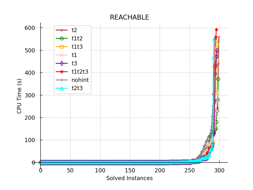
Figure 4: Cactus plot of reachable instances

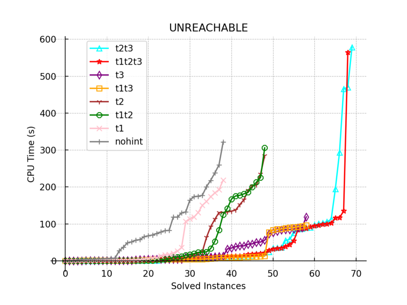
Figure 5: Cactus plot of unreachable instances

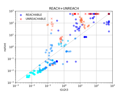
Figure 6: Scatter plot of CPU times comparing nohint and t1t2t3

We show cactus plots in Figures 5 and 5 to visually summarize our benchmark results. The graph plots how many instances can be solved in a given time-limit. The horizontal axis indicates the number of solved instances, and the vertical axis indicates CPU times in seconds for reachability checking. For unreachable instances, in Figure 5, we can observe that there is a clear gap between the top four encodings with t3 and the bottom four without it. That is, this cactus plot illustrates that our t3 hint can significantly enhance the performance of deciding unreachability.

For a more detailed analysis of this effect, a scatter plot of the comparison on CPU times between nohint and t1t2t3 is shown in Figure 6. Reachable and unreachable instances are indicated in blue and red, respectively. The darker the color of each mark, the larger the “scale” of instance. Here, the scale of instance is calculated by the product of the number of nodes in the input graph and the length of the reconfiguration sequence. The scatter plot shows that the t1t2t3 hints are able to efficiently determine the unreachability of many large instances colored by dark red in the upper right part.

Table 4: Comparison with a ZDD-based approach

benchmark family	#instances	ZDD (ddreconf)	ASP (t1t2t3)
color04	304	141	245
queen	66	60	46
sp	60	60	60
square	12	12	12
total	442	273	363

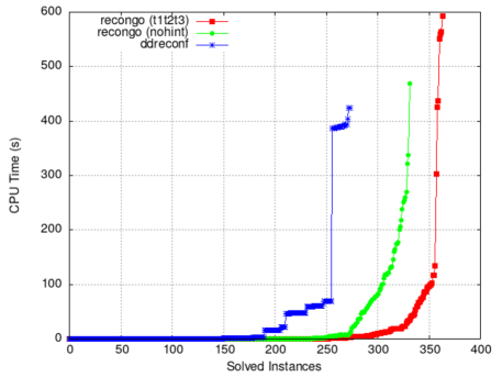
Figure 7: Cactus plot comparing ASP-based and ZDD-based approaches

Comparison with other approaches. Our comparison considers a state-of-the-art approach to CRP solving based on Zero-suppressed binary Decision Diagrams (ZDD; Ito et al. (2023)). We use the ZDD-based CRP solver ddreconf  ranked third in several metrics of the CoRe Challenge 2023. For a given DSRP instance (i.e., a DSP instance and start and goal states), ddreconf first constructs a ZDD representing all solutions of DSP. And then, it incrementally constructs ZDDs $Z^{i}$ representing all dominating sets that are reachable from the start state in exactly $i$ steps, excluding ones that are reachable in less than $i$ steps. If $Z^{i}$ includes the goal state, ddreconf returns a reconfiguration sequence. We ran ddreconf on the same environment as before.

Comparison results are shown in Table 4. The columns display in order the benchmark family, the number of instances belonging to each family, the number of solved instances for each approach. The better results of the last two columns are highlighted in bold. Overall, our declarative approach performed well compared to a ZDD-based approach. Our ASP encoding with recongo solved 363 out of 442 instances, which is 90 more than ddreconf. Our encoding with recongo showed good performance for the color04 family including many kinds of graphs, but less effective for the queen family consisting of only graphs for queens puzzles. The cactus plot in Figure 7 illustrates a clear difference in performance between ASP-based and ZDD-based approaches.

Summary and discussion. Our basic ASP encoding in Listing 4 solved 331 instances without any hint constraints. In contrast, our best encoding involving t1t2t3 hints solved 363 instances. The improvement by ASP is therefore 331 instances, and the additional 32 instances are contributed by our hint constraints. From the perspective of ZDD versus ASP in Figure 7, ddreconf and recongo(nohint) solved 273 and 331 instances, respectively. This result shows that our ASP-based method is more effective in DSRP solving than ZDD, even without the help of hint constraints. .

The most recent competition (CoRe challenge 2023) has six metrics in the single solver track. The independent set reconfiguration problems under the token jumping have been used in CoRe challenge 2023. The recongo solver won four gold and two silver medals, which is followed by two gold and four silver medals of PARIS Christen et al. (2023), and by six bronze medals of ddreconf. The gap between recongo and ddreconf at the competition is very similar to the results on DSRPs in Table 4. We used the ddreconf solver in our comparison, since, among solvers that participated in a series of CoRe challenge, only ddreconf can deal with dominating set reconfiguration. In principle, it is possible for other CRP solvers like PARIS to handle it, but significant efforts of high-level modeling and/or encoding are needed.

6 Related work

Recent advances in ASP such as multi-shot ASP solving Gebser et al. (2019) encourage researchers to tackle hard problems in combinatorial reconfiguration. The use of multi-shot ASP for combinatorial reconfiguration was first studied in Yamada et al. (2023); Yamada et al. (2024). They proposed a general approach called bounded combinatorial reconfiguration for solving combinatorial reconfiguration problems based on ASP, including algorithms, solver developments, encodings, and empirical analysis. The resulting ASP-based solver recongo is an award-winning solver of the most recent CoRe challenge 2022 and 2023.

The bounded combinatorial reconfiguration has been applied to some specific reconfiguration problems. Yamada et al. (2023); Yamada et al. (2024) developed a collection of ASP encodings for independent set reconfiguration under the token jumping rule, including basic encodings for problem solving and some hint constraints. Hirate et al. (2023) explored Hamiltonian cycle reconfiguration under the well-known k-opt rule of the traveling salesperson problem. They presented new ASP encodings for solving Hamiltonian cycle problems and extended one of them for Hamiltonian cycle reconfiguration.

This paper tackled the dominating set reconfiguration problem (DSRP). The major contribution of this paper is the development of ASP encodings and a hint constraint (named token destination) for DSRP solving under token jumping as well as token addition-removal. Particularly, our best hint constraint is shown to be highly effective in deciding unreachability. This hint is domain-specific to DSRP and is different from the ones used in the previous works Yamada et al. (2023); Yamada et al. (2024); Hirate et al. (2023). Our approach has a similarity to the previous works in the sense that both the grounding and solving tasks are delegated to the recongo solver.

There is a rapidly growing interest in the practical aspects of combinatorial reconfiguration. However, many important problems remain untouched, such as the connectivity, optimality, and diameter of the solution space. We will investigate the possibility of using ASP for those challenging problems.

7 Conclusion

We developed an approach to solve the dominating set reconfiguration problem based on Answer Set Programming (ASP). Our declarative approach relies on a high-level ASP encoding, and both the grounding and solving tasks are delegated to the ASP-based combinatorial reconfiguration solver recongo. We established the competitiveness of our declarative approach by empirically contrasting it to a more algorithmic ZDD-based approach. All source code and benchmark problems are available from the web. 

Future work includes benchmark generation for DSRP under token addition-removal, using real-data of social and sensor networks. From a broader perspective, combinatorial reconfiguration is related to automated planning, in the sense of transforming a given state to another state. It would be interesting to study the relationship between them and investigate the possibility of their synergy. For a synergy, we plan to develop a framework of cost-optimal combinatorial reconfiguration with multiple adjacency relations.

References

- Blum et al. (2005) Blum, J., Ding, M., Thaeler, A., and Cheng, X. 2005. Connected dominating set in sensor networks and manets. In Handbook of Combinatorial Optimization, D.-Z. Du and P. M. Pardalos, Eds. Springer, 329–369.
- Bonamy et al. (2021) Bonamy, M., Dorbec, P., and Ouvrard, P. 2021. Dominating sets reconfiguration under token sliding. Discrete Applied Mathematics 301, 6–18.
- Bonsma and Cereceda (2009) Bonsma, P. S. and Cereceda, L. 2009. Finding paths between graph colourings: PSPACE-completeness and superpolynomial distances. Theoretical Computer Science 410, 50, 5215–5226.
- Brewster et al. (2016) Brewster, R. C., McGuinness, S., Moore, B. R., and Noel, J. A. 2016. A dichotomy theorem for circular colouring reconfiguration. Theoretical Computer Science 639, 1–13.
- Cereceda et al. (2011) Cereceda, L., van den Heuvel, J., and Johnson, M. 2011. Finding paths between 3-colorings. Journal of Graph Theory 67, 1, 69–82.
- Christen et al. (2023) Christen, R., Eriksson, S., Katz, M., Muise, C., Petrov, A., Pommerening, F., Seipp, J., Sievers, S., and Speck, D. 2023. PARIS: planning algorithms for reconfiguring independent sets. In Proceedings of the 26th European Conference on Artificial Intelligence (ECAI 2023), K. Gal, A. Nowé, G. J. Nalepa, R. Fairstein, and R. Radulescu, Eds. Frontiers in Artificial Intelligence and Applications, vol. 372. IOS Press, 453–460.
- Denecker et al. (2009) Denecker, M., Vennekens, J., Bond, S., Gebser, M., and Truszczynski, M. 2009. The second answer set programming competition. In Proceedings of the 10th International Conference on Logic Programming and Nonmonotonic Reasoning (LPNMR 2009). LNCS, vol. 5753. Springer, 637–654.
- Gebser et al. (2019) Gebser, M., Kaminski, R., Kaufmann, B., Lindauer, M., Ostrowski, M., Romero, J., Schaub, T., Thiele, S., and Wanko, P. 2019. Potassco User Guide, Version 2.2.0 ed.
- Gebser et al. (2019) Gebser, M., Kaminski, R., Kaufmann, B., and Schaub, T. 2019. Multi-shot ASP solving with clingo. Theory and Practice of Logic Programming 19, 1, 27–82.
- Gopalan et al. (2009) Gopalan, P., Kolaitis, P. G., Maneva, E. N., and Papadimitriou, C. H. 2009. The connectivity of boolean satisfiability: Computational and structural dichotomies. SIAM Journal on Computing 38, 6, 2330–2355.
- Haas and Seyffarth (2014) Haas, R. and Seyffarth, K. 2014. The k-dominating graph. Graphs and Combinatorics 30, 3, 609–617.
- Haddadan et al. (2016) Haddadan, A., Ito, T., Mouawad, A. E., Nishimura, N., Ono, H., Suzuki, A., and Tebbal, Y. 2016. The complexity of dominating set reconfiguration. Theoretical Computer Science 651, 37–49.
- Hearn and Demaine (2005) Hearn, R. A. and Demaine, E. D. 2005. Pspace-completeness of sliding-block puzzles and other problems through the nondeterministic constraint logic model of computation. Theoretical Computer Science 343, 1-2, 72–96.
- Hearn and Demaine (2009) Hearn, R. A. and Demaine, E. D. 2009. Games, puzzles and computation. A K Peters.
- Hirate et al. (2023) Hirate, T., Banbara, M., Inoue, K., Lu, X., Nabeshima, H., Schaub, T., Soh, T., and Tamura, N. 2023. Hamiltonian cycle reconfiguration with answer set programming. In Proceedings of the 18th Edition of the European Conference on Logics in Artificial Intelligence (JELIA 2023), S. A. Gaggl, M. V. Martinez, and M. Ortiz, Eds. Lecture Notes in Computer Science, vol. 14281. Springer, 262–277.
- Huynh (2020) Huynh, M. K. 2020. Solving dominating set using answer set programming. M.S. thesis, Heinrich Heine Universität düsseldorf.
- Inoue et al. (2014) Inoue, T., Takano, K., Watanabe, T., Kawahara, J., Yoshinaka, R., Kishimoto, A., Tsuda, K., Minato, S., and Hayashi, Y. 2014. Distribution loss minimization with guaranteed error bound. IEEE Transactions Smart Grid 5, 1, 102–111.
- Ito et al. (2011) Ito, T., Demaine, E. D., Harvey, N. J. A., Papadimitriou, C. H., Sideri, M., Uehara, R., and Uno, Y. 2011. On the complexity of reconfiguration problems. Theoretical Computer Science 412, 12-14, 1054–1065.
- Ito et al. (2023) Ito, T., Kawahara, J., Nakahata, Y., Soh, T., Suzuki, A., Teruyama, J., and Toda, T. 2023. ZDD-based algorithmic framework for solving shortest reconfiguration problems. In Proceedings of the 20th International Conference on the Integration of Constraint Programming, Artificial Intelligence, and Operations Research (CPAIOR 2023), A. A. Ciré, Ed. Lecture Notes in Computer Science, vol. 13884. Springer, 167–183.
- Ito et al. (2015) Ito, T., Ono, H., and Otachi, Y. 2015. Reconfiguration of cliques in a graph. In Proceedings of the 12th Annual Conference on Theory and Applications of Models of Computation (TAMC 2015), R. Jain, S. Jain, and F. Stephan, Eds. Lecture Notes in Computer Science, vol. 9076. Springer, 212–223.
- Kaminski et al. (2012) Kaminski, M., Medvedev, P., and Milanic, M. 2012. Complexity of independent set reconfigurability problems. Theoretical Computer Science 439, 9–15.
- Knuth (2011) Knuth, D. 2011. The art of computer programming Vol.4A, Combinatorial algorithms, Part 1. Addison-Wesley.
- Lifschitz (2019) Lifschitz, V. 2019. Answer Set Programming. Springer-Verlag.
- Mohar and Salas (2009) Mohar, B. and Salas, J. 2009. A new kempe invariant and the (non)-ergodicity of the wang–swendsen–kotecký algorithm. Journal of Physics A: Mathematical and Theoretical 42, 22 (may), 225204.
- Mouawad et al. (2017) Mouawad, A. E., Nishimura, N., Pathak, V., and Raman, V. 2017. Shortest reconfiguration paths in the solution space of boolean formulas. SIAM Journal on Discrete Mathematics 31, 3, 2185–2200.
- Nishimura (2018) Nishimura, N. 2018. Introduction to reconfiguration. Algorithms 11, 4, 52.
- Soh et al. (2024) Soh, T., Tanjo, T., Okamoto, Y., and Ito, T. 2024. CoRe challenge 2022/2023: Empirical evaluations for independent set reconfiguration problems (extended abstract). In Proceedings of the Seventeenth International Symposium on Combinatorial Search (SOCS 2024), A. Felner and J. Li, Eds. AAAI Press, 285–286.
- Suzuki et al. (2016) Suzuki, A., Mouawad, A. E., and Nishimura, N. 2016. Reconfiguration of dominating sets. Journal of Combinatorial Optimization 32, 4, 1182–1195.
- Takaoka (2018) Takaoka, A. 2018. Complexity of hamiltonian cycle reconfiguration. Algorithms 11, 9, 140.
- Toda et al. (2023) Toda, T., TakehiroIto, Kawahara, J., Soh, T., Suzuki, A., and Teruyama, J. 2023. Solving reconfiguration problems of first-order expressible properties of graph vertices with boolean satisfiability. In Proceedings of the IEEE 35th International Conference on Tools with Artificial Intelligence (ICTAI 2023). 294–302.
- van den Heuvel (2013) van den Heuvel, J. 2013. The complexity of change. In Surveys in Combinatorics 2013, S. R. Blackburn, S. Gerke, and M. Wildon, Eds. London Mathematical Society Lecture Note Series, vol. 409. Cambridge University Press, 127–160.
- Yamada et al. (2023) Yamada, Y., Banbara, M., Inoue, K., and Schaub, T. 2023. Recongo: Bounded combinatorial reconfiguration with answer set programming. In Proceedings of the 18th Edition of the European Conference on Logics in Artificial Intelligence (JELIA 2023), S. A. Gaggl, M. V. Martinez, and M. Ortiz, Eds. Lecture Notes in Computer Science, vol. 14281. Springer, 278–286.
- Yamada et al. (2024) Yamada, Y., Banbara, M., Inoue, K., Schaub, T., and Uehara, R. 2024. Combinatorial reconfiguration with answer set programming: Algorithms, encodings, and empirical analysis. In Proceedings of the 18th International Conference and Workshops on Algorithms and Computation (WALCOM 2024), R. Uehara, K. Yamanaka, and H. Yen, Eds. Lecture Notes in Computer Science, vol. 14549. Springer, 242–256.