Work and Activation in a Nematic Polymer Network Ribbon
Abstract
We study spontaneous deformations of a ribbon made of nematic polymer networks and activated under the action of a mechanical load. We show that when such ribbons are activated appropriately, the deformations produced can pull back and perform work against the externally applied load. We perform two numerical experiments to demonstrate this effect: (1) the pulling experiment, where the ribbon is pulled longitudinally by a point force, and (2) the bending experiment, where the ribbon is bent out of plane by a terminally applied point force. We quantify the capacity of the ribbon to work against external loads, and compute its dependence on both the ribbon thickness and the imprinted nematic texture (that is, the distribution of the nematic directors across the ribbon’s length). Finally, we compute the efficiency of the activation process. Building on the outcomes of our numerical explorations, we formulate two educated conjectures on how the activation efficiency can in general be improved by acting on both the applied load and the imprinted nematic texture.
I Introduction
Liquid crystal elastomers (LCEs) are rubber-like materials impregnated with nematogenic molecules, which as parts of the polymeric network composing the material have the potential of affecting the network’s shape in consequence of the long-range order that characterizes their molecular organization.
A thorough introduction to these fascinating materials and the theories that describe their behaviour is the already classic book [1]; several reviews are also available [2, 3, 4, 5, 6, 7, 8]; a recent addition to these is [9], which in its witty style and historical perspective makes a very enjoyable reading.
General continuum theories of these materials are available: we only cite [10, 11, 12, 13], being fully aware that this is an incomplete list. Applications are likewise manifold; a special issue [14] collects a few.
As acutely remarked in [9], LCEs are indeed expected to find much more uses than they presently do: they should only be “brought out of research labs.” This is because LCEs are more versatile materials than classic shape memory polymers, which have already many industrial applications [15, 16]. Unlike the latter, which can change shape only once, LCEs can switch reversibly between two programmable shapes under the action of an appropriate external stimulus.
We may say that conventional rubber is a liquid impeded to flow by the entanglement of cross-links that confers to the material a solid-like response. With a parallel metaphor, we may also say that a LCE is liquid crystal suffering a similar fate. The additional degrees of freedom that arise in LCEs compared to conventional elastomers are described by the nematic director field ,111The symbol is most often used to denote the nematic director; here we deviate from tradition to avoid clash with the typical notation for the internal force in a framed curve, which will be introduced in the following section. which represents the orientation of liquid-crystalline molecules in their condensed phase, and by a scalar order parameter , which represents the degree of orientational order present locally. These extra fields are responsible for the fascinating mechanical behaviour of LCEs, mostly stemming from their coupling with conventional kinematic measures.
There are several classes of LCEs; we shall be confined here to nematic LCEs (actually, to a subclass of these), in which molecules tend to orient alike, but their positions in space are disordered. As remarked in [4], nematic LCEs are known under a variety of names, not all synonyms. Nominalistic nuances apart, what effectively makes the difference between them (and should be reflected in their appellation) is the extent of cross-linking: the higher this is, the stiffer the material becomes and more is the nematic director linked to the polymer network motion.
When is completely ensalved to the macroscopic deformation, which is the case for extreme cross-linking, LCEs are called nematic polymer networks (NPNs).222They are also called nematic glasses in [17] and lately also glassy liquid crystal networks [9], a newly added name to the already abundant taxonomy of LCEs.
In this paper, we shall only be concerned with NPNs. Several mechanisms are capable of inducing a change in the degree of order among the nematogenic constituents of the polymer chains in NPNs. They range from heat exchanges modifying the temperature to illumination with frequencies triggering the morphing of dispersed dyes affecting the ordering of the nematic molecules. Light can be an actuator as good as heat, with the advantage of being able to act contactlessly.333To describe the interplay between nematic ordering and photon absorption, models with a statistical mechanics twist have also been proposed [12, 18, 19, 20, 21, 22, 23] (see also [24] for a recent review).
In this paper, following the theory put forward in [25], we shall remain agnostic about the specific mechanism at play to change the ordering in the nematic molecular organization. We shall assume that a uniform scalar order parameter characterizes the nematic order in the reference configuration and another scalar order parameter (still uniform) characterizes the nematic order in the present configuration. Letting amounts to activating the material. If , nematic molecules become more aligned along the director ; if , they become less oriented along . We shall also assume that the cross-linking of the material takes place in the reference configuration, so that and are prescribed there. By changing into , the system is brought out of equilibrium and a spontaneous deformation ensues that conveys into in a material fashion, so that
| (1) |
where is the deformation gradient. is here the only activation parameter.
Our setting will not be three-dimensional. We shall adopt a theory for thin NPN sheets that was obtained in [26] by dimension reduction of the celebrated trace-formula for the elastic free-energy density (per unit volume), which has a long history [27, 28, 29, 30] (see also Chap. 3 of [1]).
The theory presented in [26], building upon an extension of the classical Kirchhoff-Love hypothesis of plate theory [31], arrives at an elastic free-energy density (per unit area) for a thin NPN sheet featuring two separate contents, a stretching content scaling like the sheet’s thickness , and a bending content scaling like . This theory will be adopted here in the limit where the NPN sheet under consideration can be regarded as a narrow ribbon, as in the previous study [25]. Moreover, as in [32], special attention will be devoted to the role played by in driving stretching and bending deformation modes. The major novelty of the present study lies perhaps in the presence of external mechanical loads that can interfere with the spontaneous deformation prompted by activation.
A NPN ribbon will be described as a framed material curve, albeit with a rather unorthodoxal energy. In Sect. II, we find it convenient to rephrase afresh in our context the Lagrangian theory of framed material curves, which will then be used in Sect. IV to obtain the system of equilibrium equations for a NPN ribbon, after having recalled in Sect. III the energetics of the parent mechanical theory for nematic elastomers in three space dimensions, to make our development self-contained. The governing equations turn out to be so intricate not to be amenable to an analytic treatment; even numerics must be adapted in Sect. V to tackle the hybrid character (both differential and finite) of these equations. Section VI is devoted to two numerical experiments where a cantilever ribbon is pulled or bent prior to activation. Both qualitative and quantitative aspects of the calculated solutions are presented, some being unexpected. In Sect. II, much in the spirit of [33], we introduce and compute a measure of actuation efficiency for both experiments, paying special attention to the factors, either geometric or mechanical, that can enhance it. Finally, in Sect. VIII, we collect the conclusions of this study.
II Lagrangian theory of framed material curves
By a framed material curve we mean a smooth curve endowed with an orthonormal frame of directors , where is any scalar parameter whose values identify material points on . We restrict our interest to curves where is constrained to lie along the tangent , with prime being derivation with respect to . We will refer to such a curve as an adapted framed curve, which is completely determined by the set (see Chapt. VIII of [34]). The kinematics of an adapted framed curve are described by the following two relations,
| (2) |
The first constraint in (2) ensures that is parallel to the tangent, with , while the second relation ensures the orthonormality of the director frame as it evolves along the paramater . Vector in (2)2 is the Darboux vector associated with the frame .
Consider the following action functional defined on an adapted framed curve,
| (3) |
Here, the Lagrangian is the energy density function444We consider to depend on the first derivatives of and only, since it fits the description of our functional of interest. However, the method outlined below can be applied to functionals containing higher order derivatives. associated with the framed curve, , , and , , are a number (indexed in ) of additional ancillary functions, whose role will be highlighted in the following. The second integral enforces constraint (2)1 in a pointwise manner through a Lagrange multiplier function . The third integral accounts for the potential associated with any point force possibly acting at one of the two terminal ends. Without any loss of generality, we assume that this point force is acting at . We shall consider as a surrogate for time; in line with this, we shall often refer to equations involving derivatives in as evolution equations.
Our objective is to minimize the action functional in (3) in the set of all admissible configurations consistent with the boundary conditions at hand. While the procedure we outline does not depend on the nature of the prescribed boundary conditions, we will assume the following boundary conditions which arise in the specific problems we wish to study below,
| (4) |
where is an assigned vector and is a given Cartesian frame.
Consider the following variations in the configuration of an adapted framed curve,
| (5) |
where is subject to the condition due to (4), whereas and are arbitrary. The variations must be such that the frame is also orthonormal. This constrains the variations to be of the form,
| (6) |
where is an abitrary vector-valued function. The variation will further induce a variation in the Darboux vector,
| (7) |
To express in terms of , with the aid of (6) and (2)2 we transform the equation into the identity
| (8) |
Since is a basis, we conclude from (8) that
| (9) |
Using (9) and (6), the variations can be written as
| (10) |
Next, the variation of the action functional (3), induced by variations (5), can be computed in the standard way as,
| (11) |
where sum over repeated indices is understood. On integrating by parts, and using (6) and (10), can be written as,
| (12) |
To require that , we invoke the arbitrariness of the variations in the bulk and we write down the governing equations in the following transparent form,
| (13a) | ||||
| (13b) | ||||
| (13c) | ||||
| (13d) | ||||
where,
| (14) |
We have used in writing (13b). As can be clearly seen, equations (13a) and (13b) are formally the Kirchhoff rod equations of force and moment balance, accompanied by (what can be interpreted as) constitutive relations (14) for the internal moment. When the energy density is independent of , the constitutive relations (14) reduce to the standard constitutive relation for a hyperelastic rod (see again Chap. VIII of [34]). Also, one can interpret (13d) as a constitutive relation for . Equations (13a) and (13b) are the vector representations of equations (15) and (16) of Hornung’s article [35], and equations (32) and (33) of Starostin’s article [36]. Equation (14) corresponds to equation (14) of [35], and equation (34) of [36].
To obtain the boundary conditions, we note that (4) and (6) imply that , , using which we conclude from (12) that
| (15a) | ||||
| (15b) | ||||
| (15c) | ||||
| (15d) | ||||
Equations (13)-(15) form the basis of our general Lagrangian theory for framed material curves, where time is replaced by arc-length. In Sect. IV, we shall apply it to the deformation of an activable soft material, after a brief digression about the energetics of nematic elastomers.
III Energetics of nematic elastomers
Our theory is based on the trace formula for the elastic free-energy density (per unit volume of the reference configuration) proposed in [37] for nematic elastomers,
| (16) |
where is the number of polymer strands per unit volume, is the temperature in the reference configuration, is the deformation gradient, and and are the step-length tensors in the present and reference configurations, respectively.
The latter tensors reflect the organization of nematogenic molecules within the polymer network. Following [38, 39], we represent them as
| (17) |
where is the identity tensor (in three-dimensional space), and are the nematic directors in the reference and present configurations, and and the corresponding scalar order parameters. These parameters are related to the nematic scalar order parameters and of the classical Maier-Saupe theory through the equations,
| (18) |
while the amplitudes and are given by
| (19) |
where is the length of the rod representing a single monomer in the classical statistical mechanics model that describes a polymer strand as a chain of freely jointed equal rods. It follows from (18) and (19) that
| (20) |
The nematic scalar order parameter is defined as
| (21) |
where is the second Legendre polynomial, is the unit vector designating the orientation of a single monomer, and the brackets denote ensemble average. The same formula applies to , with replaced by . It is an easy consequence of (21) that ranges in the interval , the upper end designating the (ideal) state of perfect orientation of all molecules along and lower end representing the state of isotropic orientation in the plane orthogonal to . Correspondingly, by (18), . Here both and will be taken as positive.
Changing the degree of order (measured by either or ) costs energy, which is accounted for by the condensation free-energy density (per unit volume) arrived at in the mean-field theory of Maier and Saupe [40, 41], as described, for example, in Sect. 1.3 of [42],
| (22) |
where is the number density of nematogenic molecules and
| (23) |
In (23), is the Maier-Saupe molecular interaction energy (scaled to ) and is the Dawson integral, defined as
| (24) |
Moreover, is related to as in (20).
The absolute minimizer of depends on ; for , it is equal to , as delivered by (20) in terms of the scalar order parameters imprinted in the reference configuration at the time of cross-linking.
Here, for simplicity, we shall consider as a control parameter, ascribing to external causes the change in the value of away from which is responsible for shifting the absolute minimizer of the potential from to .
Since also depends on , a more orthodox approach would be to use as a control parameter and let the total free-energy density decide the equilibrium value of in competition with the elastic deformation. Our approach is however justified by the assumption that the elastic deformation is a much slower response compared to the activation processes that we envision, which will be taken as virtually instantaneous. Under this assumption, were we only interested in the mechanical response of the system, we could safely disregard all energies that depend only on , as done for example in [25, 32]. Here, for use in Sect. VII, we keep all these energies as well, as we are also interested in the estimate of the activation energy and the efficiency of the mechanical yield.
In summary, we write the total free-energy density as
| (25) |
where is the right Cauchy-Green tensor and use has also been made of the kinematic constraint (1) (see also [25, 32]). In (III), is the function in (20) and is such that is minimized by . The parameter
| (26) |
describes the degree of cross-linking in the material: the larger , the stronger the cross-linking. Following [20], for strongly cross-linked polymers, such as NPNs, we shall choose .
IV A nematic polymer network ribbon
Here we consider a ribbon comprised of nematic polymer networks. We assume that it is sufficiently narrow to be treated within our theory for framed curves. The reference configuration, a rectangle of width and length , is depicted in Fig. 1.

The (scaled) elastic free-energy density (per unit normalized length) of a thin NPN ribbon was derived in [32] from a dimension reduction of in (16) [see, in particular, their equations (43) and (44)]. By applying the same method, here, starting from (III) we arrive at the following expression,
| (27) |
Here and represent the scalar order parameter in the reference and present configurations, respectively, and and describe the orientation relative to the ribbon’s centerline of the nematic director in the reference and present configurations, respectively. In (27) and in the following, energies are rescaled to the characteristic energy555The scaling factor of the energy differs slightly from the one, , employed in [25]; the two are related by the equation which is recorded for ease of future reference.
| (28) |
Moreover, all lengths are scaled to , including , which represents the ribbon’s thickness. Thus, in particular, will range in and , as dictated by the small-thickness assumption adopted in [26, 25]. As customary in plate theory, bending and stretching energies are weighted one relative to the other as versus ; all energies of order or higher are neglected.
We regard as a control parameter that says whether the nematic order has been enhanced () or depressed () by external agents relative to the order imprinted in the reference configuration. Correspondingly, the angle designates the orientation of the nematic director imprinted in the reference configuration (see Fig. 1); it varies with the arc-length along the centerline of the ribbon and affects the way a given change from to induced by activation affects the elastic response of the ribbon.
In the present setting of a rectangular ribbon with width and length depicted in Fig. 1,
| (29) |
while the position vector is represented by the mapping
| (30) |
The angle designates the orientation of the nematic director in the present configuration,
| (31) |
In a NPN, an area-preserving deformation , which is defined on a surface and takes values in three-dimensional space [26], conveys the nematic director as a material line, as prescribed by (1). This, combined with the kinematic analysis in [25] and [32], leads us to conclude that is described by the mapping
| (32) |
where
| (33) |
It thus remains fully justified that the elastic energy density in (27), which describes a blend of stretching and bending energy contents, depends on the kinematic variables and has as parameters.
As shown in [32] [see, in particular, their equation (46)], the incompressibility constraint is written as,
| (34) |
In (27) and (34), we perform a change of variables replacing with . Consequently, is replaced by . The resulting functional in (3), augmented with the transformed representation of (34), is represented by the Lagrangian
| (35) |
where is a pointwise Lagrange multiplier function corresponding to the incompressibility constraint. In (35), plays the role of a single ancillary function of the many ’s featuring in the general form of in (3).
Similarly, the constitutive equations (14) are changed as follows by the intervention of the new variable ,
| (36a) | ||||
| (36b) | ||||
| (36c) | ||||
IV.1 Equilibrium equations
The configuration space of an NPN ribbon, modulo translations and rigid rotations, is spanned by the functions where and , with , are the director components of the internal force and internal moment . Their evolution in is governed by (13a) and (13b) written in the director components, and subsequently transformed by introducing ,
| (37a) | ||||
| (37b) | ||||
| (37c) | ||||
| (37d) | ||||
| (37e) | ||||
| (37f) | ||||
Next we write down the constitutive equations for explicitly using (35) and (36). We note that the square bracketed term in (36a) can be eliminated using (36c). From this, along with the relations and , we obtain
| (38) |
Using (35) in (38), we arrive at the following explicit expression for ,
| (39) |
Similarly, by some calculations and use of (35) and (37e), equations (36b) and (36c) can be written as,
| (40) |
| (41) |
the latter of which makes also use of the former. Furthermore, the equilibrium equation corresponding to can be obtained from (13c) as,
| (42) |
which is simply the inextensibility constraint rearranged. Finally, using (13d) and (35), the equilibrium equation for the stretch can be written as,
| (43) |
IV.2 Kinematic equations
The centerline of the ribbon can be obtained by integrating relation (2)1. To that end we parametrise the director frame attached to the centerline using the quaternion parameter , where , subject to the constraint of unit norm (see, for example, [43, 44]).666Often the four rotation parameters are called the Euler-Rodrigues parameters in the literature. However, as noted in [45], this attribution is disreputable. The Cartesian components of the directors in a fixed lab frame can then be represented as
| (44) |
Using the above in (2)2, the evolution equations of s can be obtained as,
| (45) |
The Cartesian components of the centerline in a fixed lab frame, namely can then be obtained by integrating the following equations, which follow from (44)3 and (2)1,
| (46a) | ||||
| (46b) | ||||
| (46c) | ||||
IV.3 The full differential-algebraic system
With the parameterisation of the directors , the system of equations describing a thin NPN ribbon comprise 14 first order differential equations, and 2 algebraic equations. The differential equations are the force and moment balance equations (37), the incompressibility constraint (42), and the kinematic equations (45) and (46a), whereas the algebraic equations are (41) and (43). For brevity of notation, we represent our system as,
| (47a) | ||||
| (47b) | ||||
where are the differential functions, whereas are the algebraic variables. The vectors and are respectively the right-hand side of equations (37), (42), (46a), (45), and (41) and (43).
The system requires a total of 14 boundary conditions to be complete. We postpone the specification of these conditions until Sect. VI.
The differential-algebraic system obtained thus far is of index 2 according to the definition in [46], which means that the algebraic equations can be differentiated twice to obtain a set of ODE’s for the algebraic functions . Our attempt to obtain such a system led us to equations which contained expressions that were intractable and unmanageable. To avoid such difficulties, we chose to discretize directly the algebraic equations along with the differential ones using the method of orthogonal collocation on finite elements, the details of which are discussed in the next section.
V Numerical discretization
We follow the lecture notes of Doedel [47] to discretize our system (47) using orthogonal collocation. While Doedel’s notes focus on system of ordinary differential equations only, we modify his approach to obtain a discretization for the accompanying algebraic equations as well.
We discretise the normalized domain into finite elements of equal size such that , and denote and define the th element as , where . Our objective is to find vectors of polynomials and , where is the space of vector piecewise polynomials such that the following collocation equations,
| (48) |
are satisfied with obeying the accompanying boundary conditions. The collocation points in each sub-interval are the scaled roots of the th degree element of a system of orthogonal polynomials (Gauss points).
In each sub-interval , the vector of polynomials are approximated as
| (49) |
where , with and , are the Lagrange polynomials defined as,
| (50) |
With this choice, we have
| (51) |
where and are the solutions of the continuous problem. Furthermore, we enforce the continuity of the polynomials across elements. No such condition is imposed on the ’s approximating the algebraic functions.
The number of differential functions in our system is and the number of algebraic functions is . Since a polynomial of degree is determined by parameters, the total number of degrees of freedom of all the polynomials approximating our system is . This is equal to the number of collocation equations (48) plus the number of continuity conditions for the differential functions plus , the number of boundary conditions on the differential variables. Thus, our system is complete.
The resulting discretised algebraic equations are solved by using a pseudo-arclength continuation scheme [48].
VI A cantilever ribbon
We employ the apparatus developed so far to compute configurations of a rectangular ribbon of length and thickness under pure mechanical stretching and bending, and subsequent activation. Our end objective is to compute estimates of the work that can be recovered from a mechanically deformed ribbon by activating it.


We consider a ribbon for which the translational and rotational degrees of freedom at are constrained, and a dead load applied at the other end. The boundary conditions to be imposed on system (47a) are given by,
| (52a) | ||||
| (52b) | ||||
| (52c) | ||||
| (52d) | ||||
| (52e) | ||||
| (52f) | ||||
| (52g) | ||||
| (52h) | ||||
| (52i) | ||||
| (52j) | ||||
| (52k) | ||||
| (52l) | ||||
| (52m) | ||||
| (52n) | ||||
The distribution of the nematic directors across the length are assumed such that the angle they make with is given by
| (53) |
where is an integer. We will restrict our analysis to reference configurations with and .
For each distribution of the nematic directors, we conduct two numerical experiments, namely the pulling experiment and the bending experiment, the details of which are described in the following.
VI.1 The pulling experiment
We consider an initially straight ribbon fixed at so that the director frame coincides with the Cartesian basis , whose origin is placed at . The ribbon is mechanically stretched by a force applied at , and gradually increased from to , where is an elastic modulus of the ribbon selected so that , which by (28) amounts to set
| (54) |
The order parameter is held constant at during this process.777This specific value of has been selected so as to correspond via (20) to a Maier-Saupe order parameter , which minimizes for ; in explicit physical terms, this amounts to take the temperature , where is the temperature of the nematic-to-isotropic transition of the nematogenic molecules (also known as the clearing temperature). Subsequently, we activate the ribbon by varying quasi-statically the order parameter in the interval , while holding the load constant.888In the variable , the interval for becomes the interval , whose end-points are the absolute minimizers of for any and , respectively. This is the general setting of the pioneering experiments reported in [49] (see also [1, p. 69]).
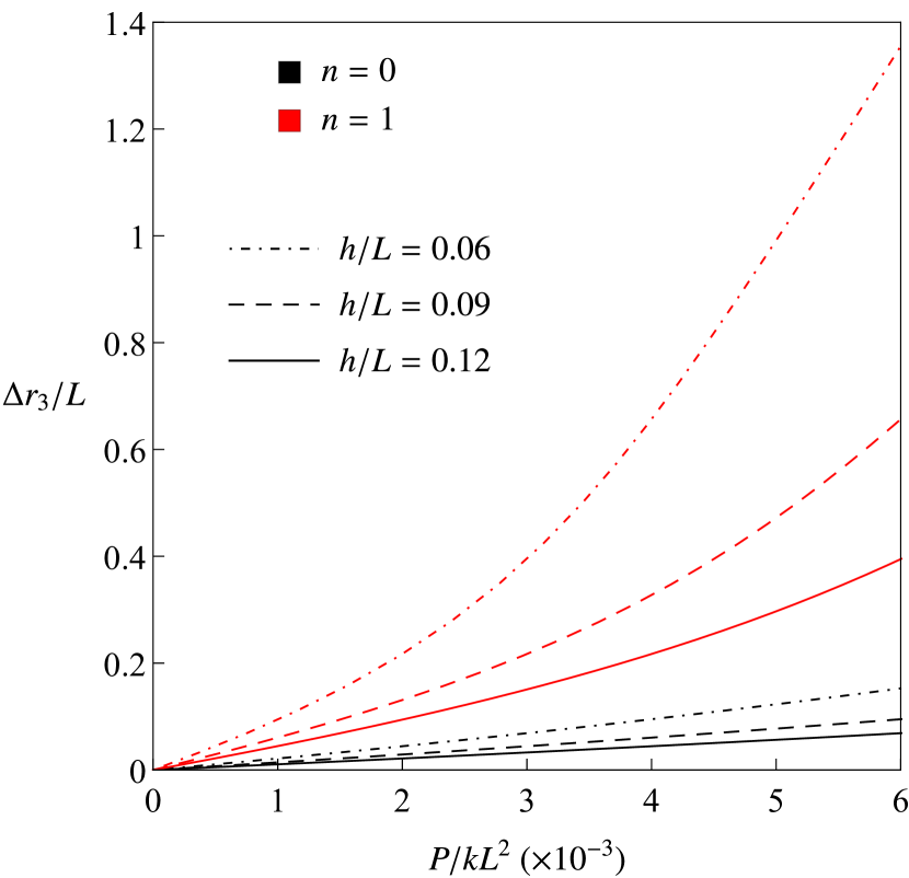
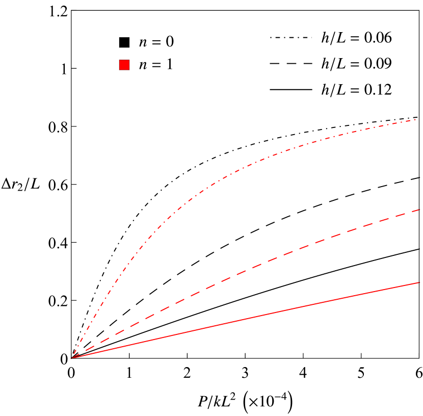
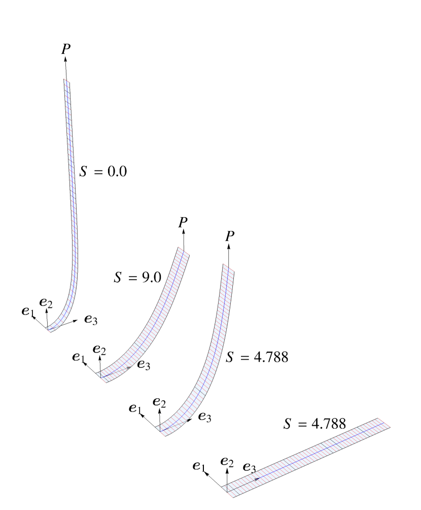
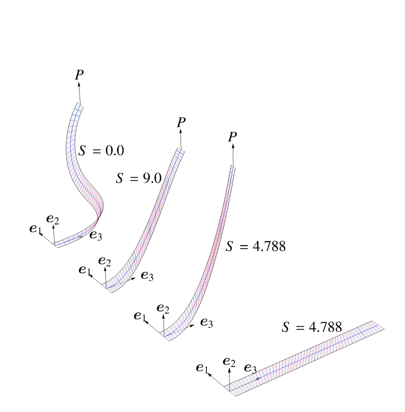
Fig. 3(a) shows the plot of the net normalized tip displacement of the ribbon () against the normalized applied force for distributions of the nematic director field corresponding to and , and different values of the normalized thickness . Since a higher thickness leads to an effectively higher axial stiffness of the ribbon, thicker ribbons undergo smaller tip displacements as compared to thinner ribbons for both and . For a given load, the net displacement of the tip remains consistently higher for as compared to , indicating that a varied distribution of the nematic directors along the length reduces the axial stiffness of the ribbon. It is worth pointing out that since the case possesses symmetry about the plane spanned by , the centerline remains straight upon deformation (see Fig. 3(c)). This symmetry is broken for the case , resulting in a deformation of the centerline in the plane upon pulling (Fig. 3(d)). We also observe that the reduction in the axial stiffness for as compared to becomes more pronounced as the load increases.
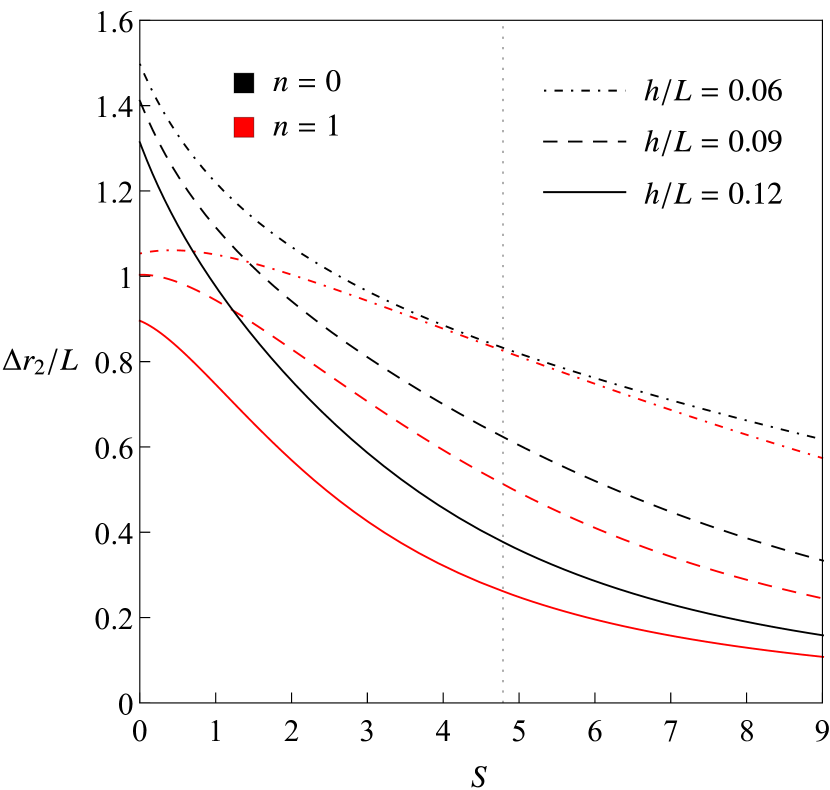
Next we activate the deformed ribbon, with applied to it, from its base state by varying from to and to . The change in the tip displacement as a function of is shown in Fig. 3(b). Here we observe a qualitative difference between the response of the ribbon for and . For , where the nematic directors are aligned orthogonally to the centerline in the reference configuration, the values of lead to a retraction of the ribbon tip in the direction opposite to the applied force. For , we observe the opposite behavior, i.e., the ribbon further elongates under the same load upon activation. This observation can be understood in light of the fact that an increase in over means an increase in the nematic order, which is accompanied by a dilation of the fibers along the nematic directors. Since the deformation is assumed to be area preserving, this leads to the shortening of the fibers orthogonal to the nematic directors, which in this case happens to be along the centerline.
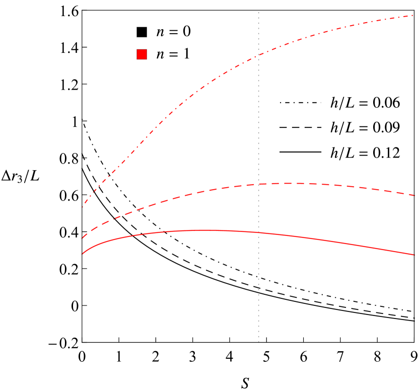
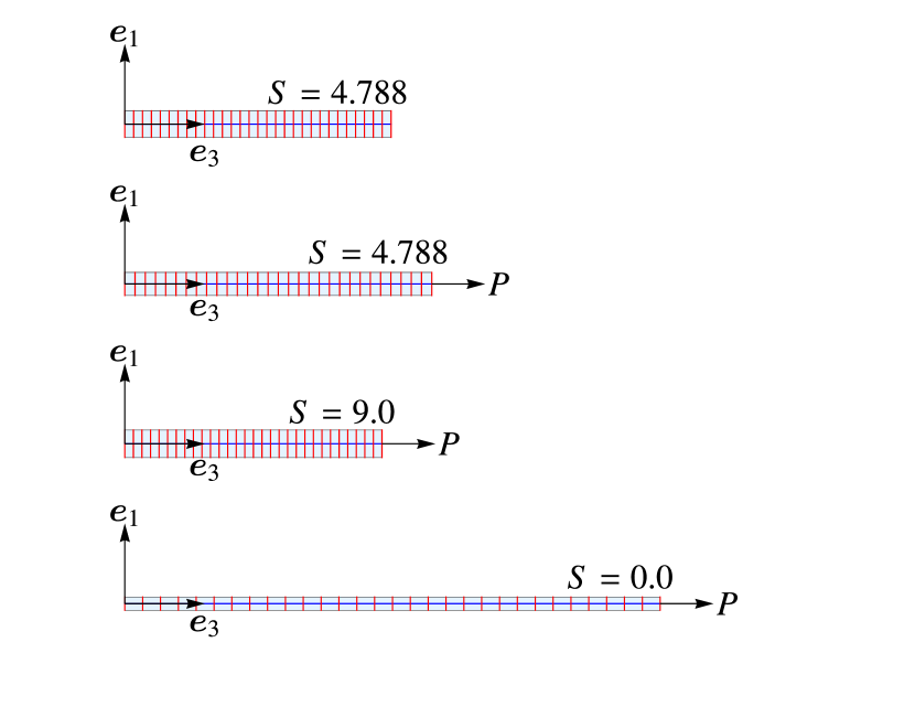
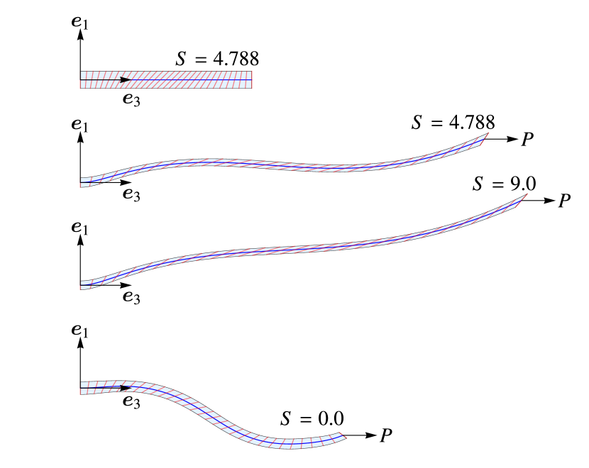
For , the behavior of the ribbon is qualitatively different from the case with . The tip of the ribbon consistently retracts against the applied load for for all the three thicknesses studied. For , whether the tip displaces along or against the load depends on the thickness of the ribbon. We observe that for , the tip displaces along the load for , whereas for and , there is a net retraction of the tip against the load. We believe that this behavior is a result of the complex interplay between the dilation/contraction of the fibers, and the shear deformation that they undergo due to the variation of the nematic director field along the length of the ribbon. Figs. 3(c) and 3(d) show various configurations of the ribbon corresponding to mechanical stretching and subsequent activation for and respectively.
VI.2 The bending experiment
Next we explore the behavior of the NPN ribbon to bending out of plane. We apply a transverse point load at , and vary its magnitude from to , while the other end remains fixed as in the pulling experiment. The order parameter is held constant at during this process.
The normalized component of the transverse displacement of the tip is plotted against the normalized load in Fig. 4(a). Contrary to the pulling experiment, we observe that the transverse displacement for the case are consistently lower than for for all thicknesses. This indicates that the anisotropy in this case produces an increase in the effective bending stiffness of the ribbon. It is also worth noting that for the ribbon strictly bends in the plane, whereas for the ribbon also twists in addition to bending (see Figs. 4(c) and 4(d)).
The deformed ribbon with a transverse tip load of is then activated by varying the order parameter from its base state of in the range . Fig. 4(b) shows the variation of the normalized tip displacement as a function of the order parameter . As opposed to the pulling experiment, the response of the ribbon to activation remains qualitatively the same for and . In both cases, the ribbon retracts for values of , whereas it deflects further for .
VII Activation efficiency
We showed in the previous section that a terminally loaded NPN ribbon can pull back on axially and transversely applied terminal point loads, if activated the right way. The activation of an NPN ribbon is achieved by driving the scalar order parameter away from its value in the reference configuration to a target value chosen so as to recover mechanical work. For the pulling experiment, the chosen target values of for and are and , respectively. For the bending experiment, the chosen target value for is for both nematic director arrangements. Such changes in the order parameter requires energy exchange between the ribbon and its environment in form of heat or light. While our theory is agnostic to the mode of energy exchange, we assume, for definiteness, that the activation is brought about by an exchange of heat. We now compute the amount of heat required to drive from to a target value . We quantify this capacity of an NPN ribbon by defining the activation efficiency as,
| (55) |
where is the mechanical yield of activation, that is, the work done by the ribbon against the point force during activation, and is the amount of heat injected into the ribbon to activate it. The mechanical yield of activation is evaluated as,
| (56) |
where , and are the positions of the free end of the ribbon centerline in the pulled, and fully activated configurations, respectively. The work is computed only for those situations where the activation leads the tip of the ribbon to displace against the applied load, and is therefore expected to be negative. For instance, in the pulling experiment, in (56) is computed for going from to for , whereas for it is computed for going from to . For the bending experiment, is computed for going from to for both and .
We compute for a given activation process from the following statement of balance of energy,
| (57) |
where and are the total energies of the ribbon (obtained by integrating (35) over the centerline) in the activated state and the purely mechanically pulled/bent state respectively.
We present the efficiency defined in (55) for both the pulling and the bending experiments against the (scaled) thickness of the ribbon in Figs. 5(a) and 5(b), respectively. In addition, we note the change in efficiency in response to two values of the applied loads and for both pulling and bending experiments.
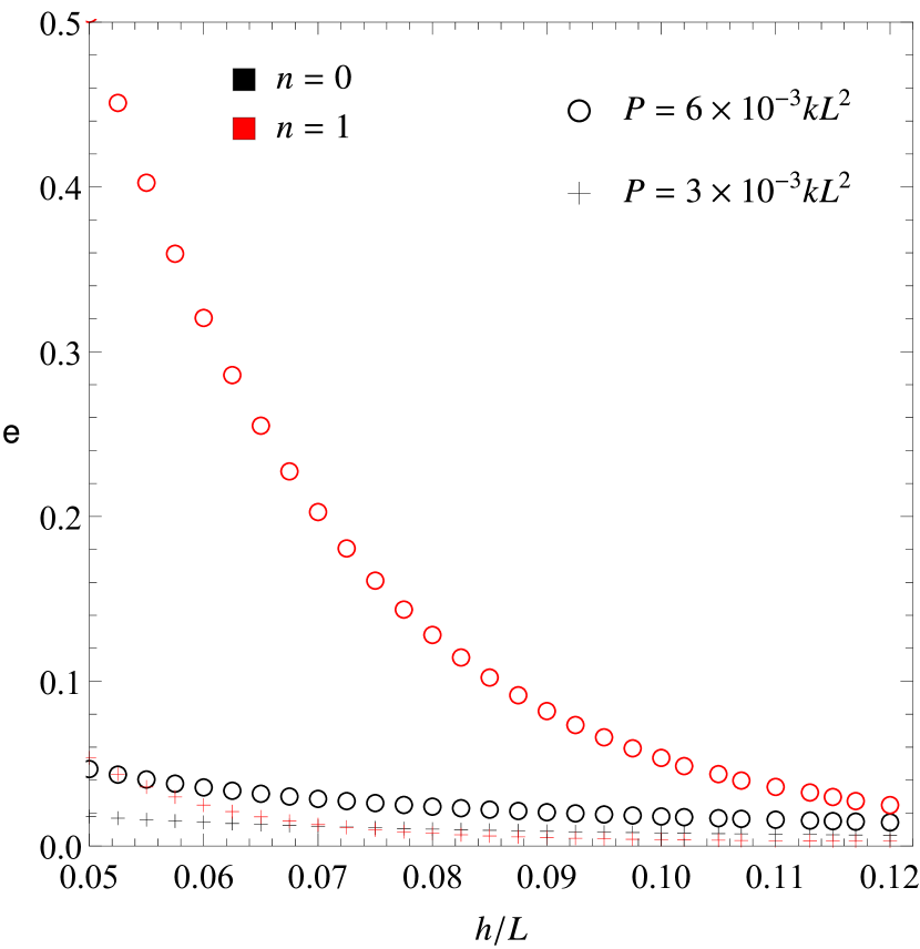
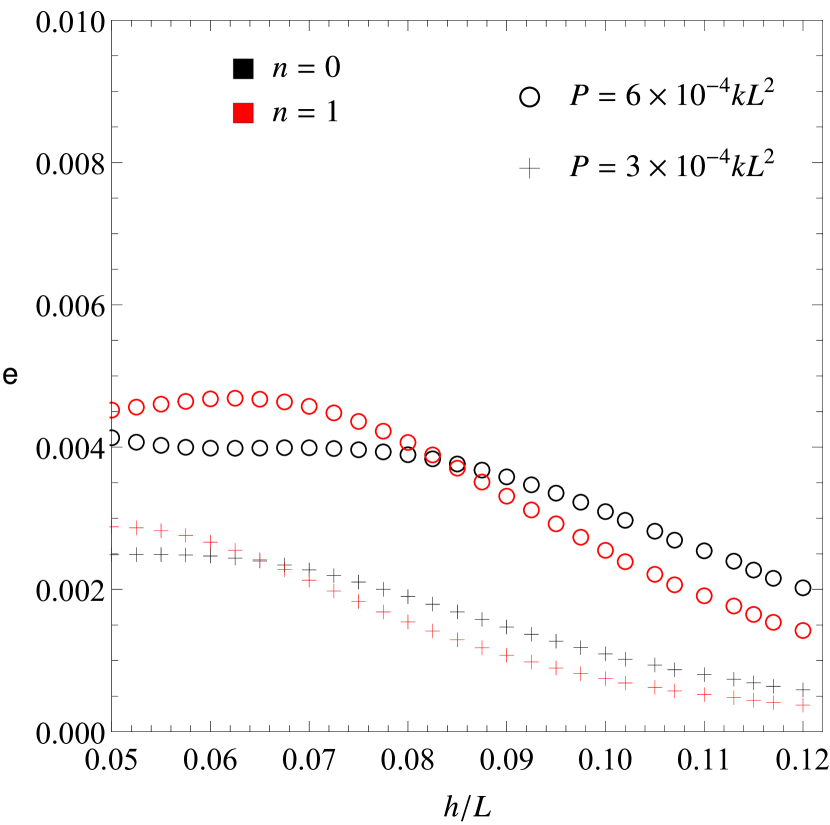
In the pulling experiment with the higher load the efficiencies observed are consistently higher than those for the lower load for all thicknesses. We also note that for the higher load, efficiencies for are also consistently higher than for . For the lower load, instead, the two efficiency curves cross at a critical thickness of approximately , above which efficiency is higher for than for . For the bending experiment, we observe that higher values of the dead load result in higher efficiencies for both and . However, for each value of the dead load, the same crossing in the efficiency curves seen for the lower load in the pulling experiment manifests itself: there are two critical thicknesses, and (for the lower and higher loads, respectively), above which the efficiency is again higher for than for .
Thus, if we may say that an increase in the applied load increases systematically the efficiency of thermal recovery, the role of the imprinted nematic texture is not so clear cut, as it seems to be also affected by the ribbon’s thickness. A general indication (independent of the applied load) seems to be that for sufficiently thin ribbons, non-uniformity in the imprinted nematic texture should grant a higher efficiency.
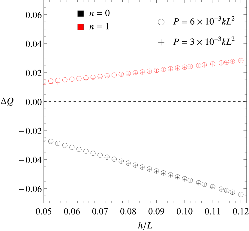
We also note that an increase in the value of from its value in the reference configuration requires heat to be extracted from the ribbon, whereas a decrease in requires heat to be injected. Figure 5(c) shows as a function of its normalized thickness in the activation process of the ribbon, starting from its mechanically fully pulled configuration. Computation of from (57) for the pulling experiment shows that for heat must be injected into the ribbon to recover work (i.e., ), whereas for , heat must be extracted (i.e., ). This observation is consistent with the fact that the order parameter had to be increased from its reference value for in order to recover work, whereas for it had to be decreased.
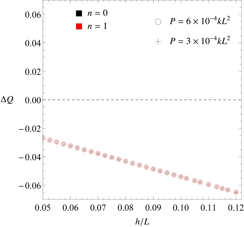
Figure 5(d) shows as a function of the normalized thickness of the ribbon for the bending experiment. In this case, for both and , heat must be extracted (i.e. ) from the ribbon to activate it in a fashion that the resulting deformation pulls back on the applied load. This is consistent with Fig. 4(b), where in the bending experiment the order parameter is increased from its base value in order to recover work. We also note that the numerical value of happens to be very close for and .
Figures 5(c) and 5(d) reveal that is practically unaffected by the load and it scales linearly with the thickness (that is, with the volume of the three-dimensional ribbon), in complete agreement with our (approximate) representation of the activation process a one traversing a sequence of equilibrium condensation states identified with the absolute minimizers of induced by compliant choices of in (23). This way of reasoning is further illuminated in Appendix A, where it is applied to a simplified setting.
VIII Conclusions
We computed the equilibrium configurations of a ribbon consisting of nematic polymer networks under the action of an external load. The numerical code that was instrumental to this end allowed us to depict the swirling configurations that the ribbon can achieve, most of them exhibiting various degrees of bending and twisting.
Our major interest lied in describing the mechanical behaviour of a ribbon activated under the persistent action of a load. In particular, we performed two numerical experiments: in one, the load pulled the ribbon; in the other, it bent it. In both experiments, we imprinted two different nematic textures in the reference configuration (which were conveyed by the ensuing deformations): one was uniform, the other was not. The activation of the material was devised in such a way that the spontaneous deformation induced by it would antagonize the applied load, so as to recover part of the work done by the latter. We defined the efficiency of the activation process as the ratio between the work recovered and the activation energy.
Our systematic explorations, as limited as they may appear, seem to support two conjectures about the activation efficiency of pre-loaded NPN ribbons, one more general than the other: (1) efficiency increases with the load, (2) non-uniformity in the imprinted nematic texture increases efficiency in sufficiently thin ribbons.
Further studies are needed to either prove or disprove these conjectures, as well as to evolve into dynamics the customary quasi-static approach to actuation adopted here.
Appendix A Toy model
Consider a system with a single mechanical variable, , and a single internal variable, . The internal energy of the system has two components, , which depends on both variables, and , which depends on and the value of that makes attain its absolute minimum, so that
| (58) |
Moreover, the power expended by an external (dead) load is given by , where a superimposed dot denotes differentiation with respect to time.
Equilibrium requires the function to be stationary, that is,
| (59) |
We denote by the pair of solutions to these equations corresponding to the absolute minimum of , assumed to exist. Both and will be regarded as functions of .
Now, we imagine a quasi-static process that takes the system through a set of equilibrium states parameterized by a curve . The first law of thermodynamics dictates that during this process the following equation be obeyed,
| (60) |
where is the energy supplied to the system per unit time (possibly in form of heat) to perform the process. In (60), both and depend on through . It follows from (60) that
| (61) |
Making use of (59) in (61), we readily obtain that
| (62) |
and integrating over the whole process, we finally arrive at
| (63) |
which delivers the total amount of energy that needs to be supplied to the system during the imagined process.
Equation (63) simplifies even further if we can assume that
| (64) |
which is exact when does not depend on . When (64) applies, the left-hand side of (62) is approximately a total derivative and (63) becomes
| (65) |
where is the increment (with sign) of the minimal value of during the whole process. When applied to a three-dimensional body, (65) implies that scales like the volume of the body, a conclusion confirmed by panels 5(c) and 5(d) of Fig. 5 in the main text.
As an easy application of (63), we consider the case of a linear spring with rest length , whose preferred value minimizes an internal potential . Here and play the role of and , respectively. We set
| (66) |
where is an elastic constant, is a material constant and is an increasing function. Simple calculations show that for this choice of functions (63) can be cast in the following equivalent form,
| (67) |
For example, for with , (66) shows that for a given amount of heat poured into a pulled spring (), the extension of the rest length produced by a process of quasistatic thermal expansion is larger than for a compressed spring ().
References
- Warner and Terentjev [2003] M. Warner and E. M. Terentjev, Liquid Crystal Elastomers, International Series of Monographs on Physics, Vol. 120 (Oxford University Press, New York, 2003).
- Mahimwalla et al. [2012] Z. Mahimwalla, K. G. Yager, J. ichi Mamiya, A. Shishido, A. Priimagi, and C. J. Barrett, Azobenzene photomechanics: prospects and potential applications, Polym. Bull. 69, 967 (2012).
- Ube and Ikeda [2014] T. Ube and T. Ikeda, Photomobile polymer materials with crosslinked liquid-crystalline structures: Molecular design, fabrication, and functions, Angew. Chem. Int. Ed. 53, 10290 (2014).
- White [2018] T. J. White, Photomechanical effects in liquid crystalline polymer networks and elastomers, J. Polym. Sci. Part B: Polym. Phys. 56, 695 (2018).
- Ula et al. [2018] S. W. Ula, N. A. Traugutt, R. H. Volpe, R. R. Patel, K. Yu, and C. M. Yakacki, Liquid crystal elastomers: an introduction and review of emerging technologies, Liquid Cryst. Rev. 6, 78 (2018).
- Pang et al. [2019] X. Pang, J.-a. Lv, C. Zhu, L. Qin, and Y. Yu, Photodeformable azobenzene-containing real polymers and soft actuators, Adv. Mater. 31, 1904224 (2019).
- Kuenstler and Hayward [2019] A. S. Kuenstler and R. C. Hayward, Light-induced shape morphing of thin films, Curr. Opin. Colloid & Interface Sci. 40, 70 (2019).
- Warner [2020] M. Warner, Topographic mechanics and applications of liquid crystalline solids, Annu. Rev. Condens. Matter Phys. 11, 125 (2020).
- Lagerwall [2023] J. Lagerwall, Liquid crystal elastomer actuators and sensors: Glimpses of the past, the present and perhaps the future, Programmable Materials 1, e9 (2023).
- Anderson et al. [1999] D. R. Anderson, D. E. Carlson, and E. Fried, A continuum-mechanical theory for nematic elastomers, J. Elast. 56, 33 (1999).
- Zhang et al. [2019] Y. Zhang, C. Xuan, Y. Jiang, and Y. Huo, Continuum mechanical modeling of liquid crystal elastomers as dissipative ordered solids, J. Mech. Phys. Solids 126, 285 (2019).
- Bai and Bhattacharya [2020] R. Bai and K. Bhattacharya, Photomechanical coupling in photoactive nematic elastomers, J. Mech. Phys. Solids 144, 104115 (2020).
- Mihai et al. [2021] L. A. Mihai, H. Wang, J. Guilleminot, and A. Goriely, Nematic liquid crystalline elastomers are aeolotropic materials, Proc. R. Soc. London A 477, 20210259 (2021).
- Korley and Ware [2021] L. T. J. Korley and T. H. Ware, Introduction to special topic: Programmable liquid crystal elastomers, J. Appl. Phys. 130, 220401 (2021).
- Hager et al. [2015] M. D. Hager, S. Bode, C. Weber, and U. S. Schubert, Shape memory polymers: Past, present and future developments, Prog. Polym. Sci. 49-50, 3 (2015).
- Wang et al. [2022] X. Wang, Y. He, Y. Liu, and J. Leng, Advances in shape memory polymers: Remote actuation, multi-stimuli control, 4d printing and prospective applications, Mater. Sci. Eng.: R: Reports 151, 100702 (2022).
- Modes et al. [2010] C. D. Modes, K. Bhattacharya, and M. Warner, Disclination-mediated thermo-optical response in nematic glass sheets, Phys. Rev. E 81, 060701 (2010).
- Corbett and Warner [2006] D. Corbett and M. Warner, Nonlinear photoresponse of disordered elastomers, Phys. Rev. Lett. 96, 237802 (2006).
- Corbett and Warner [2007] D. Corbett and M. Warner, Linear and nonlinear photoinduced deformations of cantilevers, Phys. Rev. Lett. 99, 174302 (2007).
- Corbett and Warner [2008] D. Corbett and M. Warner, Polarization dependence of optically driven polydomain elastomer mechanics, Phys. Rev. E 78, 061701 (2008).
- Korner et al. [2020] K. Korner, A. S. Kuenstler, R. C. Hayward, B. Audoly, and K. Bhattacharya, A nonlinear beam model of photomotile structures, Proc. Natl. Acad. Sci. USA 117, 9762 (2020).
- Goriely et al. [2023] A. Goriely, D. E. Moulton, and L. A. Mihai, A rod theory for liquid crystalline elastomers, J. Elast. 153, 509 (2023).
- Sonnet and Virga [2024] A. M. Sonnet and E. G. Virga, Model for a photoresponsive nematic elastomer ribbon, J. Elast. 155, 327 (2024).
- Cedeno Madera et al. [2024] R. Cedeno Madera, I. A. Diaz, M. Nait-Abdelaziz, and S. Aloise, Understanding the photomechanical effect in organic photoactuators: a comprehensive review of mechanical models and numerical simulations, Smart Mater. Struct. 33, 073006 (2024).
- Singh and Virga [2023a] H. Singh and E. G. Virga, A ribbon model for nematic polymer networks, J. Elast. 153, 613 (2023a).
- Ozenda et al. [2020] O. Ozenda, A. M. Sonnet, and E. G. Virga, A blend of stretching and bending in nematic polymer networks, Soft Matter 16, 8877 (2020).
- Bladon et al. [1994] P. Bladon, E. M. Terentjev, and M. Warner, Deformation-induced orientational transitions in liquid crystals elastomer, J. Phys. II France 4, 75 (1994).
- Warner et al. [1988] M. Warner, K. P. Gelling, and T. A. Vilgis, Theory of nematic networks, J. Chem. Phys. 88, 4008 (1988).
- Warner and Wang [1991] M. Warner and X. J. Wang, Elasticity and phase behavior of nematic elastomers, Macromolecules 24, 4932 (1991).
- Warner and Mostajeran [2018] M. Warner and C. Mostajeran, Nematic director fields and topographies of solid shells of revolution, Proc. R. Soc. Lond. A 474, 20170566 (2018).
- Ozenda and Virga [2021] O. Ozenda and E. G. Virga, On the Kirchhoff-Love hypothesis (revised and vindicated), J. Elast. 143, 359 (2021).
- Singh and Virga [2023b] H. Singh and E. G. Virga, Bending and stretching in a narrow ribbon of nematic polymer networks, J. Elast. 154, 531 (2023b).
- Zhou et al. [2019] B. Zhou, E. Bernhardt, A. Bhuyan, Z. Ghorbanishiadeh, N. Rasmussen, J. Lanska, and M. G. Kuzyk, Theoretical and experimental studies of photomechanical materials, J. Opt. Soc. Am. B 36, 1492 (2019).
- Antman [1995] S. S. Antman, Nonlinear Problems of Elasticity, Applied Mathematical Sciences, Vol. 107 (Springer, New York, 1995).
- Hornung [2010] P. Hornung, Euler-Lagrange equations for variational problems on space curves, Phys. Rev. E 81, 066603 (2010).
- Starostin and van der Heijden [2014] E. L. Starostin and G. H. M. van der Heijden, Theory of equilibria of elastic 2-braids with interstrand interaction, J. Mech. Phys. Solids 64, 83 (2014).
- Finkelmann et al. [2001] H. Finkelmann, A. Greve, and M. Warner, The elastic anisotropy of nematic elastomers, Eur. Phys. J. E 5, 281 (2001).
- Verwey et al. [1996] G. C. Verwey, M. Warner, and E. M. Terentjev, Elastic instability and stripe domains in liquid crystalline elastomers, J. Phys. II France 6, 1273 (1996).
- Nguyen and Selinger [2017] T.-S. Nguyen and J. V. Selinger, Theory of liquid crystal elastomers and polymer networks, Eur. Phys. J. E 40, 76 (2017).
- Maier and Saupe [1958] W. Maier and A. Saupe, Eine einfache molekulare Theorie des nematischen kristallinflüssigen Zustandes, Z. Naturforsch. 13a, 564 (1958).
- Maier and Saupe [2004] W. Maier and A. Saupe, A simple molecular theory of the nematic liquid-crystalline state, in Crystals that Flow: Classic Papers from the History of Liquid Crystals, edited by T. J. Sluckin, D. A. Dunmur, and H. Stegemeyer (Taylor & Francis, London, 2004) pp. 380–387.
- Sonnet and Virga [2012] A. M. Sonnet and E. G. Virga, Dissipative Ordered Fluids. Theories for Liquid Crystals (Springer, London, 2012).
- Dichmann et al. [1996] D. J. Dichmann, Y. Li, and J. H. Maddocks, Hamiltonian formulations and symmetries in rod mechanics, in Mathematical Approaches to Biomolecular Structure and Dynamics, The IMA Volumes in Mathematics and its Applications, edited by J. P. Mesirov, K. Schulten, and D. W. Sumners (Springer, New York, 1996) pp. 71–113.
- Champneys et al. [1997] A. R. Champneys, G. W. Hunt, J. M. T. Thompson, S. Kehrbaum, and J. H. Maddocks, Elastic rods, rigid bodies, quaternions and the last quadrature, Phil. Trans. R. Soc. London A 355, 2117 (1997).
- Altmann [1989] S. L. Altmann, Hamilton, Rodrigues, and the quaternion scandal, Math. Mag. 62, 291 (1989).
- Ascher and Petzold [1998] U. Ascher and L. Petzold, Computer Methods for Ordinary Differential Equations and Differential-Algebraic Equations (SIAM, Philadelphia, 1998).
- Doedel [2014] E. Doedel, Lecture Notes: An introduction to numerical continuation methods with applications (2014), https://users.encs.concordia.ca/~doedel/courses/comp-6361/slides.pdf.
- Allgower and Georg [2003] E. L. Allgower and K. Georg, Introduction to Numerical Continuation Methods, Classics in Applied Mathematics, Vol. 45 (SIAM, Philadelphia, 2003).
- Tajbakhsh and Terentjev [2001] A. Tajbakhsh and E. Terentjev, Spontaneous thermal expansion of nematic elastomers, Eur. Phys. J. E 6, 181 (2001).