Wasserstein Gradient Flows of MMD Functionals with Distance Kernel and Cauchy Problems on Quantile Functions

Abstract

We give a comprehensive description of Wasserstein gradient flows of maximum mean discrepancy (MMD) functionals $\mathcal{F}_{\nu}\coloneqq\text{MMD}_{K}^{2}(\cdot,\nu)$ towards given target measures $\nu$ on the real line, where we focus on the negative distance kernel $K(x,y)\coloneqq-|x-y|$. In one dimension, the Wasserstein-2 space can be isometrically embedded into the cone $\mathcal{C}(0,1)\subset L_{2}(0,1)$ of quantile functions leading to a characterization of Wasserstein gradient flows via the solution of an associated Cauchy problem on $L_{2}(0,1)$. Based on the construction of an appropriate counterpart of $\mathcal{F}_{\nu}$ on $L_{2}(0,1)$ and its subdifferential, we provide a solution of the Cauchy problem. For discrete target measures $\nu$, this results in a piecewise linear solution formula. We prove invariance and smoothing properties of the flow on subsets of $\mathcal{C}(0,1)$. For certain $\operatorname{\mathcal{F}}_{\nu}$-flows this implies that initial point measures instantly become absolutely continuous, and stay so over time. Finally, we illustrate the behavior of the flow by various numerical examples using an implicit Euler scheme and demonstrate differences to the explicit Euler scheme, which is easier to compute, but comes with limited convergence guarantees.

1 Introduction

Wasserstein gradient flows have been examined in stochastic analysis for a long time and recently received increasing interest in machine learning, leading to intriguing research questions that often fall outside the scope of the existing theory, see, e.g., [15, 23, 29]. In this paper, we concentrate on Wasserstein gradient flows of MMD functionals $\mathcal{F}_{\nu}\coloneqq\text{MMD}_{K}^{2}(\cdot,\nu)$ towards given target measures $\nu$. Wasserstein gradient flows of MMDs with smooth kernels $K$ like, e.g., the Gaussian one, preserve absolutely continuous measures as well as empirical measures, so that in the latter case, just the movement of particles has to be taken into account [2]. For non-smooth kernels like, e.g., the negative distance kernel, the properties of the measure can heavily vary during the flow. Figure 1 shows the simple example of a Wasserstein gradient flow on the line starting from an initial measure $\mu_{0}=\delta_{-1}$ towards the target measure $\nu=\delta_{0}$, where the behavior of the flow changes completely, see also Example 6.8.

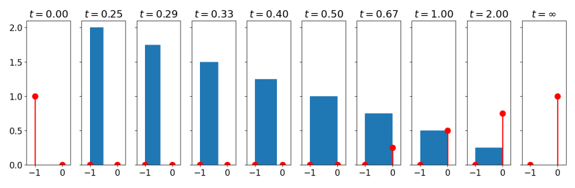
Figure 1: Wasserstein gradient flow of $\mathcal{F}_{\nu}$ from $\delta_{-1}$ towards $\nu=\delta_{0}$. The absolutely continuous part is visualized by its density in blue (area equals mass) and the atomic part by the red dotted vertical line (height equals mass). The flow changes immediately from a point measure to a uniform one with increasing support. It stays absolutely continuous until approaching the target support point $0$. Then it becomes the sum of an absolutely continuous measure and a discrete one, where the weight of the latter increases in time, see [24].

In general, the characterization of Wasserstein gradient flows of MMD functionals with non-smooth kernels appears to be complicated. For the interaction energy, which is only one part of the MMD functional, we refer to [25] and in relation with potential theory to [14]; for functionals which are the sum of the interaction energy and a potential energy from $\operatorname{\mathcal{C}}^{1}(\operatorname{\mathbb{R}}^{d})$ which are moreover geodesically convex, see [13]. Existence and global convergence results of MMD flows with the Coulomb kernel were proven in [8].

However, the flow examination can be simplified in one dimension, since in this case the Wasserstein spaces can be isometrically embedded into the cone $\mathcal{C}(0,1)\subset L_{2}(0,1)$ of quantile functions of measures. The flow of just the interaction energy, and also for a system of two interacting measures, was considered in [7, 12], see Remark 4.6. The recent preprint [20] investigates a non-local conservation law, where the interaction kernel is Lipschitz continuous and supported on the negative half line. Another special case, namely with a single point target measure was treated in [24]. Discretized versions of $\operatorname{\mathcal{F}}_{\nu}$ in the one-dimensional case and their convergence properties to the continuous setting were considered in [17, 18, 22]. Our work is also different from the recent article [27], where the functional is a porous-medium type approximation of the interaction energy for the Riesz (or Coulomb) kernel $-|x-y|^{r}$ with $r\in(-1,0)$, and the kernel $-|x-y|^{r}$ for $r>1$ but not $r=1$ is covered by the results in [11]. Further, connections between continuity equations and, more generally, scalar conservation laws in one dimension and their associated PDEs on quantile functions related to various Wasserstein-$p$ distances were explored, e.g., in [10, 21, 30], but focusing on the longtime behavior of solutions. Here, we refer to the overview paper [19].

In this paper, we consider the flow of the whole MMD functional with attraction term and repulsion term for arbitrary starting and target measures, concentrating on the negative distance kernel $K(x,y)\coloneqq-|x-y|$. Taking the isometric embedding into account, a functional $F_{\nu}$ on $\mathcal{C}(0,1)$ can be associated to the MMD functional $\operatorname{\mathcal{F}}_{\nu}$ on the Wasserstein space. We construct a continuous extension of this functional $F_{\nu}$ to the space $L_{2}(0,1)$ and compute its subdifferential. Then, starting with a measure $\mu_{0}$ with quantile function $Q_{\mu_{0}}$, we characterize the Wasserstein gradient flow of $\operatorname{\mathcal{F}}_{\nu}$ via $\gamma_{t}\coloneqq(g(t))_{\#}\Lambda_{(0,1)}$, where $g$ is the unique strong solution of the associated Cauchy problem on $L_{2}(0,1)$:

$$\begin{cases}\partial_{t}g(t)\in-\partial F_{\nu}(g(t)),\quad t\in(0,\infty),\\ g(0)=Q_{\mu_{0}}.\end{cases}$$

Indeed, the strong solution of the Cauchy problem exists and stays within the cone $\mathcal{C}(0,1)$, i.e., quantile functions remain quantile functions. We identify further interesting invariant subset of $\mathcal{C}(0,1)$, in which the $F_{\nu}$-flow remains once it has started there. In particular, we prove that the $F_{\nu}$-flow preserves continuity and Lipschitz properties of the initial datum $Q_{\mu_{0}}$ under suitable conditions on the target $Q_{\nu}$. This includes cases where point masses cannot form during the flow – in contrast to the example given by Figure 1. Also, the phenomenon, where initial point masses immediately explode into absolutely continuous measures, is covered by our smoothing result, see Theorem 6.5. This smoothing effect is driven by the repulsive nature of the interaction energy part of our MMD functional, see also [7, 12]. But note that in our case, the potential energy part in conjunction with a fixed target measure $\nu$ plays a fundamental role, whether or not this smoothing property can come into effect, and remain over time – see again Figure 1.

Moreover, we discuss the explicit pointwise solution $g_{s}$ of the Cauchy problem at continuity points $s\in(0,1)$ of the quantile function $Q_{\nu}$ and show that the family of these functions determines the solution of the Cauchy problem via $[g(t)](s)=g_{s}(t)$. Furthermore, based on Euler backward and forward schemes, we illustrate the flow by some numerical examples.

Outline of the paper.

In Section 2, we recall Wasserstein gradient flows, and especially flows on the line in Section 3. We take great care of the relation between quantile functions and cumulative density functions (CDFs) of probability measures and recall properties of maximal monotone operators on Hilbert spaces which we need later. Finally, we formulate our central characterization of Wasserstein gradient flows by the solution of a Cauchy problem in $L_{2}(0,1)$. The MMD and the functional $\operatorname{\mathcal{F}}_{\nu}\coloneqq\text{MMD}_{K}^{2}(\cdot,\nu)$ with the distance kernel is introduced in Section 4. We determine a continuous functional $F_{\nu}$ on $L_{2}(0,1)$ whose restriction to $\mathcal{C}(0,1)$ is associated with $\operatorname{\mathcal{F}}_{\nu}$, meaning that it fulfills $\operatorname{\mathcal{F}}_{\nu}(\mu)=F_{\nu}(Q_{\mu})$ for all measures $\mu$ in the Wasserstein space. We compute the subdifferential of $F_{\nu}$ and show that the related Cauchy problem produces indeed a flow that stays within the cone $\mathcal{C}(0,1)$. In Section 5, we provide a solution of the pointwise Cauchy problem and show that it also determines the overall solution. In particular, an explicit solution formula is given for discrete target measures $\nu$. Section 6 deals with invariance and smoothing properties of our gradient flows. We show that certain $F_{\nu}$-flows preserve (and improve) Lipschitz properties of the initial quantile $Q_{\mu_{0}}$ by describing the time evolution of the Lipschitz constants. Also, we prove for general targets $\nu$ that the support of the starting measure stays convex and grows monotonically. Finally, Section 7, briefly introduces Euler backward and forward schemes and illustrates properties of the flow by numerical examples. The appendix collects auxiliary and additional material.

2 Wasserstein Gradient Flows

Let $\mathcal{M}(\operatorname{\mathbb{R}}^{d})$ denote the space of $\sigma$-additive, signed Borel measures and $\mathcal{P}(\operatorname{\mathbb{R}}^{d})$ the set of probability measures on $\operatorname{\mathbb{R}}^{d}$. For $\mu\in\mathcal{M}(\operatorname{\mathbb{R}}^{d})$ and a measurable map $T\colon\operatorname{\mathbb{R}}^{d}\to\operatorname{\mathbb{R}}^{n}$, the push-forward of $\mu$ via $T$ is given by $T_{\#}\mu\coloneqq\mu\circ T^{-1}$. We consider the Wasserstein space $\operatorname{\mathcal{P}}_{2}(\operatorname{\mathbb{R}}^{d})\coloneqq\{\mu\in\operatorname{\mathcal{P}}(\operatorname{\mathbb{R}}^{d})\colon\int_{\operatorname{\mathbb{R}}^{d}}\|x\|_{2}^{2}\mathop{}\!\mathrm{d}\mu(x)<\infty\}$ equipped with the Wasserstein distance $W_{2}\colon\operatorname{\mathcal{P}}_{2}(\operatorname{\mathbb{R}}^{d})\times\operatorname{\mathcal{P}}_{2}(\operatorname{\mathbb{R}}^{d})\to[0,\infty)$,

$$W_{2}^{2}(\mu,\nu)\coloneqq\min_{\pi\in\Gamma(\mu,\nu)}\int_{\operatorname{\mathbb{R}}^{d}\times\operatorname{\mathbb{R}}^{d}}\|x-y\|_{2}^{2}\mathop{}\!\mathrm{d}\pi(x,y),\qquad\mu,\nu\in\operatorname{\mathcal{P}}_{2}(\operatorname{\mathbb{R}}^{d}),$$ (1)

where $\Gamma(\mu,\nu)\coloneqq\{\pi\in\operatorname{\mathcal{P}}_{2}(\operatorname{\mathbb{R}}^{d}\times\operatorname{\mathbb{R}}^{d}):(\pi_{1})_{\#}\pi=\mu,\;(\pi_{2})_{\#}\pi=\nu\}$ and $\pi_{i}(x)\coloneqq x_{i}$, $i=1,2$ for $x=(x_{1},x_{2})$, see e.g., [41, 42]. Further, $\|\cdot\|_{2}$ denotes the Euclidean norm on $\operatorname{\mathbb{R}}^{d}$. The set of optimal transport plans $\pi$ realizing the minimum in (1) is denoted by $\Gamma^{\rm{opt}}(\mu,\nu)$.

A curve $\gamma\colon I\to\operatorname{\mathcal{P}}_{2}(\operatorname{\mathbb{R}}^{d})$ on an interval $I\subset\operatorname{\mathbb{R}}$, is called a geodesic if there exists a constant $C\geq 0$ such that

$$W_{2}(\gamma_{t_{1}},\gamma_{t_{2}})=C|t_{2}-t_{1}|,\qquad\text{for all }t_{1},t_{2}\in I.$$ (2)

There also exists the notion of generalized geodesics, which in one dimension coincides with that of geodesics, so we do not introduce it here.

The Wasserstein space is a geodesic space, meaning that any two measures $\mu,\nu\in\operatorname{\mathcal{P}}_{2}(\operatorname{\mathbb{R}}^{d})$ can be connected by a geodesic. For $\lambda\in\operatorname{\mathbb{R}}$, a function $\operatorname{\mathcal{F}}\colon\operatorname{\mathcal{P}}_{2}(\operatorname{\mathbb{R}}^{d})\to(-\infty,\infty]$ is called $\lambda$-convex along geodesics if, for every $\mu,\nu\in\operatorname{dom}(\operatorname{\mathcal{F}})\coloneqq\{\mu\in\operatorname{\mathcal{P}}_{2}(\operatorname{\mathbb{R}}^{d}):\operatorname{\mathcal{F}}(\mu)<\infty\}$, there exists at least one geodesic $\gamma\colon[0,1]\to\operatorname{\mathcal{P}}_{2}(\operatorname{\mathbb{R}}^{d})$ between $\mu$ and $\nu$ such that

$$\operatorname{\mathcal{F}}(\gamma_{t})\leq(1-t)\,\operatorname{\mathcal{F}}(\mu)+t\,\operatorname{\mathcal{F}}(\nu)-\tfrac{\lambda}{2}\,t(1-t)\,W_{2}^{2}(\mu,\nu),\qquad t\in[0,1].$$ (3)

In the case $\lambda=0$, we just speak about convex functions.

Let $L_{2,\mu}$ denote the Bochner space of (equivalence classes of) functions $\xi:\operatorname{\mathbb{R}}^{d}\to\operatorname{\mathbb{R}}^{d}$ with $\|\xi\|_{L_{2,\mu}}^{2}\coloneqq\int_{\operatorname{\mathbb{R}}^{d}}\|\xi(x)\|_{2}^{2}\mathop{}\!\mathrm{d}\mu(x)<\infty$. The (regular) tangent space at $\mu\in\operatorname{\mathcal{P}}_{2}(\operatorname{\mathbb{R}}^{d})$ is given by

$${\text{T}}_{\mu}\mathcal{P}_{2}(\operatorname{\mathbb{R}}^{d}) \coloneqq\overline{\left\{\lambda(T-\text{Id}):(\text{Id},T)_{\#}\mu\in\Gamma^{\text{opt}}(\mu,T_{\#}\mu),\;\lambda>0\right\}}^{L_{2,\mu}}.$$ (4)

For a proper and lower semicontinuous (lsc) function $\operatorname{\mathcal{F}}\colon\operatorname{\mathcal{P}}_{2}(\operatorname{\mathbb{R}}^{d})\to(-\infty,\infty]$ and $\mu\in\operatorname{\mathcal{P}}_{2}(\operatorname{\mathbb{R}}^{d})$, the reduced Fréchet subdifferential $\partial\operatorname{\mathcal{F}}(\mu)$ at $\mu$ consists of all $\xi\in L_{2,\mu}$ satisfying

$$\operatorname{\mathcal{F}}(\nu)-\operatorname{\mathcal{F}}(\mu)\geq\inf_{\pi\in\Gamma^{\text{opt}}(\mu,\nu)}\int_{\operatorname{\mathbb{R}}^{2d}}\langle\xi(x),y-x\rangle\mathop{}\!\mathrm{d}\pi(x,y)+o(W_{2}(\mu,\nu))$$ (5)

for all $\nu\in\operatorname{\mathcal{P}}_{2}(\operatorname{\mathbb{R}}^{d})$.

A curve $\gamma\colon I\to\operatorname{\mathcal{P}}_{2}(\operatorname{\mathbb{R}}^{d})$ is (locally) $p$-absolutely continuous for $p\in[1,\infty]$ [1, Def. 1.1.1] if there exists a $m\in L_{p}(I,\operatorname{\mathbb{R}})$ (resp. $L_{p,\operatorname{loc}}(I,\operatorname{\mathbb{R}})$) such that

$$W_{2}(\gamma_{t},\gamma_{s})\leq\int_{s}^{t}m(r)\mathop{}\!\mathrm{d}{r}\qquad\text{for all }s,t\in I,s<t,$$

and we omit the $p$ if $p=1$. By [1, Thm. 8.3.1], if $\gamma$ is absolutely continuous, then there exists a Borel velocity field $v$ of functions $v_{t}\colon\operatorname{\mathbb{R}}^{d}\to\operatorname{\mathbb{R}}^{d}$ with with $\int_{I}\|v_{t}\|_{L_{2,\gamma_{t}}}\mathop{}\!\mathrm{d}t<\infty$ such that the continuity equation

$$\partial_{t}\gamma_{t}+\nabla_{x}\cdot(v_{t}\,\gamma_{t})=0$$ (6)

holds on $I\times\operatorname{\mathbb{R}}^{d}$ in the distributive sense, i.e., for all $\varphi\in C_{\mathrm{c}}^{\infty}(I\times\operatorname{\mathbb{R}}^{d})$ it holds

$$\int_{I}\int_{\operatorname{\mathbb{R}}^{d}}\partial_{t}\varphi(t,x)+v_{t}(x)\cdot\nabla_{x}\,\varphi(t,x)\mathop{}\!\mathrm{d}\gamma_{t}(x)\mathop{}\!\mathrm{d}{t}=0.$$ (7)

A locally $2$-absolutely continuous curve $\gamma\colon(0,\infty)\to\operatorname{\mathcal{P}}_{2}(\operatorname{\mathbb{R}}^{d})$ with velocity field $v_{t}\in\text{T}_{\gamma_{t}}\mathcal{P}_{2}(\operatorname{\mathbb{R}}^{d})$ is called Wasserstein gradient flow with respect to $\operatorname{\mathcal{F}}\colon\operatorname{\mathcal{P}}_{2}(\operatorname{\mathbb{R}}^{d})\to(-\infty,\infty]$ if

$$v_{t}\in-\partial\operatorname{\mathcal{F}}(\gamma_{t})\quad\text{for a.e. }t>0.$$ (8)

We have the following theorem which holds also true in $\operatorname{\mathbb{R}}^{d}$ when switching to so-called generalized geodesics, see [1, Thm. 11.2.1].

Theorem 2.1 (Existence and uniqueness of Wasserstein gradient flows).

Let $\operatorname{\mathcal{F}}\colon\operatorname{\mathcal{P}}_{2}(\operatorname{\mathbb{R}})\to(-\infty,\infty]$ be bounded from below, lower semicontinuous (lsc) and $\lambda$-convex along geodesics and $\mu_{0}\in\overline{\operatorname{dom}(\operatorname{\mathcal{F}})}$. Then there exists a unique Wasserstein gradient flow $\gamma\colon(0,\infty)\to\operatorname{\mathcal{P}}_{2}(\operatorname{\mathbb{R}})$ with respect to $\operatorname{\mathcal{F}}$ with $\gamma(0+)=\mu_{0}$. Furthermore, the piecewise constant curves constructed from the iterates of the minimizing movement scheme

$$\mu_{n+1}\coloneqq\operatorname*{arg\,min}_{\mu\in\operatorname{\mathcal{P}}_{2}(\operatorname{\mathbb{R}}^{d})}\Big{\{}\operatorname{\mathcal{F}}(\mu)+\frac{1}{2\tau}W_{2}^{2}(\mu_{n},\mu)\Big{\}},\qquad\tau>0,$$ (9)

i.e., $\gamma_{\tau}$ defined by $\gamma_{\tau}|_{(n\tau,(n+1)\tau]}\coloneqq\mu_{n}$, $n=0,1,\ldots$, converge locally uniformly to $\gamma$ as $\tau\downarrow 0$.

If $\lambda>0$, then $\operatorname{\mathcal{F}}$ admits a unique minimizer $\bar{\mu}\in\operatorname{\mathcal{P}}_{2}(\operatorname{\mathbb{R}})$ and we observe exponential convergence:

$$W_{2}(\gamma_{t},\bar{\mu})\leq e^{-\lambda t}W_{2}(\mu_{0},\bar{\mu})\quad\text{and}\quad\operatorname{\mathcal{F}}(\gamma_{t})-\operatorname{\mathcal{F}}(\bar{\mu})\leq e^{-2\lambda t}\big{(}\operatorname{\mathcal{F}}(\mu_{0})-\operatorname{\mathcal{F}}(\bar{\mu})\big{)}.$$

If $\lambda=0$ and $\bar{\mu}$ is a minimizer of $\operatorname{\mathcal{F}}$, then we have

$$\operatorname{\mathcal{F}}(\gamma_{t})-\operatorname{\mathcal{F}}(\bar{\mu})\leq\frac{1}{2t}W_{2}^{2}(\mu_{0},\bar{\mu}).$$

3 Wasserstein Gradient Flows in 1D

In the following, we recall that $\operatorname{\mathcal{P}}_{2}(\operatorname{\mathbb{R}})$ can be isometrically embedded into $L_{2}(0,1)$ via so-called quantile functions. This reduces Wasserstein gradient flows in one dimension to the consideration of gradient flows in the Hilbert space $L_{2}(0,1)$, or more precisely, in the cone of quantile functions. We will see in the main Theorem 3.5 of this section, that we have finally to deal with a Cauchy inclusion problem.

The cumulative distribution function (CDF) of $\nu\in\operatorname{\mathcal{P}}(\operatorname{\mathbb{R}})$ is given by

$$R_{\nu}^{+}\colon\operatorname{\mathbb{R}}\to[0,1],\quad R_{\nu}^{+}(x)\coloneqq\nu\big{(}(-\infty,x]\big{)},$$

and its quantile function by

$$Q_{\nu}\colon(0,1)\to\operatorname{\mathbb{R}},\quad Q_{\nu}(s)\coloneqq\min\{x\in\operatorname{\mathbb{R}}:R_{\nu}^{+}(x)\geq s\}.$$

Remark 3.1.

It is easy to check that $Q_{\mu}$ is strictly increasing if and only if $R_{\mu}^{+}$ is continuous. Further, $Q_{\mu}$ is continuous if and only if $R_{\mu}^{+}$ is strictly increasing on $\overline{(R_{\mu}^{+})^{-1}(0,1)}$.

We will also need the function

$$R_{\nu}^{-}\colon\operatorname{\mathbb{R}}\to[0,1],\quad R_{\nu}^{-}(x)\coloneqq\nu\big{(}(-\infty,x)\big{)}.$$

The functions $R_{\nu}^{+},R_{\nu}^{-}$ and $Q_{\nu}$ are monotonically increasing with only countably many discontinuities. They are visualized for a discrete measure in Fig. 2. For a nice overview on quantile functions in convex analysis, see also [36]. If $\nu(\{x\})=0$ for all $x\in\operatorname{\mathbb{R}}$, then the functions $R_{\nu}\coloneqq R_{\nu}^{-}=R_{\nu}^{+}$ are continuous. In general, the points of continuity $x\in\operatorname{\mathbb{R}}$ of $R_{\nu}^{+}$ and $R_{\nu}^{-}$ coincide, and there it holds $R_{\nu}^{-}(x)=R_{\nu}^{+}(x)$. Generally, we have $R_{\nu}^{-}\leq R_{\nu}^{+}$ such that

$$[R_{\nu}^{-}(x),R_{\nu}^{+}(x)]\neq\emptyset\hskip 11.38109pt\text{ for all }x\in\operatorname{\mathbb{R}}.$$

Both $R_{\nu}^{-}$ and $Q_{\nu}$ are left-continuous and, since they are increasing, also lower semicontinuous (lsc), whereas $R_{\nu}^{+}$ is right-continuous and, since it is increasing, upper semicontinuous (usc). Further, we have for $x\in\operatorname{\mathbb{R}}$ that

$$R_{\nu}^{+}(x)=\begin{cases}\max\{s\in(0,1):Q_{\nu}(s)\leq x\},&\text{if }x\in[\inf Q_{\nu}(s),\sup Q_{\nu}(s)),\\ 1,&\text{if }x\geq\sup Q_{\nu}(s),\\ 0,&\text{if }x<\inf Q_{\nu}(s),\end{cases}$$ (10)

where the infimum and supremum is taken over all $s\in(0,1)$, and

$$R_{\nu}^{-}(x)=\sup\{s\in(0,1):Q_{\nu}(s)<x\}\quad\text{for}\quad x>\inf_{s\in(0,1)}Q_{\nu}(s).$$ (11)

Note that formula (10) is different from an erroneous one in [36]. Moreover, it holds the Galois inequality, which states that

$$Q_{\nu}(s)\leq x\quad\text{if and only if}\quad s\leq R_{\nu}^{+}(x),$$ (12)

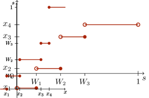
Figure 2: Functions $R_{\mu}^{+}$ (left), $R_{\mu}^{-}$ (middle) and $Q_{\mu}$ (right) for a discrete measure $\mu\coloneqq\sum_{k=1}^{4}w_{k}\delta_{x_{k}}$ with $W_{k}\coloneqq\sum_{j=1}^{k}w_{j}$.

The quantile functions of measures in $\mathcal{P}_{2}(\operatorname{\mathbb{R}})$ form a closed, convex cone

$$\mathcal{C}(0,1):=\{f\in L_{2}(0,1):f~{}\text{is increasing (a.e.)}\},$$

see also Remark A.1 in the appendix.

By the following theorem, see, e.g., [41, Thm. 2.18], the mapping $\mu\mapsto Q_{\mu}$ is an isometric embedding of $\operatorname{\mathcal{P}}_{2}(\operatorname{\mathbb{R}})$ into $L_{2}(0,1)$.

Theorem 3.2.

For $\mu,\nu\in\operatorname{\mathcal{P}}_{2}(\operatorname{\mathbb{R}})$, the quantile function $Q_{\mu}\in\mathcal{C}(0,1)$ satisfies $\mu=(Q_{\mu})_{\#}\Lambda_{(0,1)}$ with the Lebesgue measure $\Lambda$ on $(0,1)$ and

$$W_{2}^{2}(\mu,\nu)=\int_{0}^{1}|Q_{\mu}(s)-Q_{\nu}(s)|^{2}\mathop{}\!\mathrm{d}s.$$ (13)

Thus, instead of working with $\operatorname{\mathcal{F}}:\operatorname{\mathcal{P}}_{2}(\operatorname{\mathbb{R}})\to(-\infty,\infty]$, we can just deal with associated functions

$$F\colon L_{2}(0,1)\to(-\infty,\infty]\quad\text{with}\quad F(Q_{\mu})\coloneqq\operatorname{\mathcal{F}}(\mu).$$

Note that this relation determines $F$ only on $\mathcal{C}(0,1)$ and several extension to the whole space $L_{2}(0,1)$ are possible. One possibility would be to extend $F$ outside of $\mathcal{C}(0,1)$ by $\infty$. Yet, later in this work we will deal with a continuous extension of a specific functional which is everywhere finite on $L_{2}(0,1)$.

Now, instead of the (reduced) Fréchet subdifferential (5), we will use the regular subdifferential of functions $F\colon L_{2}(0,1)\to(-\infty,\infty]$ defined by

$$\partial F(u)\coloneqq\bigl{\{}v\in L_{2}(0,1):F(w)\geq F(u)+\langle v,w-u\rangle+o(\|w-u\|)\;~{}\text{for all }w\in L_{2}(0,1)\bigr{\}}.$$ (14)

If $F$ is convex, then the $o$-term can be skipped.

The following theorem collects well-known properties of subdifferential operators on Hilbert spaces [3]. Here, the domain of a multivalued operator $A\colon L_{2}(0,1)\to 2^{L_{2}(0,1)}$ is denoted by $\operatorname{dom}(A)\coloneqq\{u\in L_{2}(0,1):Au\neq\emptyset\}$.

Theorem 3.3.

Let $F:L_{2}(0,1)\to(-\infty,\infty]$ be proper and convex. Then $\partial F:L_{2}(0,1)\to 2^{L_{2}(0,1)}$ is a monotone operator, i.e. for every $u_{i}$ and $v_{i}\in\partial F(u_{i})$, $i=1,2$ it holds

$$\langle u_{1}-u_{2},v_{1}-v_{2}\rangle\geq 0.$$

If $F$ is in addition lsc, then $\partial F$ is maximal monotone and thus for any $\varepsilon>0$,

$$\text{{\rm Range}}(I+\varepsilon\partial F)=\bigcup\limits_{u\in L_{2}(0,1)}(I+\varepsilon\partial F)(u)=L_{2}(0,1).$$

Moreover, $\partial F$ is a closed operator, $\overline{\operatorname{dom}(F)}=\overline{\operatorname{dom}(\partial F)}$ and the resolvent

$$J_{\varepsilon}^{\partial F}\coloneqq(I+\varepsilon\partial F)^{-1}:L_{2}(0,1)\to L_{2}(0,1)$$

is single-valued.

Concerning the $\lambda$-convexity and lower semicontinuity of $\mathcal{F}$, we have the following proposition, whose proof is given in the appendix.

Proposition 3.4.

If $F:\mathcal{C}(0,1)\to(-\infty,\infty]$ is $\lambda$-convex, then $\mathcal{F}(\mu)\coloneqq F(Q_{\mu})$, $\mu\in\operatorname{\mathcal{P}}_{2}(\operatorname{\mathbb{R}})$, is $\lambda$-convex along geodesics. If $F$ is lsc, then the same holds true for $\mathcal{F}$.

The next theorem is central for our further considerations. It characterizes Wasserstein gradient flows by the solution of a Cauchy problem, where we have to ensure that the solution remains in the cone $\mathcal{C}(0,1)$. To this end, recall that given an operator $A:\operatorname{dom}(A)\subseteq L_{2}(0,1)\to 2^{L_{2}(0,1)}$ and an initial function $g_{0}\in L_{2}(0,1)$, a strong solution $g:[0,\infty)\to L_{2}(0,1)$ of the Cauchy problem

$$\begin{cases}\partial_{t}g(t)+Ag(t)~{}\ni~{}0,\quad t\in(0,\infty),\\ g(0)~{}=~{}g_{0},\end{cases}$$ (15)

is a function $g\in W^{1}_{1}\big{(}(0,T];L_{2}(0,1)\big{)}\cap C\big{(}[0,\infty);L_{2}(0,1)\big{)}$ for any $T>0$ which meets the initial condition and solves the differential inclusion in (15) pointwise for a.e. $t>0$, where $\partial_{t}g(t)$ denotes the strong derivative of $g$ at $t$.

Theorem 3.5.

Let $F\colon L_{2}(0,1)\to(-\infty,\infty]$ be a proper, convex and lsc function. Assume that for all (small) $\varepsilon>0$, the resolvent $J_{\varepsilon}^{\partial F}$ maps $\operatorname{\mathcal{C}}(0,1)$ into itself. Then, for any initial datum $g_{0}\in\mathcal{C}(0,1)\cap\operatorname{dom}(\partial F)$, the Cauchy problem

$$\begin{cases}\partial_{t}g(t)+\partial F(g(t))~{}\ni~{}0,\quad t\in(0,\infty),\\ g(0)~{}=~{}g_{0},\end{cases}$$ (16)

has a unique strong solution $g:[0,\infty)\to\mathcal{C}(0,1)$ which is expressible by the exponential formula

$$g(t)=\text{e}^{-t\partial F}g_{0}\coloneqq\lim_{n\to\infty}\left(I+\frac{t}{n}\partial F\right)^{-n}g_{0}.$$ (17)

The curve $\gamma_{t}\coloneqq(g(t))_{\#}\Lambda_{(0,1)}$ has quantile functions $Q_{\gamma_{t}}=g(t)$ and is a Wasserstein gradient flow of $\operatorname{\mathcal{F}}$ with $\gamma(0+)=(g_{0})_{\#}\Lambda_{(0,1)}$.

Proof.

1. By assumption, $\partial F$ is the subdifferential of a proper, convex and lsc function, and hence maximal monotone by Theorem 3.3. By standard results of semigroup theory, see e.g., Theorem A.2, there exists a strong solution $g:[0,\infty)\to L_{2}(0,1)$ of (16) satisfying the exponential formula (17). It remains to show that starting in $g_{0}\in\mathcal{C}(0,1)$, the solution remains in the cone $\mathcal{C}(0,1)$. Indeed, since $J_{\varepsilon}^{\partial F}$ maps $\operatorname{\mathcal{C}}(0,1)$ into itself, we can conclude that $\left(I+\frac{t}{n}\partial F\right)^{-n}g_{0}\in\mathcal{C}(0,1)$ for all $n\in\operatorname{\mathbb{N}}$. Since $\mathcal{C}(0,1)$ is closed in $L_{2}(0,1)$, this also holds true when the limit in (17) is taken, hence $g(t)\in\operatorname{\mathcal{C}}(0,1)$ for all $t\geq 0$.

2. Let $\gamma_{t}\coloneqq(g(t))_{\#}\Lambda_{(0,1)}$. First, we show that $\gamma$ is locally $2$-absolutely continuous. By Theorem A.2, the function $g$ is Lipschitz continuous, so there exists a $L>0$ such that for all $s,t\geq 0$ with $s<t$ we have

$$W_{2}(\gamma_{t},\gamma_{s})=\|g(t)-g(s)\|_{L_{2}(0,1)}\leq L(t-s)=\int_{s}^{t}L\mathop{}\!\mathrm{d}{\tau},$$

where the first equality is due to Theorem 3.2. Since the constant function $m\equiv L$ is in $L_{\infty}([0,\infty))$, the curve $\gamma\colon[0,\infty)\to(\operatorname{\mathcal{P}}_{2}(\operatorname{\mathbb{R}}),W_{2})$ is locally $2$-absolutely continuous.

Next, we show that the velocity field $v_{t}$ of $\gamma_{t}$ from (6) fulfills $v_{t}\in-\partial\operatorname{\mathcal{F}}(\gamma_{t})$. To calculate $v_{t}$, we exploit [1, Prop 8.4.6] stating that, for a.e. $t\in(0,\infty)$, the velocity field satisfies

$$0 =\lim_{\tau\downarrow 0}\frac{W_{2}(\gamma_{t+\tau},(\mathrm{Id}+\tau\,v_{t})_{\#}\gamma_{t})}{\tau}$$ (18)

$$=\lim_{\tau\downarrow 0}\frac{W_{2}(g(t+\tau)_{\#}\Lambda_{(0,1)},\bigl{(}g(t)+\tau\left(v_{t}\circ g(t)\right)\bigr{)}_{\#}\Lambda_{(0,1)})}{\tau}$$ (19)

Since $v_{t}\in\mathrm{T}_{\gamma_{t}}\mathcal{P}_{2}(\operatorname{\mathbb{R}}^{d})$, there exists a $\tilde{\tau}>0$ such that $(\operatorname{id},\operatorname{id}+\tilde{\tau}v_{t})_{\#}\gamma_{t}$ becomes an optimal transport plan. Moreover, [1, Lem 7.2.1] implies that the transport plans remain optimal for all $0<\tau\leq\tilde{\tau}$. For small $\tau>0$, the mappings $\operatorname{id}+\tau v_{t}$ are thus optimal and, especially, monotonically increasing. Consequently, the functions $g(t)+\tau(v_{t}\circ g(t))$ are also monotonically increasing, and their left-continuous representatives are quantile functions. Employing the isometry to $L_{2}(0,1)$, we hence obtain

$$0=\lim_{\tau\downarrow 0}\Big{\|}\frac{g(t+\tau)-g(t)}{\tau}-v_{t}\circ g(t)\Big{\|}_{L_{2}(0,1)}=\|\partial_{t}g(t)-v_{t}\circ g(t)\|_{L_{2}(0,1)}.$$ (20)

Thus, by construction (16) of $g$, we see that $v_{t}\circ g(t)\in-\partial F\left(g(t)\right)$ for a.e. $t$. In particular, for any $\mu\in\operatorname{\mathcal{P}}_{2}(\operatorname{\mathbb{R}})$, we obtain

$$0\,\leq\, F(Q_{\mu})-F\left(g(t)\right)+\int_{0}^{1}\left(v_{t}\circ g(t)\right)(s)\,\big{(}Q_{\mu}(s)-\left(g(t)\right)(s)\big{)}\mathop{}\!\mathrm{d}s$$ (21)

$$=\, \mathcal{F}(\mu)-\mathcal{F}(\gamma_{t})+\int_{\operatorname{\mathbb{R}}\times\operatorname{\mathbb{R}}}v_{t}(x)\,(y-x)\mathop{}\!\mathrm{d}\pi(x,y),$$ (22)

where $\pi\coloneqq(g(t),Q_{\mu})_{\#}\Lambda_{(0,1)}$. By Theorem 3.2, the plan $\pi$ is optimal between $\gamma_{t}$ and $\mu$, see also [41, Thm. 2.18]. By [31, Thm. 16.1(i),(ii)], we also know that $\pi$ is unique, so (5) yields that $v_{t}\in-\partial\operatorname{\mathcal{F}}(\gamma_{t})$. ∎

By the same arguments as in the proof of Theorem 3.5, we have the following corollary concerning invariant subsets of $\operatorname{\mathcal{C}}(0,1)$ of $F$-flows.

Corollary 3.6.

Let $D\subset\operatorname{\mathcal{C}}(0,1)$ be a closed subset and let $F\colon L_{2}(0,1)\to(-\infty,\infty]$ be a proper, convex and lsc function. Assume that for all (small) $\varepsilon>0$, the resolvent $J_{\varepsilon}^{\partial F}$ maps $D$ into itself. Then, the solution of the Cauchy problem (16) starting in $g_{0}\in D$ fulfills $g(t)\in D$ for all $t\geq 0$.

4 Flows of MMD with Distance Kernel

In this paper, we are mainly interested in Wasserstein gradient flows of MMD functionals $\mathcal{F}_{\nu}:\operatorname{\mathcal{P}}_{2}(\operatorname{\mathbb{R}})\to[0,\infty)$ for the negative distance kernel. After introducing these functionals, we will define an associated functional $F_{\nu}:L_{2}(0,1)\to\operatorname{\mathbb{R}}$ with $F_{\nu}(Q_{\mu})=\mathcal{F}_{\nu}(\mu)$. More precisely, we will extend $F_{\nu}$ from $\mathcal{C}(0,1)$ to $L_{2}(0,1)$ such that its subdifferential can be easily computed.

MMDs are defined with respect to kernels $K\colon\operatorname{\mathbb{R}}^{d}\times\operatorname{\mathbb{R}}^{d}\to\operatorname{\mathbb{R}}$. In this paper, we are interested in the negative distance kernel

$$K(x,y)\coloneqq-|x-y|,$$ (23)

which is symmetric and conditionally positive definite of order one. Then we define

$$\text{MMD}_{K}^{2}(\mu,\nu) \coloneqq\frac{1}{2}\int_{\operatorname{\mathbb{R}}^{d}\times\operatorname{\mathbb{R}}^{d}}K(x,y)\mathop{}\!\mathrm{d}\mu(x)\mathop{}\!\mathrm{d}\mu(y)-\int_{\operatorname{\mathbb{R}}^{d}\times\operatorname{\mathbb{R}}^{d}}K(x,y)\mathop{}\!\mathrm{d}\mu(x)\mathop{}\!\mathrm{d}\nu(y)$$ (24)

$$\quad+\frac{1}{2}\int_{\operatorname{\mathbb{R}}^{d}\times\operatorname{\mathbb{R}}^{d}}K(x,y)\mathop{}\!\mathrm{d}\nu(x)\mathop{}\!\mathrm{d}\nu(y).$$ (25)

The square root of the above formula defines a distance on $\operatorname{\mathcal{P}}_{2}(\operatorname{\mathbb{R}}^{d})$ for many kernels of interest including the negative distance kernel (23). In particular, we have that $\text{MMD}_{K}(\mu,\nu)\geq 0$ with equality if and only if $\mu=\nu$. Fixing the target measure $\nu$, the third summand becomes a constant and we may consider the MMD functional

$$\operatorname{\mathcal{F}}_{\nu}(\mu)\coloneqq\frac{1}{2}\int_{\operatorname{\mathbb{R}}^{d}\times\operatorname{\mathbb{R}}^{d}}K(x,y)\mathop{}\!\mathrm{d}\mu(x)\mathop{}\!\mathrm{d}\mu(y)-\int_{\operatorname{\mathbb{R}}^{d}\times\operatorname{\mathbb{R}}^{d}}K(x,y)\mathop{}\!\mathrm{d}\mu(x)\mathop{}\!\mathrm{d}\nu(y).$$ (26)

The first summand is known as interaction energy, while the second one is called potential energy of $V_{\nu}\coloneqq\int_{\operatorname{\mathbb{R}}^{d}}K(\cdot,y)\,\mathop{}\!\mathrm{d}\nu(y)$.

In the following, we are exclusively interested in $d=1$ and the negative distance kernel (23). Note that the MMD of the negative distance kernel is also known as energy distance [39, 40] and that in one dimension we have a relation to the Cramer distance

$$\mathrm{MMD}_{K}^{2}(\mu,\nu)=\int_{-\infty}^{\infty}(R_{\mu}(x)-R_{\nu}(x))^{2}\mathop{}\!\mathrm{d}x,$$

see [38, 26]. More precisely, we will deal with Wasserstein gradient flows of

$$\operatorname{\mathcal{F}}_{\nu}(\mu)=-\frac{1}{2}\int_{\operatorname{\mathbb{R}}\times\operatorname{\mathbb{R}}}|x-y|\mathop{}\!\mathrm{d}\mu(x)\mathop{}\!\mathrm{d}\mu(y)+\int_{\operatorname{\mathbb{R}}\times\operatorname{\mathbb{R}}}|x-y|\mathop{}\!\mathrm{d}\mu(x)\mathop{}\!\mathrm{d}\nu(y).$$ (27)

In dimensions $d\geq 2$, neither the interaction energy nor the whole $\text{MMD}_{K}^{2}$ functional with the negative distance kernel are $\lambda$-convex along geodesics, see [25], so that Theorem 2.1 does not apply. We will see that this is different on the real line. Note that in 1D, but not in higher dimensions, $\lambda$-convexity along geodesics implies the stronger property of $\lambda$-convexity along so-called generalized geodesics.

Next, we propose an associated functional of (27) on $L_{2}(0,1)$, which is determined on $\mathcal{C}(0,1)$ by $\mathcal{F}_{\nu}(\mu)=F_{\nu}(Q_{\mu})$. We consider the functional $F_{\nu}\colon L_{2}(0,1)\to\operatorname{\mathbb{R}}$ defined by

$$F_{\nu}(u) \coloneqq\int_{0}^{1}\left((1-2s)\big{(}u(s)-Q_{\nu}(s)\big{)}+\int_{0}^{1}|u(s)-Q_{\nu}(t)|\mathop{}\!\mathrm{d}{t}\right)\mathop{}\!\mathrm{d}{s}$$ (28)

$$=\int_{0}^{1}f\left(s,u(s)\right)\mathop{}\!\mathrm{d}{s},$$ (29)

where $f\colon(0,1)\times\operatorname{\mathbb{R}}\to\operatorname{\mathbb{R}}$ is given by

$$f(s,u)\coloneqq(1-2s)\big{(}u-Q_{\nu}(s)\big{)}+H(u),\quad H(u)\coloneqq\int_{0}^{1}|u-Q_{\nu}(t)|\mathop{}\!\mathrm{d}{t}.$$ (30)

Indeed, by the following lemma, whose proof can be found in [24], the functional $F_{\nu}$ is associated to $\mathcal{F}_{\nu}$.

Lemma 4.1.

For $\operatorname{\mathcal{F}}_{\nu}$ in (27), the functional $F_{\nu}\colon L_{2}(0,1)\to\operatorname{\mathbb{R}}$ defined by (28) fulfills $F_{\nu}(Q_{\mu})=\operatorname{\mathcal{F}}_{\nu}(\mu)$ for all $\mu\in\operatorname{\mathcal{P}}_{2}(\operatorname{\mathbb{R}})$.

By the next lemma, whose proof is given in the appendix, the functional $F_{\nu}$ has further desirable properties.

Lemma 4.2.

The functional $F_{\nu}\colon L_{2}(0,1)\to\operatorname{\mathbb{R}}$ in (28) is convex and continuous.

The subdifferential of $F_{\nu}$ can be computed explicitly.

Lemma 4.3 (Subdifferential of $F_{\nu}$).

For $u\in L_{2}(0,1)$, it holds

$$\partial F_{\nu}(u) =\big{\{}f\in L_{2}(0,1):$$ (31)

$$\quad\;\;f(s)\in 2\big{[}R_{\nu}^{-}\big{(}u(s)\big{)},R_{\nu}^{+}\big{(}u(s)\big{)}\big{]}-2s~{}\text{for a.e.}\;s\in(0,1)\big{\}}.$$ (32)

In particular, we have $\operatorname{dom}(\partial F_{\nu})=L_{2}(0,1)$.

Proof.

It holds $h\in\partial F_{\nu}(u)$ if and only if

$$h(s)\in\partial\big{[}f(s,\cdot)\big{]}\big{(}u(s)\big{)}\quad\text{for a.e. }s\in(0,1),$$

see, e.g., [35, Cor. 1B] or [37, Thm. 10.39]. Now,

$$\partial\big{[}f(s,\cdot)\big{]}(u)=(1-2s)+\partial H(u),$$ (33)

so that it remains to consider the second summand. Recall that for the convex, one-dimensional function $H$, we have $\partial H(u)=[D_{-}H(u),D_{+}H(u)]$ with the one-sided derivatives

$$D_{\pm}H(u)\coloneqq\lim_{\lambda\downarrow 0}\frac{H(u\pm\lambda)-H(u)}{\lambda}.$$

Let $h_{t}(u)\coloneqq|u-Q_{\nu}(t)|$ in the definition (30) of $H$. Then we conclude by Lebesgue’s dominated convergence theorem that

$$D_{\pm}H(u) =\lim_{\lambda\downarrow 0}\frac{H(u\pm\lambda)-H(u)}{\lambda}=\lim_{\lambda\downarrow 0}\int_{0}^{1}\frac{h_{t}(u\pm\lambda)-h_{t}(u)}{\lambda}\mathop{}\!\mathrm{d}t$$ (34)

$$=\int_{0}^{1}\lim_{\lambda\downarrow 0}\frac{h_{t}(u\pm\lambda)-h_{t}(u)}{\lambda}\mathop{}\!\mathrm{d}t=\int_{0}^{1}D_{\pm}h_{t}(u)\mathop{}\!\mathrm{d}t,$$ (35)

and consequently

$$\partial H(u)=\Bigl{[}\int_{0}^{1}D_{-}h_{t}(u)\mathop{}\!\mathrm{d}t,\int_{0}^{1}D_{+}h_{t}(u)\mathop{}\!\mathrm{d}t\Bigr{]}.$$ (36)

Next, we have

$$D_{-}h_{t}(u) =D_{+}h_{t}(u)=1\qquad\;\;\;\text{if }u>Q_{\nu}(t),$$

$$D_{-}h_{t}(u) =D_{+}h_{t}(u)=-1\qquad\,\text{if }u<Q_{\nu}(t),$$

$$D_{-}h_{t}(u) =-1,\;D_{+}h_{t}(u)=1\quad\text{if }u=Q_{\nu}(t),$$

so that we obtain by (10) and (11) the value

$$\int_{0}^{1}D_{-}h_{t}(u)\mathop{}\!\mathrm{d}t=\int_{0}^{R_{\nu}^{-}(u)}1\mathop{}\!\mathrm{d}{t}+\int_{R_{\nu}^{-}(u)}^{R_{\nu}^{+}(u)}-1\mathop{}\!\mathrm{d}{t}+\int_{R_{\nu}(u)^{+}}^{1}-1\mathop{}\!\mathrm{d}{t}=2R_{\nu}^{-}(u)-1$$

and similarly $\int_{0}^{1}D_{+}h_{t}(u)\mathop{}\!\mathrm{d}t=2R_{\nu}^{+}(u)-1$. This implies

$$\partial H(u)=2[R_{\nu}^{-}(u),R_{\nu}^{+}(u)]-1$$ (37)

and by (33) finally

$$\partial\big{[}f(s,\cdot)\big{]}(u)=2\big{[}R_{\nu}^{-}\big{(}u(s)\big{)},R_{\nu}^{+}\big{(}u(s)\big{)}\big{]}-2s.\qed$$

By the following lemma, $J_{\varepsilon}^{\partial F_{\nu}}$ fulfills the invariance condition from Theorem 3.5.

Lemma 4.4.

Let $F_{\nu}$ be defined by (28). Then, $J_{\varepsilon}^{\partial F_{\nu}}$ maps $\operatorname{\mathcal{C}}(0,1)$ into itself for all $\varepsilon>0$.

Proof.

Let $\varepsilon>0$ be arbitrarily fixed and $h\in\operatorname{\mathcal{C}}(0,1)$. By Theorem 3.3 and Lemma 4.2, we have that $\operatorname{Range}(I+\frac{\varepsilon}{2}\partial F_{\nu})=L_{2}(0,1)$, so we obtain the existence of $u\in L_{2}(0,1)$ fulfilling $h\in\left(I+\frac{\varepsilon}{2}\partial F_{\nu}\right)u$. The explicit representation of $\partial F_{\nu}$ in Lemma 4.3 yields

$$u(s)+\varepsilon[R_{\nu}^{-}(u(s)),R_{\nu}^{+}(u(s))]~{}\ni~{}h(s)+\varepsilon s\hskip 8.53581pt\text{ for a.e. }s\in(0,1).$$ (38)

We have to show that $u\in\operatorname{\mathcal{C}}(0,1)$. Since $h+\varepsilon(\cdot)\in\operatorname{\mathcal{C}}(0,1)$, there exists a null set $\operatorname{\mathcal{N}}\subset(0,1)$ such that outside of $\operatorname{\mathcal{N}}$, $h+\varepsilon(\cdot)$ is increasing and (38) holds. Assume that $u\notin\operatorname{\mathcal{C}}(0,1)$. Then, there exist $s_{1},s_{2}\in(0,1)$ outside of $\operatorname{\mathcal{N}}$ with $s_{1}<s_{2}$ and $u(s_{1})>u(s_{2})$. But since $R_{\nu}^{-}(u(s_{1}))-R_{\nu}^{+}(u(s_{2}))=\nu((u(s_{2}),u(s_{1}))\geq 0$, it follows that

$$h(s_{1})+\varepsilon s_{1}\geq u(s_{1})+\varepsilon R_{\nu}^{-}(u(s_{1}))>u(s_{2})+\varepsilon R_{\nu}^{+}(u(s_{2}))\geq h(s_{2})+\varepsilon s_{2},$$

contradicting that $h+\varepsilon(\cdot)$ is increasing outside of $\operatorname{\mathcal{N}}$, and the proof is finished. ∎

Combining the results from Lemmas 4.2 and 4.4, we can apply Theorem 3.5 to $F_{\nu}$. By Proposition 3.4, the properties of $F_{\nu}$ carry over to $\mathcal{F}_{\nu}$, thus Theorem 2.1 applies to $\operatorname{\mathcal{F}}_{\nu}$. Together, we obtain the following theorem.

Theorem 4.5.

Let $\mathcal{F}_{\nu}$ and $F_{\nu}$ be defined by (27) and (28), respectively. Then the Cauchy problem

$$\begin{cases}\partial_{t}g(t)\in-\partial F_{\nu}(g(t)),\quad t\in(0,\infty),\\ g(0)=Q_{\mu_{0}},\end{cases}$$ (39)

has a unique strong solution $g$, and the associated curve $\gamma_{t}\coloneqq(g(t))_{\#}\Lambda_{(0,1)}$ is the unique Wasserstein gradient flow of $\mathcal{F}_{\nu}$.

Finally, let us briefly have a look at the results of the paper [7] (based on [6]) concerning only the interaction energy part of the MMD functional.

Remark 4.6.

The authors of [7] showed a similar result as Theorem 4.5, but only for the interaction energy part $\mathcal{E}(\mu)=\frac{1}{2}\int_{\operatorname{\mathbb{R}}^{d}\times\operatorname{\mathbb{R}}^{d}}K(x,y)\mathop{}\!\mathrm{d}\mu(x)\mathop{}\!\mathrm{d}\mu(y)$ of the MMD (24). More precisely, they derived two equivalent criteria for a curve $\gamma\colon(0,\infty)\to\operatorname{\mathcal{P}}_{2}(\operatorname{\mathbb{R}})$ to be a Wasserstein gradient flow with respect to $\mathcal{E}$. The first characterization is that the distributions functions $R_{t}\coloneqq R_{\gamma(t)}^{+}$ solve

$$\partial_{t}R_{t}(x)+\partial_{x}(R_{t}^{2}(x)-R_{t}(x))=0$$

subject to some minimum entropy condition. Second, this can be characterized via quantile functions. That is, $\gamma$ is a Wasserstein gradient flow with respect to $\mathcal{E}$ if and only if its quantile functions $Q_{t}\coloneqq Q_{\gamma(t)}$ solve the $L_{2}$-subgradient inclusion

$$-\frac{\mathop{}\!\mathrm{d}}{\mathop{}\!\mathrm{d}t}Q_{t}\in\partial E(Q_{t}),\quad\text{where}\quad E(g)=\begin{cases}\int_{0}^{1}(1-2s)g(s)\mathop{}\!\mathrm{d}{s},&\text{if }g\in\operatorname{\mathcal{C}}(0,1),\\ \infty,&\text{otherwise,}\end{cases}$$

for almost every $t>0$. Based on this representation, they can explicitly compute the Wasserstein gradient flow with respect to $\mathcal{E}$ via the quantile function $Q_{\gamma(t)}(s)=Q_{\gamma(0)}(s)+t(2s-1)$ and prove that $\gamma(t)$ is absolutely continuous for all $t>0$. These results were extended in [12], where the authors consider gradient flows for the functional $\mathrm{MMD}_{K}^{2}\colon\operatorname{\mathcal{P}}_{2}(\operatorname{\mathbb{R}})\times\operatorname{\mathcal{P}}_{2}(\operatorname{\mathbb{R}})\to\operatorname{\mathbb{R}}$ and the related PDE system. In contrast to our setting, these gradient flows are defined on $\operatorname{\mathcal{P}}_{2}(\operatorname{\mathbb{R}})\times\operatorname{\mathcal{P}}_{2}(\operatorname{\mathbb{R}})$, i.e., they consider two interacting measures (species), while on our side, the second entry is fixed as the target measure $\nu$. Using again the embedding of the Wasserstein space into $L^{2}(0,1)$, they prove that gradient flows exist and that they remain absolutely continuous whenever the initial measures are absolutely continuous. Stability of stationary states of singular interaction energies and differentiable potentials on $\operatorname{\mathbb{R}}$ with bounded, compactly supported initial data is studied in [21].

5 Explicit Solution of the Cauchy Problem

Having the subdifferential of $F_{\nu}$ in (31) in mind, we first aim to find a solution of the pointwise Cauchy problem, i.e., for fixed $s\in(0,1)$ we are interested in

$$\begin{cases}\partial_{t}g_{s}(t)\in 2s-2[R_{\nu}^{-}(g_{s}(t)),R_{\nu}^{+}(g_{s}(t))],\quad\text{for a.e. }\;t>0,\\ g_{s}(0)=Q_{\mu_{0}}(s),\end{cases}$$ (40)

satisfying $g_{s}(t)=[g(t)](s)$. Since the proposed method works in the same way for the left- and right-continuous version of the CDF, we use $R_{\nu}^{\pm}$ to indicate one of them.

Lemma 5.1 (Pointwise solution).

Let $\nu,\mu_{0}\in\operatorname{\mathcal{P}}_{2}(\operatorname{\mathbb{R}})$. For any fixed continuity point $s\in(0,1)$ of $Q_{\nu}$, the curve

$$g_{s}(t)\coloneqq\begin{cases}\Phi_{\nu,s}^{-1}\big{(}2t\big{)},&t<T_{s},\\ Q_{\nu}(s),&\text{otherwise},\end{cases}$$ (41)

is a strong solution of (40), where $T_{s}\coloneqq\frac{1}{2}\Phi_{\nu,s}\left(Q_{\nu}(s)\right)$ and

$$\Phi_{\nu,s}(x)\coloneqq\int_{Q_{\mu_{0}}(s)}^{x}\left(s-R_{\nu}^{\pm}(z)\right)^{-1}\mathop{}\!\mathrm{d}z$$

with $x\in[\min\{Q_{\mu_{0}}(s),Q_{\nu}(s)\},\max\{Q_{\mu_{0}}(s),Q_{\nu}(s)\}]$. In particular, the inclusion in (40) holds true for every $t\in(0,\infty)$, where $\dot{g}_{s}(t)$ exists.

Proof.

1. First, assume that $s\in(0,1)$ is any point such that $Q_{\mu_{0}}(s)<Q_{\nu}(s)$. Since $R^{-}\leq R^{+}$ and by the Galois inequality (12), we have for any $z<Q_{\nu}(s)$ that $R_{\nu}^{\pm}(z)<s$. Hence $\left(s-R_{\nu}^{\pm}(z)\right)^{-1}$ exists and $\Phi_{\nu,s}(x)$ is finite for all $x<Q_{\nu}(s)$. For $x=Q_{\nu}(s)$ we distinguish two cases.
Case 1: $\Phi_{\nu,s}(Q_{\nu}(s))=\infty$. Fix any $\hat{x}<Q_{\nu}(s)$. Then, $\Phi_{\nu,s}:[Q_{\mu_{0}}(s),\hat{x}]\to[0,\infty)$ is absolutely continuous, and its derivative exists a.e. and is given by

$$\Phi_{\nu,s}^{\prime}(x)=\left(s-R_{\nu}^{\pm}(x)\right)^{-1}>0,\quad\text{for a.e. }x\in[Q_{\mu_{0}}(s),\hat{x}].$$

By a result of Zareckii [4, 33], the function $\Phi_{\nu,s}:[Q_{\mu_{0}}(s),\hat{x}]\to[0,\Phi_{\nu,s}(\hat{x})]$ is invertible, and its inverse is also absolutely continuous with derivative

$$(\Phi_{\nu,s}^{-1})^{\prime}(t)=\frac{1}{\Phi_{\nu,s}^{\prime}(\Phi_{\nu,s}^{-1}(t))}=s-R_{\nu}^{\pm}(\Phi_{\nu,s}^{-1}(t)),\quad\text{for a.e. }t\in[0,\Phi_{\nu,s}(\hat{x})].$$

Hence, by definition (41), the function $g_{s}$ is absolutely continuous on $[0,\frac{1}{2}\Phi_{\nu,s}(\hat{x}))$, and it holds

$$\dot{g}_{s}(t)=2s-2R_{\nu}^{\pm}(g_{s}(t)),\quad\text{for a.e. }t\in[0,\frac{1}{2}\Phi_{\nu,s}(\hat{x})).$$ (42)

Considering the above arguments, we notice that $g_{s}$ is differentiable at $t$ if and only if $g_{s}(t)$ is a continuity point of $R_{\nu}^{\pm}$, i.e. $R_{\nu}^{+}(g_{s}(t))=R_{\nu}^{-}(g_{s}(t))$. Since $\Phi_{\nu,s}(\hat{x})\uparrow\infty$ for $\hat{x}\uparrow Q_{\nu}(s)$, we see that $g_{s}$ is a strong solution of (40).
Case 2: $\Phi_{\nu,s}(Q_{\nu}(s))<\infty$. Then above arguments with $\hat{x}=Q_{\nu}(s)$ show that $g_{s}$ is absolutely continuous on $[0,T_{s})$, and it holds

$$\dot{g}_{s}(t)=2s-2R_{\nu}^{\pm}(g_{s}(t)),\quad\text{for a.e. }t\in[0,T_{s}).$$ (43)

By the continuity of $\Phi_{\nu,s}^{-1}:[0,2T_{s}]\to[Q_{\mu_{0}}(s),Q_{\nu}(s)]$ and by construction of $g_{s}$, we conclude that $g_{s}$ is continuous in $T_{s}$. Since $g_{s}\equiv Q_{\nu}(s)$ on $[T_{s},\infty)$, it is absolutely continuous on the whole half-line $[0,\infty)$. On the one hand, (12) immediately yields $s\leq R_{\nu}^{+}(Q_{\nu}(s))$, and on the other hand, its negation $s>R_{\nu}^{+}(x)\geq R_{\nu}^{-}(x)$ for $x<Q_{\nu}(s)$ implies $s\geq R_{\nu}^{-}(Q_{\nu}(s))$ due to the left-continuity of $R_{\nu}^{-}$. For this reason, we finally have

$$\dot{g}_{s}(t)=0\in 2s-2[R_{\nu}^{-}(Q_{\nu}(s)),R_{\nu}^{+}(Q_{\nu}(s))]\quad\text{for all }t\in[T_{s},\infty),$$ (44)

which means that $g_{s}$ is a strong solution of (40).
2. Next, assume that $s\in(0,1)$ is a continuity point of $Q_{\nu}$ such that $Q_{\mu_{0}}(s)>Q_{\nu}(s)$. Then Galois inequality (12) together with the fact that $s$ is a continuity point of $Q_{\nu}$ implies for $z>Q_{\nu}(s)$ that $R_{\nu}^{\pm}(z)>s$. Now, the rest follows analogously as in the first part.
3. For the case $Q_{\mu_{0}}(s)=Q_{\nu}(s)$, we clearly get the constant solution, and the proof is done. ∎

Next we show that the curve $g:[0,\infty)\to\mathcal{C}(0,1)$ is differentiable almost everywhere and solves the original $L_{2}$ problem (39).

Theorem 5.2 ($L_{2}$ solution).

The family

$$\{g_{s}\text{ in }\eqref{eq:expl-sol}\colon\,s\in(0,1)\;\text{ is a continuity point of }\;Q_{\nu}\}$$ (45)

strongly solves (39) via $[g(t)](s)\coloneqq g_{s}(t)$.

Proof.

Since (41) is a strong solution of (40), it holds for a.e. $t>0$ that

$$\lvert\dot{g}_{s}(t)\rvert\leq\lvert 2s-2R_{\nu}^{\pm}(g_{s}(t))\rvert\leq 4.$$

Since $g_{s}$ is absolutely continuous in $t$, this implies that $g_{s}:[0,\infty)\to\operatorname{\mathbb{R}}$ is Lipschitz continuous for a.e. fixed $s\in(0,1)$, and therefore, $g:[0,\infty)\to L_{2}(0,1)$ is Lipschitz continuous. In particular, $g$ is differentiable at a.e. $t>0$, i.e., for any differentiability point $\hat{t}>0$ outside a null set, the sequence of functions

$$\partial_{t}g(\hat{t})\coloneqq\lim_{h\to 0}\frac{g(\hat{t}+h)-g(\hat{t})}{h}$$

converges in $L_{2}(0,1)$. In particular, this holds true for any positive zero sequence $(h_{n})_{n\in\operatorname{\mathbb{N}}}$. Then, there exists a subsequence $(h_{n_{k}})_{k}$ and a null set $N_{\hat{t}}\subset(0,1)$ such that

$$[\partial_{t}g(\hat{t})](s)=\lim_{k\to\infty}\frac{g_{s}(\hat{t}+h_{n_{k}})-g_{s}(\hat{t})}{h_{n_{k}}}\quad\text{for all }s\in(0,1)\setminus\operatorname{\mathcal{N}}_{\hat{t}}.$$

Now, fix $s\in(0,1)\setminus N_{\hat{t}}$ which is also a continuity point of $Q_{\nu}$. By Theorem A.2, the strong solution $g_{s}$ of (40) solves

$$\frac{d^{+}}{dt}g_{s}(t)\in 2s-2[R_{\nu}^{-}(g_{s}(t)),R_{\nu}^{+}(g_{s}(t))]$$

even for every $t>0$, where $\frac{d^{+}}{dt}$ denotes the right derivative. Altogether, for the choice $t=\hat{t}$, it follows

$$[\partial_{t}g(\hat{t})](s) =\lim_{k\to\infty}\frac{g_{s}(\hat{t}+h_{n_{k}})-g_{s}(\hat{t})}{h_{n_{k}}}$$

$$=\frac{d^{+}}{dt}g_{s}(\hat{t})~{}\in~{}2s-2[R_{\nu}^{-}(g_{s}(\hat{t})),R_{\nu}^{+}(g_{s}(\hat{t}))].$$

This proves that $g$ is a strong solution of (39), and we are done. ∎

Next, we apply the explicit solution formula (41) to describe the flow from an arbitrary starting measure $\mu_{0}\in\mathcal{P}_{2}(\operatorname{\mathbb{R}})$ to a discrete measure $\nu$.

	$Q_{\mu_{0}}(s)\leq Q_{\nu}(s)$	$Q_{\mu_{0}}(s)\geq Q_{\nu}(s)$
$\ell_{s}$	$W_{\ell_{s}-1}<s<W_{\ell_{s}}$	$W_{\ell_{s}-1}<s<W_{\ell_{s}}$
$k_{s}$	$x_{k_{s}}\leq Q_{\mu_{0}}(s)<x_{k_{s}+1}$	$x_{k_{s}-1}<Q_{\mu_{0}}(s)\leq x_{k_{s}}$
$x_{s,j}$	$x_{k_{s}+j}$	$x_{k_{s}-j}$	$j=1,\dots,\lvert\ell_{s}-k_{s}\rvert$
$R_{s,j}$	$W_{k_{s}+j}$	$W_{k_{s}-j-1}$	$j=0,\dots,\lvert\ell_{s}-k_{s}\rvert-1$

Table 1: Quantities from Corollary 5.3, where $W_{k}\coloneqq\sum_{j=1}^{k}w_{j}$ and $x_{0}\coloneqq-\infty$, $x_{n+1}\coloneqq\infty$.

Corollary 5.3 (Point measure target).

Let

$$\nu\coloneqq\sum_{j=1}^{n}w_{j}\delta_{x_{j}}$$ (46)

with weights $0<w_{j}\leq 1$ fulfilling $\sum_{j=1}^{n}w_{j}=1$ and $x_{1}<x_{2}<\dots<x_{n}$. Then the strong solution of (39) is given by

$$[g(t)](s)\coloneqq\begin{cases}Q_{\mu_{0}}(s)+2\,(s-R_{s,0})\,t,&t\in[t_{s,0},t_{s,1}),\\ x_{s,j}+2\,(s-R_{s,j})\,(t-t_{s,j}),&t\in[t_{s,j},t_{s,j+1}),\\ Q_{\nu}(s),&t\geq t_{s,\lvert\ell_{s}-k_{s}\rvert},\end{cases}$$

where

$$t_{s,0}\coloneqq 0,\quad t_{s,1}\coloneqq\tfrac{x_{s,1}-Q_{\mu_{0}}(s)}{2(s-R_{s,0})},\quad t_{s,j+1}\coloneqq t_{s,j}+\frac{x_{s,j+1}-x_{s,j}}{2(s-R_{s,j})},$$

for $j\in\{1,\ldots,|\ell_{s}-k_{s}|-1\}$, and the quantities $\ell_{s},k_{s},x_{s,j},R_{s,j}$ are given in Table 1.

Proof.

Recall that $g_{s}$ is either monotonically increasing or monotonically decreasing until it hits the target quantile function $Q_{\nu}(s)$. The values $R_{s,j}$ in Table 1 denote the values of the constant plateaus, which the solution passes. The values $x_{s,j}$ denote the locations where the derivative jumps. Solving (40) piecewise gives the stated explicit form. ∎

In Figure 3 we illustrate that from a pointwise view, the flow $g_{s}$ changes only linearly over time. However, since all quantities in Table 1, especially the time points $t_{s,j}$ corresponding to the discontinuities of the derivative, depend non-linearly on $s\in(0,1)$, the actual evolution of the quantile function itself, becomes highly non-linear. This is illustrated in the following example.

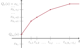
Figure 3: The map $[0,\infty)\to\operatorname{\mathbb{R}}$, $t\mapsto[g(t)](s)$ for a $s\in(0,1)$ with $Q_{\mu}(s)<Q_{\nu}(s)$ (left) and $Q_{\mu}(s)>Q_{\nu}(s)$ (right). The slopes of the affine linear pieces, determined by $s-R_{s,j}$, decrease for increasing $t$, that is, for increasing $j$.

Example 5.4.

Let

$$\mu_{0}\coloneqq\tfrac{1}{3}\delta_{-1}+\tfrac{1}{3}\delta_{1/2}+\tfrac{1}{3}\delta_{2}\quad\text{and}\quad\nu\coloneqq\tfrac{1}{4}\delta_{0}+\tfrac{3}{4}\delta_{1}.$$

The evolution of the quantile function can be computed as

$$[g(t)](s)=\begin{cases}\min\{2st-1,0\},&s\in(0,\frac{1}{4}),\\ \eqref{eq:excl-int},&s\in(\frac{1}{4},\frac{1}{3}),\\ \min\{(\frac{1}{2}-\frac{t}{4})+2st,1\},&s\in(\frac{1}{3},\frac{2}{3}),\\ \max\{(2-2t)-2st,1\}&s\in(\frac{2}{3},1),\end{cases}$$ (47)

where

$$[g(t)]\big{|}_{(\frac{1}{4},\frac{1}{3})}(s)=\begin{cases}2st-1,&s\leq t_{1}^{-1}(t),\\ \frac{1}{4s}-(\frac{t}{2}+1)+2st,&t_{1}^{-1}(t)\leq s\leq t_{2}^{-1}(t),\\ 1,&t_{2}^{-1}(t)\leq s\end{cases}$$ (48)

with the monotonically decreasing, continuous functions $t_{1}(s)\coloneqq t_{s,1}$ and $t_{2}(s)\coloneqq t_{s,2}$. Except for $s\in(1/4,1/3)$, the quantile function is piecewise linear, which corresponds to uniform measures and point measures. For $s\in(1/4,1/3)$, it becomes non-linear. The flow $g(t)_{\#}\Lambda_{(0,1)}$ is illustrated in Figure 4.

Figure 4: The Wasserstein gradient flow between the point measures in Example 5.4. The gray regions illustrate the density of the absolute continuous part of the flow, whereas the red spikes illustrate the discrete part. In the lower row, the mass from $\delta_{-1}$ split up, and a portion moves towards $\delta_{1}$. The movement speed of this portion, however, significantly decreases due to its attraction by $\delta_{0}$. Figuratively, the mass sticks to $\delta_{0}$ and can escape only slowly. For the corresponding densities see Figure 14.

6 Invariant Subsets and Smoothing Properties of $F_{\nu}$-Flows

In this section, we are interested in invariant subsets of $\operatorname{\mathcal{C}}(0,1)$, i.e., subsets in which $F_{\nu}$-flows remain once starting there. We also prove a smoothing result, where the $F_{\nu}$-flow immediately becomes more regular than the initial datum.

Note that [9, p. 131, Prop. 4.5] generally characterizes conditions for closed subsets to be invariant. However, we take a more refined approach involving the resolvent $J_{\varepsilon}^{\partial F_{\nu}}$, the exponential formula (17), and our explicit calculation (31) of $\partial F_{\nu}$. This approach will yield more precise results – and is not limited to closed subsets.

As a starting point, recall that $J_{\varepsilon}^{\partial F_{\nu}}$ maps $\operatorname{\mathcal{C}}(0,1)$ into itself by Lemma 4.4. By (31) this means: For all $\varepsilon>0$ and any $h\in\operatorname{\mathcal{C}}(0,1)$, there exists $u\in\operatorname{\mathcal{C}}(0,1)$ such that

$$u(s)+\varepsilon[R_{\nu}^{-}(u(s)),R_{\nu}^{+}(u(s))]~{}\ni~{}h(s)+\varepsilon s\hskip 8.53581pt\text{for a.e. }s\in(0,1).$$ (49)

To simplify the following arguments and notations, we identify an (equivalence class) $v\in\operatorname{\mathcal{C}}(0,1)$ with its unique left-continuous and increasing version, i.e. $v\coloneqq Q_{\mu_{v}}$, where $\mu_{v}\coloneqq v_{\#}\Lambda_{(0,1)}$, such that $v$ is uniquely defined everywhere on $(0,1)$ (and not only up to a null set) .

With the above identification of $v\in\operatorname{\mathcal{C}}(0,1)$ with its quantile function, the following lemma shows that (49) holds everywhere on $(0,1)$.

Lemma 6.1.

Let $\nu\in\operatorname{\mathcal{P}}_{2}(\operatorname{\mathbb{R}})$ be arbitrary. Then, for any $h\in\operatorname{\mathcal{C}}(0,1)$ there exists $u\coloneqq J_{\varepsilon/2}^{\partial F_{\nu}}h\in\operatorname{\mathcal{C}}(0,1)$ such that

$$u(s)+\varepsilon[R_{\nu}^{-}(u(s)),R_{\nu}^{+}(u(s))]~{}\ni~{}h(s)+\varepsilon s\hskip 8.53581pt\text{ for all }\hskip 8.53581pts\in(0,1).$$ (50)

The proof is given in the appendix.

Now, let $-\infty\leq a\leq b\leq\infty$ and $L>0$. We will study the following closed subsets of $\mathcal{C}(0,1)$:

1. bounded quantile functions:

   $$D_{[a,b]} :=\{Q_{\mu}\in\operatorname{\mathcal{C}}(0,1):\overline{Q_{\mu}(0,1)}\subseteq[a,b]\}=\{Q_{\mu}\in\operatorname{\mathcal{C}}(0,1):\operatorname{supp}\mu\subseteq[a,b]\},$$

2. quantile functions admitting a lower $L$-Lipschitz condition:

   $$D_{L}^{-} :=\{Q_{\mu}\in\operatorname{\mathcal{C}}(0,1):L\leq\frac{Q_{\mu}(s_{1})-Q_{\mu}(s_{2})}{s_{1}-s_{2}}~{}\text{ for all }s_{1},s_{2}\in(0,1)\},$$

3. $L$-Lipschitz continuous quantile functions:

   $$D_{L}^{+} :=\{Q_{\mu}\in\operatorname{\mathcal{C}}(0,1):\frac{Q_{\mu}(s_{1})-Q_{\mu}(s_{2})}{s_{1}-s_{2}}\leq L~{}\text{ for all }s_{1},s_{2}\in(0,1)\}.$$

We will also consider the following subset which is not closed in $\operatorname{\mathcal{C}}(0,1)$:

1. continuous quantile functions:

   $$D_{c} :=\{Q_{\mu}\in\operatorname{\mathcal{C}}(0,1):Q_{\mu}\text{ is continuous}\}$$

   $$=\{Q_{\mu}\in\operatorname{\mathcal{C}}(0,1):R_{\mu}^{+}\text{ is strictly increasing on }\overline{(R_{\mu}^{+})^{-1}(0,1)}\}$$

   $$=\{Q_{\mu}\in\operatorname{\mathcal{C}}(0,1):\operatorname{supp}\mu\text{ is convex}\}.$$

Note that the subset of quantile functions of absolutely continuous measures with respect to the Lebesgue measure is also not closed in $\mathcal{C}(0,1)$.

Next, we provide some examples of probability measures $\nu\in\operatorname{\mathcal{P}}_{2}(\operatorname{\mathbb{R}})$ and discuss to which of the sets from above their quantile functions belong.

Example 6.2.

1. For any atomic measure $\nu$ with a finite number of atoms we have $Q_{\nu}\in D_{[a,b]}$ for some $a,b\in\operatorname{\mathbb{R}}$ and $Q_{\nu}\not\in D_{L}^{-}$ for any $L>0$.

2. If $\nu$ defines a uniform distribution on $[a,b]$, then its quantile function is $s\mapsto a+s(b-a)$. Hence $Q_{\nu}\in D_{b-a}^{+}\cap D_{b-a}^{-}\cap D_{[a,b]}\cap D_{c}$.

3. For the normal distribution $\nu\sim\mathcal{N}(\mu,\sigma^{2})$, we have $\operatorname{supp}\nu=\operatorname{\mathbb{R}}$, so $Q_{\nu}\in D_{c}$, and that $Q_{\nu}(s)=\mu+\sqrt{2}\sigma\operatorname{erf}^{-1}(2s-1)$ is not Lipschitz continuous. However, $Q_{\nu}\in D_{L}^{-}$ with $L\coloneqq(2\pi\sigma^{2})^{\frac{1}{2}}$. The same is true for the Laplace distribution or a mixture of two normal distributions.

4. The exponential, Pareto and folded norm distributions, see (73), have a support that is unbounded in only one direction, so their quantile functions belong to $D_{c}\cap D_{[a,\infty)}$ for some $a\in\operatorname{\mathbb{R}}$. As above, these quantile functions do not belong to $D_{L}^{+}$, but to $D_{L}^{-}$.

Note that if $\mu\in\operatorname{\mathcal{P}}_{2}(\operatorname{\mathbb{R}})$ is absolutely continuous and $Q_{\mu}\not\in D_{[a,b]}$ for any $a,b\in\operatorname{\mathbb{R}}$, then we can not have $Q_{\mu}\in D_{L}^{+}$ for any $L>0$.

By the following Proposition 6.3, the above sets $D^{\pm}_{L}$ can be described in terms of CDFs instead of quantile functions, see Figure 5.

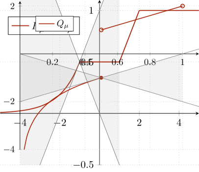
Figure 5: Left: $R_{\mu}^{+}$ is $\frac{1}{2}$-Lipschitz continuous, since there is a “double cone” (white) with extremal rays of slope $\frac{1}{2}$ such that if it is centered at any point of the graph of $R_{\mu}^{+}$, then the graph has no points within this double cone. Right: $Q_{\mu}$ admits a lower $2$-Lipschitz condition, since the white double cone with extremal rays of slope $2$ contains the whole graph of $Q_{\mu}$.

Proposition 6.3.

Let $Q_{\mu}\in\operatorname{\mathcal{C}}(0,1)$. Then the following holds true:

• $Q_{\mu}\in D_{L}^{-}$ if and only if $R_{\mu}=R_{\mu}^{+}$ is $\frac{1}{L}$-Lipschitz continuous, i.e.,

  $$\frac{R_{\mu}(x)-R_{\mu}(y)}{x-y}\leq\frac{1}{L}\quad\text{ for all }x,y\in\operatorname{\mathbb{R}}.$$ (51)

  In this case, $\mu$ is absolutely continuous, and the above holds iff its density $f_{\mu}$ fulfills

  $$f_{\mu}\leq\frac{1}{L}\quad\text{a.e. on }\operatorname{\mathbb{R}}.$$

• $Q_{\mu}\in D_{L}^{+}$ if and only if $R_{\mu}^{+}$ admits a lower $\frac{1}{L}$-Lipschitz condition on $\overline{(R_{\mu}^{+})^{-1}(0,1)}$, i.e.,

  $$\frac{1}{L}\leq\frac{R_{\mu}^{+}(x)-R_{\mu}^{+}(y)}{x-y}\quad\text{ for all }x,y\in\overline{(R_{\mu}^{+})^{-1}(0,1)}.$$ (52)

  If $\mu$ is absolutely continuous, then the above holds iff its density $f_{\mu}$ fulfills

  $$\frac{1}{L}\leq f_{\mu}\quad\text{a.e. on }\operatorname{conv}(\operatorname{supp}\mu).$$

The proof is given in the appendix.

The following proposition says that the support of flows cannot escape the convex hull of the support of the target measure $\nu$ once they start there.

Proposition 6.4 (Invariance of $D_{[a,b]}$).

Let $\nu\in\operatorname{\mathcal{P}}_{2}(\operatorname{\mathbb{R}})$ be such that $\overline{\operatorname{conv}}(\operatorname{supp}\nu)\subseteq[a,b]$. Then, $J_{\varepsilon}^{\partial F_{\nu}}$ maps $D_{[a,b]}$ into itself for all $\varepsilon>0$. Hence, the solution of the Cauchy problem (39) starting in $g_{0}\in D_{[a,b]}$ fulfills $g(t)\in D_{[a,b]}$ for all $t\geq 0$.

Proof.

Let $h\in D_{[a,b]}$ and consider a solution $u\in\operatorname{\mathcal{C}}(0,1)$ of (50). W.l.o.g., let $a,b$ be finite (otherwise there is nothing to show). Assume there exists $s^{*}\in(0,1)$ such that

$$u(s^{*})<a\leq\min(\operatorname{supp}\nu).$$

Then, it holds $R_{\nu}^{-}(u(s^{*}))=R_{\nu}^{+}(u(s^{*}))=0$ and by (50) that

$$a>u(s^{*})=h(s^{*})+\varepsilon s^{*}\geq a+\varepsilon s^{*},$$

which is a contradiction. Now, assume there is $s^{*}\in(0,1)$ such that

$$u(s^{*})>b\geq\max(\operatorname{supp}\nu).$$

Then, we obtain $R_{\nu}^{-}(u(s^{*}))=R_{\nu}^{+}(u(s^{*}))=1$ and by (50) further

$$b<u(s^{*})=h(s^{*})+\varepsilon(s^{*}-1)\leq b+\varepsilon(s^{*}-1),$$

again a contradiction. Together, we have proved $u(s)\in[a,b]$ for every $s\in(0,1)$, which shows $u\in D_{[a,b]}$. The remaining claim follows by Corollary 3.6. ∎

In order to prove invariance results for $D_{L}^{-}$ and $D_{L}^{+}$, we define for given $Q_{\mu}\in\operatorname{\mathcal{C}}(0,1)$ the largest lower Lipschitz constant

$$L_{\text{low}}(Q_{\mu}):=\max\{L\geq 0:\frac{Q_{\mu}(s_{1})-Q_{\mu}(s_{2})}{s_{1}-s_{2}}\geq L~{}\text{ for all }s_{1},s_{2}\in(0,1)\}\geq 0,$$

where $L_{\text{low}}(Q_{\mu})=0$ is explicitly allowed. Note that by Proposition 6.3, it holds $L_{\text{low}}(Q_{\mu})>0$ if and only if $R_{\mu}$ is Lipschitz continuous with constant $L_{\text{low}}(Q_{\mu})^{-1}$. Further, consider the usual smallest Lipschitz constant

$${\rm Lip}(Q_{\mu}):=\min\{L\geq 0:\frac{Q_{\mu}(s_{1})-Q_{\mu}(s_{2})}{s_{1}-s_{2}}\leq L~{}\text{ for all }s_{1},s_{2}\in(0,1)\}\leq\infty.$$

By Proposition 6.3, it holds $0<{\rm Lip}(Q_{\mu})<\infty$ if and only if $R_{\mu}^{+}$ admits a lower ${\rm Lip}(Q_{\mu})^{-1}$-Lipschitz condition on $\overline{(R_{\mu}^{+})^{-1}(0,1)}$.

Now, we can formulate an invariance and smoothing property of $F_{\nu}$-flows. In addition, we can accurately describe how the Lipschitz constants of the $F_{\nu}$-flow evolve over time. We start with the lower constant.

Theorem 6.5.

Let $\nu\in\operatorname{\mathcal{P}}_{2}(\operatorname{\mathbb{R}})$ with $L_{{\rm low}}(Q_{\nu})>0$. Consider any initial value $g_{0}=Q_{\mu_{0}}\in\operatorname{\mathcal{C}}(0,1)$, where $L_{{\rm low}}(g_{0})=0$ is explicitly allowed. Then, the strong solution $g:[0,\infty)\to\operatorname{\mathcal{C}}(0,1)$ of the Cauchy problem (39) enjoys for all $t>0$ the smoothing property

$$L_{{\rm low}}(g(t))\geq L_{{\rm low}}(g_{0})\cdot e^{-\frac{2t}{L_{{\rm low}}(Q_{\nu})}}+L_{{\rm low}}(Q_{\nu})\cdot(1-e^{-\frac{2t}{L_{{\rm low}}(Q_{\nu})}})>0.$$ (53)

In particular, the CDF $R_{\gamma_{t}}$ of the associated Wasserstein gradient flow $\gamma_{t}$ is Lipschitz continuous for any $t>0$ with Lipschitz constant

$${\rm Lip}(R_{\gamma_{t}})\leq\Big{(}L_{{\rm low}}(g_{0})\cdot e^{-\frac{2t}{L_{{\rm low}}(Q_{\nu})}}+L_{{\rm low}}(Q_{\nu})\cdot(1-e^{-\frac{2t}{L_{{\rm low}}(Q_{\nu})}})\Big{)}^{-1}<\infty.$$ (54)

Proof.

i) First, let $h\in\operatorname{\mathcal{C}}(0,1)$ and $\varepsilon>0$. By (50) and since $R_{\nu}^{+}=R_{\nu}^{-}=R_{\nu}$ is continuous, there exists a solution $u\in\operatorname{\mathcal{C}}(0,1)$ of

$$h(s)+\varepsilon s=u(s)+\varepsilon R_{\nu}(u(s))\quad\text{for all }s\in(0,1).$$

By the Lipschitz continuity of $R_{\nu}$, it holds for all $s_{1},s_{2}\in(0,1)$, $s_{1}>s_{2}$, that

$$\frac{u(s_{1})-u(s_{2})}{s_{1}-s_{2}} =\frac{h(s_{1})-h(s_{2})}{s_{1}-s_{2}}+\varepsilon-\varepsilon\frac{R_{\nu}(u(s_{1}))-R_{\nu}(u(s_{2}))}{s_{1}-s_{2}}$$

$$\geq L_{\text{low}}(h)+\varepsilon-\varepsilon\frac{1}{L_{\text{low}}(Q_{\nu})}\cdot\frac{u(s_{1})-u(s_{2})}{s_{1}-s_{2}},$$

which yields

$$\frac{u(s_{1})-u(s_{2})}{s_{1}-s_{2}}\geq\frac{L_{\text{low}}(h)+\varepsilon}{q},\quad q\coloneqq 1+\frac{\varepsilon}{L_{\text{low}}(Q_{\nu})}.$$

This means $L_{\text{low}}(u)\geq\frac{L_{\text{low}}(h)+\varepsilon}{q}>0$. (Notice the improvement $L_{\text{low}}(u)>0$, even if $L_{\text{low}}(h)=0$.) We have proved for any $h\in\operatorname{\mathcal{C}}(0,1)$ and any $\varepsilon>0$ that

$$L_{\text{low}}((I+\frac{\varepsilon}{2}\partial F_{\nu})^{-1}h)\geq\frac{L_{\text{low}}(h)+\varepsilon}{q}.$$ (55)

Now, fix $n\in\operatorname{\mathbb{N}}$ and observe inductively that

$$L_{\text{low}}((I+\frac{\varepsilon}{2}\partial F_{\nu})^{-n}g_{0}) \geq\frac{L_{\text{low}}((I+\frac{\varepsilon}{2}\partial F_{\nu})^{-(n-1)}g_{0})}{q}+\frac{\varepsilon}{q}$$

$$\geq\frac{L_{\text{low}}((I+\frac{\varepsilon}{2}\partial F_{\nu})^{-(n-2)}g_{0})}{q^{2}}+\frac{\varepsilon}{q^{2}}+\frac{\varepsilon}{q}\geq\ldots$$

$$\geq\frac{L_{\text{low}}(g_{0})}{q^{n}}+\varepsilon\sum_{k=1}^{n}\frac{1}{q^{k}}$$

$$=\frac{L_{\text{low}}(g_{0})}{q^{n}}+\frac{\varepsilon}{q}\cdot\frac{1-q^{-n}}{1-q^{-1}}$$

$$=\frac{L_{\text{low}}(g_{0})}{q^{n}}+L_{\text{low}}(Q_{\nu})(1-q^{-n}).$$

Now, for $t>0$ and choosing $\varepsilon\coloneqq\frac{2t}{n}$, it follows

$$L_{\text{low}}((I+\frac{t}{n}\partial F_{\nu})^{-n}g_{0}) \geq\frac{L_{\text{low}}(g_{0})}{(1+\frac{2t}{nL_{\text{low}}(Q_{\nu})})^{n}}+L_{\text{low}}(Q_{\nu})(1-(1+\frac{2t}{nL_{\text{low}}(Q_{\nu})})^{-n})$$

$$\overset{n\uparrow\infty}{\longrightarrow}L_{\text{low}}(g_{0})\cdot e^{-\frac{2t}{L_{\text{low}}(Q_{\nu})}}+L_{\text{low}}(Q_{\nu})\cdot(1-e^{-\frac{2t}{L_{\text{low}}(Q_{\nu})}}).$$

Finally, the solution $g:[0,\infty)\to\operatorname{\mathcal{C}}(0,1)$ of the Cauchy problem (39) is given by the exponential formula (and $L_{2}$-limit) (17) which implies

$$L_{\text{low}}(g(t))\geq L_{\text{low}}(g_{0})\cdot e^{-\frac{2t}{L_{\text{low}}(Q_{\nu})}}+L_{\text{low}}(Q_{\nu})\cdot(1-e^{-\frac{2t}{L_{\text{low}}(Q_{\nu})}})>0$$ (56)

for all $t>0$, which concludes the proof. ∎

Note that even if the initial measure satisfies $L_{{\rm low}}(g_{0})=0$ (e.g., atomic measures), the Lipschitz continuity of the target CDF, i.e., $L_{{\rm low}}(Q_{\nu})>0$, is enough to force the flow’s CDFs to immediately become Lipschitz continuous for any $t>0$, and the Lipschitz constants exponentially improve for $t\to\infty$ towards the target Lipschitz constant $L_{{\rm low}}(Q_{\nu})^{-1}$ as described in (54).

The following example demonstrates that the bound (54) of the Lipschitz constants in Theorem 6.5 is sharp.

Example 6.6.

Consider as target measure $\nu$ the uniform distribution on $[0,1]$, and as initial measure $\mu_{0}\coloneqq\delta_{0}$ the Dirac measure at $0$. Then, for the corresponding CDFs, we get that

$$R_{\nu}(x)=\begin{cases}0,&~{}x\leq 0,\\ x,&~{}0<x<1,\\ 1,&~{}x\geq 1\end{cases}$$ (57)

is $1$-Lipschitz continuous, whereas

$$R_{\mu_{0}}^{+}(x)=\begin{cases}0,&~{}x<0,\\ 1,&~{}x\geq 0.\end{cases}$$ (58)

is a jump function. Still, the $\operatorname{\mathcal{F}}_{\nu}$-Wasserstein gradient flow $\gamma_{t}$ immediately regularizes to uniform distributions for $t>0$ given by

$$R_{\gamma_{t}}(x)=\begin{cases}0,&~{}x\leq 0,\\ (1-e^{-2t})^{-1}x,&~{}0<x<1-e^{-2t},\\ 1,&~{}x\geq 1-e^{-2t},\end{cases}$$ (59)

which are $(1-e^{-2t})^{-1}$-Lipschitz continuous. Thus, the upper bound of the Lipschitz constants (54) is sharp.

Next, we deal with the upper Lipschitz constant.

Theorem 6.7.

Let $\nu\in\operatorname{\mathcal{P}}_{2}(\operatorname{\mathbb{R}})$ such that $\operatorname{supp}\nu=[a,b]$ and ${\rm Lip}(Q_{\nu})<\infty$. Consider an initial value $g_{0}=Q_{\mu_{0}}\in\operatorname{\mathcal{C}}(0,1)$ with convex support $\operatorname{supp}{\mu_{0}}\subseteq[a,b]$ and ${\rm Lip}(g_{0})<\infty$. Then, the strong solution $g:[0,\infty)\to\operatorname{\mathcal{C}}(0,1)$ of the Cauchy problem (39) fulfills for all $t>0$ the invariance property

$${\rm Lip}(g(t))\leq{\rm Lip}(g_{0})\cdot e^{-\frac{2t}{{\rm Lip}(Q_{\nu})}}+{\rm Lip}(Q_{\nu})\cdot(1-e^{-\frac{2t}{{\rm Lip}(Q_{\nu})}})<\infty.$$ (60)

In particular, the CDF $R_{\gamma_{t}}^{+}$ of the associated Wasserstein gradient flow $\gamma_{t}$ admits a lower Lipschitz constant on $\overline{(R_{\gamma_{t}}^{+})^{-1}(0,1)}$ for all $t>0$, and the constant is

$$L_{\rm low}(R_{\gamma_{t}}^{+})\geq\Big{(}{\rm Lip}(g_{0})\cdot e^{-\frac{2t}{{\rm Lip}(Q_{\nu})}}+{\rm Lip}(Q_{\nu})\cdot(1-e^{-\frac{2t}{{\rm Lip}(Q_{\nu})}})\Big{)}^{-1}>0.$$ (61)

Proof.

If ${\rm Lip}(Q_{\nu})=0$, then by assumption, it holds $\operatorname{supp}{\mu_{0}}\subseteq\operatorname{supp}{\nu}=\{a\}$. Hence, the solution of (39) is given by $g(t)\equiv a$ for all $t\geq 0$, and trivially satisfies (60). So, we can assume that ${\rm Lip}(Q_{\nu})>0$. Now, let $h\in D_{[a,b]}$ with ${\rm Lip}(h)<\infty$, and $\varepsilon>0$. By Proposition 6.4, there exists a solution $u\in D_{[a,b]}$ of (50). Let $s_{1},s_{2}\in(0,1)$, $s_{1}>s_{2}$. W.l.o.g., we can assume that $u(s_{2})<u(s_{1})$. Hence, we can choose $\kappa>0$ small enough such that $a\leq u(s_{2})<u(s_{1})-\kappa\leq b$. Now, by (50), it holds

$$u(s_{1})\leq h(s_{1})+\varepsilon s_{1}-\varepsilon R_{\nu}^{-}(u(s_{1}))$$ (62)

and

$$u(s_{2})\geq h(s_{2})+\varepsilon s_{2}-\varepsilon R_{\nu}^{+}(u(s_{2})).$$ (63)

By Proposition 6.3, $R_{\nu}^{+}$ admits a lower ${\rm Lip}(Q_{\nu})^{-1}$-Lipschitz condition on
$\overline{(R_{\nu}^{+})^{-1}(0,1)}=\operatorname{supp}\nu=[a,b]$, so that

$$\frac{u(s_{1})-u(s_{2})}{s_{1}-s_{2}} \leq\frac{h(s_{1})-h(s_{2})}{s_{1}-s_{2}}+\varepsilon-\varepsilon\frac{R_{\nu}^{-}(u(s_{1}))-R_{\nu}^{+}(u(s_{2}))}{s_{1}-s_{2}}$$

$$\leq\frac{h(s_{1})-h(s_{2})}{s_{1}-s_{2}}+\varepsilon-\varepsilon\frac{R_{\nu}^{+}(u(s_{1})-\kappa)-R_{\nu}^{+}(u(s_{2}))}{s_{1}-s_{2}}$$

$$\leq\frac{h(s_{1})-h(s_{2})}{s_{1}-s_{2}}+\varepsilon-\varepsilon\frac{1}{{\rm Lip}(Q_{\nu})}\cdot\frac{(u(s_{1})-\kappa)-u(s_{2})}{s_{1}-s_{2}}.$$

Letting $\kappa\downarrow 0$ leads to

$$\frac{u(s_{1})-u(s_{2})}{s_{1}-s_{2}}\leq{\rm Lip}(h)+\varepsilon-\frac{\varepsilon}{{\rm Lip}(Q_{\nu})}\cdot\frac{u(s_{1})-u(s_{2})}{s_{1}-s_{2}},$$

which yields

$$\frac{u(s_{1})-u(s_{2})}{s_{1}-s_{2}}\leq\frac{{\rm Lip}(h)+\varepsilon}{q},\quad q\coloneqq 1+\frac{\varepsilon}{{\rm Lip}(Q_{\nu})}.$$

This shows ${\rm Lip}(u)\leq\frac{{\rm Lip}(h)+\varepsilon}{q}<\infty$. In other words, for any $h\in D_{[a,b]}$ with ${\rm Lip}(h)<\infty$ and $\varepsilon>0$, it holds

$${\rm Lip}((I+\frac{\varepsilon}{2}\partial F_{\nu})^{-1}h)\leq\frac{{\rm Lip}(h)+\varepsilon}{q}.$$ (64)

Now, setting $h:=g_{0}$, we obtain the desired estimate (60) in the same lines as in the previous proof, and we are done. ∎

We mention that formally, the conditions ${\rm Lip}(Q_{\nu})<\infty$ and ${\rm Lip}(Q_{\mu_{0}})=\infty$ bring no improvement in the estimate (60) for ${\rm Lip}(g(t))$. Further, by the following example, the support assumption in Theorem 6.7 cannot be skipped.

Example 6.8.

In our example in the introduction, we considered the Wasserstein gradient flow from $\mu_{0}=\delta_{-1}$ to $\nu=\delta_{0}$ with ${\rm Lip}(Q_{\mu_{0}})={\rm Lip}(Q_{\nu})=0$. By Corollary 5.3, the quantile functions given by

$$[g(t)](s)=\min\{2st-1,0\}.$$ (65)

are piecewise linear and sharply contained in $D_{2t}^{+}$, see Figure 6. In particular, the Lipschitz constants cannot be bounded. The corresponding Wasserstein gradient flow reads as

$$\gamma_{t}=\begin{cases}\delta_{-1},&t=0,\\ \tfrac{1}{2t}\Lambda_{[-1,-1+2t]},&0\leq t\leq\frac{1}{2},\\ \tfrac{1}{2t}\Lambda_{[-1,0]}+\bigl{(}1-\tfrac{1}{2t}\bigr{)}\delta_{0},&\frac{1}{2}<t,\end{cases}$$ (66)

and was already depicted in Figure 1.

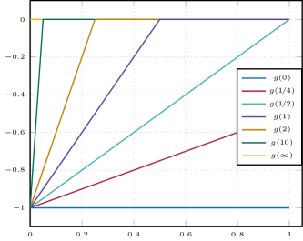
Figure 6: The functions $g(t)$ from (65) for $t\in\{0,\frac{1}{4},\frac{1}{2},1,2,10\}$.

As a consequence of Theorems 6.5, 6.7 and their proofs, we immediately obtain the following invariance properties of $D_{L}^{-}$ and $D_{[a,b]}\cap D_{L}^{+}$ with respect to the $F_{\nu}$-flow.

Corollary 6.9 (Invariance of $D_{L}^{-}$ and $D_{L}^{+}\cap D_{[a,b]}$).

Let $\nu\in\operatorname{\mathcal{P}}_{2}(\operatorname{\mathbb{R}})$.

1. Assume $Q_{\nu}\in D_{L}^{-}$. Then, the solution of the Cauchy problem (39) starting in $g_{0}\in D_{L}^{-}$ fulfills $g(t)\in D_{L}^{-}$ for all $t\geq 0$. More precisely, it holds (53). Moreover, $J_{\varepsilon}^{\partial F_{\nu}}$ maps $D_{L}^{-}$ into itself for all $\varepsilon>0$.

   In particular, if the initial measure $\mu_{0}$ has a $L_{0}$-Lipschitz continuous CDF $R_{\mu_{0}}$, then the flow’s CDF $R_{\gamma_{t}}$ remains Lipschitz (and thus absolutely) continuous with constant $\leq\max\{L_{0},L^{-1}\}$ for all $t\geq 0$.

2. Assume $\operatorname{supp}\nu=[a,b]$ and $Q_{\nu}\in D_{L}^{+}$. Then, the solution of the Cauchy problem (39) starting in $g_{0}\in D_{[a,b]}\cap D_{L}^{+}$ fulfills $g(t)\in D_{[a,b]}\cap D_{L}^{+}$ for all $t\geq 0$. More precisely, it holds (60).
   Moreover, $J_{\varepsilon}^{\partial F_{\nu}}$ maps $D_{[a,b]}\cap D_{L}^{+}$ into itself for all $\varepsilon>0$.

   In particular, if the initial measure $\mu_{0}$ has convex support $\operatorname{supp}\mu_{0}\subseteq[a,b]$ and is in $D_{L}^{+}$, then $\gamma_{t}$ has convex support for all $t\geq 0$ and no ’gaps’ of empty mass can form.

Note that in part i), no point masses can arise during the flow – given that the target measure is Lipschitz continuous – as opposed to the example of Figure 1.

Finally, we study the set $D_{c}$ of continuous quantile functions. By the following lemma, it is also invariant with respect to the resolvent $J_{\varepsilon}^{\partial F_{\nu}}$.

Lemma 6.10.

Let $\nu\in\operatorname{\mathcal{P}}_{2}(\operatorname{\mathbb{R}})$ be arbitrary. Then, $J_{\varepsilon}^{\partial F_{\nu}}$ maps $D_{c}$ into itself for all $\varepsilon>0$.

Proof.

For $h\in D_{c}$, we consider a solution $u\in\operatorname{\mathcal{C}}(0,1)$ of (50). Suppose that $u$ is not continuous at some $s_{0}\in(0,1)$. Since $u$ is left-continuous and increasing, we have $\lim_{t\downarrow s_{0}}u(t)>u(s_{0})$. But then, (50) and the continuity of $h$ imply

$$h(s_{0})+\varepsilon s_{0} =\lim_{t\downarrow s_{0}}\left(h(t)+\varepsilon t\right)\geq\lim_{t\downarrow s_{0}}\left(u(t)+\varepsilon R_{\nu}^{-}(u(t))\right)$$

$$>u(s_{0})+\varepsilon R_{\nu}^{+}(u(s_{0}))\geq h(s_{0})+\varepsilon s_{0},$$

a contradiction. Thus, $u\in D_{c}$. ∎

Since $D_{c}$ is not closed with respect to the $L_{2}$-norm, Corollary 3.6 cannot be applied directly. Still, we have the following invariance and monotonicity result. Note that there are no restrictions on the target measure $\nu\in\operatorname{\mathcal{P}}_{2}(\operatorname{\mathbb{R}})$.

Theorem 6.11 (Invariance of $D_{c}$ & monotonicity of the support).

Let $\nu\in\operatorname{\mathcal{P}}_{2}(\operatorname{\mathbb{R}})$ and $g_{0}\in D_{c}$. Then the following holds true:

1. The solution $g$ of the Cauchy problem (39) starting in $g_{0}\in D_{c}$ fulfills $g(t)\in D_{c}$ for all $t\geq 0$.

2. The ranges fulfill $\overline{g(t_{1})(0,1)}\subseteq\overline{g(t_{2})(0,1)}$ for all $0\leq t_{1}\leq t_{2}$.

In other words the theorem says: if the initial measure $\mu_{0}$ has convex support, then $\operatorname{supp}\gamma_{t}$ stays convex for all $t\geq 0$, and we have the monotonicity $\operatorname{supp}\gamma_{t_{1}}\subseteq\operatorname{supp}\gamma_{t_{2}}$ for all $0\leq t_{1}\leq t_{2}$.

Proof.

i) Fix $t>0$. For the initial datum $g_{0}\in D_{c}$, Lemma 6.10 yields

$$g_{n}\coloneqq(I+\frac{t}{n}\partial F_{\nu})^{-n}g_{0}\in D_{c}\quad\text{ for all }n\in\operatorname{\mathbb{N}}.$$

We verify that $(g_{n})_{n\in\operatorname{\mathbb{N}}}$ fulfills the assumptions of the Arzelà-Ascoli theorem.
1) Fix $s\in(0,1)$ and $n\in\operatorname{\mathbb{N}}$. By (50), it holds for $u\coloneqq(I+\frac{t}{n}\partial F_{\nu})^{-1}g_{0}$ that

$$u(s) \leq g_{0}(s)+\frac{2t}{n}s-\frac{2t}{n}R_{\nu}^{-}(u(s))\leq g_{0}(s)+\frac{2t}{n}s,$$

$$u(s) \geq g_{0}(s)+\frac{2t}{n}s-\frac{2t}{n}R_{\nu}^{+}(u(s))\geq g_{0}(s)+\frac{2t}{n}s-\frac{2t}{n},$$

so that

$$|u(s)|\leq|g_{0}(s)|+\frac{2t}{n}(s+1).$$

Iteratively, it follows

$$|g_{n}(s)|\leq|g_{0}(s)|+2t(s+1).$$

Since $n\in\operatorname{\mathbb{N}}$ was arbitrary, $(g_{n})_{n}$ is pointwise bounded.
2) Fix $0<s_{2}<s_{1}<1$ and $n\in\operatorname{\mathbb{N}}$. W.l.o.g. we can assume for $u$ as above that $u(s_{2})<u(s_{1})$. Since $R_{\nu}^{-}(u(s_{1}))-R_{\nu}^{+}(u(s_{2}))\geq 0$, it follows by (50) that

$$|u(s_{1})-u(s_{2})| \leq g_{0}(s_{1})-g_{0}(s_{2})+\frac{2t}{n}(s_{1}-s_{2})-\frac{2t}{n}\big{(}R_{\nu}^{-}(u(s_{1}))-R_{\nu}^{+}(u(s_{2}))\big{)}$$

$$\leq|g_{0}(s_{1})-g_{0}(s_{2})|+\frac{2t}{n}|s_{1}-s_{2}|.$$

Again, it follows inductively that

$$|g_{n}(s_{1})-g_{n}(s_{2})|\leq|g_{0}(s_{1})-g_{0}(s_{2})|+2t|s_{1}-s_{2}|.$$

Since $n\in\operatorname{\mathbb{N}}$ was arbitrary, $(g_{n})_{n\in\operatorname{\mathbb{N}}}$ is equicontinuous.
Now let $K\subset(0,1)$ be compact. By Arzelà-Ascoli’s theorem, (for a subsequence) $(g_{n})$ converges uniformly on $K$ to a continuous function $\tilde{g}\colon K\to\operatorname{\mathbb{R}}$. By the exponential formula (17), the $L_{2}$-limit of $(g_{n})$ is already given by $g(t)$. By the uniqueness of the limit, it follows that $g(t)|_{K}\equiv\tilde{g}$ is continuous on $K$. Since $K$ was an arbitrary compact subset of $(0,1)$, we obtain that $g(t)$ is continuous on $(0,1)$, which means $g(t)\in D_{c}$ as claimed.
ii) For the monotonicity claim, let $0\leq t_{1}\leq t_{2}<\infty$ be arbitrary fixed. The strong solution $g$ of the Cauchy problem (39) has the Bochner integral representation

$$g(t_{2})=\int_{t_{1}}^{t_{2}}\partial_{t}g(t)\mathop{}\!\mathrm{d}t+g(t_{1}),$$

which allows a pointwise evaluation

$$g(t_{2})(s)=\int_{t_{1}}^{t_{2}}\partial_{t}g(t)(s)\mathop{}\!\mathrm{d}t+g(t_{1})(s)\quad\text{for a.e. }s\in(0,1).$$

Since $\partial_{t}g(t)\in-\partial F_{\nu}(g(t))$ for a.e. $t>0$, and noting that $0\leq R_{\nu}^{-}\leq R_{\nu}^{+}\leq 1$, it follows for a.e. $s\in(0,1)$ that

$$g(t_{2})(s) \leq\int_{t_{1}}^{t_{2}}2s-2R_{\nu}^{-}\big{(}g(t)(s)\big{)}\mathop{}\!\mathrm{d}t+g(t_{1})(s)$$

$$\leq 2s(t_{2}-t_{1})+g(t_{1})(s).$$

This yields

$$\lim_{s\downarrow 0}g(t_{2})(s)\leq\lim_{s\downarrow 0}g(t_{1})(s).$$ (67)

Analogously, it holds for a.e. $s\in(0,1)$ that

$$g(t_{2})(s) \geq\int_{t_{1}}^{t_{2}}\Big{(}2s-2R_{\nu}^{+}\big{(}g(t)(s)\big{)}\Big{)}\mathop{}\!\mathrm{d}t+g(t_{1})(s)$$

$$\geq 2(s-1)(t_{2}-t_{1})+g(t_{1})(s),$$

which implies

$$\lim_{s\uparrow 1}g(t_{2})(s)\geq\lim_{s\uparrow 1}g(t_{1})(s).$$ (68)

Combining (67) and (68), we have proved that

$$\lim_{s\downarrow 0}g(t_{2})(s)\leq\lim_{s\downarrow 0}g(t_{1})(s)\leq\lim_{s\uparrow 1}g(t_{1})(s)\leq\lim_{s\uparrow 1}g(t_{2})(s).$$ (69)

By part i), we know that $g(t_{2})\in D_{c}$. The intermediate value theorem finally implies that $\overline{g(t_{1})(0,1)}\subseteq\overline{g(t_{2})(0,1)}$, and we are done. ∎

Remark 6.12.

Theorem 6.11 states that the support of the flow $\gamma_{t}$ monotonically increases with the time $t$, given that the initial support $\operatorname{supp}\mu_{0}$ is convex. We leave it as an open problem, whether this still holds in general without the convexity assumption on $\operatorname{supp}\mu_{0}$.

In Appendix A.4, we highlight some statements of this section from a different point of view.

7 Numerical Experiments

In this section, we first discuss a backward and a forward Euler scheme for the numerical computation of the one-dimensional MMD flow with the negative distance kernel and give some examples afterwards.

7.1 Euler Schemes

Implicit (backward) Euler scheme.

The minimizing movement scheme (9), see also JKO scheme [28],

$$\mu_{n+1}\coloneqq\operatorname*{arg\,min}_{\mu\in\operatorname{\mathcal{P}}_{2}(\operatorname{\mathbb{R}}^{d})}\Big{\{}\operatorname{\mathcal{F}}_{\nu}(\mu)+\frac{1}{2\tau}W_{2}^{2}(\mu_{n},\mu)\Big{\}},\qquad\tau>0,$$

can be rewritten by Theorem 3.2 in terms of quantile functions as

$$g_{n+1}=\operatorname*{arg\,min}_{g\in\mathcal{C}(0,1)}\Big{\{}F_{\nu}(g)+\frac{1}{2\tau}\int_{0}^{1}|g-g_{n}|^{2}\mathop{}\!\mathrm{d}s\Big{\}},\qquad\tau>0.$$ (70)

Because $F_{\nu}$ is proper, convex and lsc, the solution of this problem is given by (also see (17))

$$g_{n+1}=(I+\tau\partial F_{\nu})^{-1}(g_{n})$$ (71)

which is by Lemma 4.3 and Lemma 6.1 equivalent to

$$g_{n}(s)+2\tau s\in g_{n+1}(s)+2\tau[R_{\nu}^{-}(g_{n+1}(s)),R_{\nu}^{+}(g_{n+1}(s))]\qquad\text{for all }s\in(0,1).$$ (72)

Note that by Lemma 6.1 the functions $g_{n}$ and $g_{n+1}$ are quantile functions and thus increasing, so that $g_{n}+2\tau I$ is strictly increasing. Figure 7 gives a visual intuition for solving (72).

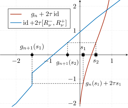
Figure 7: Implicit Euler step visualized for $g_{n}=Q_{\gamma_{n}}$ with $\gamma_{n}\sim\operatorname{\mathcal{N}}(0,1)$ and $\tau=\tfrac{1}{2}$ and $\nu$ being a mixture of two uniform distributions. Starting from any point $s_{1}\in(0,1)$ and $y\coloneqq(g_{n}+2\tau I)(s_{1})$, we are searching for $x\coloneqq g_{n+1}(s)\in\operatorname{\mathbb{R}}$ such that $y\in x+2\tau[R_{\nu}^{-}(x),R_{\nu}^{+}(x)]$. This is also illustrated for a point $s_{2}\in(0,1)$.

For fixed $\tau>0$, we perform $n=1,2,\ldots$ implicit Euler steps (71) via solving (72). By Theorem 2.1, we see that $(g_{n})_{\#}\Lambda_{(0,1)}$ can be considered as an approximation of the Wasserstein gradient flow in the time interval $(n\tau,(n+1)\tau]$. Further, for fixed $\tau$ and $n\to\infty$, the sequence $(g_{n})_{n\in\operatorname{\mathbb{N}}}$ converges weakly to $Q_{\nu}$ in $L_{2}(0,1)$, see [3, 34], and the corresponding measures $\mu_{n}\coloneqq(g_{n})_{\#}\Lambda_{(0,1)}$ converge narrowly to the minimizer $\nu$ of $\mathcal{F}_{\nu}$, see [32, Thm 6.7]. The scheme (71) resembles a proximal point algorithm, and for convergence results for more general so-called quasi $\alpha$-firmly nonexpansive mappings (instead of just proximal mappings), we refer to [5].

Explicit (forward) Euler scheme.

For constant step size $\tau>0$, we will also consider the explicit Euler discretization

$$g_{n+1}=g_{n}-\tau\nabla F_{\nu}(g_{n}),$$

which is only available if $R^{+}_{\nu}=R^{-}_{\nu}=:R_{\nu}$ is continuous, so that

$$\nabla F_{\nu}(g)=2R_{\nu}\circ g-2I,\qquad g\in L_{2}(0,1).$$

The explicit Euler scheme has the advantage that we do not have to solve an inclusion in each step. However, this method comes with weaker convergence guarantees. Moreover, it might not preserve $\operatorname{\mathcal{C}}(0,1)$, that is, the iterates might not be monotone. In all our numerical examples we chose $\tau=\tfrac{1}{100}$, which preserved monotonicity. However, monotonicity was not preserved for large step sizes, e.g., $\tau=2$.

7.2 Numerical Experiments

Next, we compare the implicit and explicit Euler schemes for various combinations of absolutely continuous initial and target measures. The following examples are covered by Theorem 6.5, or Corollary 6.9 i): since $L_{\text{low}}(Q_{\nu})>0$ in each figure, we have $L_{\text{low}}(Q_{\gamma_{t}})>0$ for all $t>0$.

Flow between two Gaussians, resp., Laplacians.

In Figure 8 we plot the MMD flow, where $\mu_{0}$ and $\nu$ are both Gaussians with different means, but equal variance. Although the qualitative behaviors of the implicit and explicit schemes are similar, the explicit scheme “is ahead of” the implicit one. In particular, we observe that the shape of the normal distribution is not at all preserved during the flow and that instead the densities first spread out and become more flat and then form a peak again, when they meet the mean of the target distribution.

In Figure 9, this behavior can also be observed when the initial and the target measure are both Laplacians. Here we can also see that the non-differentiability of the density at its peak is smoothed out and then re-created during the flow.

In Figure 10 we plot the MMD flow, where $\mu_{0}$ and $\nu$ are both Gaussians with different variance but equal mean. Again, the behavior of both discretizations is similar, just shifted in time, and the measures do not stay Gaussian. In particular, as predicted by Theorem 6.11 the visible support of $\gamma_{t}$ is strictly increasing and matches the tails of the target distribution only exponentially slowly.

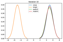
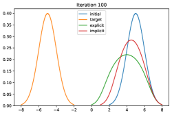
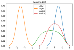
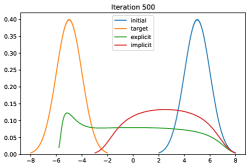
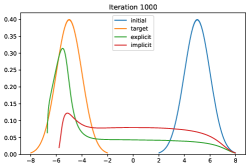
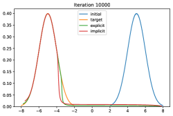
Figure 8: Comparison of implicit (red) and explicit (green) Euler schemes between two Gaussians $\mu_{0}\sim\operatorname{\mathcal{N}}(5,1)$ and $\nu\sim\operatorname{\mathcal{N}}(-5,1)$ with $\tau=\tfrac{1}{100}$. For the corresponding quantile functions, see Figure 15.

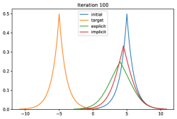
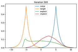
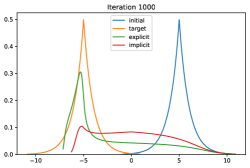
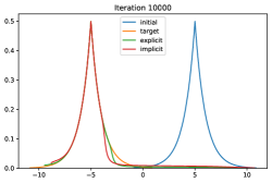
Figure 9: Comparison of implicit (red) and explicit (green) Euler schemes between two Laplacians $\mu_{0}\sim\mathcal{L}(5,1)$ and $\nu\sim\mathcal{L}(-5,1)$ with $\tau=\tfrac{1}{100}$. For the corresponding quantile functions, see Figure 16.

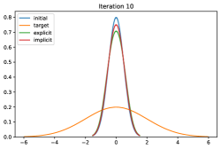
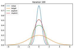
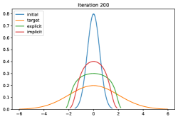
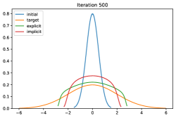
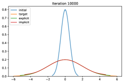
Figure 10: Comparison of implicit (red) and explicit (green) Euler schemes between two Gaussians $\mu_{0}\sim\operatorname{\mathcal{N}}(0,\sqrt{2})$ and $\nu\sim\operatorname{\mathcal{N}}(0,\tfrac{1}{\sqrt{2}})$ with $\tau=\tfrac{1}{100}$. For the corresponding quantile functions, see Figure 17.

Flow between measures with different number of modes.

Consider now the case where the initial measure $\mu_{0}$ is a Gaussian mixture model, which is symmetric with respect to the origin, and $\nu$ is a standard Gaussian. This case is plotted in Figure 11. We observe a similar relation between implicit and explicit scheme as in the previous example. Interestingly, we see that when the two parts of the visible support of $\gamma_{t}$ collide at the origin, it takes a lot of time to recover the peak of the target measure, that is, the region of high density is recovered after regions of lower density.

In Figure 12 we switch initial and target measure. Here, we observe a similar behavior as in Figure 8: first the densities spread out and become more flat, and the two peaks of the target are developed not until the density meets the modes of the target.

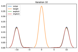
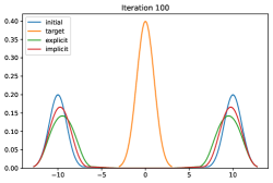
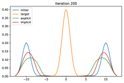
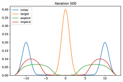
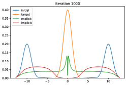
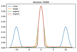
Figure 11: Comparison of implicit (red) and explicit (green) Euler schemes between $\mu_{0}\sim\frac{1}{2}\operatorname{\mathcal{N}}(-10,1)+\frac{1}{2}\operatorname{\mathcal{N}}(10,1)$ and $\nu\sim\operatorname{\mathcal{N}}(0,1)$ with $\tau=\tfrac{1}{100}$. For the corresponding quantile functions, see Figure 18.

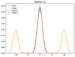
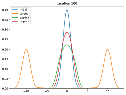
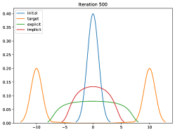
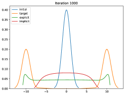
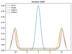
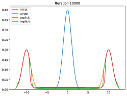
Figure 12: Comparison of implicit (red) and explicit (green) Euler schemes between $\mu_{0}\sim\operatorname{\mathcal{N}}(0,1)$ and $\nu\sim\frac{1}{2}\operatorname{\mathcal{N}}(-10,1)+\frac{1}{2}\operatorname{\mathcal{N}}(10,1)$ with $\tau=\tfrac{1}{100}$. For the corresponding quantile functions, see Figure 19.

Flow between measures without full support

Our simulations can also handle initial measures and targets which are not everywhere supported. Consider for example the folded normal distribution $\mathcal{FN}(\mu,\sigma^{2})$ with mean $\mu$ and scale $\sigma^{2}>0$, which has the density

$$\operatorname{\mathbb{R}}\to\operatorname{\mathbb{R}},\qquad x\mapsto\sqrt{\frac{2}{\pi\sigma^{2}}}\exp\left(-\frac{x^{2}+\mu^{2}}{2\sigma^{2}}\right)\cosh\left(\frac{\mu x}{\sigma^{2}}\right).$$ (73)

We consider the case of the target and initial measure being folded Gaussians in Figure 13. We again observe that the structure of the distribution is not preserved by the flow, the support grows monotonically, and that the tail of the target distribution is matched exponentially slow.

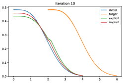
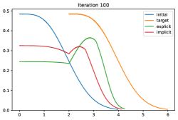
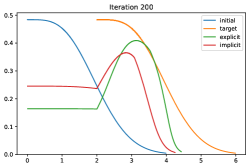
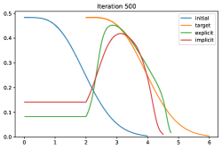
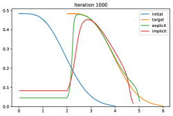
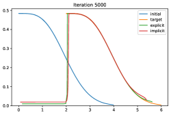
Figure 13: Comparison of implicit (red) and explicit (green) Euler schemes between $\mu_{0}\sim\mathcal{FN}(0,1)$ and $\nu\sim\mathcal{FN}(2,1)$ with $\tau=\tfrac{1}{100}$. For the corresponding quantile functions, see Figure 20.

Acknowledgments.

GS acknowledges funding by the German Research Foundation (DFG) within the project STE 571/16-1. JH acknowledges funding by the EPSRC programme grant The Mathematics of Deep Learning with reference EP/V026259/1.

Appendix A Additional Material

A.1 Supplement to Section 3

Remark A.1.

To be completely accurate, the set of quantile functions is the set of increasing and left-continuous functions (not equivalence classes) in $\mathcal{L}_{2}(0,1)$. However, each almost everywhere increasing function $f\in L_{2}(0,1)$ has a unique left-continuous representative: consider a function $\tilde{f}\in\mathcal{L}_{2}(0,1)$ in the equivalence class $f$, which is everywhere increasing. Then $\tilde{f}$ has at most countably many jump discontinuities $(s_{k})_{k\in\operatorname{\mathbb{N}}}$. Define $f_{0}\colon(0,1)\to\operatorname{\mathbb{R}}$ via $s\mapsto\lim_{t\uparrow s}\tilde{f}(t)$. Then $f_{0}$ differs from $\tilde{f}$ only at possibly $(s_{k})_{k\in\operatorname{\mathbb{N}}}$, and $f_{0}$ is increasing everywhere and left-continuous.

Indeed, $\operatorname{\mathcal{C}}(0,1)$ is closed, since for any sequence $(f_{n})_{n\in\operatorname{\mathbb{N}}}\subset\operatorname{\mathcal{C}}(0,1)$ converging to $f$ in $L_{2}(0,1)$ as $n\to\infty$, we have $f_{n}(s)\to f(s)$ along a subsequence for almost all $s\in(0,1)$. Since the pointwise limit of increasing functions is increasing, we see that $f\in\operatorname{\mathcal{C}}(0,1)$.

Proof of Proposition 3.4 Let $\lambda\in\operatorname{\mathbb{R}}$ and $F\colon L_{2}(0,1)\to\operatorname{\mathbb{R}}$ be $\lambda$-convex, that is,

$$F\left(tu+(1-t)v\right)\leq tF(u)+(1-t)F(v)-\frac{1}{2}\lambda t(1-t)\|u-v\|^{2}$$

for all $u,v\in\operatorname{dom}(F)\cap\operatorname{\mathcal{C}}(0,1)$ and all $t\in(0,1)$. Let $\gamma\colon[0,1]\to\operatorname{\mathcal{P}}_{2}(\operatorname{\mathbb{R}})$ be any geodesic with $\gamma_{0}=\mu$ and $\gamma_{1}=\nu$. Since $\mu\mapsto Q_{\mu}$ is an isometry by Theorem 3.2, the curve $t\mapsto Q_{\gamma_{t}}$ is a geodesic in $L_{2}(0,1)$. Since $L_{2}(0,1)$ is a linear space, the only geodesics are straight line segments, so we obtain

$$Q_{\gamma_{t}}=(1-t)Q_{\mu}+tQ_{\nu}.$$

Finally, we conclude

$$\operatorname{\mathcal{F}}(\gamma_{t}) =F(Q_{\gamma_{t}})=F\big{(}(1-t)Q_{\mu}+tQ_{\nu}\big{)}$$

$$\leq tF(Q_{\mu})+(1-t)F(Q_{\nu})-\frac{1}{2}\lambda t(1-t)\|Q_{\mu}-Q_{\nu}\|_{L_{2}(0,1)}^{2}$$

$$=t\operatorname{\mathcal{F}}(\mu)+(1-t)\operatorname{\mathcal{F}}(\nu)-\frac{1}{2}\lambda t(1-t)W_{2}^{2}(\mu,\nu).$$

The lower semicontinuity of $\mathcal{F}$ follows directly from the lower semicontinuity of $F$ using the isometric embedding, see Theorem 3.2. $\Box$

Theorem A.2 (Existence and regularity of strong solutions to (16) [9, Thm. 3.1, p. 54], [16]).

Let $H$ be a Hilbert space and $A\colon H\to 2^{H}$ be a maximal monotone operator. For all $g_{0}\in\operatorname{dom}(A)$, there exists a unique function $g\colon[0,\infty)\to H$ such that

1. $g(t)\in\operatorname{dom}(A)$ for all $t>0$,

2. $g$ is Lipschitz continuous on $[0,\infty)$, that is, $\frac{\mathop{}\!\mathrm{d}g}{\mathop{}\!\mathrm{d}t}\in L_{\infty}((0,\infty),H)$ (in the sense of distributions and in the strong sense a.e.) and

   $$\left\|\frac{\mathop{}\!\mathrm{d}g}{\mathop{}\!\mathrm{d}t}\right\|_{L_{\infty}((0,\infty),H)}\leq\|A^{\circ}g_{0}\|,$$

   where $A^{\circ}z\coloneqq\operatorname*{arg\,min}\{\|y\|:y\in Az\}$ denotes the minimal norm selection,

3. $\frac{\mathop{}\!\mathrm{d}g}{\mathop{}\!\mathrm{d}t}(t)\in-Ag(t)$ for almost all $t>0$,

4. $g(0)=g_{0}$.

Furthermore, $g$ satisfies the following properties:

1. $g$ admits a right derivative for all $t>0$ and $\frac{\mathop{}\!\mathrm{d}^{+}g}{\mathop{}\!\mathrm{d}t}(t)+A^{\circ}g(t)=0$ for all $t>0$,

2. $t\mapsto A^{\circ}g(t)$ is right-continuous and $t\mapsto\|A^{\circ}g(t)\|$ is decreasing.

3. $g$ is given by the exponential formula

   $$g(t)=\lim_{n\to\infty}\left(I+\frac{t}{n}A\right)^{-n}g_{0},$$ (74)

   uniformly in $t$ on compact intervals.

A.2 Supplement to Section 4

Proof of Proposition 4.2 The functional $F_{\nu}$ is convex, since for $u,v\in L_{2}(0,1)$ and $t\in(0,1)$ we have

$$F_{\nu}\big{(}tu+(1-t)v\big{)} =\int_{0}^{1}\bigg{(}(1-2s)\big{(}tu(s)+(1-t)v(s)-Q_{\nu}(s)\big{)}$$

$$+\int_{0}^{1}|tu(s)+(1-t)v(s)-Q_{\nu}(t)|\mathop{}\!\mathrm{d}{t}\bigg{)}\mathop{}\!\mathrm{d}{s}$$

$$\leq t\int_{0}^{1}\left((1-2s)\big{(}u(s)-Q_{\nu}(s)\big{)}+\int_{0}^{1}|u(s)-Q_{\nu}(t)|\mathop{}\!\mathrm{d}{t}\right)\mathop{}\!\mathrm{d}{s}$$

$$+(1-t)\int_{0}^{1}\left((1-2s)\big{(}v(s)-Q_{\nu}(s)\big{)}+\int_{0}^{1}|v(s)-Q_{\nu}(t)|\mathop{}\!\mathrm{d}{t}\right)\mathop{}\!\mathrm{d}{s}$$

$$=tF_{\nu}(u)+(1-t)F_{\nu}(v).$$

To show that $F_{\nu}$ is everywhere finite, notice that for all $u\in L_{2}(0,1)$,

$$|F_{\nu}(u)| \leq\int_{0}^{1}|1-2s||u(s)-Q_{\nu}(s)|+|u(s)|+\|Q_{\nu}\|_{L_{1}(0,1)}\mathop{}\!\mathrm{d}{s}$$

$$\leq 2(\|u\|_{L_{2}(0,1)}+\|Q_{\nu}\|_{L_{2}(0,1)})<\infty.$$

Lastly, we will show the continuity of $F_{\nu}$. Suppose that $(u_{n})_{n\in\operatorname{\mathbb{N}}}\subset L_{2}(0,1)$ converges to $u\in L_{2}(0,1)$. Then there exists a subsequence $(u_{n_{k}})_{k\in\operatorname{\mathbb{N}}}$ such that $u_{n_{k}}(s)\to u(s)$ for $k\to\infty$ for a.e. $s\in(0,1)$, and there exists a $m\in L_{1}(0,1)$ such that $|u_{n_{k}}(s)|\leq m(s)$ for a.e. $s\in(0,1)$.

Hence applying Lebesgue’s dominated convergence theorem twice yields

$$\lim_{k\to\infty}F_{\nu}(u_{n_{k}}) =\lim_{k\to\infty}\int_{0}^{1}\left((1-2s)\big{(}u_{n_{k}}(s)-Q_{\nu}(s)\big{)}+\int_{0}^{1}|u_{n_{k}}(s)-Q_{\nu}(t)|\mathop{}\!\mathrm{d}{t}\right)\mathop{}\!\mathrm{d}{s}$$

$$=F_{\nu}(u).$$

We can apply the dominated convergence theorem because in both cases the integrands are bounded above by an integrable function as follows: for almost all $s\in(0,1)$ we have by applying the triangle inequality many times that

$$\quad\left|(1-2s)\big{(}u_{n_{k}}(s)-Q_{\nu}(s)\big{)}+\int_{0}^{1}|u_{n_{k}}(s)-Q_{\nu}(t)|\mathop{}\!\mathrm{d}{t}\right|$$

$$\leq\underbrace{|1-2s|}_{\leq 1}|u_{n_{k}}(s)-Q_{\nu}(s)|+\int_{0}^{1}|u_{n_{k}}(s)-Q_{\nu}(t)|\mathop{}\!\mathrm{d}{t}$$

$$\leq|u_{n_{k}}(s)|+|Q_{\nu}(s)|+|u_{n_{k}}(s)|+\int_{0}^{1}|Q_{\nu}(t)|\mathop{}\!\mathrm{d}{t}$$

$$\leq 2m(s)+|Q_{\nu}(s)|+\|Q_{\nu}\|_{L_{1}(0,1)}.$$

This function is integrable because $m\in L_{1}(0,1)$ and $Q_{\nu}\in L_{2}(0,1)\subset L_{1}(0,1)$. Analogously, for any $s\in(0,1)$, the integrand $(0,1)\ni t\mapsto|u_{n_{k}}(s)-Q_{\nu}(t)|$ is bounded by the integrable function $t\mapsto|u_{n_{k}}(s)|+|Q_{\nu}(t)|$. $\Box$

A.3 Supplement to Section 6

Proof of Lemma 6.1 Let $s_{0}\in(0,1)$ be arbitrary and take a sequence $(s_{n})\subset(0,1)$ of values $s$ where (49) holds, and such that $s_{n}\uparrow s_{0}$. Then, it holds

$$h(s_{0})+\varepsilon s_{0}=\lim_{n\to\infty}h(s_{n})+\varepsilon s_{n}\geq\lim_{n\to\infty}u(s_{n})+\varepsilon R_{\nu}^{-}(u(s_{n}))=u(s_{0})+\varepsilon R_{\nu}^{-}(u(s_{0}))$$ (75)

by the left-continuity of $h$, $u$ and $R_{\nu}^{-}$, and since $u$ is increasing. Also, one has

$$h(s_{0})+\varepsilon s_{0}=\lim_{n\to\infty}h(s_{n})+\varepsilon s_{n}\leq\lim_{n\to\infty}u(s_{n})+\varepsilon R_{\nu}^{+}(u(s_{n}))\leq u(s_{0})+\varepsilon R_{\nu}^{+}(u(s_{0})),$$ (76)

since $R_{\nu}^{+}$ is upper semicontinuous. Since $s_{0}\in(0,1)$ was arbitrary, this shows the claim. $\Box$
Proof of Proposition 6.3 Let us write $R_{\mu}\coloneqq R_{\mu}^{+}$.
i) ’Only if’: Let $x,y\in R_{\mu}^{-1}((0,1))$ with $x>y$. W.l.o.g. suppose $R_{\mu}(x)>R_{\mu}(y)$ and let $\varepsilon>0$ such that $R_{\mu}(x)>R_{\mu}(y)+\varepsilon$. Then, it holds $Q_{\mu}(R_{\mu}(x))\leq x$ and $Q_{\mu}(R_{\mu}(y)+\varepsilon)>y$ by the Galois inequalities (12). Now, using that $Q_{\mu}\in D_{L,\text{low}}$, it follows that

$$L|R_{\mu}(x)-(R_{\mu}(y)+\varepsilon)| \leq|Q_{\mu}(R_{\mu}(x))-Q_{\mu}(R_{\mu}(y)+\varepsilon)|$$

$$=Q_{\mu}(R_{\mu}(x))-Q_{\mu}(R_{\mu}(y)+\varepsilon)$$

$$\leq x-y=|x-y|.$$

Letting $\varepsilon\downarrow 0$ shows

$$|R_{\mu}(x)-R_{\mu}(y)|\leq\frac{1}{L}|x-y|\quad\text{for all }x,y\in R_{\mu}^{-1}((0,1)).$$ (77)

Since $R_{\mu}\equiv 0$ on $R_{\mu}^{-1}((-\infty,0])$, $R_{\mu}\equiv 1$ on $R_{\mu}^{-1}([1,\infty))$, and since $R_{\mu}$ is continuous (on $\operatorname{\mathbb{R}}$) by Remark 3.1, $R_{\mu}$ is Lipschitz continuous on $\operatorname{\mathbb{R}}$ with constant $\leq L^{-1}$, which proves the ’only-if’ part.
’If’: Since $R_{\mu}$ is (Lipschitz) continuous, one has $R_{\mu}(Q_{\mu}(s))=s$ for all $s\in(0,1)$. It immediately follows

$$|Q_{\mu}(s_{1})-Q_{\mu}(s_{2})|\geq L|R_{\mu}(Q_{\mu}(s_{1}))-R_{\mu}(Q_{\mu}(s_{2}))|=L|s_{1}-s_{2}|$$ (78)

for all $s_{1},s_{2}\in(0,1)$, which concludes the proof of part i).
ii) ’Only if’: Since $Q_{\mu}$ is (Lipschitz) continuous, $R_{\mu}$ is strictly increasing on $R_{\mu}^{-1}((0,1))$ by Remark 3.1, and hence, $Q_{\mu}(R_{\mu}(x))=x$ for all $x\in R_{\mu}^{-1}((0,1))$. It immediately follows

$$|R_{\mu}(x)-R_{\mu}(y)|\geq\frac{1}{L}|Q_{\mu}(R_{\mu}(x))-Q_{\mu}(R_{\mu}(y))|=\frac{1}{L}|x-y|$$ (79)

for all $x,y\in R_{\mu}^{-1}((0,1))$. This inequality directly extends to all $x,y\in\overline{R_{\mu}^{-1}((0,1))}$, since $R_{\mu}$ is increasing.
’If’: Let $s_{1},s_{2}\in(0,1)$ with $s_{1}>s_{2}$. W.l.o.g. suppose $Q_{\mu}(s_{1})>Q_{\mu}(s_{2})$ and let $\varepsilon>0$ such that $Q_{\mu}(s_{1})-\varepsilon>Q_{\mu}(s_{2})$. Then, it holds $R_{\mu}(Q_{\mu}(s_{2}))\geq s_{2}$ and $R_{\mu}(Q_{\mu}(s_{1})-\varepsilon)<s_{1}$ by the Galois inequalities (12). Now, using the lower Lipschitz bound of $R_{\mu}$, it follows

$$\frac{1}{L}|(Q_{\mu}(s_{1})-\varepsilon)-Q_{\mu}(s_{2})| \leq|R_{\mu}(Q_{\mu}(s_{1})-\varepsilon)-R_{\mu}(Q_{\mu}(s_{2}))|$$

$$=R_{\mu}(Q_{\mu}(s_{1})-\varepsilon)-R_{\mu}(Q_{\mu}(s_{2}))$$

$$\leq s_{1}-s_{2}=|s_{1}-s_{2}|.$$

Letting $\varepsilon\downarrow 0$ shows $Q_{\mu}\in D_{L}$, which completes the proof of ii).
Finally, assume that $\mu$ is absolutely continuous. Then the bounds for its density follow by applying the fundamental theorem of calculus for absolutely continuous $R_{\mu}$, i.e., for all $x\geq y$,

$$|R_{\mu}(x)-R_{\mu}(y)|=R_{\mu}(x)-R_{\mu}(y)=\int_{y}^{x}f_{\mu}(\xi)\mathop{}\!\mathrm{d}\xi.\qquad\Box$$ (80)

A.4 Smoothness Properties: Different Approach

In the rest of this section, we highlight the statements from Section 6 from a different point of view. Instead of working with the exponential formula (17), we deal with the pointwise differential inclusion (40), allowing for a more direct approach.

The following theorem is analogous to Theorem 6.7. Let us remark that both theorems also hold true in a local sense, i.e., on subintervals $I\subseteq(0,1)$.

Theorem A.3.

Let $I\coloneqq(a,b)$ be such that $Q_{\mu_{0}}(I)\subset\operatorname{supp}\nu$. If $Q_{\mu_{0}}$ is locally upper Lipschitz on $I$ with constant $L_{\mu_{0}}\geq 0$, and if $R^{\pm}_{\nu}$ is locally lower Lipschitz on $\operatorname{conv}(Q_{\mu_{0}}(I)\cup Q_{\nu}(I))$ with constant $L_{\nu}^{-1}>0$, then $g(t)$ is locally upper Lipschitz on $I$ with

$${\rm Lip}(g(t))\leq L_{\mu_{0}}\,e^{-2tL_{\nu}^{-1}}+L_{\nu}\,(1-e^{-2tL_{\nu}^{-1}}).$$ (81)

Proof.

W.l.o.g. we consider $s_{1}<s_{2}$ in $I$ with $Q_{\mu_{0}}(s)<Q_{\nu}(s)$ for all $s_{1}\leq s\leq s_{2}$. Due to the local lower Lipschitz property of $R_{\nu}^{+}$, the derivatives of $g_{s_{1}}$ are bounded by

$$\dot{g}_{s_{1}}(t)=2s_{1}-2R_{\nu}^{+}(g_{s_{1}}(t))\geq 2L_{\nu}^{-1}(Q_{\nu}(s_{1})-g_{s_{1}}(t))$$

for almost every $t\geq 0$. Solving the differential equation with the lower bound and the initial value $Q_{\mu_{0}}(s_{1})$, we obtain

$$g_{s_{1}}(t)\geq Q_{\nu}(s_{1})+(Q_{\mu_{0}}(s_{1})-Q_{\nu}(s_{1}))\,e^{-2tL_{\nu}^{-1}}.$$ (82)

A similar procedure for $g_{s_{2}}$ yields

$$\dot{g}_{s_{2}}(t)=2s_{2}-2R^{+}_{\nu}(g_{s_{2}}(t))\leq 2s_{2}-2R^{+}_{\nu}(Q_{\mu_{0}}(s_{2})+2L_{\nu}^{-1}(Q_{\mu_{0}}(s_{2})-g_{s_{2}}(t))$$ (83)

and

$$g_{s_{2}}(t)\leq L_{\nu}(s_{2}-R^{+}_{\nu}(Q_{\mu_{0}}(s_{2})))+Q_{\mu_{0}}(s_{2})-L_{\nu}(s_{2}-R^{+}_{\nu}(Q_{\mu_{0}}(s_{2})))\,e^{-2tL_{\nu}^{-1}}.$$ (84)

Taking the difference and exploiting that

$$Q_{\mu_{0}}(s_{2})-Q_{\nu}(s_{1}) \leq L_{\nu}(R^{+}_{\nu}(Q_{\mu_{0}}(s_{2}))-R^{+}_{\nu}(Q_{\nu}(s_{1})))$$ (85)

$$\leq L_{\nu}(R^{+}_{\nu}(Q_{\mu_{0}}(s_{2}))-s_{1})$$ (86)

by the lower Lipschitz property of $R^{+}_{\nu}$, we obtain

$$\lvert g_{s_{2}}(t)-g_{s_{1}}(t)\rvert \leq(Q_{\mu_{0}}(s_{2})-Q_{\mu_{0}}(s_{1}))\,e^{-2tL_{\nu}^{-1}}$$ (87)

$$+(Q_{\mu_{0}}(s_{2})-Q_{\nu}(s_{1})+L_{\nu}s_{2}-L_{\nu}R^{+}_{\nu}(Q_{\mu_{0}}(s_{2}))\,(1-e^{-2tL_{\nu}^{-1}})$$ (88)

$$\leq(L_{\mu_{0}}\,e^{-2tL_{\nu}^{-1}}+L_{\nu}\,(1-e^{-2tL_{\nu}^{-1}}))\,(s_{2}-s_{1}).$$ (89)

∎

We can analogously argue for the lower Lipschitz property.

The following theorem is a counterpart to Theorem 6.11, but with a subtle difference in its nature: it states an invariance of the continuity in a single point $s\in(0,1)$, assuming in addition that $s$ is a continuity point of the target $Q_{\nu}$. On the other hand, Theorem 6.11 states an invariance of continuity on neighborhoods of $s$, without any further assumptions on the target.

Theorem A.4.

Let $s\in(0,1)$ be a continuity point of $Q_{\nu}$ and $Q_{\mu_{0}}$, then $g(t)$ is continuous at $s$ for all $t\geq 0$.

Proof.

Since $Q_{\nu}$ is continuous in $s$, for all $x<Q_{\nu}(s)$, there exists $\delta_{x}>0$ such that $\Phi_{\nu,s^{\prime}}(x)<\infty$ for all $s^{\prime}\in(s-\delta_{x},s+\delta_{x})$. The integrand of $\Phi_{\nu,s}$ is monotone in $s$ such that $\Phi_{\nu,s}(x)$ is continuous in $s$ due to Lebesgue’s dominated convergence theorem. To show that $g(t)$ is continuous in $s$, we use the $\epsilon$–$\delta$ criterion. First, we discuss the case $2t=\Phi_{\nu,s}(x)$ with $x<Q_{\nu}(s)$. For arbitrary $\epsilon>0$, we find $x_{1}\in(x-\epsilon,x)$ and $\delta_{1}>0$ such that $\Phi_{\nu,s^{\prime}}(x_{1})<2t$ for all $s^{\prime}\in(s-\delta_{1},s)$. Due to the monotonicity of $\Phi_{\nu,s}(x)$ in $s$, we have $\Phi_{\nu,s}^{-1}(2t)\in(x-\epsilon,x)$ for all $s^{\prime}\in(s-\delta_{1},s)$. Analogously, we find $x_{2}\in(x,x+\epsilon)$ and $\delta_{2}>0$ such that $\Phi_{\nu,s^{\prime}}(x_{2})$ is finite and $\Phi_{\nu,s^{\prime}}(x_{2})>2t$ for all $s^{\prime}\in(s,s+\delta_{2})$. Again due to the monotonicity, we have $\Phi_{\nu,s}^{-1}(2t)\in(x,x+\epsilon)$ for all $s^{\prime}\in(s,s+\delta_{2})$. Taking $\delta\coloneqq\min\{\delta_{1},\delta_{2}\}$, we finally have

$$[g(t)](s^{\prime})\in([g(t)](s)-\epsilon,[g(t)](s)+\epsilon)\quad\text{for all}\quad s^{\prime}\in(s-\delta,s+\delta).$$ (90)

Second, for the case $2t\geq\Phi_{\nu,s}(Q_{\nu}(s))$, we have to argue slightly differently. Here, we find $x_{1}\in(Q_{\nu}(s)-\epsilon,Q_{\nu}(s))$ and $\delta_{1}>0$ such that $\Phi_{\nu,s^{\prime}}(x_{1})<2t$ and thus $\Phi_{\nu,s^{\prime}}^{-1}(2t)>Q_{\nu}(s)-\epsilon$ for all $s^{\prime}\in(s-\delta_{1},s+\delta_{1})$. Due to the continuity of the target $Q_{\nu}$ in $s$, we find $\delta_{2}>0$ such that $Q_{\nu}(s^{\prime})<Q_{\nu}(s)+\epsilon)$ for all $s^{\prime}\in(s-\delta_{2},s+\delta_{2})$. Taking $\delta\coloneqq\min\{\delta_{1},\delta_{2}\}$, we again have

$$[g(t)](s^{\prime})\in([g(t)](s)-\epsilon,[g(t)](s)+\epsilon)\quad\text{for all}\quad s^{\prime}\in(s-\delta,s+\delta).$$ (91)

∎

A.5 Quantile functions plots for the experiments

In this supplementary section we plot the quantile functions belonging to the densities in figures 4 and 8 – 13 from the main text.

Here, one can nicely verify the results from the previous subsection, in particular, that a pointwise view on the Cauchy problem on quantile functions is insightful.

In the fully discrete case, see Figure 14, we have $Q_{\mu_{0}}\not\in D_{c}$, and so we can not apply Theorem 6.11 i). In fact, $Q_{\gamma_{t}}\not\in D_{c}$ for all $t\geq 0$.

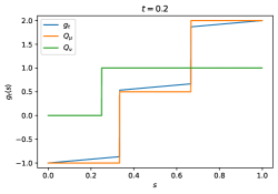
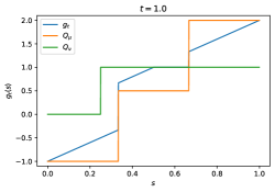
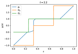
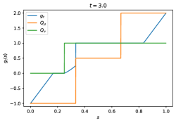
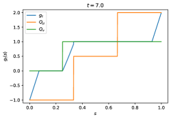
Figure 14: The quantile functions of the Wasserstein gradient flow between the point measures in Example 5.4. For the corresponding densities, see Figure 4.

Concerning the examples with absolutely continuous target, plotted in figures 15 – 20, we observe that the quantile functions differ mostly at the boundary, that is, for values of $s$ close to zero or close to one. Furthermore, we observe that Proposition 6.4 holds true, i.e., the range of the quantile functions $Q_{\gamma_{t}}$ does not leave the range of $Q_{\mu_{0}}$ and $Q_{\nu}$, and we can verify the monotonicity of the ranges of $Q_{\gamma_{t}}$ predicted by Theorem 6.11 ii). We also see that Theorem 6.11 holds true: the quantile functions stay continuous because $g_{0}=Q_{\mu_{0}}$ is continuous. Lastly, we have ${\rm Lip}(Q_{\mu_{0}})=\infty$ in all these examples, so Theorem 6.7 does not apply. Indeed, $Q_{\gamma_{t}}\not\in D_{L}^{+}$ for all $L>0$.

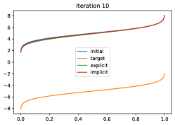
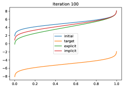
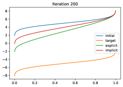
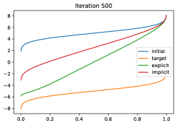
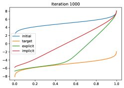
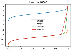
Figure 15: Comparison of the quantile functions belonging to the implicit (red) and explicit (green) Euler schemes between two Gaussians $\mu_{0}\sim\operatorname{\mathcal{N}}(5,1)$ and $\nu\sim\operatorname{\mathcal{N}}(-5,1)$ with $\tau=\tfrac{1}{100}$. For the corresponding densities, see Figure 8.

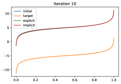
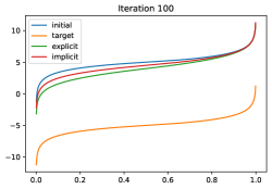
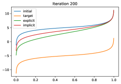
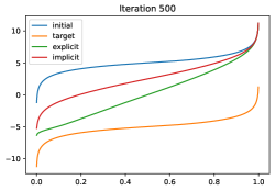
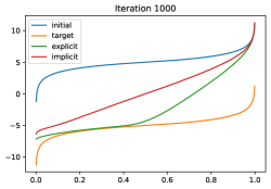
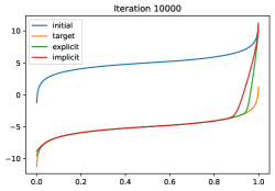
Figure 16: Comparison of the quantile functions belonging to the implicit (red) and explicit (green) Euler schemes between two Laplacians $\mu_{0}\sim\mathcal{L}(5,1)$ and $\nu\sim\mathcal{L}(-5,1)$ with $\tau=\tfrac{1}{100}$. For the corresponding densities, see Figure 9.

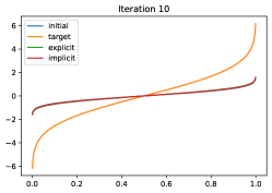
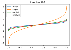
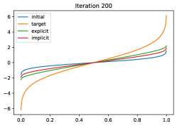
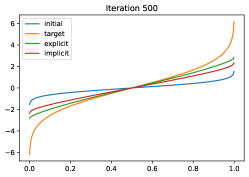
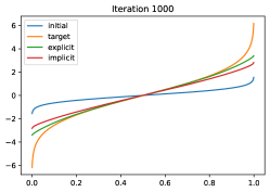
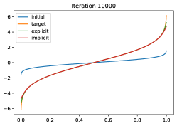
Figure 17: Comparison of the quantile functions belonging to the implicit (red) and explicit (green) Euler schemes between two Gaussians $\mu_{0}\sim\operatorname{\mathcal{N}}(0,\sqrt{2})$ and $\nu\sim\operatorname{\mathcal{N}}(0,\tfrac{1}{\sqrt{2}})$ with $\tau=\tfrac{1}{100}$. For the corresponding densities, see Figure 10.

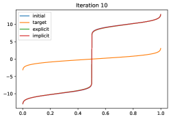
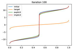
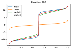
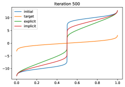
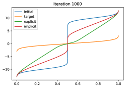
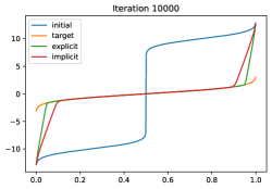
Figure 18: Comparison of of the quantile functions belonging to the implicit (red) and explicit (green) Euler schemes between $\mu_{0}\sim\frac{1}{2}\operatorname{\mathcal{N}}(-10,1)+\frac{1}{2}\operatorname{\mathcal{N}}(10,1)$ and $\nu\sim\operatorname{\mathcal{N}}(0,1)$ with $\tau=\tfrac{1}{100}$. For the corresponding densities, see Figure 11.

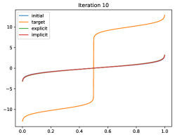
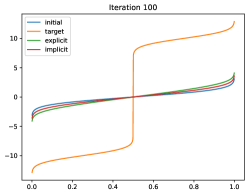
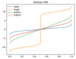
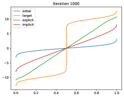
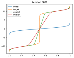
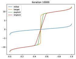
Figure 19: Comparison of implicit (red) and explicit (green) Euler schemes between $\mu_{0}\sim\operatorname{\mathcal{N}}(0,1)$ and $\nu\sim\frac{1}{2}\operatorname{\mathcal{N}}(-10,1)+\frac{1}{2}\operatorname{\mathcal{N}}(10,1)$ with $\tau=\tfrac{1}{100}$. For the corresponding densities, see Figure 12.

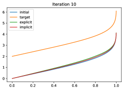
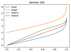
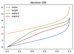
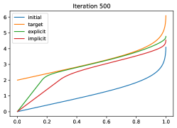
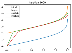
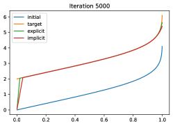
Figure 20: Comparison of the quantile functions belonging to the implicit (red) and explicit (green) Euler schemes between $\mu_{0}\sim\mathcal{FN}(0,1)$ and $\nu\sim\mathcal{FN}(2,1)$ with $\tau=\tfrac{1}{100}$. For the corresponding densities, see Figure 13.

A.6 Implicit Euler Scheme for the Flow Towards $\delta_{0}$ Starting in a Uniform or Gaussian Measure

Let $\nu=\delta_{0}$. Then the multi-valued operator $I+2\tau[R_{\nu}^{-},R_{\nu}^{+}]$ appearing on the left hand side of (72) is given by

$$\operatorname{\mathbb{R}}\ni x\mapsto x+2\tau[R_{\nu}^{-}(x),R_{\nu}^{+}(x)]=\begin{cases}x,&\text{if }x<0,\\ [0,2\tau],&\text{if }x=0,\\ x+2\tau,&\text{if }x>0,\end{cases}$$

and its inverse is given by $S_{\tau}(\cdot-\tau)$, where

$$S_{\tau}\colon\operatorname{\mathbb{R}}\to\operatorname{\mathbb{R}},\qquad x\mapsto\begin{cases}x+\tau,&\text{if }x<-\tau,\\ 0,&\text{if }-\tau\leq x\leq\tau,\\ x-\tau,&\text{if }x>\tau,\end{cases}$$

is the soft-shrinkage operator with threshold $\tau>0$.

Thus the implicit Euler scheme on quantile functions is given by the simple update

$$g_{n+1}(s)=S_{\tau}(g_{n}(s)+2\tau s-\tau).$$

For a uniform initial distribution and for a Gaussian initial distribution, these iterates are displayed in Figure 21.

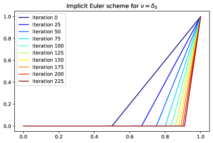
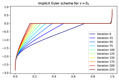
Figure 21: Iterates (quantile functions) of the implicit Euler scheme (16) with $\nu=\delta_{0}$ and $\tau=\tfrac{1}{100}$ starting in $\mu_{0}\sim\mathcal{U}[0,1]$ (left) and $\mu_{0}\sim\operatorname{\mathcal{N}}(-1,0.5)$ (right).

References

- [1] L. Ambrosio, N. Gigli, and G. Savare. Gradient Flows. Lectures in Mathematics ETH Zürich. Birkhäuser, Basel, 2nd edition, 2008.
- [2] M. Arbel, A. Korba, A. Salim, and A. Gretton. Maximum mean discrepancy gradient flow. In Advances in Neural Information Processing Systems, volume 32, 2019.
- [3] H. Bauschke and P. Combettes. Convex Analysis and Monotone Operator Theory in Hilbert Spaces. CMS Books in Mathematics. Springer New York, 2011.
- [4] J. Benedetto and W. Czaja. Integration and Modern Analysis. Birkhäuser, Boston, 2009.
- [5] A. Berdellima and G. Steidl. Quasi-alpha firmly nonexpansive mappings in Wasserstein spaces. Fixed Point Theory, arXiv:2203.04851, 2024.
- [6] G. A. Bonaschi. Gradient flows driven by a non-smooth repulsive interaction potential. Master’s thesis, University of Pavia, 2013.
- [7] G. A. Bonaschi, J. A. Carrillo, M. Di Francesco, and M. A. Peletier. Equivalence of gradient flows and entropy solutions for singular nonlocal interaction equations in 1d. ESAIM: Control, Optimisation and Calculus of Variations, 21(2):414–441, 2015.
- [8] S. Boufadène and F.-X. Vialard. On the global convergence of Wasserstein gradient flow of the Coulomb discrepancy. arXiv preprint arXiv:2312.00800, 2023.
- [9] H. Brezis. Operateurs Maximaux Monotones. North-Holland Mathematics Studies, 1973.
- [10] M. Burger and M. Di Francesco. Large time behavior of nonlocal aggregation models with nonlinear diffusion. Networks and Heterogeneous Media, 3(4):749–785, 2008.
- [11] J. A. Carrillo, Y.-P. Choi, and M. Hauray. The derivation of swarming models: Mean-field limit and Wasserstein distances. In A. Muntean and F. Toschi, editors, Collective Dynamics from Bacteria to Crowds: An Excursion Through Modeling, Analysis and Simulation, pages 1–46. Springer Vienna, Vienna, 2014.
- [12] J. A. Carrillo, M. Di Francesco, A. Esposito, S. Fagioli, and M. Schmidtchen. Measure solutions to a system of continuity equations driven by Newtonian nonlocal interactions. Discrete and Continuous Dynamical Systems, 40(2):1191–1231, 2020.
- [13] J. A. Carrillo, D. Slepčev, and L. Wu. Nonlocal-interaction equations on uniformly prox-regular sets. Discrete and Continuous Dynamical Systems, 36(3):1209–1247, 2016.
- [14] D. Chafaï, R. Matzke, E. Saff, M. Vu, and R. Womersley. Riesz energy with a radial external field: When is the equilibrium support a sphere? arXiv preprint arXiv:2405.00120, 2024.
- [15] Y. Chen, D. Z. Huang, J. Huang, S. Reich, and A. M. Stuart. Sampling via gradient flows in the space of probability measures. arXiv preprint arXiv:2310.03597, 2023.
- [16] M. G. Crandall and T. M. Liggett. Generation of semi-groups of nonlinear transformations on general banach spaces. American Journal of Mathematics, 93(2):265–298, 1971.
- [17] H. Daneshmand and F. Bach. Polynomial-time sparse measure recovery: From mean field theory to algorithm design. arXiv preprint arXiv:2204.07879, 2022.
- [18] H. Daneshmand, J. D. Lee, and C. Jin. Efficient displacement convex optimization with particle gradient descent. In International Conference on Machine Learning, pages 6836–6854. PMLR, 2023.
- [19] M. Di Francesco. Scalar conservation laws seen as gradient flows: known results and new perspectives. ESAIM: Proceedings and Surveys, 54:18–44, 2016.
- [20] M. Di Francesco, S. Fagioli, and E. Radici. Measure solutions, smoothing effect, and deterministic particle approximation for a conservation law with nonlocal flux. arXiv preprint arXiv:2406.03837, 2024.
- [21] K. Fellner and G. Raoul. Stability of stationary states of non-local equations with singular interaction potentials. Mathematical and Computer Modelling, 53(7):1436–1450, 2011.
- [22] M. Fornasier, J. Haskovec, and G. Steidl. Consistency of variational continuous-domain quantization via kinetic theory. Applicable Analysis, 92(6):1283–1298, 2013.
- [23] P. Hagemann, J. Hertrich, F. Altekrüger, R. Beinert, J. Chemseddine, and G. Steidl. Posterior sampling based on gradient flows of the MMD with negative distance kernel. In International Conference on Learning Representations, 2024.
- [24] J. Hertrich, R. Beinert, M. Gräf, and G. Steidl. Wasserstein gradient flows of the discrepancy with distance kernel on the line. In International Conference on Scale Space and Variational Methods in Computer Vision, pages 431–443. Springer, 2023.
- [25] J. Hertrich, M. Gräf, R. Beinert, and G. Steidl. Wasserstein steepest descent flows of discrepancies with Riesz kernels. Journal of Mathematical Analysis and Applications, 531(1):127829, 2024.
- [26] J. Hertrich, C. Wald, F. Altekrüger, and P. Hagemann. Generative sliced MMD flows with Riesz kernels. In International Conference on Learning Representations, 2024.
- [27] Y. Huang, E. Mainini, J. L. Vázquez, and B. Volzone. Nonlinear aggregation-diffusion equations with Riesz potentials. Journal of Functional Analysis, 287(2):110465, 2024.
- [28] R. Jordan, D. Kinderlehrer, and F. Otto. The variational formulation of the Fokker–Planck equation. SIAM Journal on Mathematical Analysis, 29(1):1–17, 1998.
- [29] R. Laumont, V. Bortoli, A. Almansa, J. Delon, A. Durmus, and M. Pereyra. Bayesian imaging using plug & play priors: when Langevin meets Tweedie. SIAM Journal on Imaging Sciences, 15(2):701–737, 2022.
- [30] H. Li and G. Toscani. Long-time asymptotics of kinetic models of granular flows. Archive for Rational Mechanics and Analysis, 172:407–428, 2004.
- [31] F. Maggi. Optimal Mass Transport on Euclidean Spaces. Cambridge Studies in Advanced Mathematics. Cambridge University Press, 2023.
- [32] E. Naldi and G. Savaré. Weak topology and Opial property in Wasserstein spaces with applications to gradient flows and proximal point algorithms of geodesically convex functionals. Rendiconti Lincei Matematica e Applicazioni, 32(4):725–750, 2022.
- [33] P. I. Natanson. Theory of Functions of a Real Variable. Ungar, New York, 1955.
- [34] J. Peypouquet and S. Sorin. Evolution equations for maximal monotone operators: Asymptotic analysis in continuous and discrete time. Journal of Convex Analysis, 17(3&4):1113–1163, 2010.
- [35] R. T. Rockafellar. Integrals which are convex functionals. II. Pacific Journal of Mathematics, 39(2):439–469, 1971.
- [36] R. T. Rockafellar and J. O. Royset. Random variables, monotone relations, and convex analysis. Mathematical Programming, 148:297–331, 2014.
- [37] O. Scherzer, M. Grasmair, H. Grossauer, M. Haltmeier, and F. Lenzen. Variational Methods in Imaging, volume 167. Springer, 2009.
- [38] D. Sejdinovic, B. Sriperumbudur, A. Gretton, and K. Fukumizu. Equivalence of distance-based and RKHS-based statistics in hypothesis testing. The Annals of Statistics, 41(5):2263 – 2291, 2013.
- [39] G. Székely. E-statistics: The energy of statistical samples. Techical Report, Bowling Green University, 2002.
- [40] G. J. Székely and M. L. Rizzo. Energy statistics: A class of statistics based on distances. Journal of Statistical Planning and Inference, 143(8):1249–1272, 2013.
- [41] C. Villani. Topics in Optimal Transportation. Number 58 in Graduate Studies in Mathematics. American Mathematical Society, Providence, 2003.
- [42] C. Villani. Optimal Transport. Springer, Berlin, 2009.