-Exponential Family For Policy Optimization
Abstract
Policy optimization methods benefit from a simple and tractable policy functional, usually the Gaussian for continuous action spaces. In this paper, we consider a broader policy family that remains tractable: the -exponential family. This family of policies is flexible, allowing the specification of both heavy-tailed policies () and light-tailed policies (). This paper examines the interplay between -exponential policies for several actor-critic algorithms conducted on both online and offline problems. We find that heavy-tailed policies are more effective in general and can consistently improve on Gaussian. In particular, we find the Student’s t-distribution to be more stable than the Gaussian across settings and that a heavy-tailed -Gaussian for Tsallis Advantage Weighted Actor-Critic consistently performs well in offline benchmark problems. Our code is available at https://github.com/lingweizhu/qexp.
1 Introduction
†† These authors contributed equally to this work.Policy optimization methods optimize the parameters of a stochastic policy towards maximizing some performance measure (Sutton et al., 1999). These methods benefit from a simple and tractable policy functional. For discrete action spaces, the Boltzmann-Gibbs (BG) policy is often preferred (Mei et al., 2020; Cen et al., 2022); while the Gaussian policy is standard for the continuous case. Gaussian can be recovered from the continuous BG provided that action value function is parametrized as a negative quadratic function. For continuous action spaces, evaluating BG is generally intractable due to the normalizing log-partition function. Gaussian policy is often used as a tractable approximation: being a member of the location-scale family, it is simple to implement, and can be easily generalized to multi-dimensional case. While there are other candidates such as the Beta policy (Chou et al., 2017), Gaussian remains the most common choice for both online and offline policy optimization methods (Haarnoja et al., 2018; Neumann et al., 2023; Xiao et al., 2023).
In this paper, we consider a broader policy family that remains tractable called the -exponential family. The motivation lies in (1) the need for strong exploration capability and error tolerance that match the original BG (Ahmed et al., 2019; Vieillard et al., 2020). (2) consistency between theory and practice: some algorithms are derived based on non-exp policies that may have more sparse or heavier tails, and using Gaussian incurs a mismatch (Lee et al., 2020; Zhu et al., 2024).
-exponential family was proposed to study non-extensive system behaviors in the statistical physics (Naudts, 2010; Matsuzoe and Ohara, 2011), and has recently been exploited in the attention-based methods (Peters et al., 2019; Martins et al., 2022). By setting , it recovers the standard exponential family. With , we can obtain policies with heavier tails than the Gaussian, such as the Student’s t-distribution. Heavy-tailed distributions could be more preferable as they are more robust (Lange et al., 1989), can facilitate exploration and help escape local optima (Kobayashi, 2019). When , light-tailed (sparse) policies such as the -Gaussian distribution can be recovered. Sparse -Gaussian has finite support and can serve as a continuous generalization of the discrete sparsemax. As a result, -Gaussian may help alleviate the bias and safety concerns incurred by infinite support Gaussian policies (Chou et al., 2017; Xu et al., 2023; Li et al., 2023).
In short, the contributions of this paper are: (1) we introduce the general -exponential family policies as potential substitutes for the Gaussian. We motivate the -exp family by the Tsallis regularization; (2) comprehensive experiments on both online and offline problems show that the -exp family policies can improve on Gaussian by a large margin. In particular, the Student’s t policy is more stable performing across settings thanks to its learnable degree of freedom parameter; (3) our empirical results align with the assumption that algorithms may prefer specific policies depending on the actor loss objective. For instance, by replacing Gaussian with heavy-tailed -Gaussian, Tsallis advantage weighted actor-critic (Zhu et al., 2024) consistently performs favorably in offline benchmark problems.
| Reference | Definition of | Continuous? | Literature |
| Lee et al. (2018); Chow et al. (2018) | ✗ | RL | |
| Lee et al. (2020); Zhu et al. (2024) | ✗ | RL | |
| Zhu et al. (2023) | ✗ | RL | |
| Li et al. (2023) | ✓ | RL | |
| Naudts (2010) | , General -exp family | ✓ | Physics |
| Martins et al. (2022) | , Light-tailed -exp family | ✓ | ML |
| This paper | , General -exp family | ✓ | RL |
Remark.
There are two possible definitions of the -exp function in existing works, see Table 1. The definition is used more frequently in the physics and machine learning (ML) literature, and has been used by some authors in the RL context. Lee et al. (2018); Chow et al. (2018) considered discrete policy , see Section 3 for notations. It corresponds to in (Lee et al., 2020; Zhu et al., 2024). Li et al. (2023) considered -Gaussian but with a specific . This paper follows the convention, and is the first to consider general, continuous -exp family policies including both the light-tailed and heavy-tailed distributions.
2 Background
We focus on discounted Markov Decision Processes (MDPs) expressed by the tuple , where and denote state space and finite action space, respectively. Let denote the set of probability distributions over . denotes the transition probability function, and defines the reward associated with that transition. is the discount factor. A policy is a mapping from the state space to distributions over actions. To assess the quality of a policy, we define the expected return as , where is the unnormalized state visitation frequency. The goal is to learn a policy that maximizes . We also define the action value and state value as , .
For notational convenience, we define the inner product for any two functions over actions as . We write to express the dependency of the function on state . Often , whenever its component is of concern, we denote it by .
In practice, the policy is often parametrized by a vector of parameters . The policy then can be optimized by adjusting its parameters towards high reward region utilizing its gradient information. The Policy Gradient Theorem (Sutton et al., 1999) featured by many state-of-the-art policy gradient methods states that the gradient can be computed by:
In practice, the expectation is approximated by sampling. When the state space is large, the action value function is also parametrized, leading to the Actor-Critic methods (Degris et al., 2012).
In contrast to the popular policy gradient algorithms, how specific policy functionals affect the performance remains a less studied topic. Researchers usually use the Gaussian policy which gives the gradients and . On one hand, as a member of the location-scale family, Gaussian policy is simple to implement. On the other hand, when becomes small, Gaussian can be unstable due to overly large gradients and can prematurely concentrate on a suboptimal action. As a result, it is susceptible to noise/outliers and does not encourage sufficient exploration due to its thin tails. In this paper, we investigate location-scale alternatives within the generalized -exponential family.
3 Exponential and -Exponential Families
We first review commonly used exponential family policies. By deforming the exponential function, we arrive at the more general -exponential family that includes both heavy-tailed and light-tailed (sparse) policies. In Table 2 we summarize all policies presented in the paper.
| Family | Policy | Notation | Parameters | Statistics | Normalization |
| Boltzmann-Gibbs | - | ||||
| Gaussian | |||||
| Beta | |||||
| - | Sparsemax | - | |||
| Student’s t | |||||
| -Gaussian | |||||
| -Gaussian |
3.1 The Exponential Family, Boltzmann-Gibbs and Gaussian Policies
Consider a class of policies given by the exponential family:
| (1) |
Here, is a vector of statistics and is a vector of parameters, is the normalizing constant ensuring the policy is a valid distribution.
It is clear that by assuming with denoting the temperature parameter, we recover the Boltzmann-Gibbs (BG) policy , where is the log-partition function. In the discrete case, it is also called the softmax transformation (Cover and Thomas, 2006). BG policy has been studied extensively in RL for encouraging exploration, facilitating the exploration-exploitation trade-off, and smoothing optimization landscape, to name a few applications (Haarnoja et al., 2018; Ahmed et al., 2019; Mei et al., 2020; Cen et al., 2022). It is worth noting that BG can be multi-modal depending on . In continuous action spaces, evaluating the log-partition function is in general intractable, though there are some recent research attempts on sidestepping its direct evaluation (Garg et al., 2023).
Gaussian policy is frequently used for continuous action spaces. To see it is a member of the exponential family, let for ; , and . This amounts to setting in BG (Gu et al., 2016). We write a Gaussian policy as . Typically, is parametrized by a neural network such that actions are sampled from .
Another interesting member is the Beta distribution (Chou et al., 2017): , where is the gamma function. It can be retrieved from Eq. (1) by letting , . Since Beta distribution’s support is bounded between , Chou et al. (2017) argued that it may alleviate the bias brought by truncating Gaussian densities outside the action space bounds. Beta policy is the only non-location-scale family distribution in this paper. As will be shown in the experiments, Beta policy does not perform favorably against Gaussian in general.
3.2 The -Exponential Family, Heavy-tailed and Light-tailed Policies
Generalizing the exponential family using deformed exponential functions has been extensively discussed in statistical physics (Naudts, 2002; Tsallis, 2009; Naudts, 2010; Amari and Ohara, 2011). In the machine learning literature, the -exponential generalization has attracted some attention since it allows for tuning the tail behavior by (Sears, 2008; Ding and Vishwanathan, 2010; Amid et al., 2019). The -exponential and its unique inverse function -logarithm are defined by:
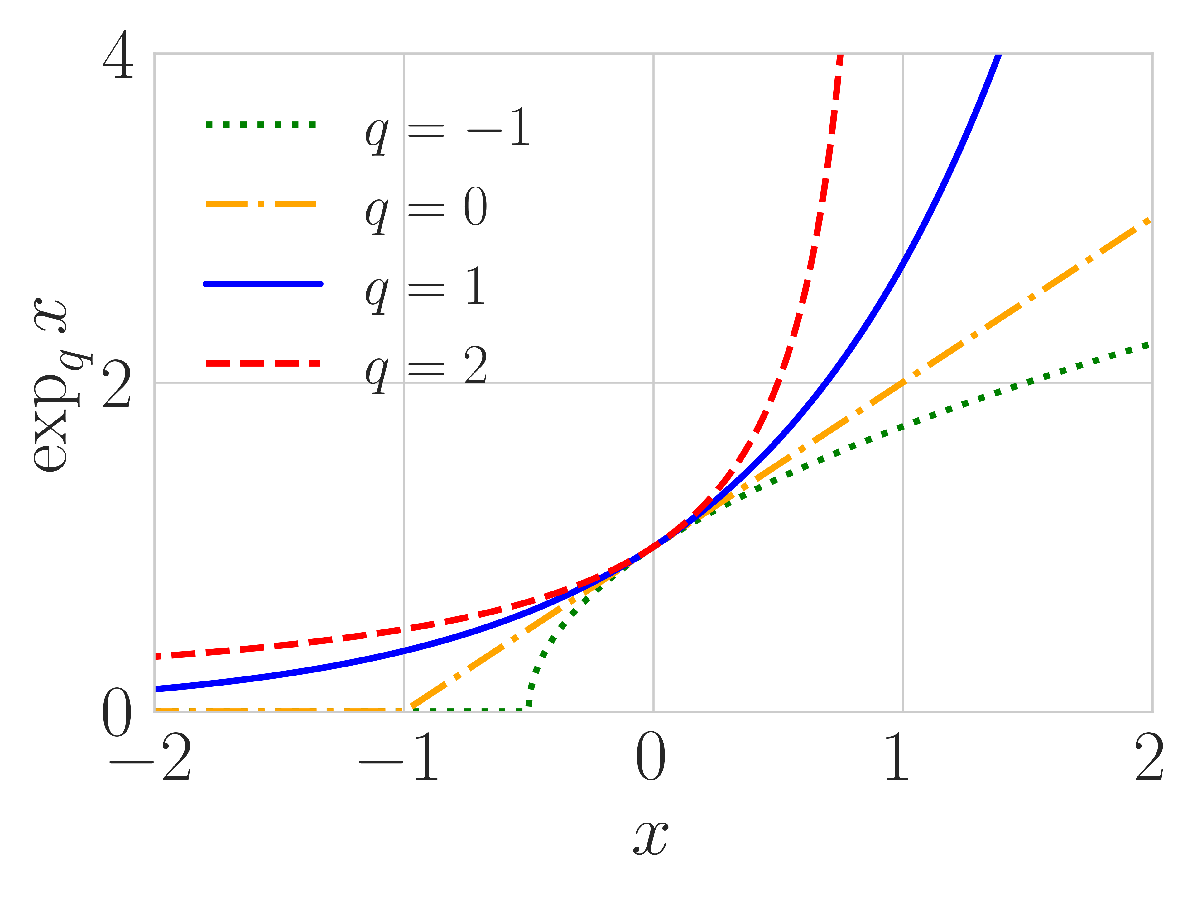
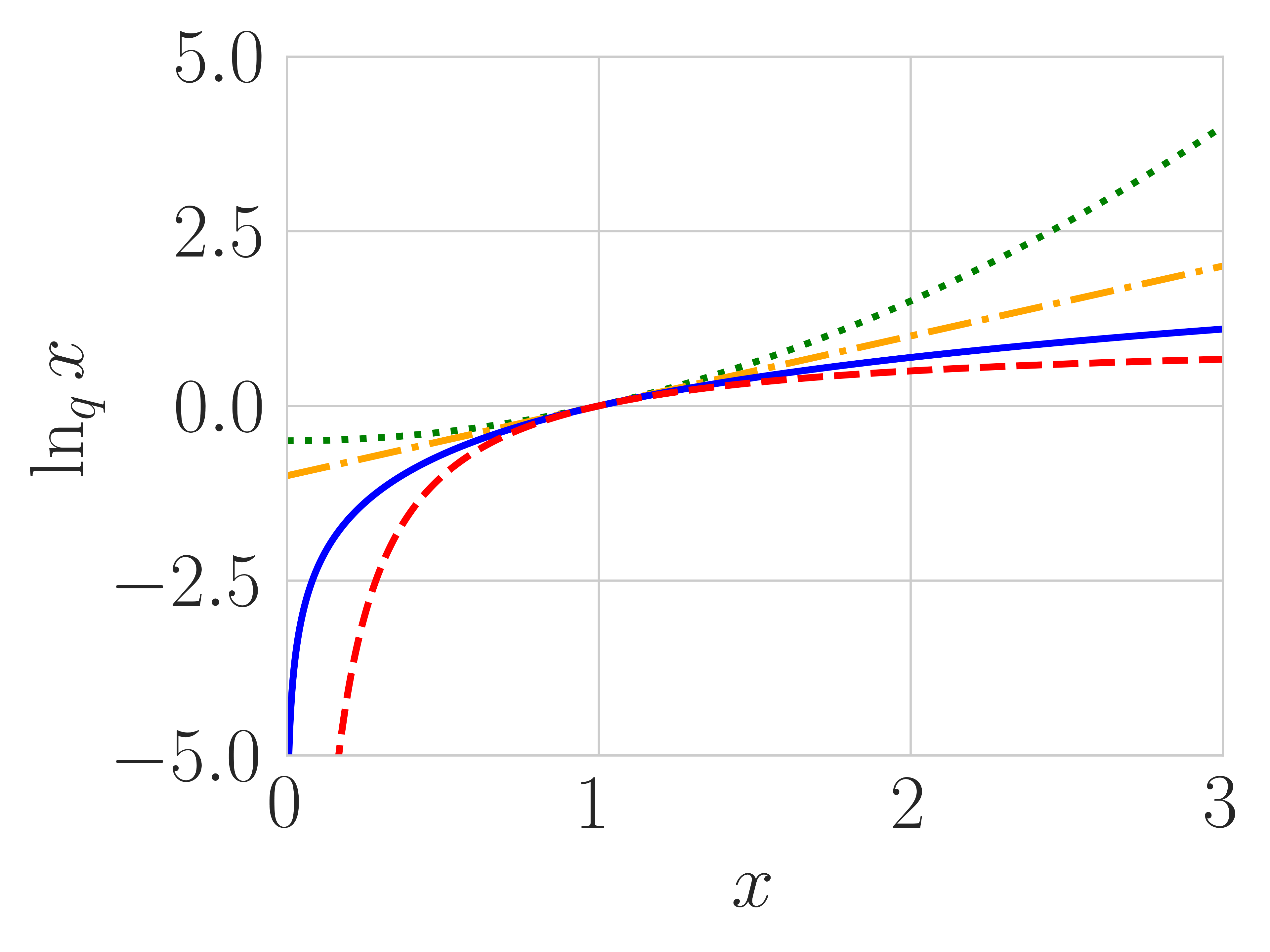
| (2) |
where . -exp/log generalize exp/log since and . Similar to exp, -exp is an increasing and convex function for , satisfying . However, an important difference of -exp is that unless . We visualize -exp/log in Figure 1.
We now define the -exponential family policy as:
| (3) |
Where have similar meanings to Eq.(1). Note that unless , see Eq.(5). The -exponential family includes the following well-known distributions.
3.2.1 Light-tailed Policy ()
One prominent example of this class is the discrete sparsemax policy (Martins and Astudillo, 2016), recovered when and : . assigns probabilities only to a subset of actions by adaptively calculating the threshold: , where is the set of highest-valued actions satisfying , with denoting the action with th largest value. Sparsemax policies have been generalized to the domain of (Lee et al., 2020; Zhu et al., 2023), though there is no analytic when and hence approximation is required.
For a continuous policy, Li et al. (2023) considered the following specific instance of -Gaussian (we define it more formally in Eq. (6)): , where we used to denote -Gaussian; the normalization in this case is . We can see that it is indeed a -exp policy with and . More generally, we can assume with . Then .
3.2.2 Heavy-tailed Policy ()
It is well-known that animals searching for feed exhibit heavy-tailed behaviors called the Lévy flight (Bartumeus et al., 2005). Heavy-tailed distributions like the Student’s-t are popular for robust modelling (Lange et al., 1989):
| (4) |
where is the degree of freedom. As , Student’s t distribution approaches Gaussian. Numerically, Student’s t with is considered to match Gaussian. Therefore, can be an important learnable parameter in addition to its location and scale . It allows the policy to adaptively balance the exploration-exploitation trade-off by interpolating the Gaussian and heavy-tailed policies. Now let , i.e. and define
| (5) | ||||
which we see it is indeed a -exp policy. In this case we see that . Student’s t policy has been used in (Kobayashi, 2019) to encourage exploration and escaping local optima. Another related case is the Cauchy’s distribution recovered when (or from Student’s t). Cauchy’s distribution can be used as the starting point for learning Student’s t, see Appendix B.2 for details. Note that Cauchy’s distribution does not have valid mean, variance or any higher moments.
3.2.3 -Gaussian
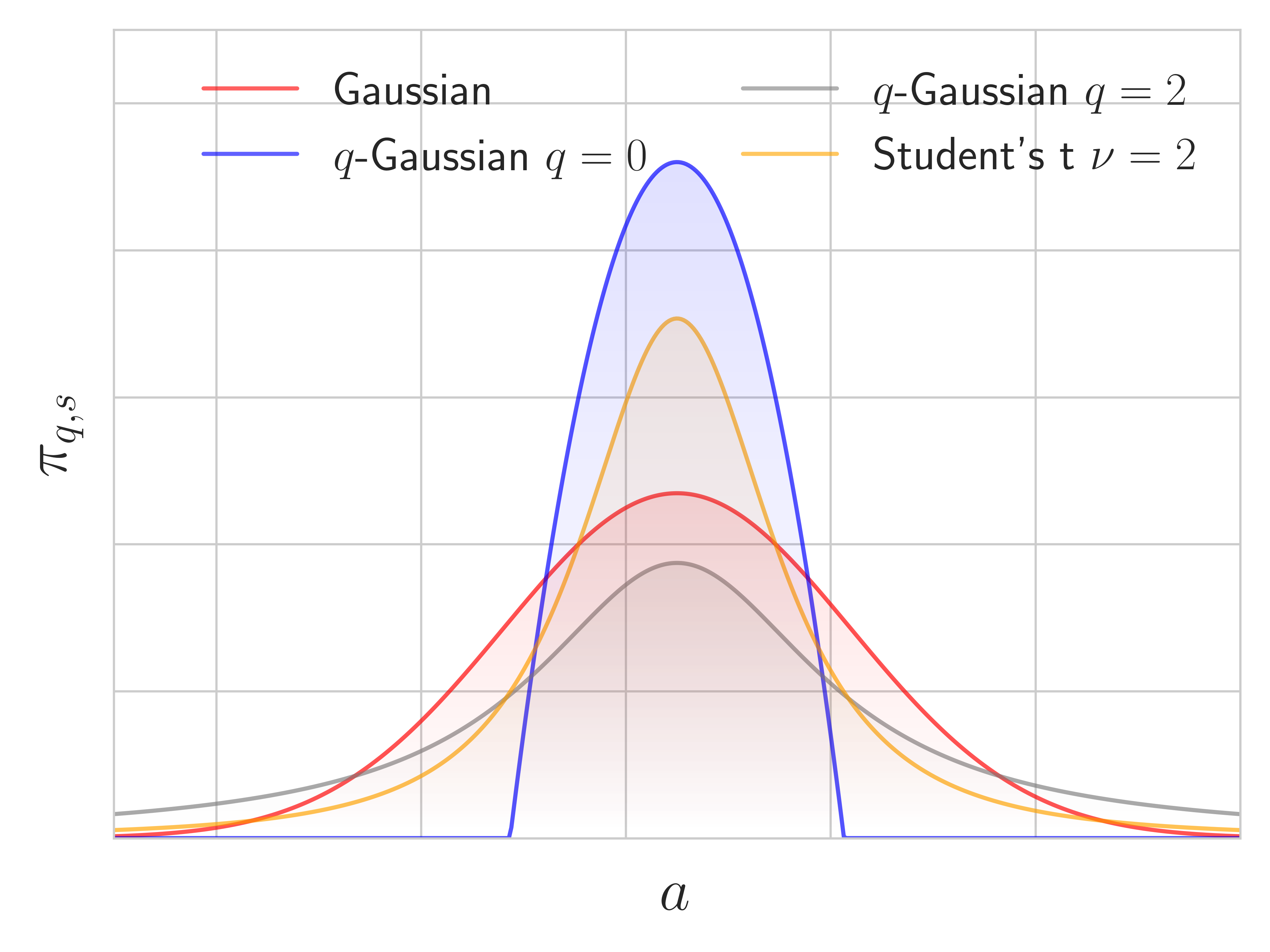
As the counterpart of Gaussian in the -exp family, -Gaussian unifies both light-tailed and heavy-tailed policies by varying (Matsuzoe and Ohara, 2011):
| (6) | ||||
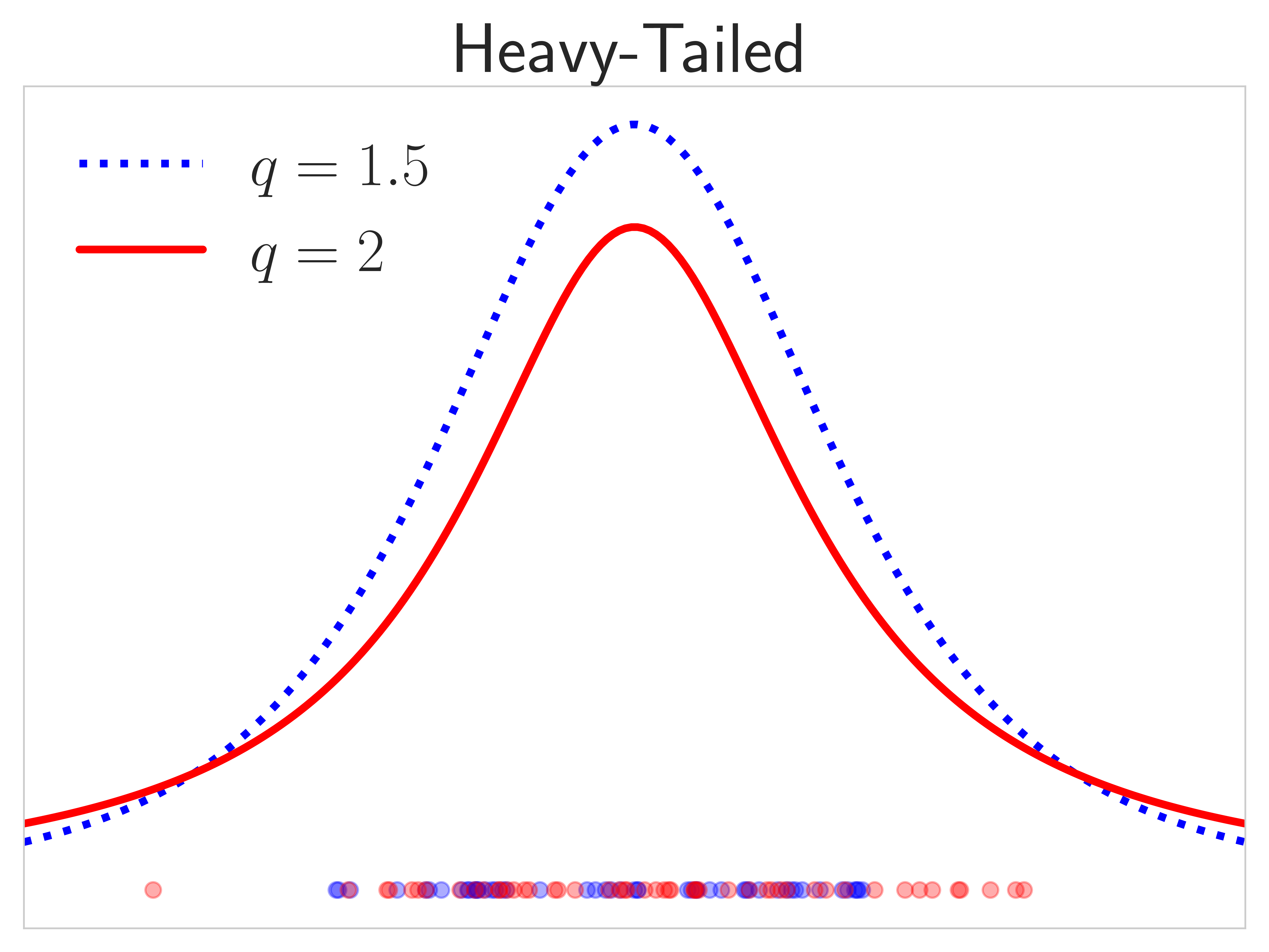
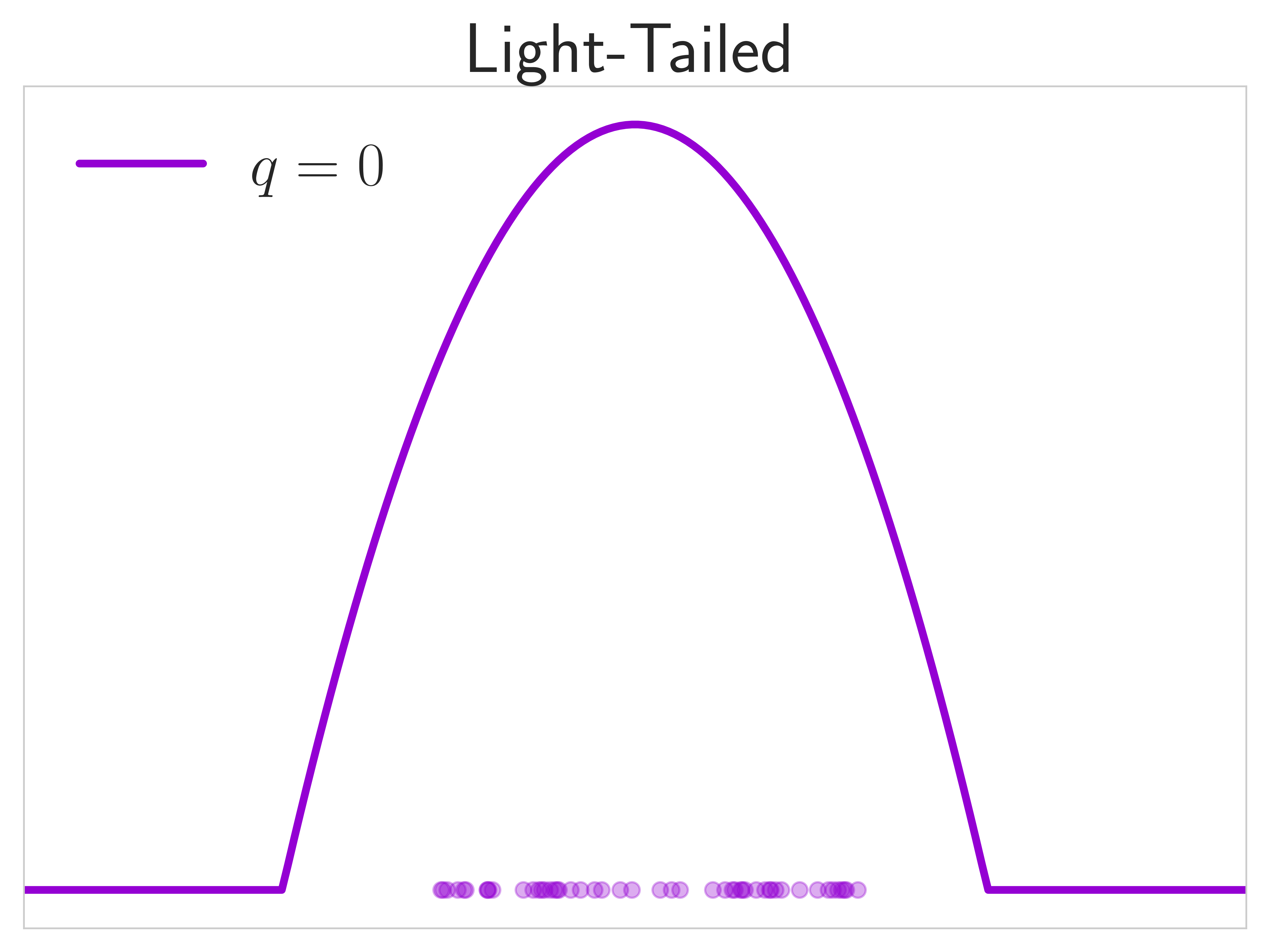
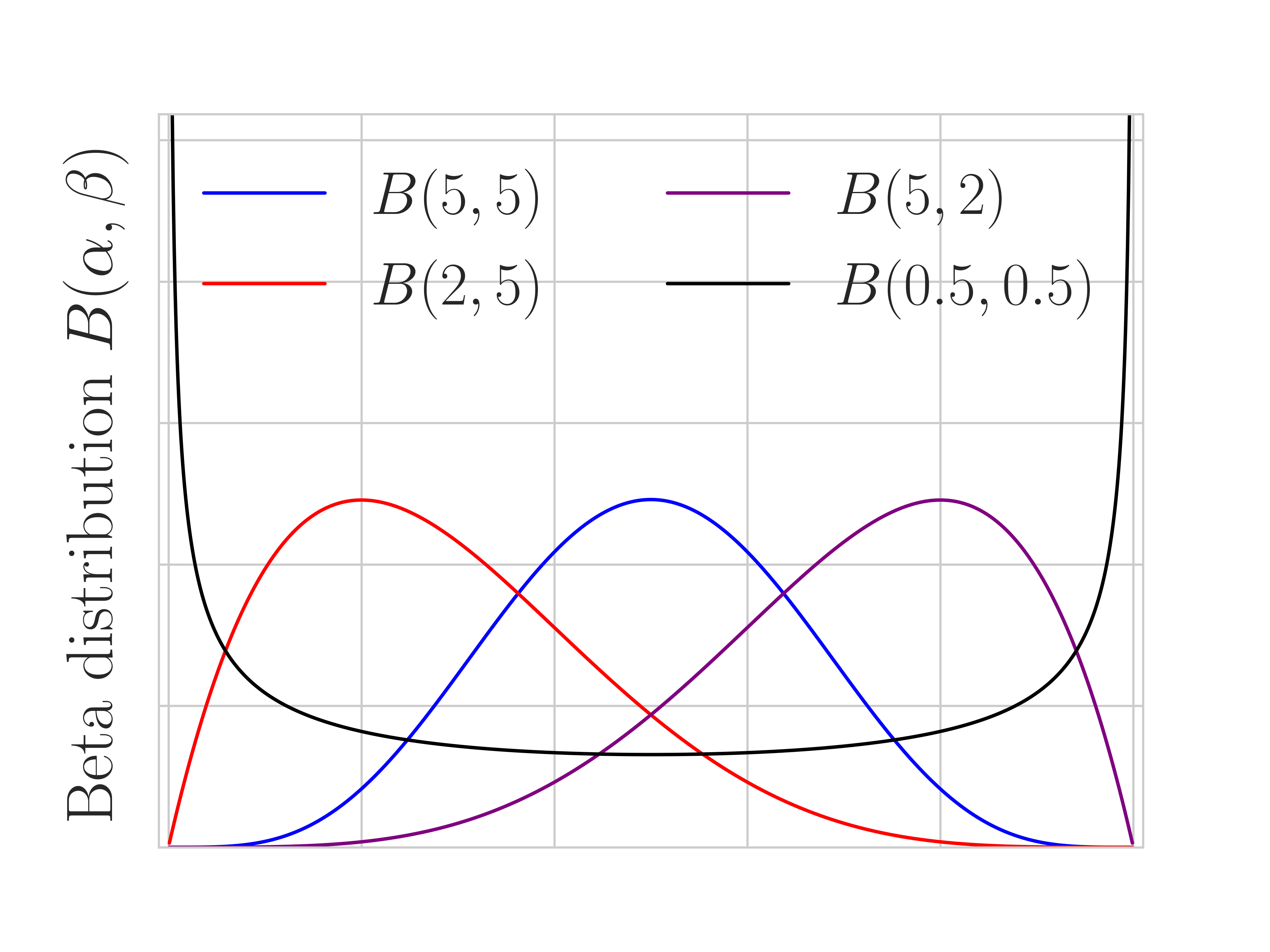
It is heavy-tailed when and light-tailed when . The condition is because is no longer integrable for (Naudts, 2010). We show in Figure 1 various -exponential policies. In Appendix A we provide a summary of multivariate densities introduced so far. It is worth noting that for -Gaussian a diagonal no longer leads to a product of independent univariate -Gaussians (Martins et al., 2022). We discuss how to sample from a -Gaussian in Appendix B.2.
4 -Exponential Family Via The Tsallis Regularization
The -exp family provides a general class of stochastic policies. But perhaps more importantly, they can be derived as solutions to the maximum Tsallis entropy principle (Suyari and Tsukada, 2005; Furuichi, 2010), generalizing the maximum Shannon entropy principle (Jaynes, 1957; Grünwald and Dawid, 2004; Ziebart, 2010). We discuss both principles in Eq. (7).
4.1 Boltzmann-Gibbs Regularization
Consider a regularized policy as the solution to the following regularization problem:
| (7) |
where is a proper, lower semi-continuous, strictly convex function. We can absorb the regularization coefficient into by . It is a classic result that at the limit the unregularized optimal action is recovered: , i.e., that maximizes .
One of the most well-studied regularizers is the negative Shannon entropy , which leads to the Boltzmann-Gibbs policy . Another popular choice is the KL divergence for some reference policy . The regularized policy is . Notice that it is also a member of the exponential family by writing .
4.2 Tsallis Regularization
Originally, the deformed logarithm function was introduced in the statistical physics to generalize the Shannon entropy by deforming the logarithm contained in it (Naudts, 2010). Consider replacing Shannon entropy in Eq.(7) with the negative Tsallis entropy . It has been shown that leads to following regularized policy:
| (8) |
We see that when , it recovers the sparsemax policy introduced in Section 3.2. As indicated by (Zhu et al., 2023), the effect of different lies in the extent of thresholding. One can also consider regularization by the Tsallis KL divergence (Furuichi et al., 2004). Likewise to the KL case, is typically taken to be the last policy, in which the regularized policy is the product of two -exp functions.
It is worth noting that there are other regularization functionals that can induce -exp policies. One of the prominent examples is the -entropy/divergence, which can be defined by simply letting in (Peters et al., 2019; Belousov and Peters, 2019). It is shown in (Xu et al., 2022, 2023) that when it induces the sparsemax policy. Therefore, -exp policies can also be viewed as solutions to the regularization.
4.3 Tsallis Advantage Weighted Actor Critic
An advantage of -exp (resp. exp) policies is it may improve the consistency of algorithms that explicitly mimics a -exp (resp. exp) policy. For example, Tsallis Advantage Weighted Actor Critic (TAWAC) proposed to use a light-tailed -exp policy for offline learning (Zhu et al., 2024). However, TAWAC was implemented with Gaussian, which amounts to approximating a light-tailed distribution using one with infinite support. Let denote the empirical behavior policy and the offline dataset. TAWAC minimizes the following actor loss, where we ignore the parametrization of value functions:
| (9) | ||||
where denotes the Tsallis KL regularized policy. We can generalize TAWAC to online learning by simply changing the expectation to be w.r.t. arbitrary behavior policy. It is clear that depending on , choosing Gaussian as may incur inconsistency with the theory. A -exp policy would be more suitable and could improve the performance. As evidenced by our experimental results, heavy tailed policies indeed further improve the performance of TAWAC by a large margin.
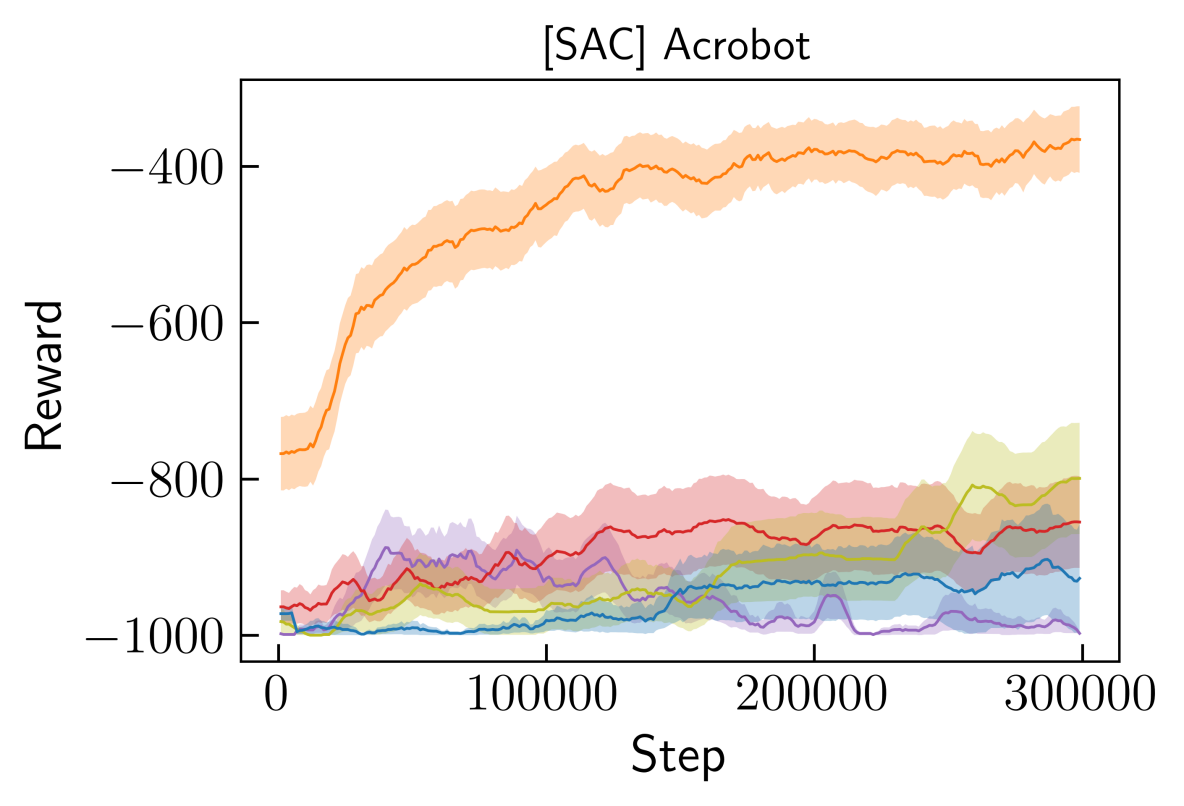
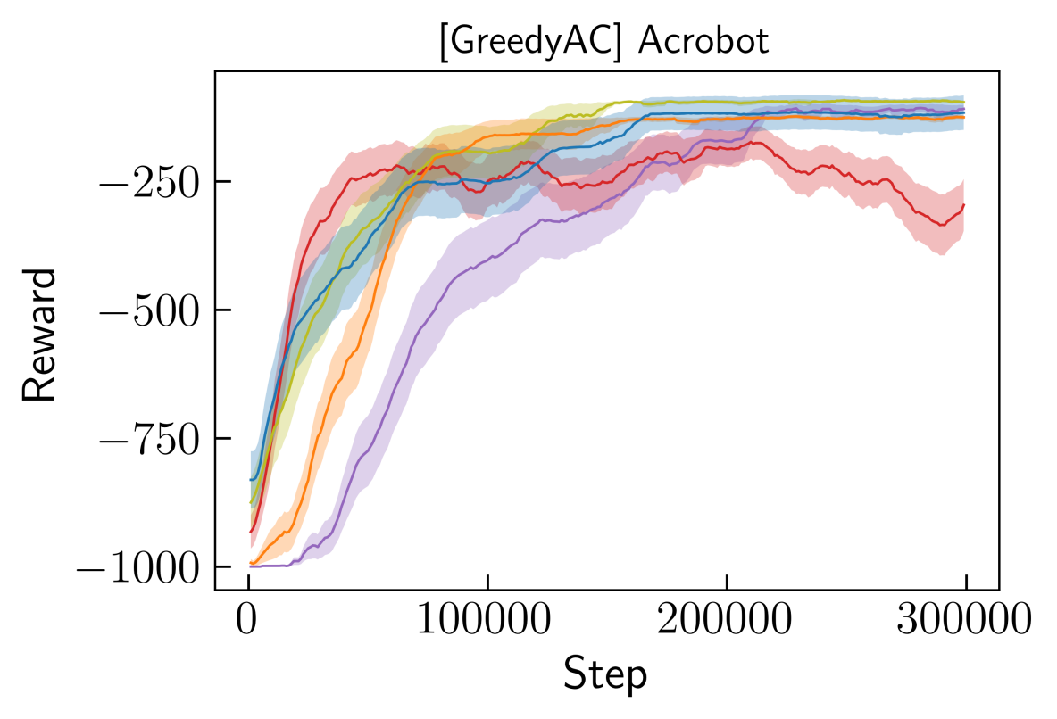
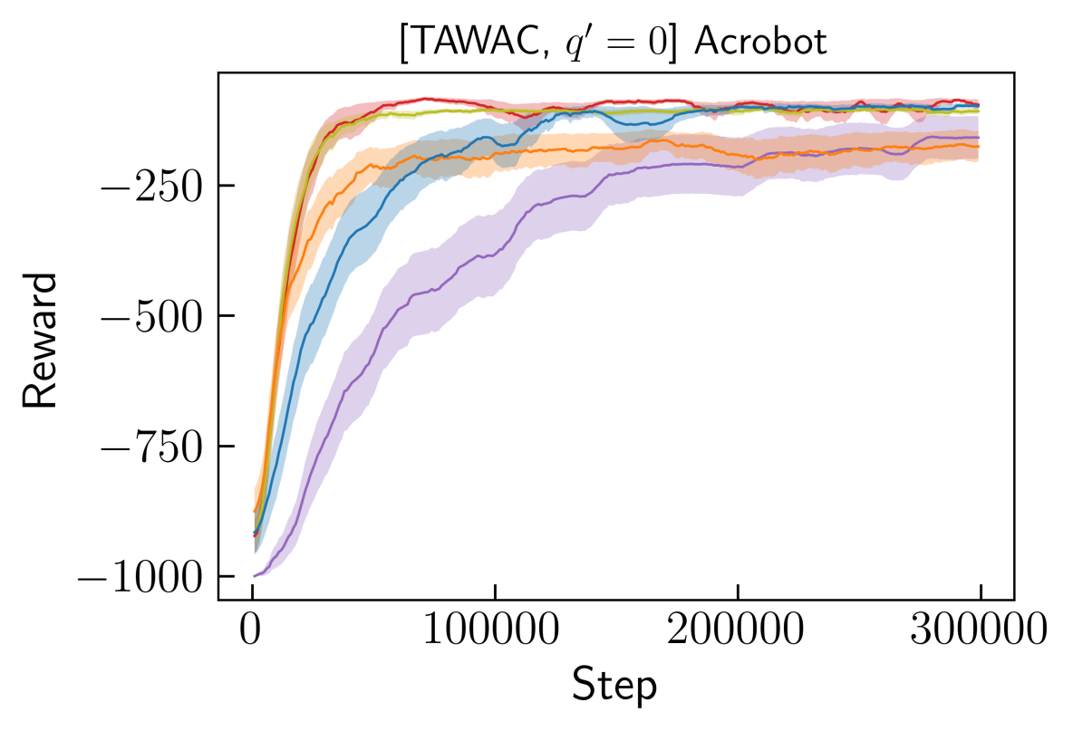
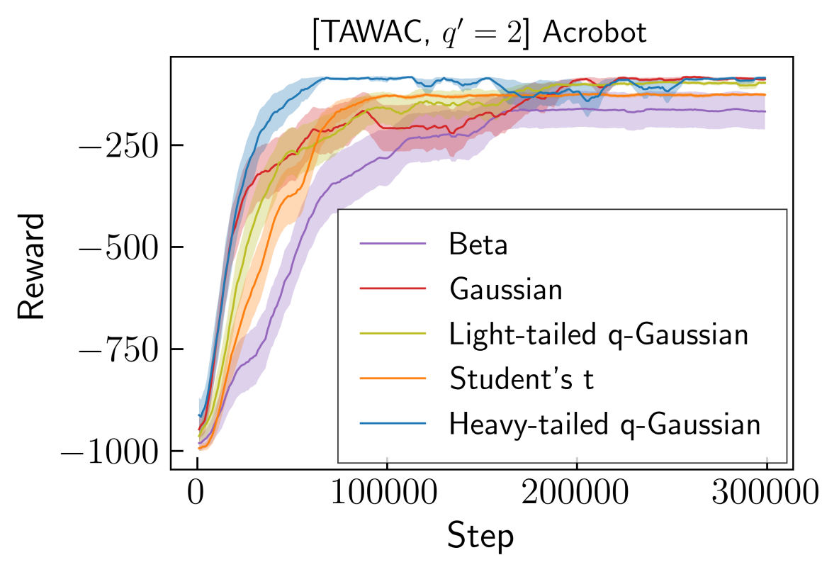
5 Experiments
Policy functional is typically a design choice regardless of online and offline problems. We are interested in the following questions: (i) is Gaussian policy, as the standard choice, necessarily superior? (ii) are algorithms sensitive to the choice of policy? (iii) when are the -exp policies useful? We seek to answer these questions by examining the combinations of policies plus various actor-critic methods on both online and offline problems.
We parametrize Student-t’s DOF parameter in addition to its location and scale. By contrast, the heavy-tailed -Gaussian is fixed at , since its allowable range is . For the light-tailed -Gaussian, we opt for the standard choice . For the light-tailed -Gaussian, numerical issues may be encountered when evaluating log-probabilities of off-policy actions. Whenever this happens, we replace them with on-policy samples with the smallest distance, see Appendix B.2 for detail.
5.1 Online Reinforcement Learning
Domains and Baselines. We used three classical control environments in the continuous action setting: Mountain Car (Sutton and Barto, 2018), Pendulum (Degris et al., 2012) and Acrobot (Sutton and Barto, 2018). We are using the cost-to-goal version of Mountain Car, which outputs reward per time step to encourage reaching the goal early. All environments truncate the episodes at 1000 time steps and use a discount factor of . Additional details on the environments, the experimental setup and hyper-parameter sweeps are provided in the Appendix B.2.2. To investigate what policies are preferred by what algorithms, we opt for the following algorithms: Soft Actor-Critic (SAC) (Haarnoja et al., 2018), Greedy Actor-Critic (GreedyAC) (Neumann et al., 2023) and the online version of Tsallis AWAC (TAWAC) (Zhu et al., 2024). These three algorithms can be seen to respectively implement Boltzmann-Gibbs regularization, no regularization, and Tsallis regularization, see Appendix C.1.
Results. Figure 2 shows the learning curves of all combinations on Acrobot. See Appendix D.1 for full environments. Several interesting observations can be drawn. For SAC: (1) while SAC + Gaussian is standard, it fails to learn anything without a sufficiently large entropy bonus () in this exploration-demanding environment. Such large entropy coefficients are unusual and we did not include them in the swept range; (2) Student’s t is the only learning policy with SAC. This suggests that Student’s t with adaptive DOF has strong exploration ability.
For GreedyAC, all policies converge to roughly the same level except Gaussian. This can be due to the fact that the Gaussian converges too quickly and no sufficient diverse samples can be produced by the proposal policy to update the actor towards the optimal region. To testify to this point, we visualize the evolution of policies in Figure 5 Left. Notice also that the superior performance of light-tailed -Gaussian validates our method for handling out-of-support actions.
TAWAC provides a means to examine consistency between the actor loss and policy. When , TAWAC minimizes KL loss to a light-tailed -exp policy. It can be seen that indeed the light-tailed -Gaussian quickly converges to the optimal score, and Gaussian performs equally well in this case. When , heavy-tailed -Gaussian can learn much quicker than other policies, though they finally converge to roughly the same level. These observations verified our analysis in Section 4.3.
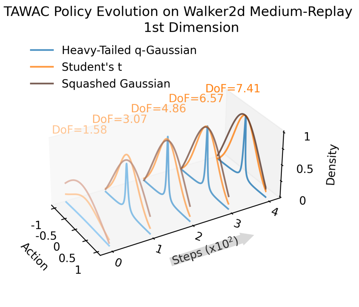
In Figure 5 Right we visualize the evolution of Gaussian and -Gaussian policies on the starting state over the first steps ( of the entire learning horizon). Note that the allowed action range is but the plot shows for better visualization. As stated, Gaussian tends to quickly concentrate like a delta policy. This can be detrimental to algorithms like SAC and GreedyAC which demand stochasticity to generate diverse samples. By contrast, both light- and heavy-tailed -Gaussians tend to be more stochastic.
5.2 Offline Reinforcement Learning
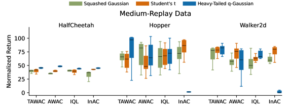

Domains and Baselines. We use the standard benchmark Mujoco suite from D4RL to evaluate algorithm-policy combinations (Fu et al., 2020). The following algorithms are compared: TAWAC, Advantage Weighetd Actor-Critic (AWAC) (Nair et al., 2021), Implicit Q-Learning (IQL) (Kostrikov et al., 2022), In-sample Actor-Critic (InAC) (Xiao et al., 2023). For TAWAC, we fix its leading -exp with . In Appendix C.2 we detail the compared algorithms. We also include a popular variant of Gaussian known as the Squashed Gaussian for comparison. Being able to evaluate the offline log-probability is critical to the tested algorithms, we find that light-tailed -Gaussian leads to poor performance even with random online sampling, hence we do not show them here.
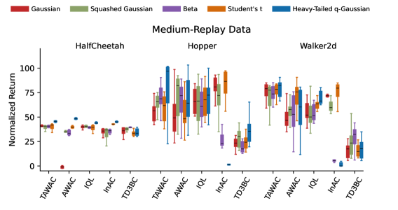
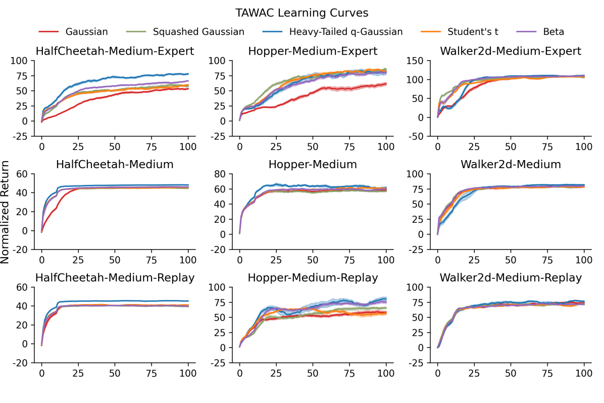
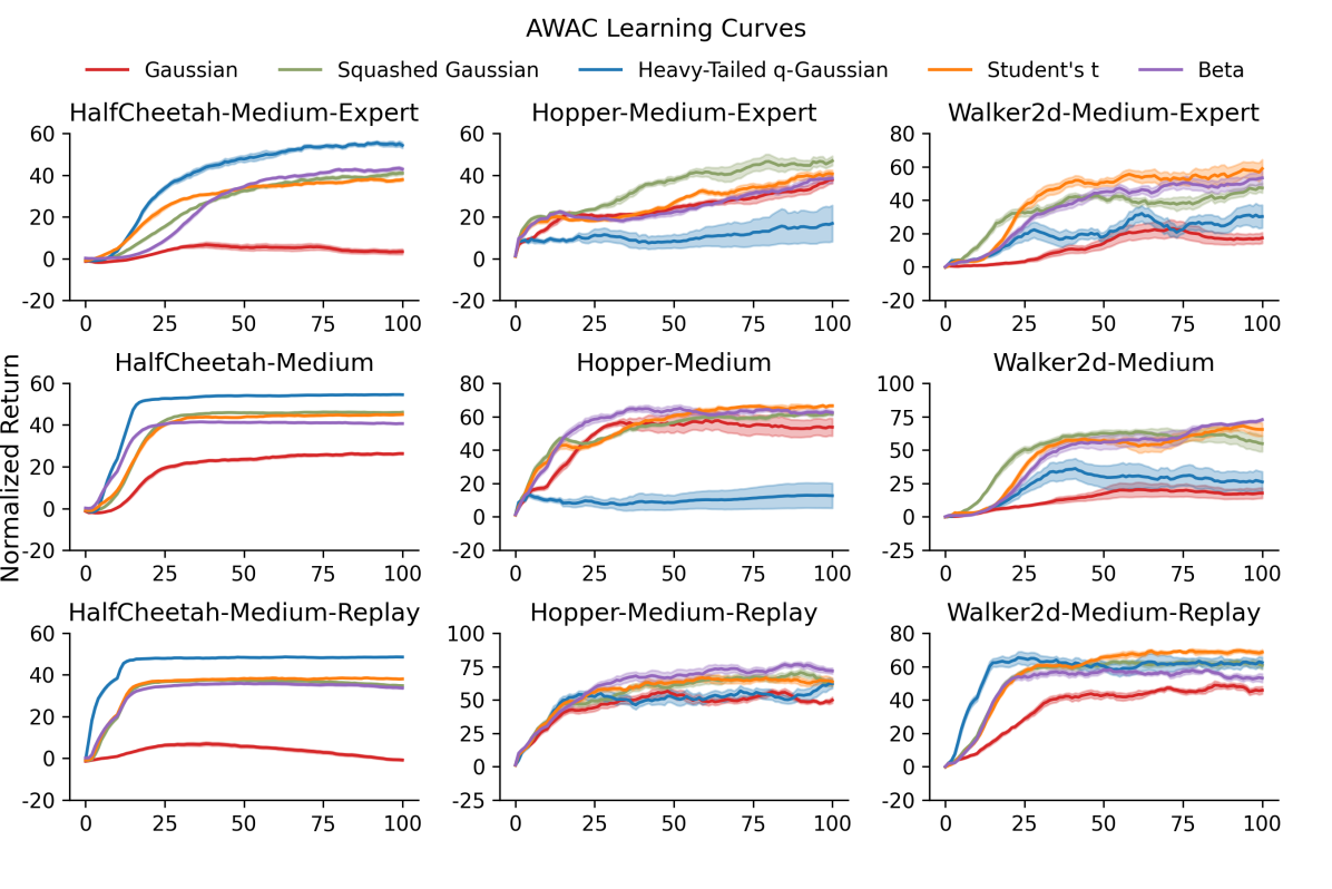
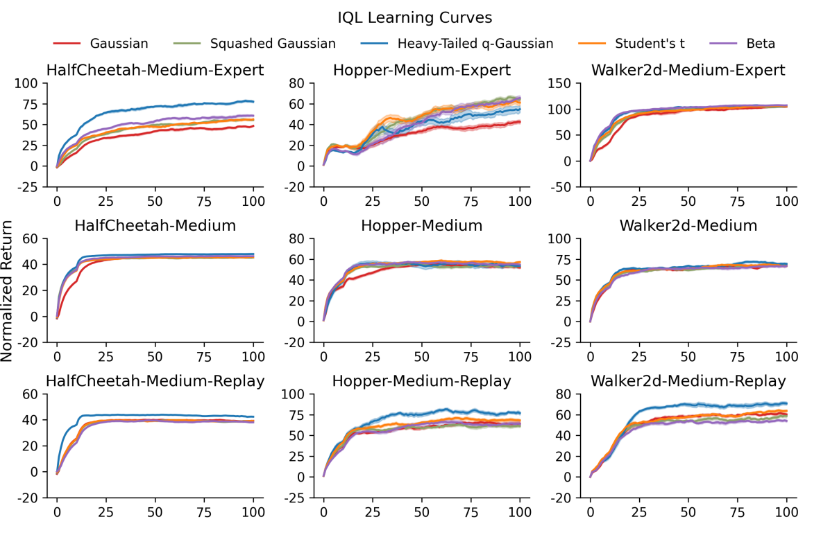
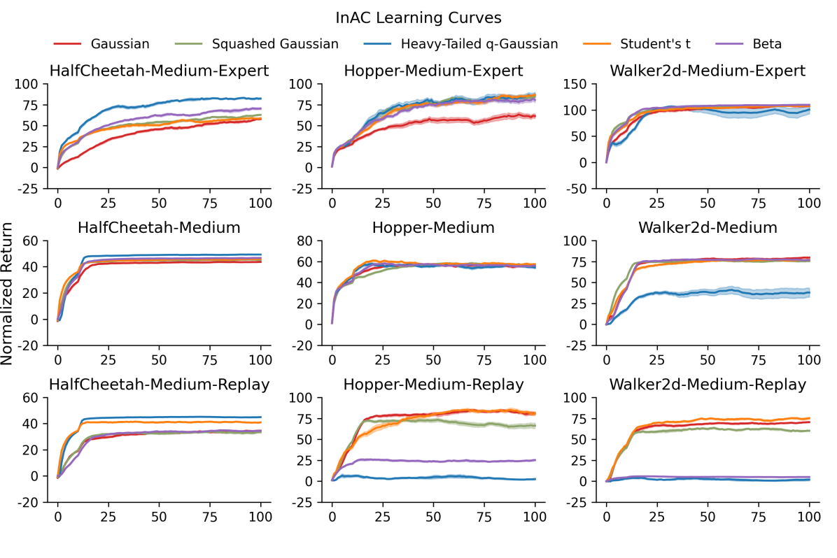
Results. Figure 3 compares the normalized scores on the Medium-Replay datasets. It can be seen that environment-wise, TAWAC + heavy-tailed -Gaussian is the top performer, and can improve on the Squashed Gaussian by a non-negligible margin. On HalfCheetah, heavy-tailed -Gaussian achieves the best score with every algorithm. Algorithm-wise, heavy-tailed -Gaussian or/and Student’s t are better or equivalent to the Squashed Gaussian, except with AWAC on Hopper. Student’s t is stable across algorithms, including these with which heavy-tailed -Gaussian performs poorly (e.g., InAC). This demonstrates the value of the learnable DOF parameter that allows it interpolates Gaussian. In Appendix D.2 we provide comparison on other policies and datasets.
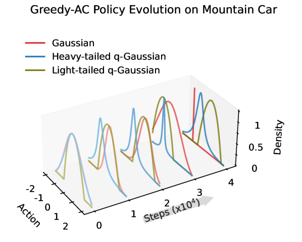

Figure 4 summarizes the relative improvement over the Squashed Gaussian across environments. Several observations can be made: (i) though Squashed Gaussian improves upon Gaussian in general, it is seldom the best performer. (ii) heavy-tailed -Gaussian and Student’s t can consistently improve the performance, sometimes by . (iii) though there is no single policy performing the best for all cases, choosing Heavy-tailed -Gaussian for -exp based actors (e.g. TAWAC), and Student’s t for exp-based actors (AWAC, IQL, InAC) are generally effective.
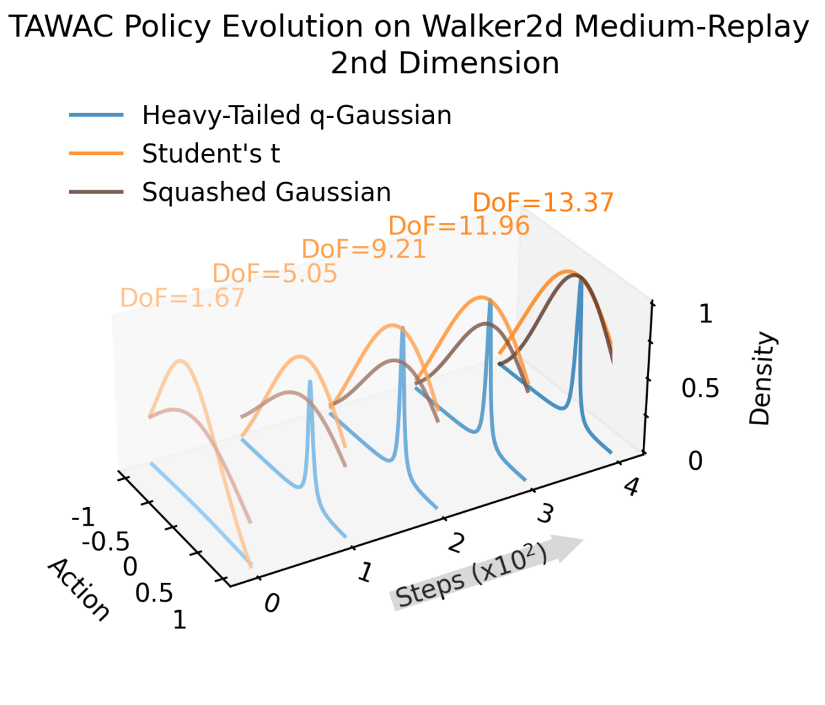
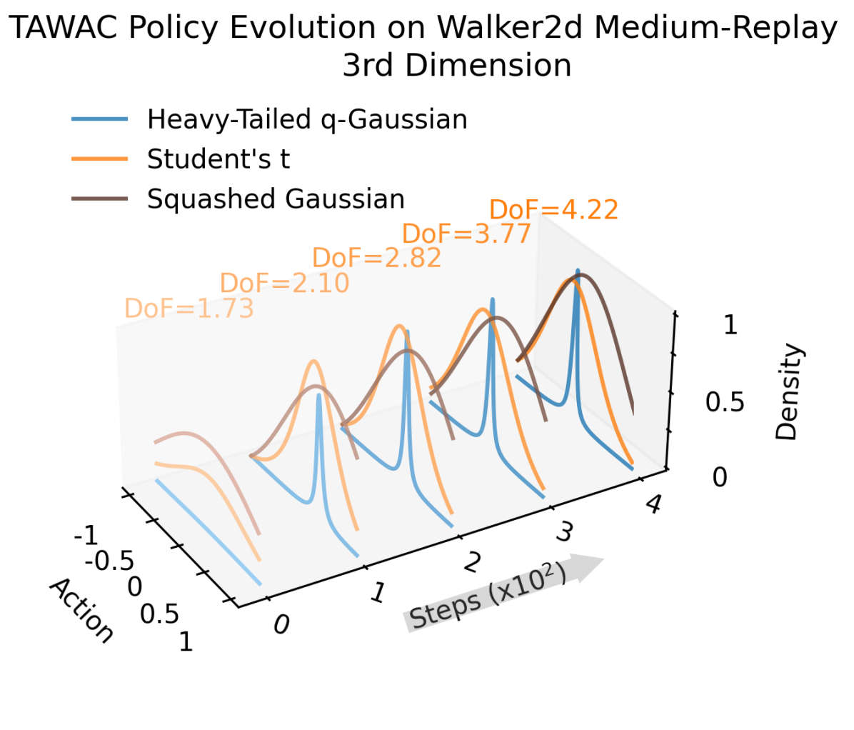
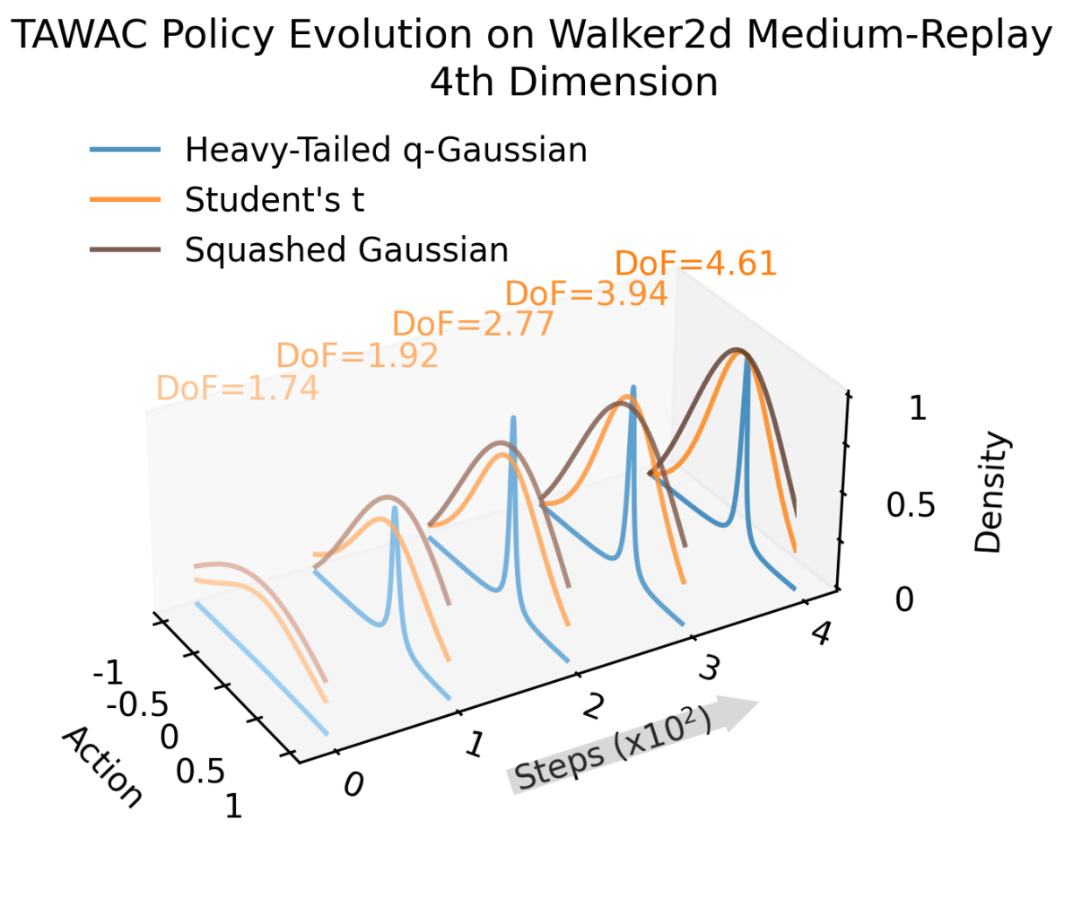
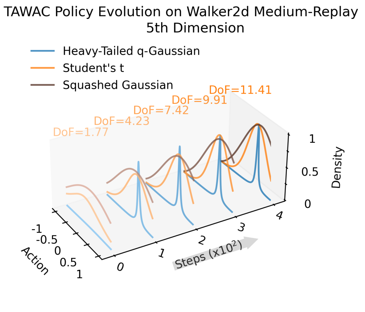
Figure 5 right visualizes the policy evolution of Squashed Gaussian and the two heavy-tailed policies, learned with TAWAC on Medium-Replay Walker2D. Squashed Gaussian tends to converge slower here. Since the offline Mujoco environments are fully deterministic, a wide distribution indicates failure of finding the mode of the optimal action and therefore can be detrimental to learning performance. In Figure 14 we show all action dimensions. Student’s t is flexible in that it can imitate Gaussian by having large DOF on some dimensions and take on a narrower shape on the other.
6 Conclusion
Gaussian policy is standard for RL algorithms on continuous action spaces. In this paper we considered a broader family of policies that remains tractable, called the -exponential family. We focused on location-scale members in the -exp family. Specifically, we looked at Student’s t, light- and heavy-tailed -Gaussian policies. Actor-critic methods that mimic regularized policies (e.g. KL-regularized) may result in preference over some specific choice of policy. Extensive experiments on both online and offline tasks with various actor-critic methods showed that heavy-tailed policies are in general effective. In particular, we found the Student’s t policy to be more stable than Gaussian across settings thanks to its learnable degree of freedom parameter. Heavy-tailed -Gaussian performed favorably with Tsallis Advantage Weighted Actor-Critic in offline benchmark problems.
We acknowledge that the paper has limitations. Perhaps the greatest is the inherent dilemma of the light-tailed -Gaussian evaluating out-of-support actions. Off-policy/offline algorithms require evaluating actions from some behavior policy and they can be out of the support of the current -Gaussian. Naïvely discarding these samples results extremely slow or no learning. In this paper we proposed to alleviate this issue by using on-policy samples with the smallest distance. Nonetheless, it did not help in offline experiments. There are two potential solutions: the first is to project out-of-support actions precisely to the boundary of the -Gaussian; the second is to initialize the policy with sufficiently large scale and anneal it slowly. We leave them to future investigations.
References
- Ahmed et al. [2019] Z. Ahmed, N. Le Roux, M. Norouzi, and D. Schuurmans. Understanding the impact of entropy on policy optimization. In Proceedings of 36th International Conference on Machine Learning, volume 97, pages 151–160, 2019.
- Amari and Ohara [2011] S.-i. Amari and A. Ohara. Geometry of q-exponential family of probability distributions. Entropy, 13(6):1170–1185, 2011.
- Amid et al. [2019] E. Amid, M. K. Warmuth, and S. Srinivasan. Two-temperature logistic regression based on the tsallis divergence. In Proceedings of the Twenty-Second International Conference on Artificial Intelligence and Statistics, volume 89, pages 2388–2396, 2019.
- Bartumeus et al. [2005] F. Bartumeus, M. G. E. da Luz, G. M. Viswanathan, and J. Catalan. Animal search strategies: A quantitative random-walk analysis. Ecology, 86(11):3078–3087, 2005.
- Belousov and Peters [2019] B. Belousov and J. Peters. Entropic regularization of markov decision processes. Entropy, 21(7), 2019.
- Cen et al. [2022] S. Cen, C. Cheng, Y. Chen, Y. Wei, and Y. Chi. Fast global convergence of natural policy gradient methods with entropy regularization. Operations Research, 70(4):2563–2578, 2022.
- Chou et al. [2017] P.-W. Chou, D. Maturana, and S. Scherer. Improving stochastic policy gradients in continuous control with deep reinforcement learning using the beta distribution. In Proceedings of the 34th International Conference on Machine Learning, pages 834–843, 2017.
- Chow et al. [2018] Y. Chow, O. Nachum, and M. Ghavamzadeh. Path consistency learning in Tsallis entropy regularized MDPs. In International Conference on Machine Learning, pages 979–988, 2018.
- Cover and Thomas [2006] T. M. Cover and J. A. Thomas. Elements of Information Theory (Wiley Series in Telecommunications and Signal Processing). Wiley-Interscience, USA, 2006.
- Degris et al. [2012] T. Degris, M. White, and R. S. Sutton. Off-policy actor-critic. In Proceedings of the 29th International Coference on International Conference on Machine Learning, page 179–186, 2012.
- Ding and Vishwanathan [2010] N. Ding and S. Vishwanathan. t-logistic regression. In Advances in Neural Information Processing Systems, volume 23, 2010.
- Fu et al. [2020] J. Fu, A. Kumar, O. Nachum, G. Tucker, and S. Levine. D4rl: Datasets for deep data-driven reinforcement learning, 2020.
- Fujimoto and Gu [2021] S. Fujimoto and S. S. Gu. A minimalist approach to offline reinforcement learning. In Thirty-Fifth Conference on Neural Information Processing Systems, 2021.
- Furuichi [2010] S. Furuichi. On the maximum entropy principle and the minimization of the fisher information in tsallis statistics. Journal of Mathematical Physics, 50:013303, 01 2010.
- Furuichi et al. [2004] S. Furuichi, K. Yanagi, and K. Kuriyama. Fundamental properties of tsallis relative entropy. Journal of Mathematical Physics, 45(12):4868–4877, 2004.
- Garg et al. [2023] D. Garg, J. Hejna, M. Geist, and S. Ermon. Extreme q-learning: Maxent RL without entropy. In The Eleventh International Conference on Learning Representations, 2023.
- Grünwald and Dawid [2004] P. Grünwald and A. Dawid. Game theory, maximum entropy, minimum discrepancy and robust bayesian decision theory. Annals of Statistics, 32, 2004.
- Gu et al. [2016] S. Gu, T. Lillicrap, I. Sutskever, and S. Levine. Continuous deep q-learning with model-based acceleration. In Proceedings of The 33rd International Conference on Machine Learning, pages 2829–2838, 2016.
- Haarnoja et al. [2018] T. Haarnoja, A. Zhou, P. Abbeel, and S. Levine. Soft actor-critic: Off-policy maximum entropy deep reinforcement learning with a stochastic actor. In Proceedings of the 35th International Conference on Machine Learning, pages 1861–1870, 2018.
- Jaynes [1957] E. T. Jaynes. Information theory and statistical mechanics. Phys. Rev., 106:620–630, 1957.
- Kobayashi [2019] T. Kobayashi. Student-t policy in reinforcement learning to acquire global optimum of robot control. Applied Intelligence, 49:4335–4347, 2019.
- Kostrikov et al. [2022] I. Kostrikov, A. Nair, and S. Levine. Offline reinforcement learning with implicit q-learning. In International Conference on Learning Representations, 2022.
- Lange et al. [1989] K. L. Lange, R. J. A. Little, and J. M. G. Taylor. Robust statistical modeling using the t distribution. Journal of the American Statistical Association, 84:881–896, 1989.
- Lee et al. [2018] K. Lee, S. Choi, and S. Oh. Sparse markov decision processes with causal sparse tsallis entropy regularization for reinforcement learning. IEEE Robotics and Automation Letters, 3:1466–1473, 2018.
- Lee et al. [2020] K. Lee, S. Kim, S. Lim, S. Choi, M. Hong, J. I. Kim, Y. Park, and S. Oh. Generalized tsallis entropy reinforcement learning and its application to soft mobile robots. In Robotics: Science and Systems XVI, pages 1–10, 2020.
- Li et al. [2023] Y. Li, W. Zhou, and R. Zhu. Quasi-optimal reinforcement learning with continuous actions. In The Eleventh International Conference on Learning Representations, 2023.
- Martins and Astudillo [2016] A. F. T. Martins and R. F. Astudillo. From softmax to sparsemax: A sparse model of attention and multi-label classification. In Proceedings of the 33rd International Conference on Machine Learning, page 1614–1623, 2016.
- Martins et al. [2022] A. F. T. Martins, M. Treviso, A. Farinhas, P. M. Q. Aguiar, M. A. T. Figueiredo, M. Blondel, and V. Niculae. Sparse continuous distributions and fenchel-young losses. Journal of Machine Learning Research, 23(257):1–74, 2022.
- Matsuzoe and Ohara [2011] H. Matsuzoe and A. Ohara. Geometry of q-exponential families. In Recent Progress in Differential Geometry and Its Related Fields, pages 55–71, 2011.
- Mei et al. [2020] J. Mei, C. Xiao, C. Szepesvari, and D. Schuurmans. On the global convergence rates of softmax policy gradient methods. In Proceedings of the 37th International Conference on Machine Learning, volume 119, pages 6820–6829, 2020.
- Nair et al. [2021] A. Nair, M. Dalal, A. Gupta, and S. Levine. {AWAC}: Accelerating online reinforcement learning with offline datasets, 2021.
- Naudts [2002] J. Naudts. Deformed exponentials and logarithms in generalized thermostatistics. Physica A-statistical Mechanics and Its Applications, 316:323–334, 2002.
- Naudts [2010] J. Naudts. The q-exponential family in statistical physics. Journal of Physics: Conference Series, page 012003, 2010.
- Neumann et al. [2023] S. Neumann, S. Lim, A. G. Joseph, Y. Pan, A. White, and M. White. Greedy actor-critic: A new conditional cross-entropy method for policy improvement. In The Eleventh International Conference on Learning Representations, 2023.
- Paszke et al. [2019] A. Paszke, S. Gross, F. Massa, A. Lerer, J. Bradbury, G. Chanan, T. Killeen, Z. Lin, N. Gimelshein, L. Antiga, A. Desmaison, A. Kopf, E. Yang, Z. DeVito, M. Raison, A. Tejani, S. Chilamkurthy, B. Steiner, L. Fang, J. Bai, and S. Chintala. Pytorch: An imperative style, high-performance deep learning library. In Advances in Neural Information Processing Systems 32, pages 8024–8035, 2019.
- Peters et al. [2019] B. Peters, V. Niculae, and A. F. T. Martins. Sparse sequence-to-sequence models. In Proceedings of the 57th Annual Meeting of the Association for Computational Linguistics, pages 1504–1519, 2019.
- Petersen and Pedersen [2012] K. B. Petersen and M. S. Pedersen. The matrix cookbook. 2012.
- Sears [2008] T. Sears. Generalized Maximum Entropy, Convexity and Machine Learning. PhD thesis, The Australian National University and Computer Science Laboratory, Research School of Information Sciences and Engineering, 2008.
- Sutton and Barto [2018] R. S. Sutton and A. G. Barto. Reinforcement Learning: An Introduction. A Bradford Book, Cambridge, MA, USA, 2018.
- Sutton et al. [1999] R. S. Sutton, D. McAllester, S. Singh, and Y. Mansour. Policy gradient methods for reinforcement learning with function approximation. In Advances in Neural Information Processing Systems (NIPS), pages 1057–1063, 1999.
- Suyari and Tsukada [2005] H. Suyari and M. Tsukada. Law of error in tsallis statistics. IEEE Transactions on Information Theory, 51(2):753–757, 2005.
- Thistleton et al. [2007] W. J. Thistleton, J. A. Marsh, K. Nelson, and C. Tsallis. Generalized box–mÜller method for generating -gaussian random deviates. IEEE Transactions on Information Theory, 53:4805–4810, 2007.
- Tsallis [2009] C. Tsallis. Introduction to Nonextensive Statistical Mechanics: Approaching a Complex World. Springer New York, 2009. ISBN 9780387853581.
- Vieillard et al. [2020] N. Vieillard, T. Kozuno, B. Scherrer, O. Pietquin, R. Munos, and M. Geist. Leverage the average: an analysis of regularization in rl. In Advances in Neural Information Processing Systems 33, pages 1–12, 2020.
- Xiao et al. [2023] C. Xiao, H. Wang, Y. Pan, A. White, and M. White. The in-sample softmax for offline reinforcement learning. In The Eleventh International Conference on Learning Representations, 2023.
- Xu et al. [2022] H. Xu, L. Jiang, J. Li, and X. Zhan. A policy-guided imitation approach for offline reinforcement learning. In A. H. Oh, A. Agarwal, D. Belgrave, and K. Cho, editors, Advances in Neural Information Processing Systems, 2022.
- Xu et al. [2023] H. Xu, L. Jiang, J. Li, Z. Yang, Z. Wang, V. W. K. Chan, and X. Zhan. Offline RL with no OOD actions: In-sample learning via implicit value regularization. In The Eleventh International Conference on Learning Representations, 2023.
- Zhu et al. [2023] L. Zhu, Z. Chen, M. Schlegel, and M. White. Generalized munchausen reinforcement learning using tsallis kl divergence. In Advances in Neural Information Processing Systems (NeurIPS), 2023.
- Zhu et al. [2024] L. Zhu, M. Schlegel, H. Wang, and M. White. Offline reinforcement learning with tsallis regularization. Transactions on Machine Learning Research, 2024.
- Ziebart [2010] B. D. Ziebart. Modeling Purposeful Adaptive Behavior with the Principle of Maximum Causal Entropy. PhD thesis, Carnegie Mellon University, 2010.
Appendix
The Appendix is organized into the following sections. In section A we summarize the multivariate form of -exp policies and derive gradients of their log-likelihood. We then provide implementation details including hyperparameters and how to sample from -Gaussian in section B. In section C we discuss how different algorithms may prefer specific policies depending on its actor loss. Lastly we provide additional experimental results in section D.
- A
- B
- C
- D
Appendix A Multivariate Density of -exp Policies
In Table 3 we show multivariate density of the -exp policies introduced in the main text. Note that multivariate Student’s t is constructed based on the assumption that a diagonal leads to independent action dimensions, same as the Gaussian policy. On the other hand, for -Gaussian this is no longer true, since a diagonal does not lead to product of univariate densities.
In the main text we showed their one-dimensional cases for simplicity. For experiments the multivariate densities were used for experiments. We now derive their gradients of log-likelihood with respect to parameters. The following equations will be used frequently [Petersen and Pedersen, 2012]:
| (10) | |||
| (11) | |||
| (12) |
With these tools in hand, the following gradient expressions can be readily derived.
A.1 Gaussian
A.2 Student’s t
A.3 -Gaussian
Since we do not parametrize the entropic index , the gradients of log-likelihood with respect to are the same for both heavy- and light-tailed -Gaussian. Therefore, we focus on the light-tailed case and absorb into the constant the terms only related to .
| (15) | ||||
It is interesting to see that the gradients of -Gaussian log-likelihood can be seen as the Gaussian counterparts scaled by the reciprocal of . Since can take on zero values when , the gradients as well as the log-likelihood function may be undefined outside the support. However, this does not happen for heavy-tailed -Gaussian .
To make these policies suitable for deep reinforcement learning, we discuss in Appendix B how to parametrize the policies using neural networks.
Appendix B Implementation Details
Details of our implementation is provided in this section. Specifically, we detail our design choices and provide code examples on how to parametrize the policies using neural networks. Since -Gaussian is not yet supported in popular libraries like PyTorch [Paszke et al., 2019], we also discuss how to efficiently sample from a -Gaussian.
B.1 Sampling from -Gaussian
We discuss how to sample from -Gaussian in this section. Specifically, we mention the stochastic representation (or reparametrization) by [Martins et al., 2022] to sample from a light-tailed (<1) -Gaussian distributions and the Generalized Box-Müller Method (GBMM) [Thistleton et al., 2007] to sample general -Gaussian variables.
B.1.1 Stochastic Representation
It was shown by [Martins et al., 2022] that a light-tailed -Gaussian with permits a stochastic representation , where is a random sample from the -dimensional unit sphere. is the scaled matrix . is the radius of the distribution, and the ratio follows the Beta distribution:
where is radius of the supporting sphere of the standard -Gaussian :
Since the radius depends only on the dimensionality and the entropic index , we can compute the desired radius by first sampling from then multiplied by . The reader is referred to [Martins et al., 2022] for more details.
B.1.2 Generalized Box-Müller Method
The reparametrization method in [Martins et al., 2022, Proposition 16] relies on bounded radius . It is not straightforward to generalize their proof to the unbounded case which corresponds to heavy-tailed distributions. Fortunately, we can rely on the Generalized Box-Müller Method to map uniform random variables to -Gaussian variables for all [Thistleton et al., 2007]. Specifically, we sample and compute the following:
then each of is a standard -Gaussian with new entropic index . Often we know the desired in advance, in this case we simply generate variables by using . To sample from , we sample uniform random vectors and compute the transformed via GBMM. The desired random vector is given by . In Figure 6 we visualize densities and samples of both heavy-tailed and light-tailed -Gaussian. The densities were plotted using analytic expressions, and samples were drawn using GBMM. As discussed in [Thistleton et al., 2007], GBMM produces high-quality samples that concord well with their theoretical densities.
B.2 Implementation Details
Our implementation includes handling policy parametrizations and tune the algorithms accordingly. We first introduce how the introduced policies are parametrized.
B.2.1 Policies
We discuss how to parametrize Beta, Student’s t and -Gaussian policies. Specifically, we parametrize for Beta policy; for -Gaussian. In additional to location and scale, Student’s t has an additional learnable parameter .
For Student’s t policy, we initialized a base DOF and learn by the softplus function. The Student’s t policy therefore always has DOF , which is equivalent to starting as the Cauchy’s distribution. For Beta policy, we similarly constrain to be the output of softplus function plus 1. This is because when the Beta policy takes on a bowl shape rather than a bell shape, see Figure 7. For Gaussian and -Gaussian policies, we follow the standard practice to parametrize mean by the tanh activation and scale by the log-std transform.
In the tested off-policy/offline algorithms, it is necessary to evaluate log-probability for off-policy/offline actions stored in the buffer. For light-tailed -Gaussian this can cause numerical issues since the evaluated actions may fall outside the support, incurring for log-probability. To avoid this issue, we sample a batch of on-policy actions from the -Gaussian and replace the out-of-support actions with the nearest action in the sense.
B.2.2 Online Experiments
We used three classical control environments in the continuous action setting: Mountain Car [Sutton and Barto, 2018], Pendulum [Degris et al., 2012] and Acrobot [Sutton and Barto, 2018]. All episodes are truncated at 1000 time steps. In Mountain Car, the action is the force applied to the car in , and the agent receives a reward of -1 at every time step. In Pendulum, the action is the torque applied to the base of the pendulum in and the reward is defined by where denotes the angle, is the derivative of time and the torque applied. Finally, in acrobot, the action is the torque applied on the joint between two links in and the agent receives a reward of per time step.
Experiment settings: When sweeping different hyperparameter configurations, we pause the training every 10,000 time steps and then evaluate the learned policy by averaging the total reward over 3 episodes. However, when running the best hyperparameter configuration, we evaluate by freezing the policy every 1000 time steps and then computing the total reward obtained for 1 episode.
Parameter sweeping: We sweep the hyperparameters with 5 independent runs and then evaluate the run configuration for 30 seeds. We select the best hyperparameters based on the overall area under curve. When running the best hyperparameter configurations, we discard the original 5 seeds used for the hyperparameter sweep in order to avoid the bias caused by hyperparameter selection. Details regarding the fixed and swept hyperparameters are provided in Table 4.
Agent learning: We used a 2-layer network with 64 nodes on each layer and ReLU non-linearities. The batch size was 32. Agents used a target network for the critic, updated with polyak averaging with .
| Hyperparameter | Value |
| Critic Learning rate | Swept in |
| Critic learning rate multiplier for actor | Swept in |
| Temperature | Swept in |
| Discount rate | 0.99 |
| Hidden size of Value network | 64 |
| Hidden layers of Value network | 2 |
| Hidden size of Policy network | 64 |
| Hidden layers of Policy network | 2 |
| Minibatch size | 32 |
| Adam. | 0.9 |
| Adam. | 0.999 |
| Number of seeds for sweeping | 10 |
| Number of seeds for the best setting | 30 |
B.2.3 Offline Experiments
We use the Mujoco suite from D4RL (Apache-2/CC-BY licence) [Fu et al., 2020] for offline experiments. The offline datasets are collected by a SAC agent, and their naming reflects the level of the trained agent used to collect the transitions. the medium dataset contains 1 million samples generated by a partially-trained SAC policy. Medium-expert combines the trajectories of the expert and the medium. Medium-replay consists of samples in the replay buffer during training until the policy reaches the medium level of performance.
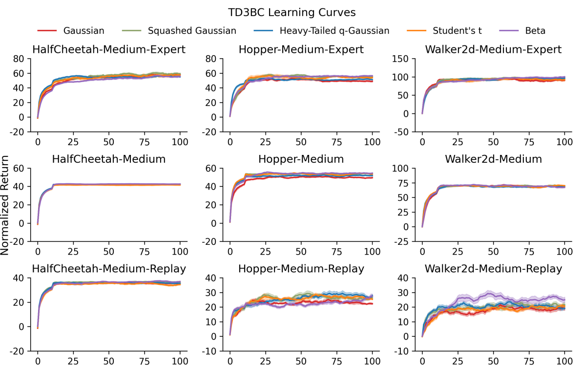
Experiment settings: We conducted the offline experiment using 9 datasets provided in D4RL: halfcheetah-medium-expert, halfcheetah-medium, halfcheetah-medium-replay, hopper-medium-expert, hopper-medium, hopper-medium-replay, walker2d-medium-expert, walker2d-medium, and walker2d-medium-replay. We run 5 agents: TAWAC, AWAC, IQL, InAC, and TD3BC. The results of TD3BC are posted in the appendix. For each agent, we tested 5 distributions: Gaussian, Squashed Gaussian, Beta, Student’s t, and Heavy-tailed -Gaussian. As offline learning algorithms usually require a distribution covering the whole action space, Light-tailed q-Gaussian is not considered in offline learning experiments. Each agent was trained for steps. The policy was evaluated every steps. The score was averaged over rollouts in the real environment; each had steps.
Parameter sweeping: All results shown in the paper were generated by the best parameter setting after sweeping. We list the parameter setting in Table 5. Learning rate and temperature in TAWAC + medium datasets were swept as the experiments in their publication did not include the medium dataset. The best learning rates are reported in Table 6, and the best temperatures for TAWAC + medium datasets are reported in Table 7.
| Hyperparameter | Value |
| Learning rate | Swept in See the best setting in Table 6 |
| Temperature | Same as the number reported in the publication of each algorithm. Except in TAWAC + medium datasets, the value was swept in . See the best setting in Table 7 |
| Discount rate | 0.99 |
| Hidden size of Value network | 256 |
| Hidden layers of Value network | 2 |
| Hidden size of Policy network | 256 |
| Hidden layers of Policy network | 2 |
| Minibatch size | 256 |
| Adam. | 0.9 |
| Adam. | 0.99 |
| Number of seeds for sweeping | 5 |
| Number of seeds for the best setting | 10 |
| Dataset | Distribution | TAWAC | AWAC | IQL | InAC | TD3BC |
| HalfCheetah-Medium-Expert | Heavy-Tailed q-Gaussian | 0.001 | 0.001 | 0.001 | 0.001 | 0.001 |
| HalfCheetah-Medium-Expert | Squashed Gaussian | 0.001 | 0.0003 | 0.0003 | 0.001 | 0.0003 |
| HalfCheetah-Medium-Expert | Gaussian | 0.0003 | 0.0001 | 0.0003 | 0.0003 | 0.0003 |
| HalfCheetah-Medium-Expert | Beta | 0.001 | 0.0003 | 0.001 | 0.001 | 0.0003 |
| HalfCheetah-Medium-Expert | Student’s t | 0.001 | 0.001 | 0.0003 | 0.001 | 0.0003 |
| HalfCheetah-Medium-Replay | Heavy-Tailed q-Gaussian | 0.001 | 0.001 | 0.001 | 0.001 | 0.003 |
| HalfCheetah-Medium-Replay | Squashed Gaussian | 0.001 | 0.0003 | 0.0003 | 0.001 | 0.003 |
| HalfCheetah-Medium-Replay | Gaussian | 0.001 | 0.0001 | 0.0003 | 0.001 | 0.001 |
| HalfCheetah-Medium-Replay | Beta | 0.001 | 0.0003 | 0.0003 | 0.001 | 0.001 |
| HalfCheetah-Medium-Replay | Student’s t | 0.001 | 0.0003 | 0.0003 | 0.001 | 0.0003 |
| HalfCheetah-Medium | Heavy-Tailed q-Gaussian | 0.001 | 0.001 | 0.001 | 0.001 | 0.001 |
| HalfCheetah-Medium | Squashed Gaussian | 0.001 | 0.0003 | 0.001 | 0.001 | 0.0003 |
| HalfCheetah-Medium | Gaussian | 0.0003 | 0.0001 | 0.0003 | 0.001 | 0.001 |
| HalfCheetah-Medium | Beta | 0.001 | 0.001 | 0.001 | 0.001 | 0.0003 |
| HalfCheetah-Medium | Student’s t | 0.001 | 0.0003 | 0.001 | 0.001 | 0.0003 |
| Hopper-Medium-Expert | Heavy-Tailed q-Gaussian | 0.001 | 0.0003 | 0.001 | 0.001 | 0.001 |
| Hopper-Medium-Expert | Squashed Gaussian | 0.001 | 0.001 | 0.001 | 0.001 | 0.0001 |
| Hopper-Medium-Expert | Gaussian | 0.0003 | 0.0003 | 0.001 | 0.001 | 0.0001 |
| Hopper-Medium-Expert | Beta | 0.001 | 0.001 | 0.001 | 0.003 | 0.0003 |
| Hopper-Medium-Expert | Student’s t | 0.001 | 0.001 | 0.001 | 0.001 | 0.0001 |
| Hopper-Medium-Replay | Heavy-Tailed q-Gaussian | 0.001 | 0.003 | 0.001 | 0.0003 | 0.0003 |
| Hopper-Medium-Replay | Squashed Gaussian | 0.0001 | 0.0003 | 0.001 | 0.0003 | 0.001 |
| Hopper-Medium-Replay | Gaussian | 0.0003 | 0.0003 | 0.001 | 0.0003 | 0.001 |
| Hopper-Medium-Replay | Beta | 0.0001 | 0.0003 | 0.0003 | 0.003 | 0.001 |
| Hopper-Medium-Replay | Student’s t | 0.0003 | 0.0003 | 0.001 | 0.0003 | 0.001 |
| Hopper-Medium | Heavy-Tailed q-Gaussian | 0.003 | 0.0003 | 0.003 | 0.003 | 0.0001 |
| Hopper-Medium | Squashed Gaussian | 0.001 | 0.0003 | 0.001 | 0.0003 | 0.0001 |
| Hopper-Medium | Gaussian | 0.001 | 0.001 | 0.0003 | 0.001 | 0.001 |
| Hopper-Medium | Beta | 0.001 | 0.001 | 0.003 | 0.001 | 0.001 |
| Hopper-Medium | Student’s t | 0.001 | 0.0003 | 0.001 | 0.003 | 0.0001 |
| Walker2d-Medium-Expert | Heavy-Tailed q-Gaussian | 0.0003 | 0.001 | 0.001 | 0.0003 | 0.0003 |
| Walker2d-Medium-Expert | Squashed Gaussian | 0.001 | 0.001 | 0.0003 | 0.001 | 0.0003 |
| Walker2d-Medium-Expert | Gaussian | 0.0003 | 0.0001 | 0.0003 | 0.001 | 0.001 |
| Walker2d-Medium-Expert | Beta | 0.001 | 0.0003 | 0.001 | 0.001 | 0.001 |
| Walker2d-Medium-Expert | Student’s t | 0.001 | 0.0003 | 0.0003 | 0.001 | 0.0003 |
| Walker2d-Medium-Replay | Heavy-Tailed q-Gaussian | 0.001 | 0.001 | 0.0003 | 0.0003 | 0.003 |
| Walker2d-Medium-Replay | Squashed Gaussian | 0.001 | 0.0003 | 0.0003 | 0.001 | 0.001 |
| Walker2d-Medium-Replay | Gaussian | 0.001 | 0.0003 | 0.0003 | 0.001 | 0.003 |
| Walker2d-Medium-Replay | Beta | 0.001 | 0.0003 | 0.0003 | 0.001 | 0.0003 |
| Walker2d-Medium-Replay | Student’s t | 0.001 | 0.0003 | 0.0003 | 0.001 | 0.0003 |
| Walker2d-Medium | Heavy-Tailed q-Gaussian | 0.001 | 0.0003 | 0.001 | 0.001 | 0.0001 |
| Walker2d-Medium | Squashed Gaussian | 0.001 | 0.001 | 0.001 | 0.001 | 0.0001 |
| Walker2d-Medium | Gaussian | 0.001 | 0.0001 | 0.001 | 0.001 | 0.0001 |
| Walker2d-Medium | Beta | 0.001 | 0.0003 | 0.003 | 0.001 | 0.0001 |
| Walker2d-Medium | Student’s t | 0.001 | 0.0003 | 0.001 | 0.001 | 0.0001 |
| Dataset | Distribution | TAWAC |
| HalfCheetah-Medium | Heavy-Tailed q-Gaussian | 0.01 |
| HalfCheetah-Medium | Squashed Gaussian | 0.01 |
| HalfCheetah-Medium | Gaussian | 0.01 |
| HalfCheetah-Medium | Beta | 0.01 |
| HalfCheetah-Medium | Student’s t | 0.01 |
| Hopper-Medium | Heavy-Tailed q-Gaussian | 0.01 |
| Hopper-Medium | Squashed Gaussian | 0.5 |
| Hopper-Medium | Gaussian | 0.5 |
| Hopper-Medium | Beta | 0.5 |
| Hopper-Medium | Student’s t | 0.5 |
| Walker2d-Medium | Heavy-Tailed q-Gaussian | 0.01 |
| Walker2d-Medium | Squashed Gaussian | 1.0 |
| Walker2d-Medium | Gaussian | 1.0 |
| Walker2d-Medium | Beta | 1.0 |
| Walker2d-Medium | Student’s t | 1.0 |
Agent learning: We used a 2-layer network with 256 nodes on each layer. The batch size was 256. Agents used a target network for the critic, updated with polyak averaging with . The discount rate was set to .
Appendix C Actor Losses
To help understand when exp-family policies (resp. -exp) may be more preferable, we compare the actor loss functions of the algorithms in the experiment section.
C.1 Online Algorithms
Soft Actor-Critic. SAC minimizes the following KL loss for the actor
where states are sampled from replay buffer . The parametrized policy is projected to be close to the BG policy, therefore it is reasonable to expect that choosing from the exp-family may be more preferable. Depending on action values, BG can be skewed, multi-modal. Therefore, the symmetric, unimodal Gaussian may not be able to fully capture these characteristics.
Greedy Actor-Critic. GreedyAC maintains an additional proposal policy besides the actor. The proposal policy is responsible for producing actions from which the top of actions are used to update the actor. The proposal policy itself is updated similarly but with an entropy bonus encouraging exploration. To simplify notations, we use to denote the set containing top actions given .
GreedyAC maximizes log-likelihood of the actor and proposal policy. These policies impose no constraints on the functional form of .
Online Tsallis AWAC. Online TAWAC is extended to condition on the behavior policy that collects experiences .
where the condition is because the target policy is used to sample actions. Since Tsallis AWAC explicitly minimizes KL loss to a -exp policy, which can be light-tailed/heavy-tailed depending on . Therefore, choosing a -exp could lead to better performance.
C.2 Offline Algorithms
AWAC. Advantage Weighted Actor-Critic (AWAC) is the basis of many state-of-the-art algorithms. AWAC minimizes the following actor loss:
which is derived as the result of minimizing KL loss and applying the trick in Eq. 9, i.e., . However, the shape of this policy can be multi-modal and skewed depending on the values and . It is visible from experimental results that Beta and Squashed Gaussian have similar performance.
IQL. In contrast to AWAC, Implicit Q-Learning (IQL) does not have an explicit actor learning procedure and uses as a means for policy extraction from the learned value functions. The exponential advantage function acts simply as weights. Therefore, IQL does not assume the functional form of .
InAC. In-Sample Actor-Critic (InAC) proposed to impose an in-sample constraint on the entropy-regularized BG policy. As such, the dependence on the behavior policy is moved into the exponential-advantage weighting function:
As a result, InAC is not as sensitive to the advantage weighting as AWAC does, which implies that InAC may favor an exp but less than AWAC.
Offline Tsallis AWAC. The offline case of Tsallis AWAC is same as the online case except the change of expectation:
Same with the online case, offline Tsallis AWAC may theoretically prefer a -exp .
TD3BC. In Appendix D.2 we include additional results of TD3BC [Fujimoto and Gu, 2021], whose actor loss is obtained by simply augmenting the TD3 loss with a behavior cloning term:
The behavior cloning term is simply minimizing the distance to actions in the dataset. Though another interpretation by [Xiao et al., 2023] is that this term can be understood as applying KL regularization to Gaussian policy.
Appendix D Further Results
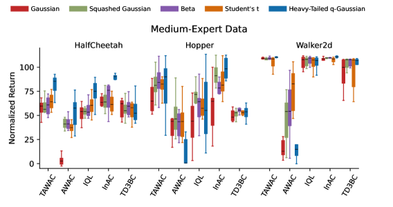
Our offline experiments comprise 3 environments, 3 datasets, 5 agents, and 5 policies. We sweep hyperparameters with 5 seeds and run extra 5 seeds for the best hyperparameter configuration. Running time in CPU hours for each agent is approximately: AWAC=8, InAC=12, IQL=8, TD3BC=7, TAWAC=8. Therefore, the total running time on is 53,175 CPU-hours. Additionally, the total running time for sweeping the hyperparameters and evaluating the best configurations is around 23,652 CPU-hours.
D.1 Online Environments
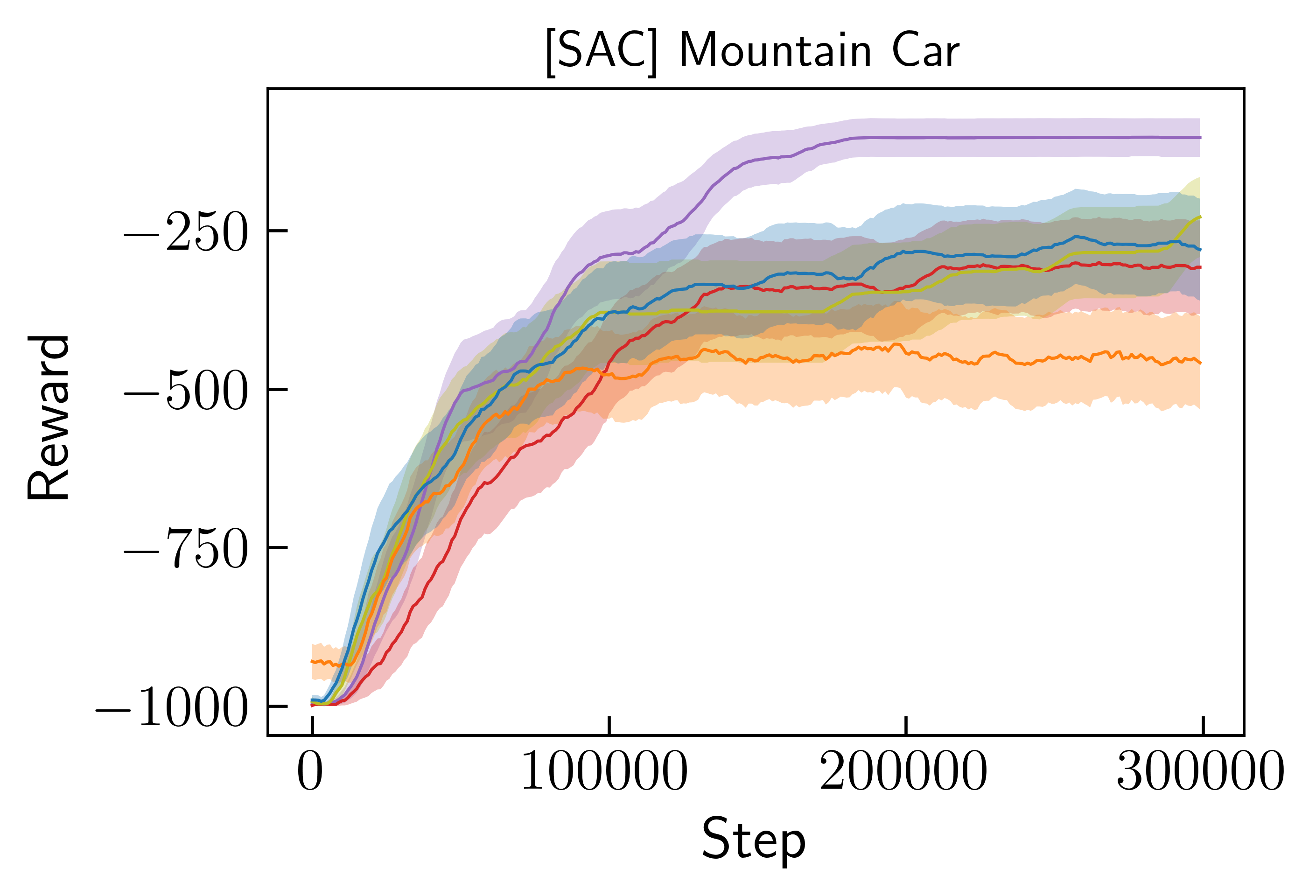
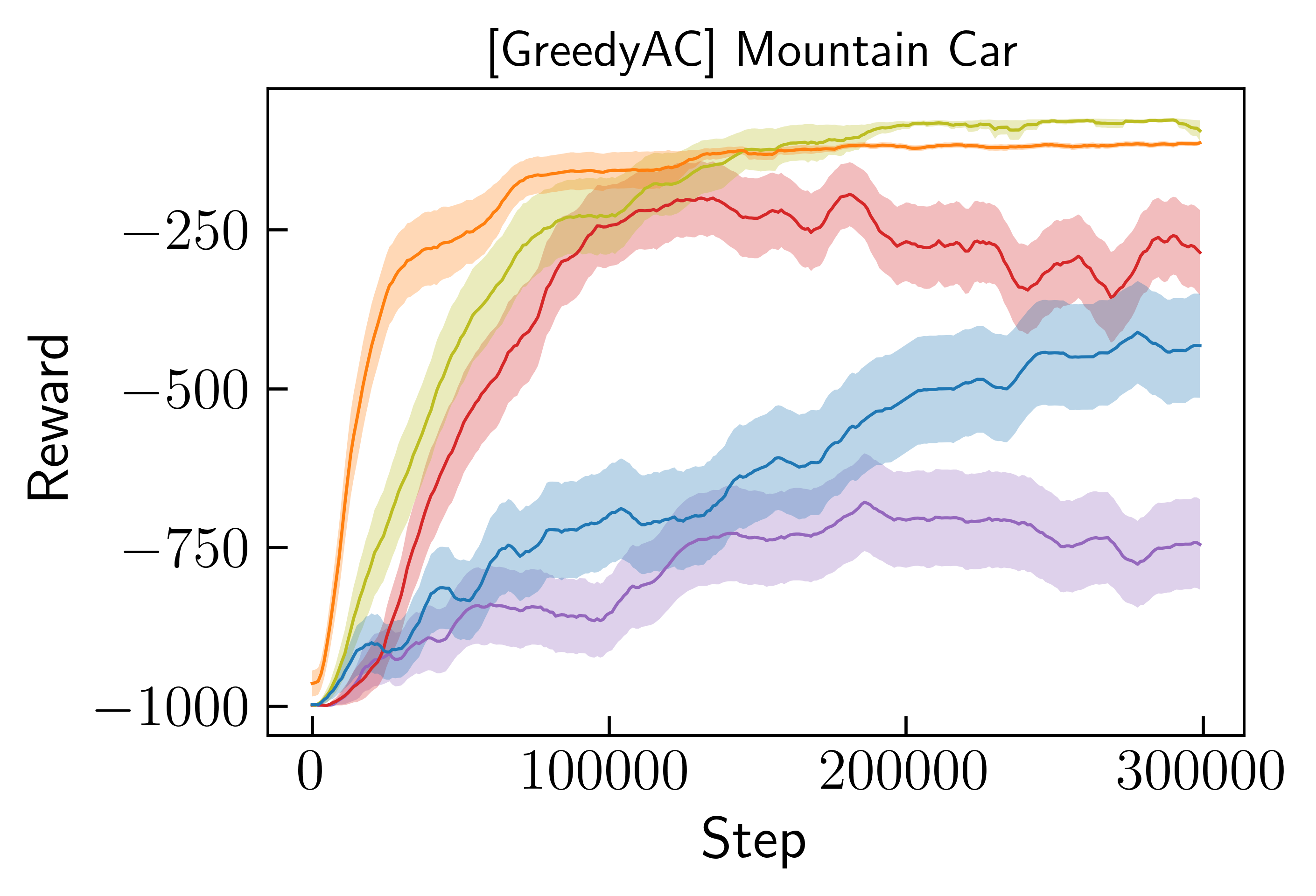
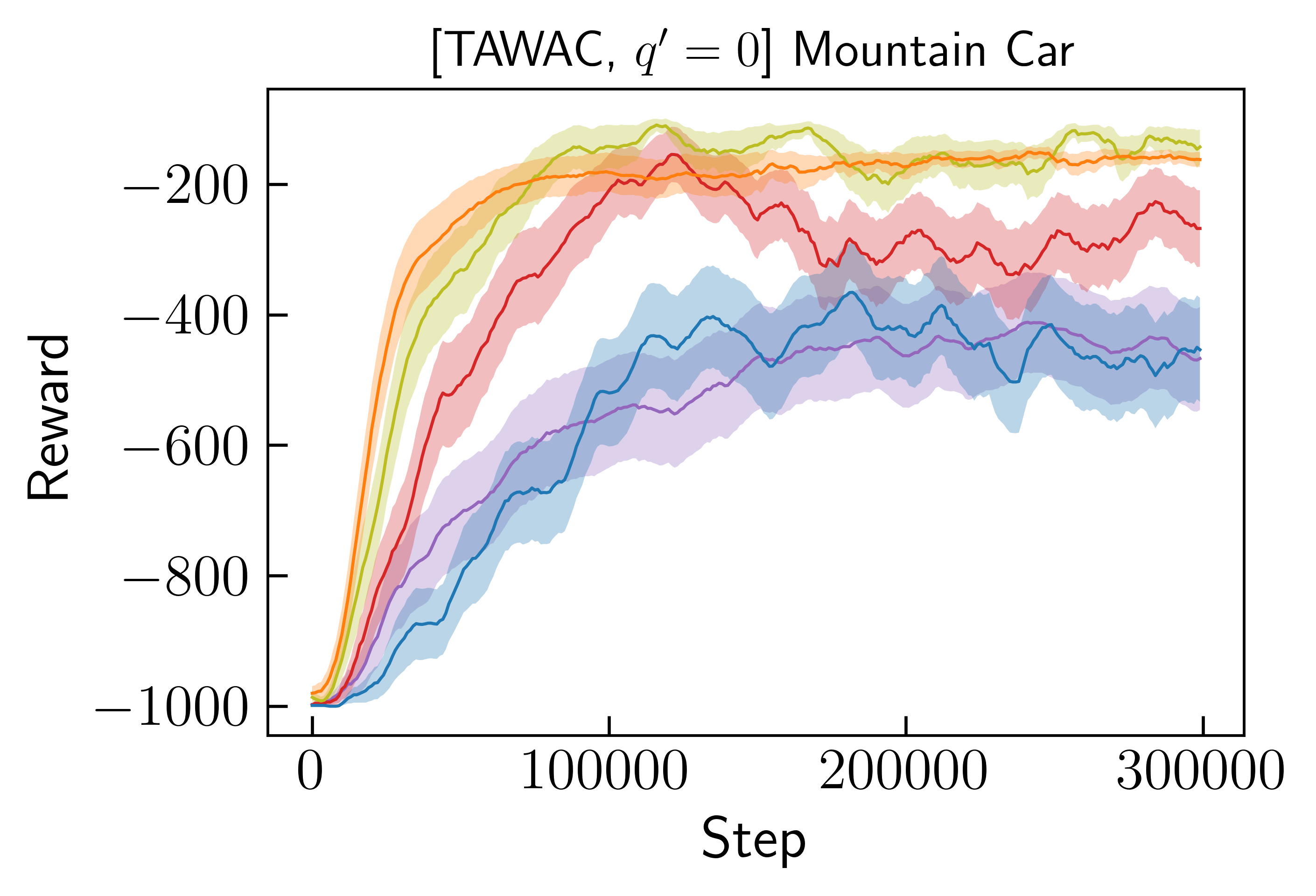
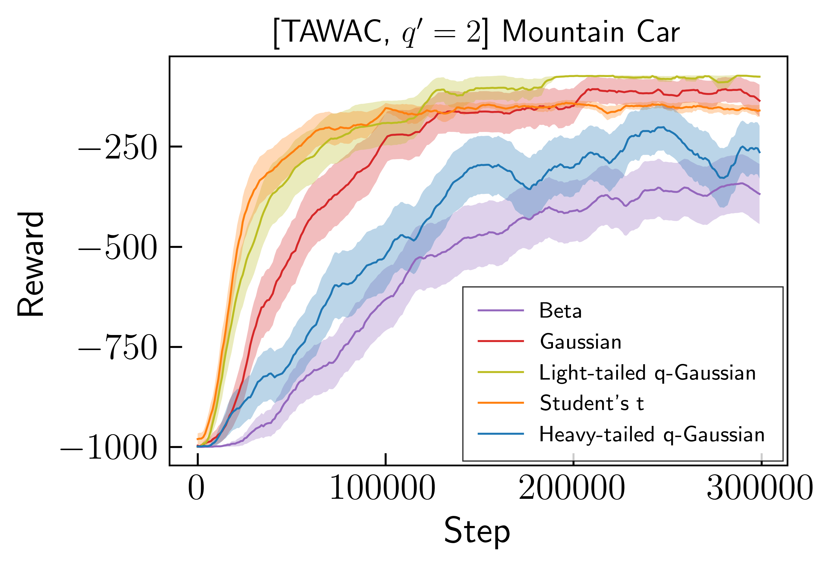
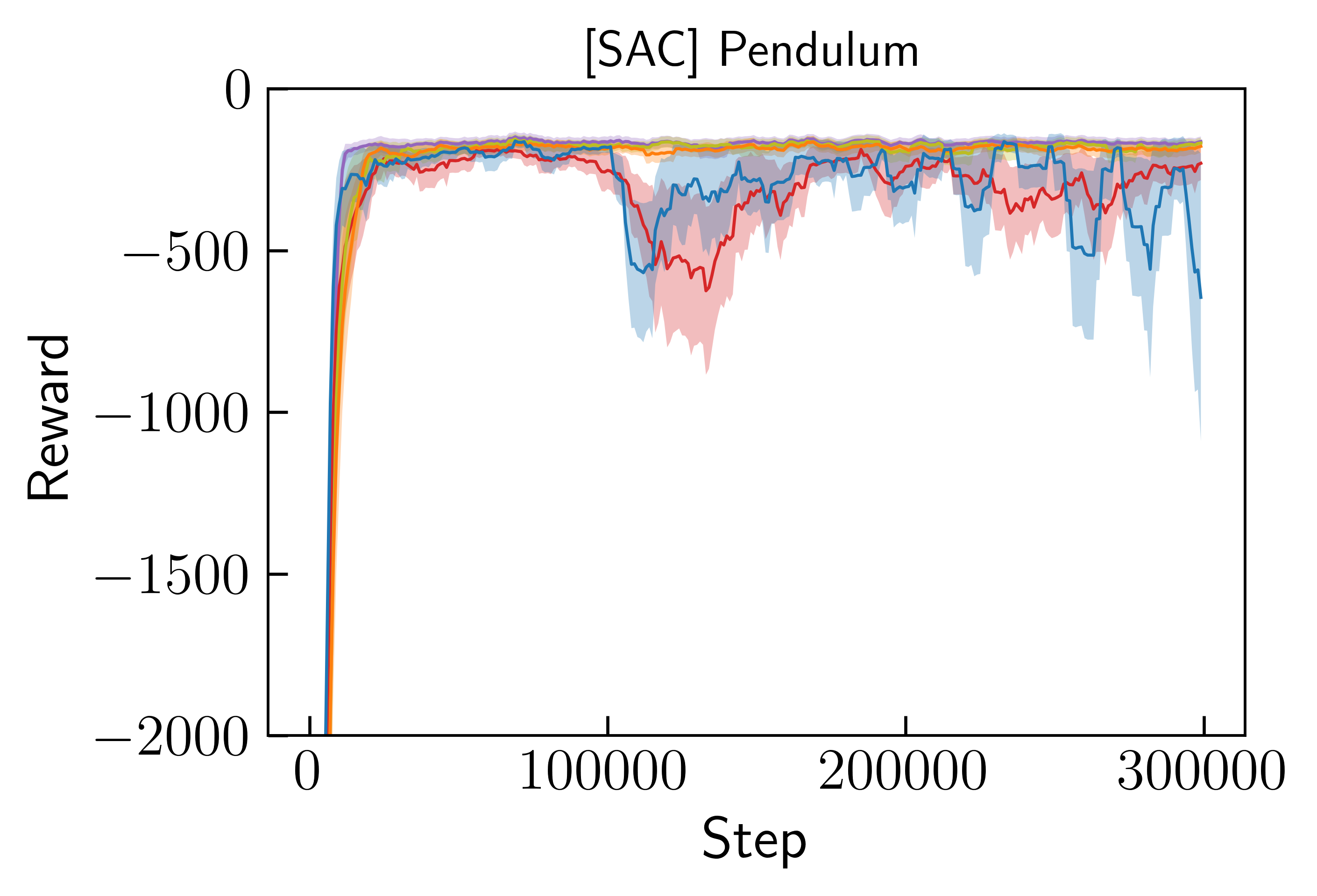
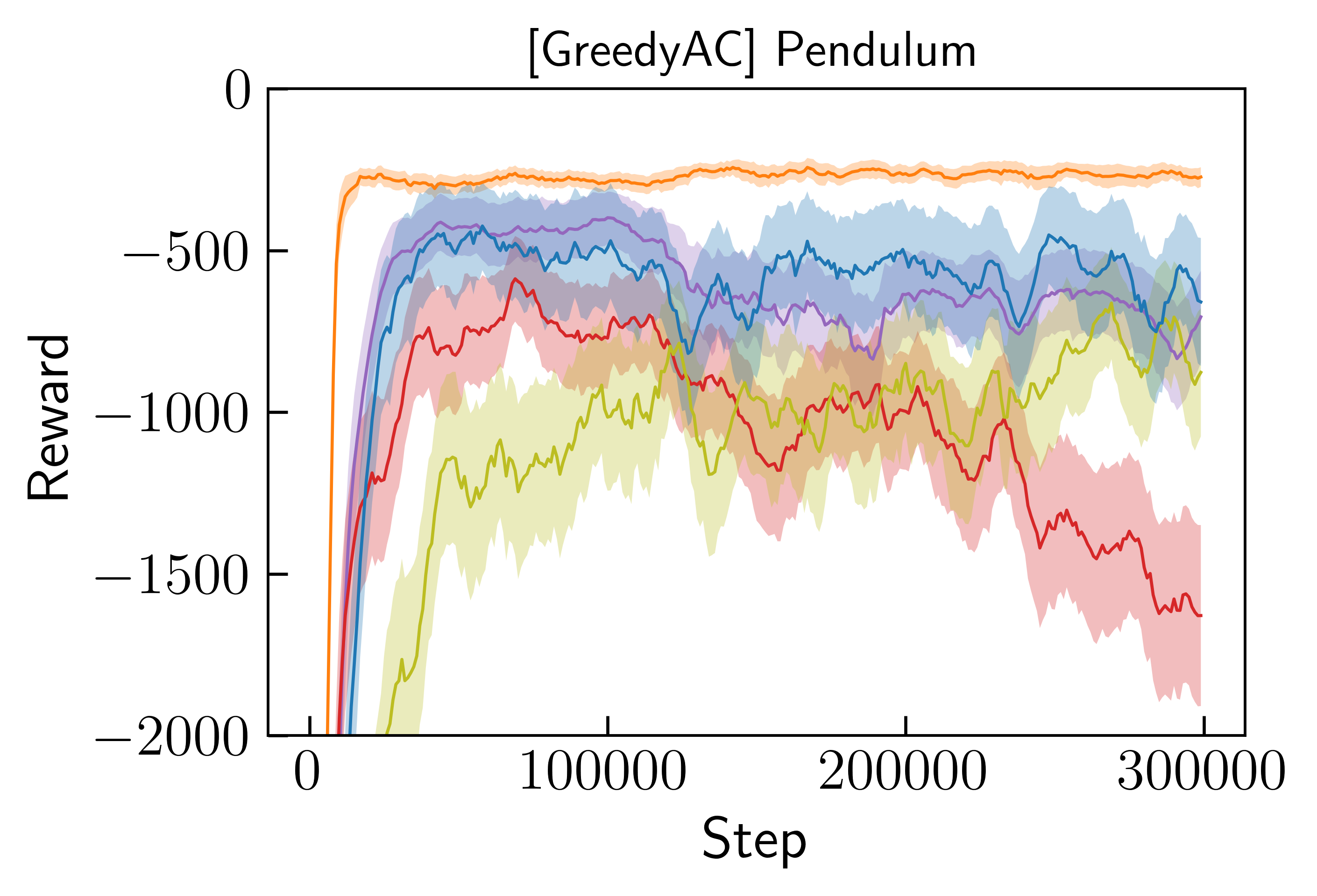
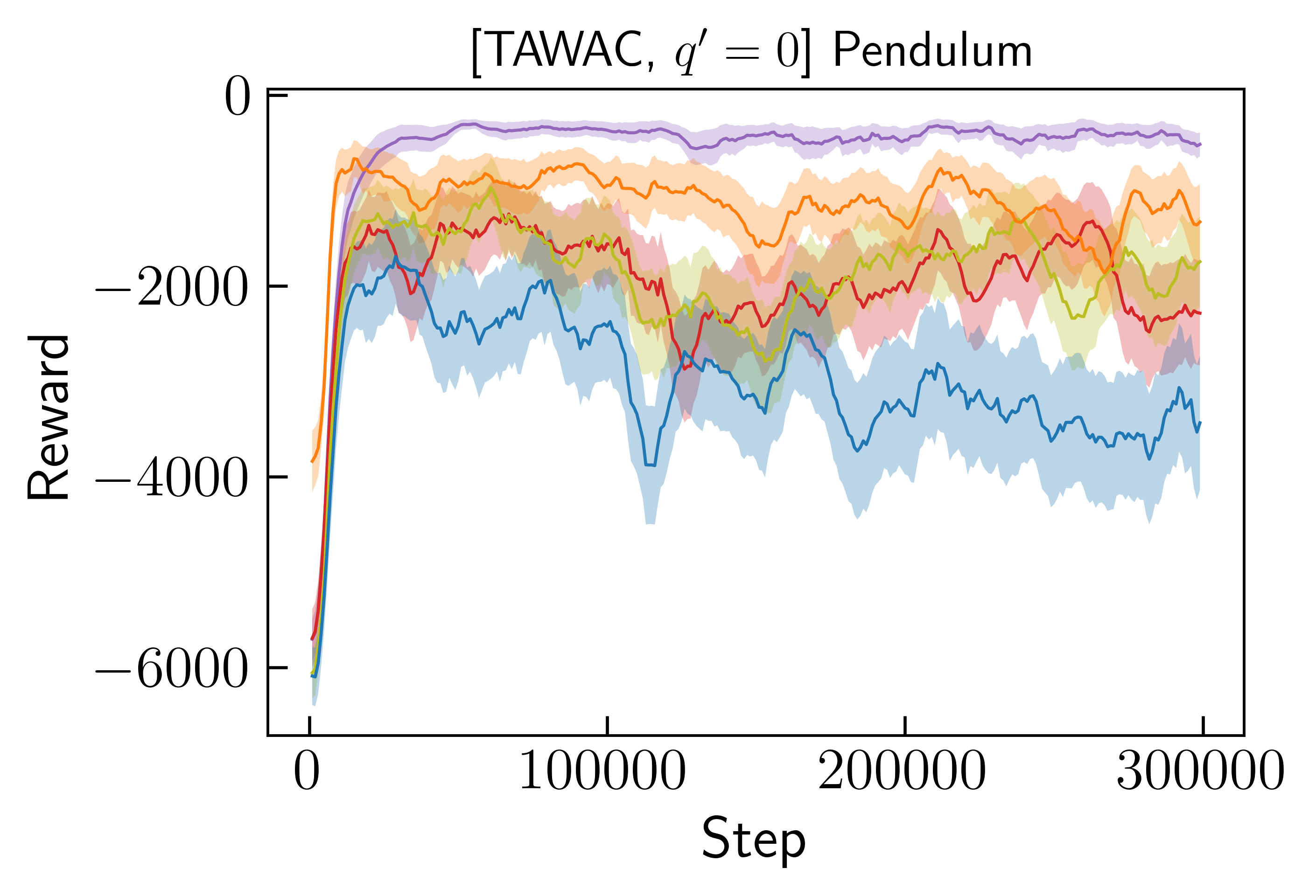
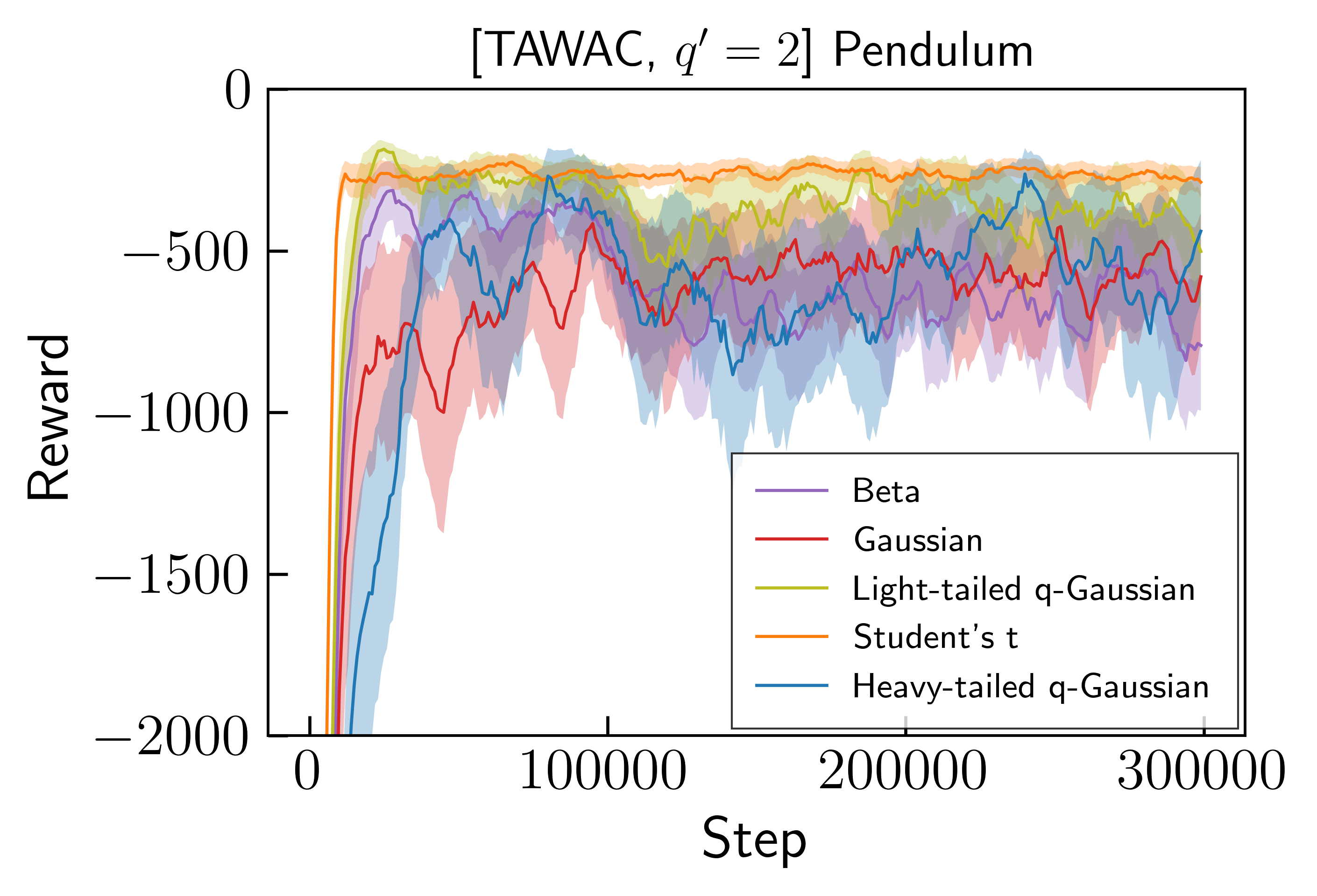
In this section we show the performance of all combinations on Mountain Car and Pendulum. Note that we have modified MountainCar to constantly reward until reaching the goal, so it requires strong exploration and encourages reaching the goal as soon as possible. For Pendulum, we only modified its maximum episode steps from 200 to 1000. When reporting the learning curve, we smoothed curves with window size 10 for better visualization.
Figure 8 shows the performance on Mountain Car. SAC + Beta outperformed other policies by a large margin. By contrast, GreedyAC and TAWAC tend to favor Student’s t and light-tailed -Gaussian. Same as in Acrobot, Gaussian tends to oscillate and converge to suboptimal scores.
Figure 9 compares the combinations on Pendulum. Surprisingly, on this environment algorithms differ the most: SAC + all policies learned equally well; while the ranking of performance drastically changes for GreedyAC and TAWAC. Despite the different rankings, Student’s t is in general performant. Another consistent observation is that Gaussian tends to exhibit large oscillations.
D.2 Offline Environments
Here we show the results of all algorithm-policy combination on all environments. We also include TD3BC [Fujimoto and Gu, 2021] for comparison.
Figure 10 shows the overall comparison with TD3. It is clear that Squashed Gaussian performs well and Beta can show slight improvements in some cases. Though it is visible that no much difference is shown except on the Medium-Replay data. We conjecture that the better performance of Squashed Gaussian and Beta could be due to the TD3BC behavior cloning loss. It is encouraged that policy closely approximates the actions from the dataset. Therefore, policies like Beta that can concentrate faster may be more advantageous.
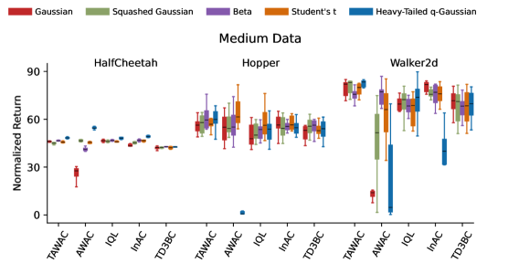
Figures 11 to 13 display boxplots of the combinations on environments of each level. Consistent observations to that in the main text can be drawn from these plots, but with the exception that in Figure 12 the environment-wise best combination is TAWAC + Student’s t. TD3BC does not exhibit strong sensitivity to the choice of policy.
Figure 14 shows policy evolution on all 6 action dimensions. It is visible that Student’s t is flexible in that on some dimensions it can take on a Gaussian shape by having large DOF and with more heavier tails on the others. Lastly, for all of the results shown above, their learning curves are shown in Figures 15 to 19. We smoothed the curves with window size 10 for better visualization.

