Estimating the FDR of variable selection
Abstract
We introduce a generic estimator for the false discovery rate of any model selection procedure, in common statistical modeling settings including the Gaussian linear model, Gaussian graphical model, and model-X setting. We prove that our method has a conservative (non-negative) bias in finite samples under standard statistical assumptions, and provide a bootstrap method for assessing its standard error. For methods like the Lasso, forward-stepwise regression, and the graphical Lasso, our estimator serves as a valuable companion to cross-validation, illuminating the tradeoff between prediction error and variable selection accuracy as a function of the model complexity parameter.
1 Introduction
When deciding which variables to include in a statistical model, a data analyst commonly wants to balance multiple goals including predictive accuracy, accurate detection of signal variables, parsimony, and interpretability. Perhaps the best-known paradigm is to use a variable-selecting method such as the Lasso (Tibshirani, 1996), forward stepwise regression (Hocking, 1976), or the graphical Lasso (Friedman et al., 2008), with a tuning parameter that controls the model complexity, and select the value of the tuning parameter by minimizing the cross-validation (CV) estimate of out-of-sample prediction error. This paradigm is versatile but prioritizes prediction error above all else, while ignoring the other goals mentioned above. In particular, CV can be quite liberal in including irrelevant explanatory variables (see e.g. Baumann, 2003), an undesirable feature in applications where accurate variable selection is a priority.
In such applications, we could abandon estimation methods like the Lasso and instead apply multiple testing methods such as knockoffs (Barber and Candès, 2016; Candès et al., 2018), or the Benjamini–Hochberg procedure or its dependence-corrected variants (Benjamini and Hochberg, 1995; Benjamini and Yekutieli, 2001; Fithian and Lei, 2022), which guarantee control of the false discovery rate (FDR) at a user-specified level. However, multiple testing methods do not yield fitted models, and the model defined by including only the selected variables can have very poor fit to the data.
In this work we introduce a new approach for assessing variable selection accuracy of estimation methods like the Lasso: an estimator for the FDR of any variable selection procedure, which can be evaluated alongside the cross-validation curve to inform the analyst about the tradeoff between variable selection accuracy and prediction accuracy over the entire regularization path. Our estimator can be applied in common statistical settings including the Gaussian linear model, the Gaussian graphical model, and the nonparametric model-X framework of Candès et al. (2018), requiring no additional statistical assumptions in these settings beyond those required for standard hypothesis tests. Its bias is non-negative in finite samples and typically small, and its standard error can be assessed using the bootstrap. In the special case of thresholding independent -values for multiple hypothesis tests, our method is almost identical to the FDR estimation method advocated by Storey (2002), but slightly less conservative.
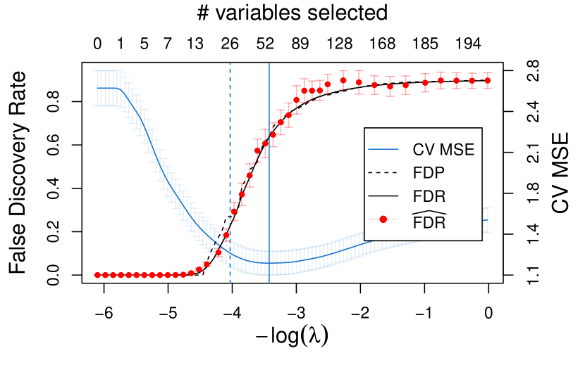
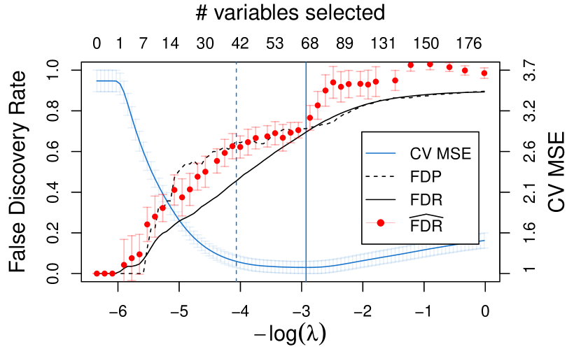
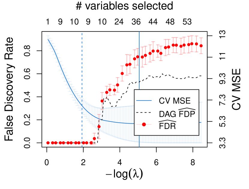
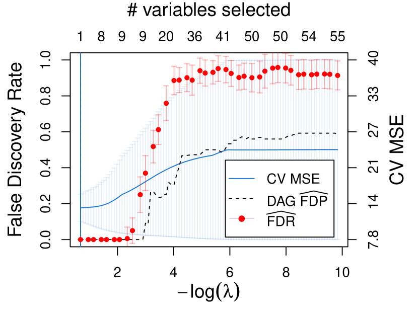
Figure 1 illustrates why our method is useful by contrasting two Lasso regression scenarios with very different tradeoffs between prediction error and FDR. In both scenarios, we generate data points from a Gaussian linear model with standard Gaussian explanatory variables, of which only are true signal variables with the same moderate signal strength. The only difference is that the explanatory variables are independent in the first scenario, but correlated in the second (specifically, they follow correlation). This difference dramatically changes the variable selection performance: When the explanatory variables are independent, it is possible to select a good predictive model if we use the one-standard-error rule (but not if we minimize CV error). When the explanatory variables are correlated, however, all models with reasonably good predictive error have FDR exceeding . While the CV curve gives no indication of the variable selection performance in either scenario, our estimator is accurate in both. The next section explains how we calculate it.
1.1 FDR estimation in the Gaussian linear model
Although our method applies in a more general setting, the special case of the Gaussian linear model with fixed design provides a concrete and familiar context in which to introduce our key ideas. In this model, we assume
| (1) |
where and denote the vectors of observed values of the explanatory variables and outcome variable , respectively, and denotes the -by- matrix of all observed explanatory variables. We call a noise variable if the hypothesis is true and a signal variable otherwise. is assumed to be fixed with , while and are assumed to be unknown.
Any variable selection procedure yields an index set , which we can regard as an estimator for the set of signal variables. For example, the Lasso estimator for a fixed regularization parameter selects where
| (2) |
By contrast, forward stepwise regression (FS) selects variables by starting from the null model and adding one variable at a time, greedily minimizing at each step the next model’s residual sum of squares. After steps, the estimator is given by estimating an ordinary least squares (OLS) regression for the selected variables.
Benjamini and Hochberg (1995) define the false discovery rate (FDR) as the expectation of the false discovery proportion (FDP), defined here as the fraction of selected variables that are actually irrelevant. If is the index set of all noise variables and is the total number of selections, we have
| (3) |
using the convention that ; i.e., when no variables are selected.
Note that we can linearly decompose the FDR as
| (4) |
Using this decomposition, a promising estimator of the FDR is
| (5) |
where is the -value for the usual two-sided -test, and is a sufficient statistic under the null model . Under , the first factor in is the uniform minimum-variance unbiased (UMVU) estimator of , obtained by Rao-Blackwellization, while the second factor attempts to zero out non-null terms.
Because and are independent under , the product is an unbiased estimator for its counterpart whenever ; otherwise . As a direct consequence, we have
| (6) |
The bias of is small if most signal variables have with high probability.
The definition of our estimator in (5) is highly general and makes no assumptions about the form of the variable selection procedure . As a result, it applies to any selection procedure including the Lasso, forward stepwise regression, LARS (Efron et al., 2004), the elastic net (Zou and Hastie, 2005), and many others.
Our method requires no further assumptions beyond the standard linear model assumptions in (1) required to justify the marginal -tests for each variable. Indeed, in the common case where the method is a function of and only (which is true of all methods referenced above), the only statistical assumption required to justify the inequality (6) is that the -statistic follows a distribution under , conditional on . This assumption may hold approximately even when the parametric assumptions of the linear model fail.
As we see next, our method generalizes far beyond the Gaussian linear model to other parametric and nonparametric contexts, provided that our modeling assumptions supply an appropriate sufficient statistic for each null hypothesis . Section 2 defines our method generically and discusses additional applications including the graphical Lasso (Friedman et al., 2008) and nonparametric model-X assumptions introduced by (Candès et al., 2018). Section 3 discusses theoretical analysis of the standard error in stylized settings, as well as our bootstrap scheme for estimating the standard error, which is used to generate the error bars in all figures, and Sections 4 and 5 illustrate our method’s behavior in real data and simulation examples, respectively. Section 6 discusses computational issues, and Section 7 concludes.
2 General formulation of our estimator
2.1 Notation and statistical assumptions
Throughout the paper, we will use upper-case letters to represent variables and lower-case letters to denote individual observations. For example, is the th observation of variable and is the th observation of variable . We use the upper-case bold-face letter to denote a vector of all observations, e.g. . We use to denote the set . For , we denote as the block of matrix including only the variables in , and we use as a shorthand for and for .
We denote by a generic random object that encodes the entire data set, whose distribution we will assume lies in some known family . If is a parametric family, we generically use to denote its parameters, and to denote the corresponding distribution. In the Gaussian linear model in Section 1.1, irrelevance of explanatory variable is represented by the null hypothesis , but other problem settings will involve other null hypotheses.
To define our estimator in a generic modeling context and prove that its bias is non-negative, the sole statistical assumption we will rely on is the availability of a sufficient statistic for the submodel corresponding to each null hypothesis . In one sense this assumption is vacuous, because itself is a sufficient statistic for any model, but we will only obtain a useful estimator if encodes less information than . While not strictly required, it is also convenient to assume that there is a standard choice of -value for each , which is valid conditional on .
Section 2.4 discusses appropriate choices of and in two additional modeling settings where our method can be applied: the nonparametric model-X setting, and the Gaussian graphical model. In both examples, as in the Gaussian linear modeling example, is a complete sufficient statistic for and there exists a natural choice of which is independent of under .
2.2 FDR estimation
We now present a generic construction of our , assuming only that a sufficient statistic is available for each . Recall the decomposition (4):
To estimate each variable’s contribution , we proceed by estimating each of the two factors in turn.
Step 1: Estimating the first factor:
Crucially, note that the factor is only relevant when . As a result, we can assume when estimating it that holds. Since is sufficient for the submodel , we can do so by Rao-Blackwellizing the integrand (Rao, 1945; Blackwell, 1947), obtaining
| (7) |
For , is unbiased by construction, and it is the UMVU estimator for the first factor of whenever is complete (Lehmann and Scheffé, 1950).
Step 2: Estimating the second factor:
We could obtain a conservative estimator by simply upper-bounding the indicator , resulting in the estimator . However this estimator’s bias, while still non-negative, could be quite large. In particular, if some of the signal variables are selected with high conditional probability given , their excess contributions may be large.
A better estimator of the indicator should reliably eliminate terms for strong signal variables without introducing bias in the terms for noise variables. For any estimator , define its normalized version:
| (8) |
or if . Note we have almost surely.
Commonly there is a standard test for , whose -value is uniform and independent of under . Then, we can take for , and
| (9) |
If the signal is strong enough for the test to reject with high probability at level , then variable ’s contribution will almost always be zero. We adopt (9) as the canonical form of , using for all simulations.
Combining (7) and (8), we obtain the estimator
| (10) |
We can write the canonical version of more concretely as
| (11) |
These two factors are independent if , as is commonly the case.
The estimator derived above, in its generic form (10), is always conservatively biased:
Theorem 2.1.
Proof.
It suffices to show for all . For , is unbiased:
For , almost surely. ∎
Remark 2.1.
While we might have initially held out hope for an unbiased estimator, attaining one is typically impossible in practice. We can see this in the Gaussian linear model (1), where the FDR of any nontrivial procedure is bounded and discontinuous in , but the distribution of the response depends on in a continuous way. As a result, no statistic can have for all .
Remark 2.2.
Extending the previous remark, we might view the smoothness of with respect to , and the corresponding conservatism of , as a robustness feature of our estimator, if we have conceptual concerns about the use of point nulls in defining the FDR. If many of the parameters are minuscule, but none are exactly zero, then the formal FDR of any procedure is exactly zero, but a more practical perspective would consider these “near-nulls” to be false discoveries whenever they are selected. Because the distribution of is continuous in , it effectively treats the near-nulls as nulls. That is, while it may be a severely biased estimator for the formal FDR (which is zero), it may be nearly unbiased for the “practical FDR” that counts near-null selections as Type I errors.
Remark 2.3.
As discussed in Section 2.1, our sole statistical assumption — availability of a sufficient statistic for the submodel defined by — is formally vacuous, because is itself a sufficient statistic. However, if we take , we have
and consequently almost surely. Theorem 2.1 still applies to this estimator, which trivially has non-negative bias for the true FDR, but the estimator is useless.
Remark 2.4.
For variable selection by thresholding independent p-values at threshold , Storey (2002) proposed a conservatively biased FDR estimator
To apply our approach, let and assume . Then we have
Thus, our is nearly identical to Storey’s estimator but slightly less conservative.
The next section elaborates on our method’s definition to help readers build intuition for how it works.
2.3 Understanding our method
To better understand our method, it is helpful to consider a simpler but closely related method that we could use to estimate a different Type I error rate, called the per-family error rate (PFER)
| PFER | |||
We can follow the same approach as in Section 2.2 to obtain the PFER estimator
| (12) |
The th term in the sum (12) is an estimate of variable ’s chance of being selected, calculated under the assumption that holds. The estimator adds up these estimated selection probabilities over all variables with unimpressive -values, then multiplies the sum by an inflation factor to account for the null terms that were eliminated by chance. If , the inflation factor is .
In problems where the number of selections is relatively large and stable, such that is roughly constant conditional on , we have
and as a result
| (13) |
For variable selection methods where is deterministic, including forward stepwise regression with a fixed number of steps, this approximation is exact.
This approximation aids our intuition by telling us that is well-approximated by a sum of estimated inclusion probabilities, divided by the number of selected variables, and inflated by . Roughly speaking, is large when some unimpressive variables stood a good chance of being selected (or actually were selected), and otherwise is small.
Remark 2.5.
The PFER is interesting in its own right as an upper bound for the family-wise error rate (FWER), defined as
As a result, the estimator in (12) can also be understood as a conservatively biased estimator for FWER. We leave exploration of this extension to future work.
2.4 Example model assumptions
In this section we give additional examples beyond the Gaussian linear model and demonstrate the choices of and the ways to compute a valid -value.
Example 2.1 (Nonparametric “model-X” setting).
Candès et al. (2018) introduced novel nonparametric modeling assumptions for multiple testing in supervised learning problems, which allow the analyst to test for conditional independence between the response and each explanatory variable, given the other variables. Assume that we observe independent realizations of the -variate random vector , where the joint distribution of explanatory variables is fully known, but nothing is assumed about the conditional distribution .444These assumptions can be relaxed to allow for to be known up to some unknown parameters; see Huang and Janson (2020).
Under these modeling assumptions, is a complete sufficient statistic for the th null hypothesis . Under , after fixing the observed we can sample from the conditional distribution of by sampling a new vector according to its known distribution given . For any test statistic , we can compare the observed value to its simulated distribution to obtain a -value that is independent of ; the corresponding test is called the conditional randomization test (CRT). In our simulations, we use the marginal covariance as our CRT test statistic and perform a two-sided test, but other choices may be preferred depending on the problem setting and the manner in which the analyst expects to depend on the signal variables.
Example 2.2 (Gaussian graphical model).
Assume we observe independent realizations of a -variate Gaussian random vector (), with mean zero and positive-definite covariance matrix . In the corresponding precision matrix , the entry is zero if and only if and are conditionally independent given the other entries. In other words, the sparsity pattern of the undirected dependence graph for is identical to the sparsity pattern of . In lieu of estimating all off-diagonal entries of , a common modeling assumption is that the dependence graph is sparse, and by extension that is sparse as well (Meinshausen and Bühlmann, 2006; Yuan and Lin, 2007; Friedman et al., 2008).
We associate to each pair the null hypothesis that is absent from the true dependence graph , or equivalently . The Gaussian graphical model is a parametric exponential family model whose natural parameters are the entries of , with corresponding sufficient statistics given by the entries of , which follows a Wishart distribution. As a result, a complete sufficient statistic for is given by observing every entry of except and , or equivalently by
This sufficient statistic is strongly reminiscent of the sufficient statistic for in the Gaussian linear model, with playing the role of the design matrix and playing the role of the response, and the standard test for is indeed identical to the -test for in that regression problem. In our simulations, we use the corresponding two-sided -test -value . See Drton and Perlman (2007) for additional details.
In this modeling context, we will study the FDR of the graphical Lasso algorithm of Friedman et al. (2008), which is obtained by maximizing the log-likelihood with a Lasso penalty on the off-diagonal entries of :
| (14) |
3 Standard error of
In this section, we discuss the standard error of our estimator . Since our general method can be adapted for many different selection algorithms in many different statistical modeling contexts, it is very difficult to provide a general analysis that covers all contexts in which our method might be applied, but we can offer theoretical results in a narrower context, as well as a practical estimation strategy that we have found to be reasonably reliable in our simulation studies. Section 3.1 develops a theoretical finite-sample bound for our estimator under stylized assumptions, leading to conditions under which the variance of is vanishing, while Section 3.2 discusses a specialized bootstrap method for standard error estimation, which we use to produce all figures in this work.
3.1 Theoretical bound for standard error
Intuitively, if is reasonably large and many different variables independently have comparable chances of being selected, our estimator’s standard error should be small. To illustrate this heuristic in a stylized setting, we develop a finite-sample bound for the standard error, , for the Lasso in the Gaussian linear model, under a block-orthogonality assumption. We make no assumptions about the variables’ dependence within each block of variables, but we assume that variables in different blocks are orthogonal to each other:
Assumption 3.1 (block-orthogonal variables).
Let be an matrix, and let represent a partition of into disjoint subsets (that is, ). We say the matrix has block orthogonal variables with respect to the partition if , for all .
Assumption 3.1 allows us to treat the Lasso on the entire matrix as a separable optimization problem on the different blocks of explanatory variables. When this assumption is in effect, we will denote the size of the largest block as . We will assume throughout this section that every explanatory variable has mean zero and unit norm: and , for all . This last assumption comes with little practical loss of generality since conventional implementations of the Lasso begin by normalizing all variables in this way.
For our results below, it will be important to be able to provide a probabilistic lower bound on the average number of selections per block:
Condition 3.1 (enough selections).
We have for some .
Because Condition 3.1 always holds for some and , it has force only after we show that it holds for specific values of and , defined in terms of other problem quantities. Proposition 3.1 gives examples of such bounds for Lasso problems.
Proposition 3.1.
In the Gaussian linear model with block-orthogonal variables (Assumption 3.1), the following statements hold for the Lasso with tuning parameter :
-
1.
Let denote the probability that a Gaussian random variable with mean and variance 1 exceeds in absolute value. Then is stochastically larger than a random variable, and for any , the Lasso procedure satisfies Condition 3.1 with
-
2.
Assume no fewer than blocks contain at least one variable with for some , where is the mean of . Then is stochastically larger than a random variable, and for any , the Lasso procedure satisfies Condition 3.1 with
A finite-sample upper bound for for Lasso with block-orthogonal variables then follows.
Theorem 3.1 (finite sample variance bound).
In the Gaussian linear model with block-orthogonal variables (Assumption 3.1), suppose we apply Lasso for variable selection at , and in the form of , only depends on , the two-sided t-test p-value for , where is a -Lipschitz continuous function upper bounded by .
If Condition 3.1 holds for given values of and , we have
where the big-O notation only hides constants that depend on , , and .
Remark 3.1.
An explicit formula of the variance bound that contains , , and is provided in Appendix D.
We briefly introduce the core idea of the proof which relies on the concentration laws. Interested readers may refer to Appendix D for the full proof. Assumption 3.1 has three key consequences:
-
1.
Conditioning on fixes for every that is not in the same block as . As a result, resampling the data conditional on would not change the selection in all other blocks. Hence, the number of selections is conditionally stable: with resampling conditional on it is .
-
2.
For any , let denotes the variables in block except . The selection of variable depends on only through . Formally, we have
Note these are block-independent.555Alert readers might have noticed that conditioning on is not the same as conditioning on : there is an additional term. The analysis of the effects of is rather technical and it is the source of the term in the variance bound.
-
3.
Likewise, the p-value depends on only through . So are block-independent.
As a result, we have
The last approximation holds when with high probability and is substantially larger than . Then
This is an average of independent random variables. Therefore, the variance is of order by the concentration laws. A formal asymptotic result is shown in Corollary 3.1.
Corollary 3.1 (Asymptotically vanishing variance).
Under the same settings as in Theorem 3.1, consider a series of problems where we hold , , and fixed but allow , , and to vary as increases. Suppose that at least blocks contain a variable with , where is the mean of .
-
1.
For , suppose , and let with . Then
-
2.
For , suppose , and let with . Then
The idea of bounding by the concentration laws applies to more general settings. The key properties it requires are that 1) the selection of one variable is merely affected by a relatively small group of variables and 2) the perturbation on one variable merely affects the selection of a relatively small group of variables. For example, with the block-orthogonal variables, such a group is the block where the variable belongs to. It allows us to decouple with an individual selection and treat it as roughly constant. Then is a sum of variables with only local dependency. The independent parts of randomness in cancel each other and yield an with a small variance. However, if perturbing a single variable greatly impacts the entire selection set, can be noisy. We describe an example where has a non-vanishing standard error as increases in Appendix B.
3.2 Standard error estimation by bootstrap
In practice, we use the bootstrap to estimate the standard error to understand the noise level of . That is, we calculate the standard error of our estimator on data drawn from a distribution , where is an estimator for the true distribution . For example, we could sample i.i.d. from the empirical distribution of data in nonparametric settings (we will refer to this as the i.i.d. bootstrap), or the distribution specified by the maximum likelihood estimator (MLE) in parametric settings.
Making a good choice of for estimating requires careful consideration. One major issue with both the standard i.i.d. bootstrap and the MLE-based parametric bootstrap is that the noise variables in would all become weak signal variables in ; as a result, might select many more variables in a typical draw from (in which the true model is dense) than it would in a typical draw from , resulting in a poor estimate of the standard error of . A similar issue could arise in any parametric bootstrap method using an estimator for that is too liberal about letting variables into the model. However, an estimator that is too aggressive in shrinking signal variables could have the opposite issue, if the signal strength in is systematically smaller than the signal strength in .
To ameliorate this issue, we try to construct in such a way that most of the null variables in remain null in , but the signal variables are estimated with little bias. Formally, let denote an estimate of the index set of noise variables. In the parametric setting , we find a sparse MLE of , denoted as , under the constraints that for all . Then we set and draw bootstrap samples to calculate . We formally describe our bootstrap scheme in the parametric setting in Algorithm 1.
In our implementation, we construct as the set of variables neglected by the best model in cross-validation. More precisely, our cross-validation scheme is built to select such that the constrained MLE model is close to the true distribution . It estimates the constrained MLE with the candidate on the training set and employs the negative log-likelihood on the validation set as the error measurement. A formal description of our cross-validation algorithm is in Appendix A.2. In Section 1, we demonstrated that the model that minimizes the cross-validation error tends to over-select variables moderately: it contains most of the signal variables and a bunch of noise variables. This is exactly what we need here – to include most of the signals while roughly keeping the signal sparsity level. We give examples of the constrained MLE problem next.
Example 3.1 (Gaussian linear model).
In the Gaussian linear model, the negative log-likelihood is proportional to the mean-squared error. Therefore, is the least square coefficients regressing on variables for .
Example 3.2 (Gaussian graphical model).
In the Gaussian graphical model, we parameterize the model using the symmetric positive definite (SPD) precision matrix . Let denote the sample covariance matrix. The log-likelihood is
The constrained MLE is obtained by maximizing under the constraint that for pairs in . While there are many algorithms that can solve this problem (e.g. Yuan and Lin, 2007), we apply a simple heuristic algorithm described in Appendix A.3 to save computation.
For the model-X setting, we can employ an analogous method by using a variant of the i.i.d. bootstrap that constrains to be true for all . Specifically, we first draw bootstrap samples of from the empirical distribution of the data. Then, we sample from the conditional distribution , which is equal to under the intersection null . We formally describe our bootstrap scheme in the model-X nonparametric setting in Algorithm 2.
If the researchers make model assumptions, the set can be constructed in the same way as in the parametric settings. If no model assumption is made and the likelihood is unavailable, researchers can choose via p-value-based approaches. For example, we can calculate the conditional randomization test p-values (Candès et al., 2018) for each variable and define as all variables whose p-values are larger than . This choice lets the majority of null variables remain null in while retaining the signal for strong signal variables.
4 Real world examples
In this section we illustrate our method on real scientific data in two different modeling settings. In Section 4.1, we analyze an HIV drug resistance data set using Lasso regression, and in Section 4.2 we analyze a protein signaling network using the graphical Lasso.
4.1 HIV drug resistance studies
We first re-analyze the Human Immunodeficiency Virus (HIV) drug resistance data set of Rhee et al. (2006), who found that regularized regression algorithms were effective at predicting which in vitro virus samples would be resistant to each of 16 antiretroviral drugs, based on which genetic mutations were present in the samples. In this problem it is of scientific interest not only to predict from the virus’s genetic signature whether it would be resistant to various drugs — the focus of the original study — but also to identify which mutations best explain drug resistance, which was the focus of the re-analysis in Barber and Candès (2016). As a result, both model fit and variable selection accuracy are highly relevant, so it may be scientifically attractive to tackle both problems with a unified analysis.
Our initial processing of the data follows that of Barber and Candès (2016), yielding a different regression data set for each of 16 drugs in three different drug classes. In the data set for a given drug, the response is a measure of sample ’s resistance to that drug, and the explanatory variables are binary indicators of whether each of several hundred mutations was present or absent in that sample.
As a measure of replicability, Barber and Candès (2016) assessed whether detected genes were also present in a list of treatment-selected mutations (TSM), which a previous study had found were enriched in patients who had been treated by drugs in each of the three classes (Rhee et al., 2005). Rhee et al. (2006) also found that excluding a priori all but the TSM list of mutations was an effective form of variable selection. Following Barber and Candès (2016), we treat the TSM list, which comes from an independent data set, as an imperfect approximation to the “ground truth” set of signal mutations.666In addition to the TSM list, we include a small number of variables with extreme -statistics as “ground truth” signals in each regression. Specifically, we consider all variables rejected by the Bonferroni procedure at level to be “ground truth” signal variables. Having an estimate of the ground truth from another data set allows us to assess our estimator’s effectiveness in measuring the true FDR in this example; in most scientific problems, the ground truth is unavailable and we would have to rely on our method to measure FDR on its own.
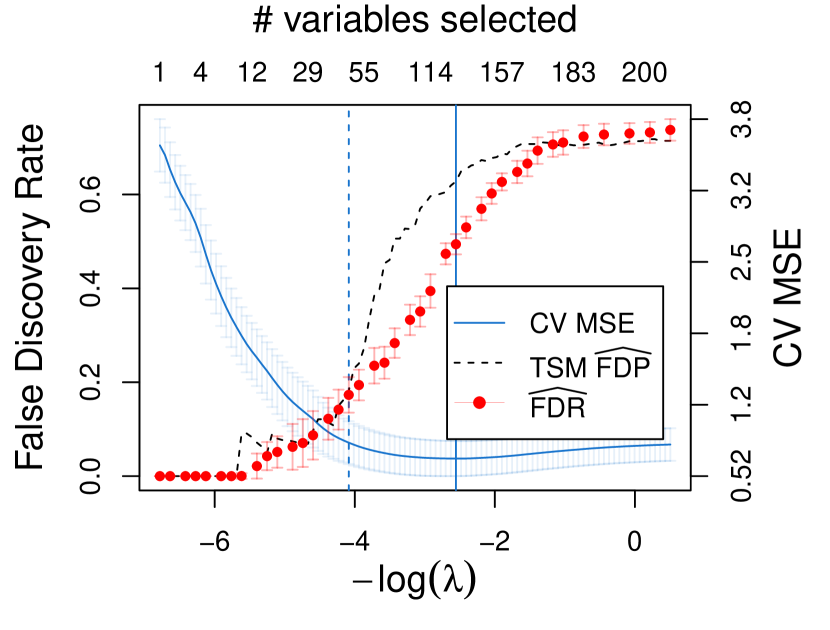
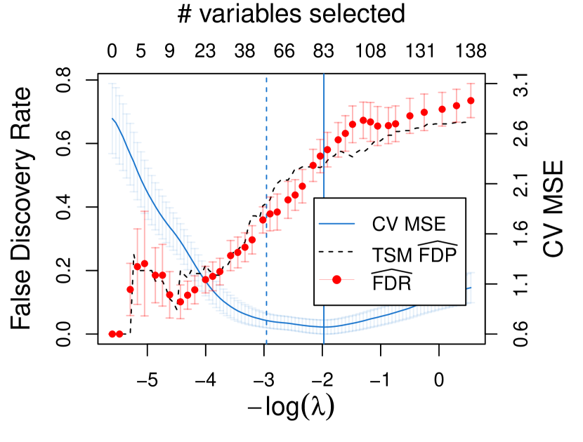


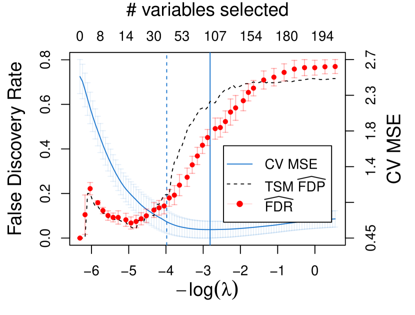
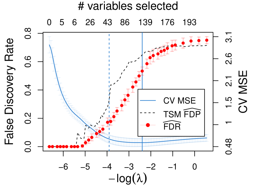
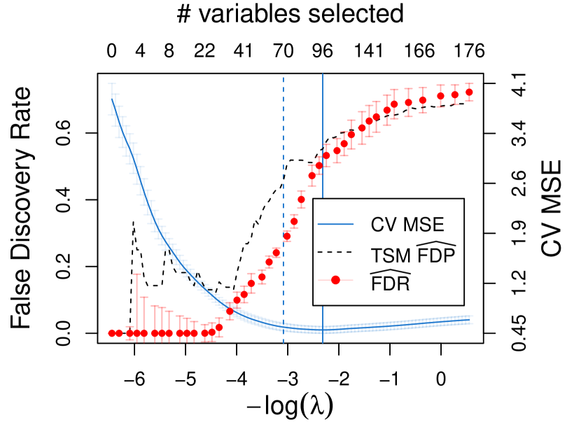
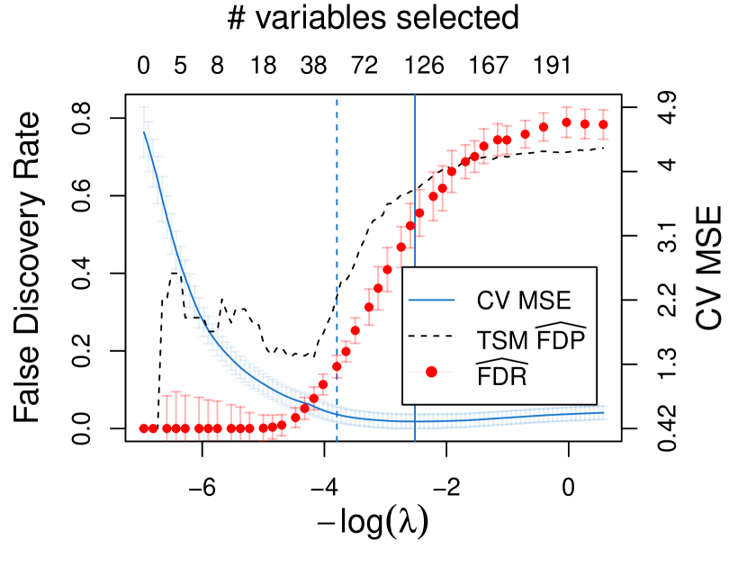
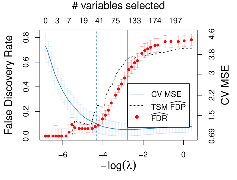
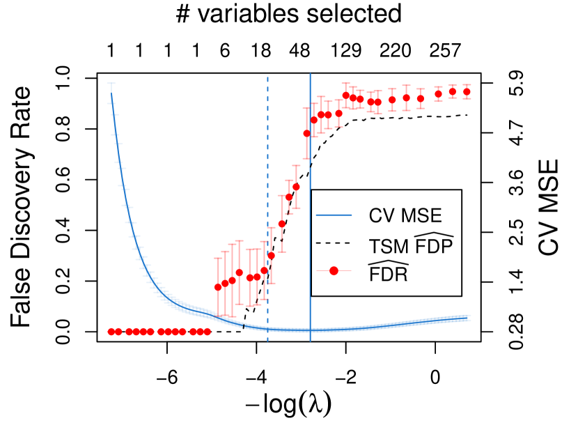
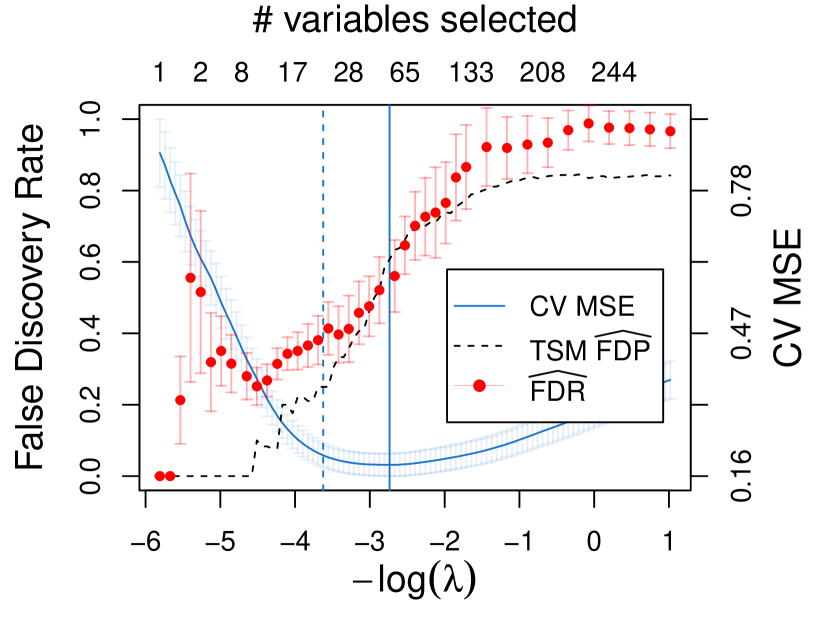
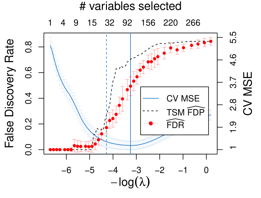
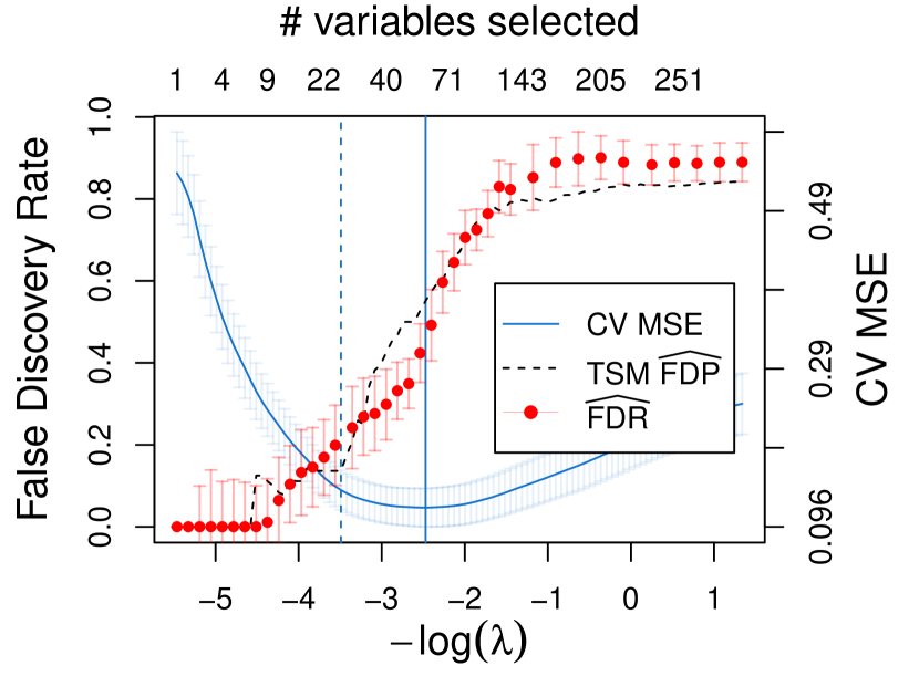
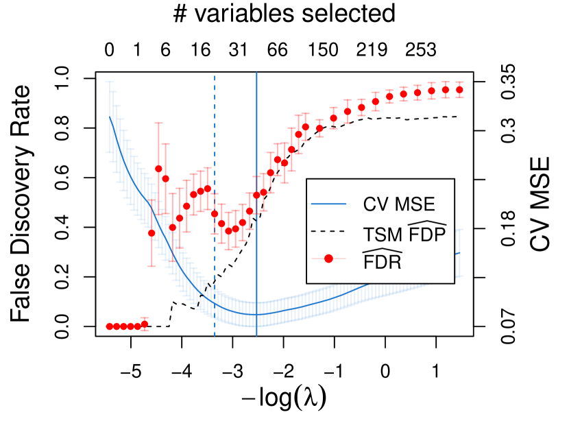
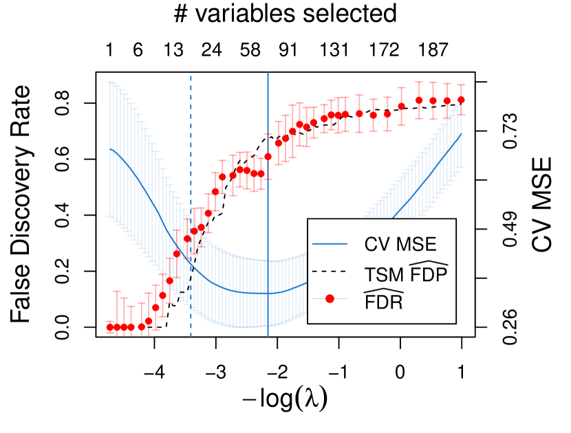
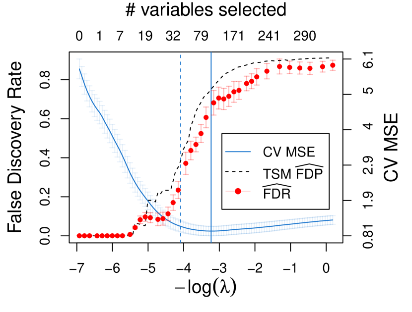
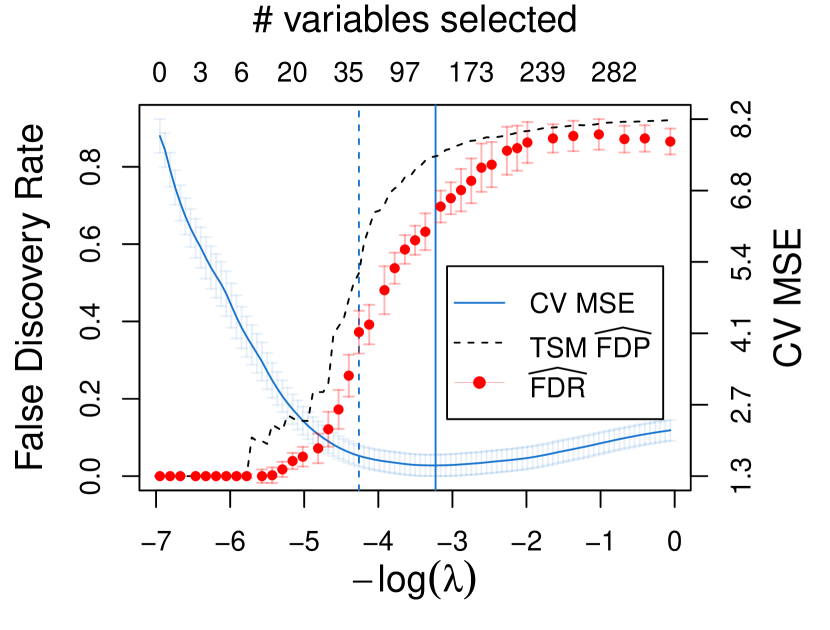
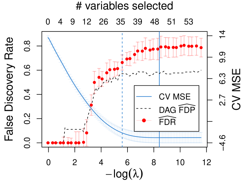
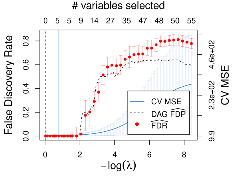
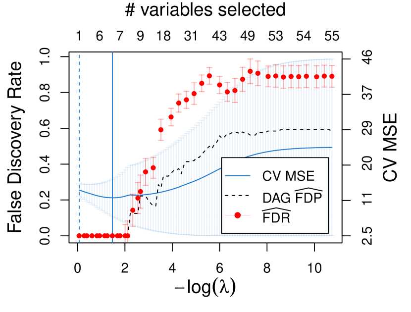
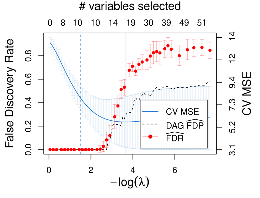
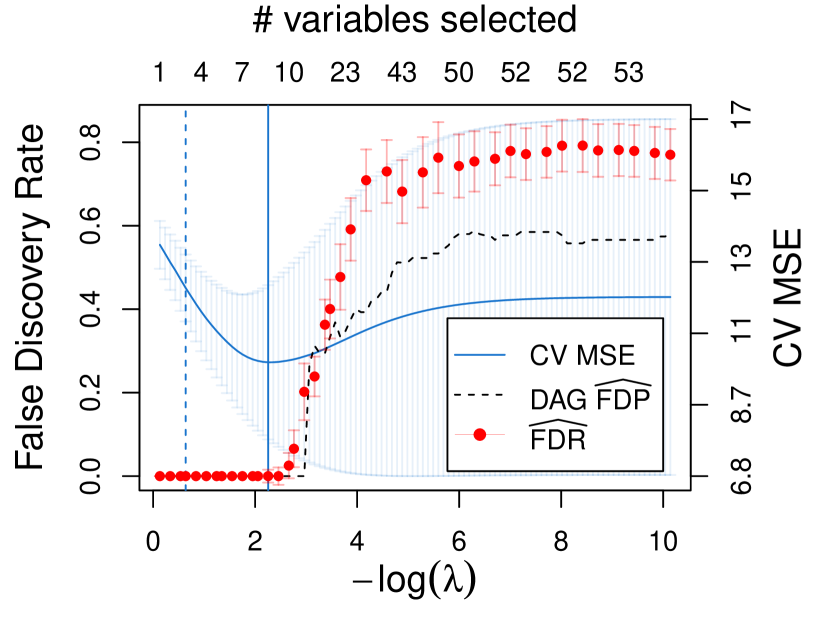
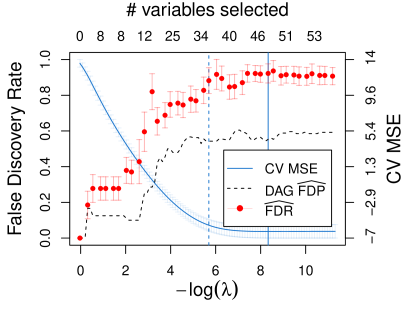
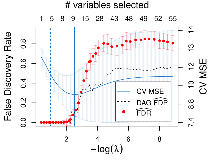
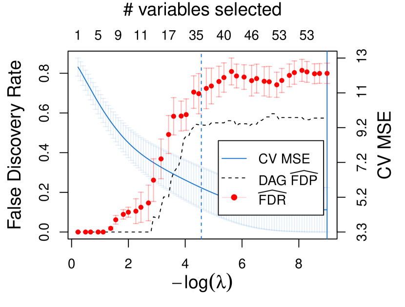
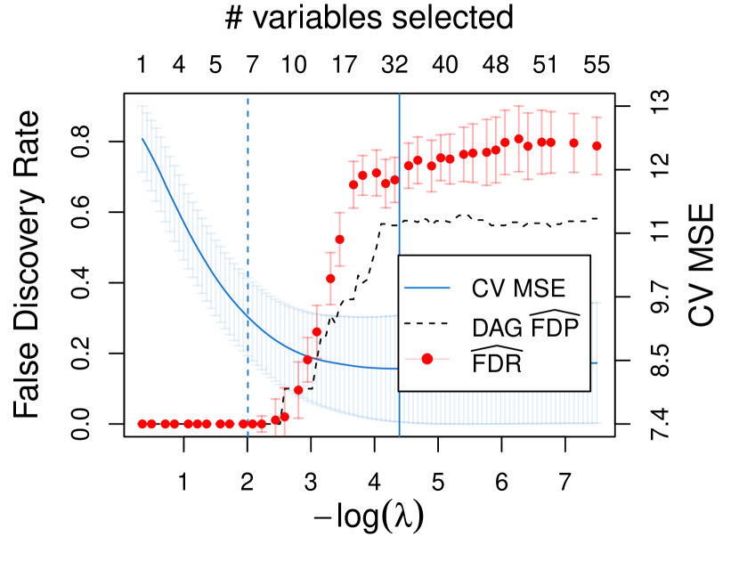
Figure 2 shows our FDR estimates alongside the CV estimate of MSE, for four selected experiments representing a variety of statistical scenarios. Results for all drugs are available in Appendix E. The error bars for both CV and our estimator show one standard error of estimated by bootstrap. The curves in the figures are estimated using the TSM signals as an approximation to the ground truth.
The four panels of Figure 2 illustrate how different variable selection problems can have very different trade-offs between variable selection accuracy and prediction accuracy. These scenarios would be impossible to distinguish from inspecting the CV curves, but our estimator is quite effective in distinguishing them from each other. Panel (a) shows an experiment in which variable selection appears to be easy: the one-standard-error rule simultaneously achieves good model fit and low FDR. Panel (b), by contrast, shows a regime in which no lasso estimator can simultaneously achieve competitive model fit and low FDR. Panel (c) shows an experiment in which the estimated FDR is non-monotone in the complexity parameter : both our estimator and the TSM judge the fifth variable to enter the model, gene P71.V, to be a likely noise variable, because its -statistic is , corresponding to a -value of , and it is also absent from the TSM list (the -statistics for the first four variables to enter all exceed 5). Panel (d) shows one of the three experiments in which our departs substantially from the TSM . In this experiment, our estimator is large mainly because three of the first five selected variables have -values equal to , , and , but the TSM curve is small because all three variables appear in the TSM list.
4.2 Protein-signaling network
To test our method in a realistic Gaussian graphical model setting, we use the flow cytometry data from Sachs et al. (2005), which Friedman et al. (2008) employed as an illustrative example in their graphical Lasso paper. The data set records levels of proteins in individual cells under different perturbation conditions, in order to estimate relationships in the protein signaling network. For each experimental condition, a sample of cells received a different biological stimulation, and the cells’ protein levels were observed.
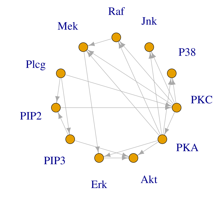
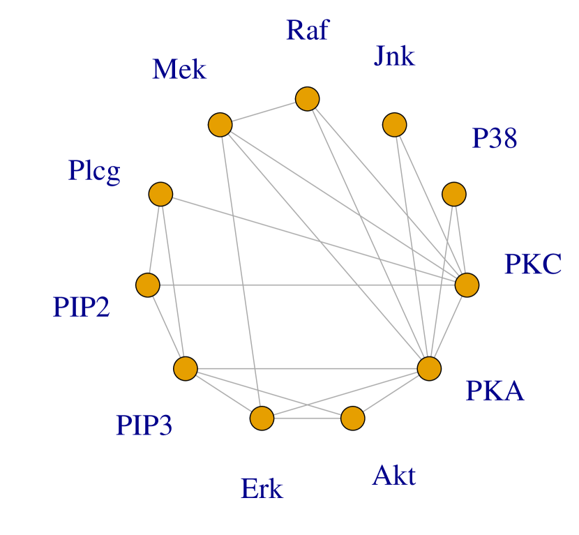
Sachs et al. (2005) supplied a causal directed acyclic graph (DAG) on the proteins, shown here in Figure 3(a). The causal graph was based on theoretical and empirical knowledge from previous literature and validation experiments that were independent from the flow cytometry dataset analyzed by Friedman et al. (2008). After converting the directed causal graph to its induced undirected conditional dependence graph, shown in Figure 3(b), we obtain an estimate of the set of true signals. As in the HIV data set, we also include as ground truth signals in each experiment a few additional pairs for which the -values pass the Bonferroni threshold at level ; i.e., those whose -statistic -values are below . Similarly to the TSM list in the HIV data set, the set of edges obtained above functions as an approximation to the ground truth, giving us a point of reference to help evaluate our FDR estimator.
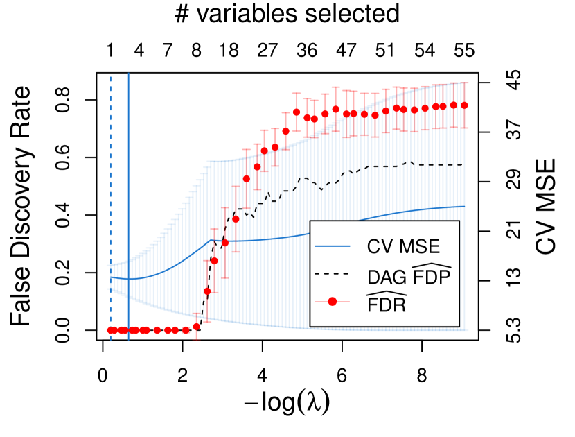

Figure 4 shows two representative examples of the results from running the graphical Lasso on the experimental settings. Results for all experiments are available in Appendix E. As in the HIV study, we show our and its estimated standard error, alongside an estimate of FDP calculated using the causal DAG supplied by Sachs et al. (2005) (denoted as the DAG in Figure 4), and the CV estimate of the predictive log-likelihood. In both panels of Figure 4, the models that we would select by cross-validation are nearly useless: one selects almost no edges, while the other selects every edge. Friedman et al. (2008) analyzed the data somewhat differently than we did, pooling all experiments together, but likewise reported that the CV curve continuously decreased until all edges were present in the model. By contrast, our gives useful information about the selection accuracy, and suggests in each experiment a natural stopping point.
The main way in which the curves in all experiments depart from the DAG estimates is that our method consistently estimates the FDR to be a bit larger across the board. The reason for this departure is that the evidence for a number of the edges identified in the DAG appears to be very weak in the data sets we analyze. That is, some of the “ground truth” edges identified by Sachs et al. (2005) appear to be absent in the actual data. This fact does not imply that those edges are truly absent in the data set, but if they are present their signals are quite weak, so our estimator treats them as likely nulls and thereby “overestimates” the FDR.
5 Simulation studies
5.1 Gaussian linear model
In this section, we evaluate the performance of in simulation environments where the ground truth is known. We begin with the Gaussian linear model and employ Lasso as the variable selection procedure.
The explanatory variables are generated under four primary scenarios, which cover independent, positively correlated, and negatively correlated explanatory variables as well as sparse matrices:
-
1.
IID normal: independent Gaussian random variables .
-
2.
Auto-regression (X-AR): ( is an AR(1) Gaussian random process with .
-
3.
Regression coefficients auto-regression (Coef-AR): The OLS coefficients ( follow an AR(1) Gaussian random process with . That is, Cov(X) is banded with negative off-diagonal entries.
-
4.
Sparse: Independent sparse binary observations .
The signal variable set is a random subset of that has cardinality , uniformly distributed among all such subsets. To mimic realistic scenarios where there is a mix between weak and strong signal variables, we generate nonzero signals with random signal strength
for all , where represents a rate- exponentially distributed random variable and is a fixed value controlling the average signal strength. We calibrate a moderate signal strength such that the selection procedure will have type II error when , where FPR stands for the False Positive Rate
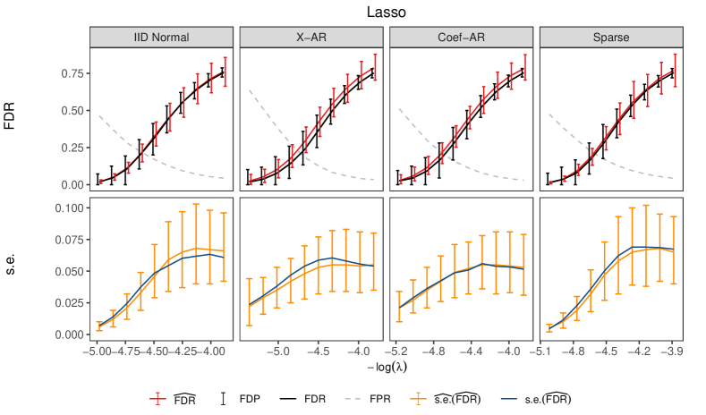
Figure 5 shows the performance of and the bootstrap with , , and . Both our estimator and our standard error estimator perform reasonably well across the board. Our shows a small non-negative bias in estimating FDR, and its uncertainty is about the same magnitude as the oracle FDP. Notably, the uncertainty of is even smaller than the uncertainty of FDP when FDR is not too large, which is the region we care most about. As for the standard error estimation, is somewhat noisy as an estimator of but roughly captures the magnitude of uncertainty of and shows relatively small bias.
Next, we stress-test the performance of in several variations on the IID normal scenario above. The other settings remain the same except for those described in each of the four scenarios below. The first three scenarios are intended to illustrate cases where may have a substantial bias and the last scenario to illustrate a case where could have a high variance.
-
1.
Weaker Signals: A weaker signal strength such that Lasso has type II error when . In this setting, only about of the signal variables have their contribution killed by the bias correction , which could potentially lead to significant bias.
-
2.
Dense Signals: We have variables and half of them are signals (). The number of observations is (same aspect ratio). This could lead to a higher bias because signal variables’ contribution is the source of bias.
-
3.
Aspect Ratio Close to 1: We have observations for variables. The IID Gaussian observations are thus closer to collinear. This could lead to higher bias because the -values we use in the bias correction are weak.
-
4.
Very Sparse: We have only signal variables, so typical model sizes are small, leading to high variance in FDP and potentially also in .
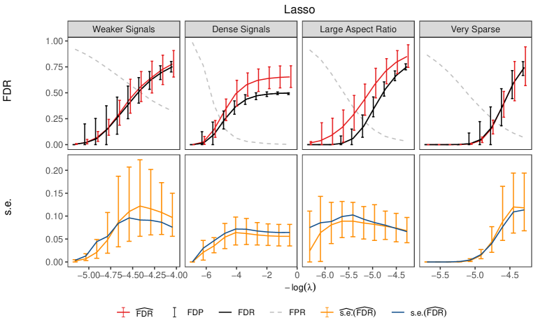
In Figure 6, does not show a substantial bias in the Weaker Signals setting, but does in the Dense Signals and Large Aspect Ratio settings when gets small. In the Weaker Signals setting, although many signal variables have , each of them contributes very little to since their probability of being selected is small under the null ; moreover, because there are many more noise variables than signal variables, the total contribution from the former is still much larger than the contribution from the latter. However, these excess contributions do cause a bias in the Dense Signals setting, because the signal variables’ total contributions is not offset by the noise variables’ total contribution. The story is a bit different in the Large Aspect Ratio setting. In this scenario, even though the signals are strong enough to be reliably detected by the Lasso, the -values are nearly powerless because the variables are nearly collinear. Hence many signal variables have . Unlike in the Weaker Signals setting, a signal variable still has a substantial chance to be selected by Lasso under due to the strong correlation structure. Therefore they make a substantial contribution to the bias. Finally, in the Very Sparse setting, we see a higher variance for owing to the typically small size of , but the FDP also has a larger variance.
5.2 Model-X setting
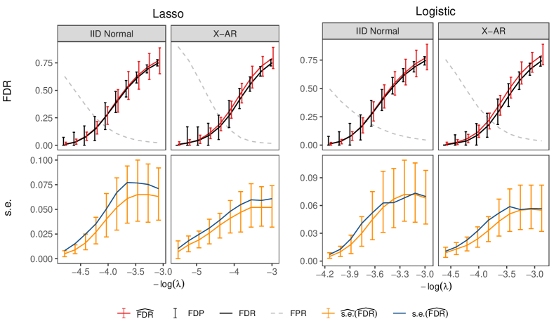
Next, we test the model-X version of our procedure in two linear modeling scenarios. The response is either a continuous response with Gaussian errors, where we employ Lasso, or a binary response that follows a logistic regression model:
where we employ -penalized logistic regression for variable selection. The other settings are the same as in Section 5.1.
5.3 Gaussian graphical model
Next, we test our method in the problem of detecting a sparse dependence graph as described in Example 2.2. We generate independent samples of variables
where and has all elements except for randomly selected upper-triangular entries. The values at these entries are again generated independently from , with calibrated such that the graphical Lasso has type II error when , and subject to the constraint that is positive semidefinite. We set , , and . Therefore, there are possible edges in the dependence graph and we apply the graphical Lasso to estimate the true edge set. Figure 8 shows the results. The bias of is very small and successfully captures the magnitude of uncertainty of .
5.4 Unfavorable case: equicorrelated Gaussian
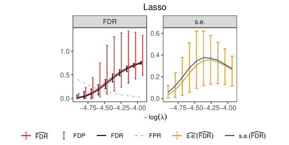
In Section 3.1, we show that has a small standard error if the variables have a block-independent structure. In this section, we examine the performance of on a practical problem with an unfavorable structure – the Multiple Comparisons to Control (MCC) problem (Dunnett, 1955), where we estimate the effects of treatments by comparing treatment group for each one to a common control group. We assume all groups have the same sample size. Mathematically, the problem is equivalent to considering -dimensional Gaussian vector , where has diagonal and off-diagonal . So all variables are positively equicorrelated: for . We are interested in selecting the signal variables with . As discussed in Section 3.1, this is an unfavorable case for .
The problem can be equivalently formalized as variable selection in a Gaussian linear model whose OLS coefficients are . We employ the Lasso selection procedure and test in this unfavorable case. Figure 9 shows the performance of and on the MCC problem with , , and signal variables. As expected, shows a nonnegative bias and an uncertainty much larger than the oracle FDP. But like in previous simulations, the tells the magnitude of uncertainty of and can warn the researchers that is not very reliable.
5.5 Robustness to model misspecification
The robustness of is closely related to the robustness of the conditional test on . Take the Gaussian linear model, for example. Figure 10 demonstrates the calculation of
on the Lasso selection procedure. Conditioning on , there is a one-to-one map between the t-statistic for and the sufficient statistic . So this conditional expectation can be calculated as a one-dimensional integral of (shown in red curve) against the -distribution density (shown in blue curve). And the calculated is the area in purple. Now consider the Gaussian linear model is misspecified. For example, the noise is not Gaussian but follows a t-distribution with degrees of freedom. The true conditional density of the t-statistic, assuming , is shown by the orange dashed curve. As expected, the conditional t-test is robust: the true density of the -statistic is not far from the theoretical -distribution density. As a result, the calculated does not change much with our misspecified model. is robust for the same reason if it is based on the t-test p-value. Therefore, we expect to be robust as long as we have confidence in the robustness of the conditional t-test on each null hypothesis.
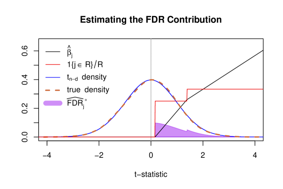
The reasoning can be extended to more general scenarios. For example, in the Gaussian graphical model with graphical Lasso selection, we expect to be robust to model misspecification if the conditional t-test on is robust. In the model-X settings, consider the selection procedures where is sufficient. These include Lasso and penalized logistic regression selection. We expect to be robust if the conditional distribution of is robust.
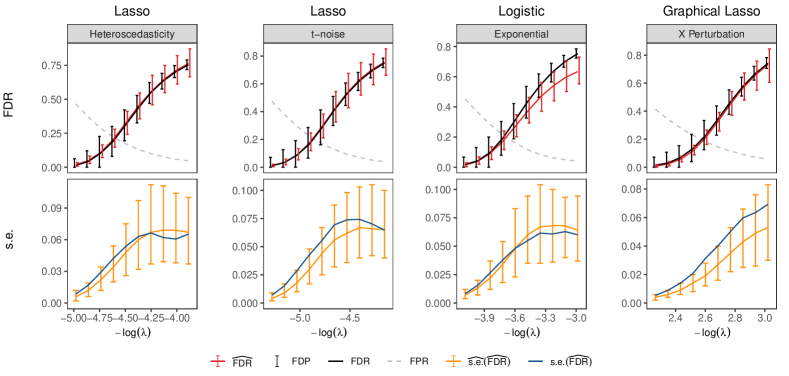
In Section 4, we have seen works well on real-world problems where the model assumptions are never exactly true. Here in Figure 11, we test the robustness of in a clean simulation study environment. We consider the same settings as previous simulations but with different types of model misspecifications. In the “Heteroscedasticity” setting, we introduce heteroscedasticity to the Gaussian linear model. That is, we generate
In the “t-noise” setting, we have the noise in the Gaussian linear model follow the t-distribution with a degree of freedom instead of the standard normal distribution. The “Exponential” setting has the variables follow the heavy-tailed exponential distribution but are mistaken as Gaussian in the model-X assumption. Finally, In the “X Perturbation” setting, we multiply each observed variable by an IID uniformly distributed perturbation . As the figure shows, our performs well in these scenarios.
6 Computational details
The major computational task in our method is to calculate conditional expectations
for with . These calculations can be easily parallelized. In a generic setting, we can use Monte-Carlo integration to approximate . The worst-case time complexity for computing is , where is the number of Monte-Carlo samples and is the running time of the selection procedure. We note that calculating the integrand of for each Monte-Carlo sample has the same computation complexity as calculating one placebo statistic in the conditional randomization test (CRT, Candès et al. (2018)) with the same selection procedure for variable . In our implementation, we use Monte-Carlo samples for computing each and Bootstrap samples.
While the Monte-Carlo procedure can work with any selection procedure, for commonly used ones like Lasso and FS under the Gaussian linear model, we can develop exact and fast algorithms by leveraging the special structures. In particular, reduces to a one-dimensional integral. We briefly describe the algorithms below and leave details in Appendix C.
Example 6.1 (fast and exact calculation of for Lasso).
Lei (2019) proposed a fast homotopy algorithm that computes the entire Lasso solution path when the sufficient statistic varies in a given direction in the context of conformal prediction. With simple modifications, we apply their algorithm to obtain the Lasso selection set for all possible values of given . This provides a full characterization of the piecewise constant function and hence yields the exact value of .
The runtime of the homotopy algorithm scales linearly in the number of knots along the homotopy path. At each knot, the algorithm applies a handful of -dimensional matrix-vector multiplications. As a result, the algorithm is faster for a reasonably large where varies less over the range of given .
Example 6.2 (fast and exact calculation of for FS).
At the -th step, the FS procedure for the Gaussian linear model selects a variable that has the largest where can be obtained by applying a sequence of normalization and orthogonalization steps. When the number of selected variables is fixed, simplifies into . The numerator can be decomposed into . We can calculate each term by using an auxiliary FS procedure that has the same computation cost as the original one. Again, each step only involves a handful of -dimensional matrix-vector multiplications. Thus, the algorithm is faster when the number of selections is small.
7 Summary
In this work we present a new approach for estimating FDR of any variable selection procedure. Our estimator can be applied in common statistical settings including the Gaussian linear model, the Gaussian graphical model, and the nonparametric model-X framework, requiring no additional statistical assumptions in these settings beyond those required for standard hypothesis tests. Our estimator can be evaluated alongside the cross-validation curve to inform the analyst about the tradeoff between variable selection accuracy and prediction accuracy over the entire regularization path. The bias of the estimator is non-negative in finite samples and typically small. The standard error can be assessed using the specialized bootstrap and it is typically vanishing when there are many variables with only local dependency. Examples with real-world and simulation data demonstrate our estimator works well in both bias and standard error. R package is available online at the Github repository https://github.com/yixiangLuo/hFDR.
Reproducibility
Our FDR estimator is implemented in an R package available online at the Github repository
github.com/yixiangLuo/hFDR.
The R code to reproduce all simulations and figures is available at github.com/yixiangLuo/hFDR_expr.
References
- Barber and Candès (2016) Rina Foygel Barber and Emmanuel J Candès. Controlling the false discovery rate via knockoffs. The Annals of Statistics, 43(5):2055–2085, 2016.
- Baumann (2003) Knut Baumann. Cross-validation as the objective function for variable-selection techniques. TrAC Trends in Analytical Chemistry, 22(6):395–406, 2003.
- Benjamini and Hochberg (1995) Yoav Benjamini and Yosef Hochberg. Controlling the false discovery rate: a practical and powerful approach to multiple testing. Journal of the Royal statistical society: series B (Methodological), 57(1):289–300, 1995.
- Benjamini and Yekutieli (2001) Yoav Benjamini and Daniel Yekutieli. The control of the false discovery rate in multiple testing under dependency. Annals of statistics, pages 1165–1188, 2001.
- Blackwell (1947) David Blackwell. Conditional expectation and unbiased sequential estimation. Annals of Mathematical Statistics, 18:105–110, 1947.
- Candès et al. (2018) Emmanuel Candès, Yingying Fan, Lucas Janson, and Jinchi Lv. Panning for gold: ‘model-X’ knockoffs for high dimensional controlled variable selection. Journal of the Royal Statistical Society: Series B (Statistical Methodology), 80(3):551–577, 2018.
- Drton and Perlman (2007) Mathias Drton and Michael D. Perlman. Multiple Testing and Error Control in Gaussian Graphical Model Selection. Statistical Science, 22(3):430 – 449, 2007.
- Dunnett (1955) Charles W Dunnett. A multiple comparison procedure for comparing several treatments with a control. Journal of the American Statistical Association, 50(272):1096–1121, 1955.
- Efron et al. (2004) Bradley Efron, Trevor Hastie, Iain Johnstone, and Robert Tibshirani. Least angle regression. The Annals of Statistics, 32(2):407 – 499, 2004.
- Fithian and Lei (2022) William Fithian and Lihua Lei. Conditional calibration for false discovery rate control under dependence. The Annals of Statistics, 50(6):3091–3118, 2022.
- Friedman et al. (2008) Jerome Friedman, Trevor Hastie, and Robert Tibshirani. Sparse inverse covariance estimation with the graphical lasso. Biostatistics, 9(3):432–441, 2008.
- Hocking (1976) Ronald R Hocking. A biometrics invited paper. the analysis and selection of variables in linear regression. Biometrics, pages 1–49, 1976.
- Huang and Janson (2020) Dongming Huang and Lucas Janson. Relaxing the assumptions of knockoffs by conditioning. The Annals of Statistics, 48(5):3021–3042, 2020.
- Lehmann and Scheffé (1950) Erich Lehmann and Henry Scheffé. Completeness, similar regions, and unbiased estimation — part i. Sankhyā: The Indian Journal of Statistics, 10(4), 1950.
- Lei (2019) Jing Lei. Fast exact conformalization of the lasso using piecewise linear homotopy. Biometrika, 106(4):749–764, 2019.
- Mathematica (2019) Mathematica. Mathematica, 2019. URL https://www.wolfram.com/mathematica.
- Meinshausen and Bühlmann (2006) Nicolai Meinshausen and Peter Bühlmann. High-dimensional graphs and variable selection with the Lasso. The Annals of Statistics, 34(3):1436 – 1462, 2006.
- Rao (1945) C.R. Rao. Information and accuracy attainable in estimation of statistical parameters. Bulletin of the Calcutta Mathematical Society, 37(3):81–91, 1945.
- Rhee et al. (2005) Soo-Yon Rhee, W Jeffrey Fessel, Andrew R Zolopa, Leo Hurley, Tommy Liu, Jonathan Taylor, Dong Phuong Nguyen, Sally Slome, Daniel Klein, Michael Horberg, et al. Hiv-1 protease and reverse-transcriptase mutations: correlations with antiretroviral therapy in subtype b isolates and implications for drug-resistance surveillance. The Journal of infectious diseases, 192(3):456–465, 2005.
- Rhee et al. (2006) Soo-Yon Rhee, Jonathan Taylor, Gauhar Wadhera, Asa Ben-Hur, Douglas L Brutlag, and Robert W Shafer. Genotypic predictors of human immunodeficiency virus type 1 drug resistance. Proceedings of the National Academy of Sciences, 103(46):17355–17360, 2006.
- Sachs et al. (2005) Karen Sachs, Omar Perez, Dana Pe’er, Douglas A Lauffenburger, and Garry P Nolan. Causal protein-signaling networks derived from multiparameter single-cell data. Science, 308(5721):523–529, 2005.
- Storey (2002) John D Storey. A direct approach to false discovery rates. Journal of the Royal Statistical Society: Series B (Statistical Methodology), 64(3):479–498, 2002.
- Tibshirani (1996) Robert Tibshirani. Regression shrinkage and selection via the lasso. Journal of the Royal Statistical Society: Series B (Methodological), 58(1):267–288, 1996.
- Yuan and Lin (2007) Ming Yuan and Yi Lin. Model selection and estimation in the gaussian graphical model. Biometrika, 94(1):19–35, 2007.
- Zou and Hastie (2005) Hui Zou and Trevor Hastie. Regularization and variable selection via the elastic net. Journal of the Royal Statistical Society Series B: Statistical Methodology, 67(2):301–320, 2005.
Appendix A Additional details in experiments and methodologies
A.1 Simulation settings for the illustrative examples
In Figure 1(a), the explanatory variables are independent Gaussian – . We have variables, observations, and variables are signal variables with random signal strength , where with are independent exponentially distributed random variable with rate . The response is generated by the Gaussian linear model with .
In Figure 1(b), the explanatory variables ( form an AR(1) Gaussian random process with . The other settings are the same as above.
A.2 Cross-validation for constructing in
In this section, we describe the cross-validation algorithm we use to construct the set in computing . Formally, let and be the th training and validation data set in a -folds cross-validation, respectively. Throughout the section, we write with as for simplicity of notation. We have
Then we find the best that achieves the largest averaged likelihood on the validation sets
and define
A.3 Sparse model estimation with graphical Lasso
We start with the unconstrained MLE
and then enforce the entries in to be zero
It is possible that the resulting is not positive definite. If that is the case, we increase the eigenvalues of by the same amount until it is positive definite.
Appendix B Example where has non-vanishing variance
We describe an example where has a non-vanishing standard error as increases.
Consider a -dimensional Gaussian vector , where has diagonal and off-diagonal . So all variables are positively equicorrelated: for . To select the signal variables with , we do a simple one-sided thresholding,
and set , where is the one-sided marginal z-test p-value. Let and . Figure 12 shows the standard deviation of does not converge to as the number of variables approach infinity.

The noisy behavior of is a consequence of the strong equicorrelation between the variables. Due to the correlation, perturbing strongly affects all other variables and hence the entire selection set. As a result, are highly positively correlated. The backbone idea for the concentration laws, which builds upon the cancellation of uncorrelated/independent noise, does not apply.
Appendix C Fast algorithms for computing
In this section, we describe the fast and exact algorithms for computing for the Lasso (Example 6.1) and FS (Example 6.2) procedures in the Gaussian linear model. Our goal is to compute
To avoid confusion, we use to refer to the particular index for which we want to compute and use to refer to a generic variable index
C.1 fast and exact calculation for Lasso
The idea is inspired by Lei (2019). Recall the Lasso coefficients are
The first-order optimal condition is
where is the dual variable satisfying for and otherwise. Suppose we have computed the selection set . Then by the optimal condition, has a explicit expression
| (15) |
Now condition on and let the value of vary. We can compute by (15) as long as does not change. The change happens when the computed becomes critical:
-
1.
an already selected variable gets kicked out of the selection set if and only if its computed coefficient become zero;
-
2.
an unselected variable gets selected if and only if the absolute value of its dual variable touches .
Readers may refer to Lei (2019) for a more detailed discussion on these two conditions.
Combine all the above. We start from a computed , let the value of vary (say increase), and calculate by (15). Once either of the two conditions is satisfied, we update and move forward. We perform a low-rank update on in (15) by the Sherman–Morrison–Woodbury formula. This algorithm reveals the exact Lasso solution path. To compute , we only care about the points of change of , which can be found by solving simple linear equations derived from the two conditions. The calculation of then becomes a one-dimensional integral of the known piecewise constant function on a known probability measure.
C.2 fast and exact calculation for FS
In the Gaussian linear model, FS first centers and normalizes the observed variables
Then do the following operations in each step.
-
1.
Selection: ;
-
2.
Gram-Schmidt orthogonalization: and for all .
-
3.
renormalization: for all .
Since we select one variable at each step, the number of selections is known. Therefore, to compute , it suffices to calculate .
Now condition on and let the value of vary. Consider an auxiliary FS procedure where we enforce that variable is not to be selected:
This auxiliary procedure is determined by the value of without looking at . At each step, if
then the variable with index , instead of , will be selected. By this inequality and certain linear transforms, we obtain the set of values of such that variable is selected at each step. Taking a union of them and using the known distribution of , we can compute . The algorithm requires one auxiliary FS process (shared among many different ) and produces a fast and exact calculation. Similar ideas apply to the model-X settings.
Appendix D Deferred proofs
In this section, we assume Assumption 3.1 and prove the propositions in Section 3.1. Throughout the section, we use to denote the selection set of Lasso. Define as the selected variables in block and as its cardinality. Throughout the section, we consider any pair of such that . We start with showing two technical lemmas.
Lemma D.1.
depends on only through . The p-value depends on only through , where .
Proof.
Let be the projection of onto the subspace spanned by the columns of , and denote the projection of onto the columns of as . Then
and the s are orthogonal to each other under Assumption 3.1. We rewrite the Lasso coefficients
We see solving for is equivalent to solving for Lasso coefficients for subproblems of regressing on . So depends on only through , which is equal to . Therefore, depends on only through .
Recall the p-value is a function of the t-statistic
The denominator depends on only through RSS. For the numerator, note is block-diagonal by the orthogonality in Assumption 3.1. We have
where is the index of variable in block . Therefore depends on only through . ∎
Lemma D.2 (mean value).
Suppose for and is integrable with respect to the measure . Then there exists some such that
Proof.
Define
Since , we have satisfies the conditions. ∎
Now we are ready to show the propositions in Section 3.1.
Proof of Proposition 3.1.
Recall in the Gaussian linear model, we conditional on the explanatory variables and treat them as fixed. By Lemma D.1 and the block-orthogonality, are independent for . Our goal is to show is stochastically larger than the sum of certain independent Bernoulli random variables. Then the proposition follows by the concentration laws.
Part 1. By Lemma D.1 and the first order condition, if and only if there exist some such that . We have
The last inequality is because that is a Gaussian random variable with variance (note is normalized). Direct calculation shows the probability achieves minimum when has mean zero.
As a consequence, is stochastically larger than , where are independent Bernoulli random variables with success probability . By the multiplicative Chernoff bound, we have
Part 2. To avoid triviality, assume is an integer. Let denote any one of the blocks that contains a variable with . Note is Gaussian with mean . By a similar reasoning as in Part 1,
As a consequence, is stochastically larger than , where are independent Bernoulli random variables with success probability . By the multiplicative Chernoff bound, we have
∎
Proof of Theorem 3.1.
Notice in (2), if we scale both and by , the optimal solution will be scaled by as well, but the selected variables do not change. Hence in the proof, we assume without loss of generality.
Let be the columns of whose indices are in and be its complement. Let be the same as but with excluded.
Under Assumption 3.1,
where and is the norm of the projection of on to the direction of . By Lemma D.1, depends on only through and depends on only through . The conditional expectation is an one-dimensional integration over . To avoid confusion, we use to denote the value corresponding to the observed and to denote a placeholder for in the integral. We write
where
and
We suppress and write for simplicity of notation. Note the measure depends on only through . Note
By Lemma D.2, for some , we have
Therefore
For notational convenience, we suppress taking maximum with for . Through out the section, we have represents and represents . Then we can write
Define
We have
and
Note we can compute from for any . Moreover, by Lemma D.1, for any , depends on only through . So depends on only through . Therefore, condition on RSS, both and are sets of conditional independent random variables respectively. We denote for simplicity.
Next we prove the theorem in three steps.
Step 1. almost surely for some that does not depend on RSS.
For simplicity of notation, we denote as and as . Let be the number in Proposition 3.1. We have
where is an IID copy of conditional on RSS. We will control each term separately. First,
The last inequality is obtained by considering cases where is positive or negative separately. Note and are conditionally independent given RSS. We have
Note , we have and . Similarly, and . Thus
and
Therefore the first term is bounded by . For the second term,
The last inequality is because . By Proposition 3.1, we have
Combine the results above, we have
The bound is of if .
Step 2. .
We start by bounding the perturbation of when we perturb RSS while holding fixed. We write
where , , and is the probability density. Direct calculation shows
Note that . By the bounded convergence theorem,
where
Note that if and only if and
Since , we have
The last equation is calculated by Mathematica (2019) and the last inequality is by and .
Then let us look at the effect of perturbing RSS on the two-sided t-test -values. We have
where is the cumulative distribution function of the t-distribution of degree of freedom . Then
Now consider the event . Recall we assume . Since is sub-exponential, we have by the Bernstein concentration equalities.
On , we have
and
Note both and are bounded. Therefore, is Lipschitz in RSS with a Lipschitz constant
Moreover, is then Lipschitz in RSS with a Lipschitz constant . A key observation is that is Lipschitz in RSS since is not a function of RSS.
Now consider the event . Since RSS is independent of , and are independent. In addition, we have .
On , we have is -Lipschitz in RSS with
Therefore, for any ,
is -Lipschitz in RSS.
For notational convenience, we denote
and
Note all , , and are bounded by .
Let be an independent copy of RSS. Then
Therefore,
Since is -Lipschitz in RSS,
where the last line uses the fact that and hence . Then we have
That is
Combining Step 1 and Step 2, we have
Finally,
The big-O notation only hides universal constant.
∎
Appendix E Extended numerical results
Figure 13 shows the extended results of along with estimated one-standard-error bars in Section 4.1 and Figure 14 shows the extended results for Section 4.2.





Appendix F Running time of in simulation problems
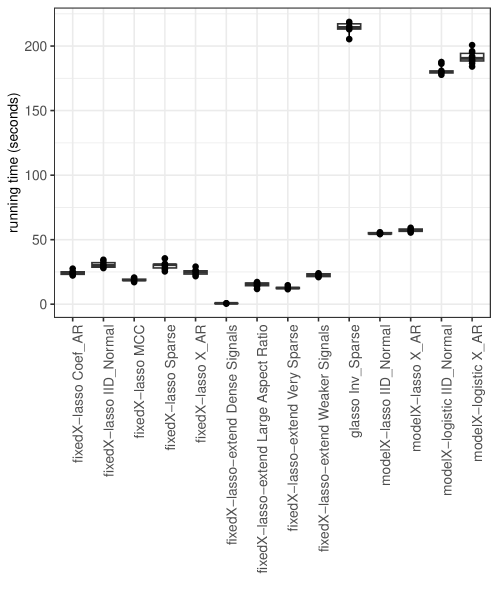
Figure 15 shows a box plot of the running time of evaluating (without estimating its s.e. by bootstrap) at all different in the the simulation problems in Section 5 on a single-cored computer. The runtime is typically several minutes.
