Causal Effect Estimation using identifiable Variational AutoEncoder with Latent Confounders and Post-Treatment Variables
Abstract
Estimating causal effects from observational data is challenging, especially in the presence of latent confounders. Much work has been done on addressing this challenge, but most of the existing research ignores the bias introduced by the post-treatment variables. In this paper, we propose a novel method of joint Variational AutoEncoder (VAE) and identifiable Variational AutoEncoder (iVAE) for learning the representations of latent confounders and latent post-treatment variables from their proxy variables, termed CPTiVAE, to achieve unbiased causal effect estimation from observational data. We further prove the identifiability in terms of the representation of latent post-treatment variables. Extensive experiments on synthetic and semi-synthetic datasets demonstrate that the CPTiVAE outperforms the state-of-the-art methods in the presence of latent confounders and post-treatment variables. We further apply CPTiVAE to a real-world dataset to show its potential application.
Deep learning models have shown great benefits in causal inference with latent variables, and increasingly, studies are utilizing the powerful representation and learning capabilities of neural networks for causal effect estimation from observational data. However, most existing studies inadvertently introduce post-treatment bias caused by post-treatment variables when making causal effect estimates from observational data. To address this, we use iVAE to learn the latent representations of post-treatment variables from their proxy variables for unbiased causal effect estimation. VAE has strong representation learning capabilities, and since post-treatment variables are affected by the treatment variable, it can effectively provide additional information during learning to ensure that the learned latent representation is identifiable. Finally, experiments on a large number of datasets show that the CPTiVAE model outperforms existing models.
Causal inference, Variational AutoEncoder, Identifiability.
1 Introduction
Causal inference promotes science by discovering, understanding, and explaining natural phenomena, and has become increasingly prominent in a variety of fields, such as economics [1, 2], social sciences [3], medicine [4], and computer science [5]. Randomized controlled trials (RCTs) are considered the gold standard for quantifying causal effects. However, conducting RCTs is often not feasible due to ethical issues, high costs, and time constraints [6]. Therefore, causal effect estimation using observational data is a common alternative to RCTs [7, 5].
In causal inference, confounders are specific variables that simultaneously affect the treatment variable and the outcome variable . For example, in medicine, a patient’s age can be a confounder when assessing the treatment effect of a drug for a particular disease. This is because younger patients are generally more likely to recover than older patients. Additionally, age can influence the choice of treatment, with different doses often prescribed to younger versus older patients for the same drug [8]. Consequently, neglecting to account for age may lead to the erroneous conclusion that the drug is highly effective in treating the disease when it is fact not.
Substantial progress has been made in developing methods to address confounding bias when estimating causal effects from observational data. Such methods include back-door adjustment [9], confounding balance [3], tree-based estimators [10] and matching methods [1]. These algorithms have achieved significant success in estimating causal effects from observational data. However, the estimation may still be biased by potential post-treatment variables affected by the treatment itself [9]. Acharya et al. [11] reported that up to 80% of observational studies were conditional on post-treatment variables.
Post-treatment variables bias the causal effect estimation from observational data. We use a simple example to illustrate this form of bias. An RCT is conducted to test whether a new drug can lower blood pressure in patients. In this scenario, the patients are randomly divided into two groups, one receiving the new drug (treatment group) and the other taking a placebo (control group). After receiving treatment, some patients become better and make lifestyle changes, such as diet and exercise. This lifestyle change may have affected their blood pressure, not just the effect of the drug itself. In this case, comparing the blood pressure levels of the two groups of patients before and after treatment may underestimate the actual effect of the new drug because post-treatment bias is not considered. Furthermore, these post-treatment variables are often unmeasured, which makes estimating causal effects more challenging. Accurate identification and adjustment of these variables are crucial for reliable causal inference.
To tackle the challenges mentioned above, we propose CPTiVAE, a novel identifiable Variational AutoEncoder (iVAE) method for unbiased causal effect estimation in the presence of latent confounders and post-treatment variables. In summary, our contributions are as follows:
-
•
We address an important and challenging problem in causal effect estimation using observational data with latent confounders and post-treatment variables.
-
•
We propose a novel algorithm that jointly utilizes Variational AutoEncoder (VAE) and Identifiable VAE (iVAE) simultaneously to learn the representations of latent confounders and post-treatment variables from proxy variables, respectively. We further prove the identifiability in terms of the representation of latent post-treatment variables. To the best of our knowledge, this is the first work to tackle both confounding and post-treatment bias in causal effect estimation.
-
•
We conduct extensive experiments on both synthetic and semi-synthetic datasets to evaluate the effectiveness of CPTiVAE. The results show that our algorithm outperforms existing methods. We also demonstrate its potential application on a real-world dataset.
2 Related Work
In recent years, numerous methods for estimating causal effects from observational data have been developed. A key challenge in performing causal inference from such data is tackling confounding bias, which becomes even more complex in the presence of latent post-treatment variables. In this section, we review some related works that address both confounding and post-treatment bias in causal inference.
Many methods assume that all confounders can be observed, i.e., the well-known unconfoundedness assumption [1]. For example, Pocock et al. [12] proposed to control for all covariates by using an adjustment strategy, and the method in Li et al. [13] balanced the covariates by re-weighting the propensity score. Some tree-based methods, such as CausalForestDML, design specific splitting criteria to estimate the causal effect [14, 15]. Furthermore, many representation learning based methods have been developed for causal effect estimation from observational data, but they generally rely on the unconfoundedness assumption. Shalit et al. [16] presented the method that shares outcome information between the treatment and control groups through representation learning while regularizing the distance of the representation distribution between the groups. Yoon et al. [17] used a Generative Adversarial Nets (GAN) framework, GANITE for estimating counterfactual outcomes based on a fitted generative adversarial network but only modelled the conditional expectation of the input outcomes. Kallus [18] used weights defined in a representation space to balance treatment groups. However, these methods do not address the bias caused by post-treatment variables.
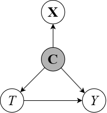
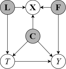
Proxy variables are commonly used for causal inference [19, 20, 21, 22, 23]. Miao et al. [20] proposed using proxies as general conditions for identifying causal effects, but this was not based on a data-driven method. Louizos et al. [19] introduced the CEVAE model (Figure 1(a)), a neural network latent model that learns the representation of proxy variables for estimating individual and population causal effects. TEDVAE (Figure 1(b)) improves upon CEVAE by disentangling the representation learning for more accurate estimation [24]. Additionally, some other Variational AutoEncoder (VAE) based estimators are related to our work. For example, -VAE [25], Factor VAE [26], HSIC-VAE [27] and -VAE [28] are both variants of VAE. However, the identifiability of the representations learned by these methods is not guaranteed.
Another line of work involves instrumental variables (IVs) methods, which are typically used to estimate causal effects when confounders are unmeasured in observational data [7]. Classical methods like the two-stage least squares model the relationship between treatments and outcomes using linear regression [29]. Advances such as kernel IV [30] and Dual IV [31] employ more complex mappings for two-stage regression. A primary challenge for IV-based methods is identifying a valid IV. These IV-based methods are not directly related to our method CPTiVAE.
In summary, traditional methods under the unconfoundedness assumption often fail to address latent confounders. Methods based on IVs can handle latent confounders, but obtaining valid instrumental variables is challenging. Methods based on representation learning and VAEs can effectively estimate causal effects from observational data but do not guarantee identifiability. Additionally, all these methods tend to overlook the presence of latent post-treatment variables, which may introduce bias in the estimation of causal effects from observational data.
3 Preliminary
Let be a Directed Acyclic Graph (DAG), where is the set of nodes and is the set of edges between the nodes. In a causal DAG, a directed edge signifies that variable of is a cause of variable of and is an effect variable of . A path from to is a directed or causal path if all edges along it are directed towards . If there is a directed path from to , is known as an ancestor of and is a descendant of . The sets of ancestors and descendants of a node are denoted as and , respectively.
Definition 1 (Markov property [9]).
Given a DAG and the joint probability distribution , satisfies the Markov property if for , is probabilistically independent of all of its non-descendants in , given the parent nodes of .
Definition 2 (Faithfulness [32]).
Given a DAG and the joint probability distribution , is faithful to a joint distribution over if and only if every independence present in is entailed by and satisfies the Markov property. A joint distribution over is faithful to if and only if is faithful to .
When the Markov property and faithfulness are satisfied, we can use -separation to infer the conditional independence between variables entailed in the DAG .
Definition 3 (-separation [9]).
A path in a DAG is said to be -separated (or blocked) by a set of nodes if and only if the path contains a chain or a fork such that the middle node is in , or the path contains an inverted fork (or collider) such that is not in and no descendant of is in .
In a DAG , a set is said to -separate from if and only if blocks every path between to . Otherwise, they are said to be -connected by , denoted as .
Definition 4 (Back-door criterion [9]).
In a DAG , for the pair of variables , a set of variables satisfy the back-door criterion in the given DAG if (1) does not contain a descendant node of ; and (2) blocks every path between and that contains an arrow to . If satisfies the back-door criterion relative to in , we have .
In this work, we define to be the set of pre-treatment variables, which are not affected by the treatment variable. We define to be the set of post-treatment variables, which are causally affected by the treatment variable. For example, when estimating the average causal effect between education and income, basic information about the individual such as age, gender, and nationality can be considered as pre-treatment variables. In this case, the individual’s abilities will improve after receiving education, such as learning some job skills through education, which can be considered as the post-treatment variable. Unfortunately, most studies have neglected post-treatment variables, treating them as pre-treatment variables, which introduces post-treatment bias into causal effect estimation.
4 The Proposed CPTiVAE Method
4.1 Problem Setting
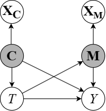
Our proposed causal model is shown in Figure 1(c). Let be the latent confounders and be the latent post-treatment variables, and are the observed proxy variables for them respectively. In this paper, confounders are variables that simultaneously affect the treatment and the outcome . Post-treatment are variables that are affected by the treatment and impact the outcome . Confounders and post-treatment variables are latent if they are not directly observed in the data. Referring to Figure 1(c), a post-treatment variable is a cause of , similar to a confounder, but the difference between them is that a confounder is a cause of treatment (i.e., ) whereas a post-treatment variable is affected by the treatment (i.e., ). For simplicity, we denote the whole proxy variables as the concatenation , where .
Let denote a binary treatment, where indicates a unit receives no treatment (control) and indicates a unit receives the treatment (treated). Let denote the observed outcomes, where and denote the potential outcomes in the control group and treatment group, respectively.
Note that, for an individual, we can only observe one of and , and those unobserved potential outcomes are called counterfactual outcomes [1, 33, 34].
The individual treatment effect (ITE) for is defined as:
| (1) |
where and are potential outcomes for individual in the treatment and control groups, respectively.
The average treatment effect (ATE) of on at the population level is defined as:
| (2) |
where indicates the expectation function.
We use the “do” operation introduced by [9], denoted as . ATE can be expressed as follows:
| (3) |
In general, ITE cannot be obtained directly from the observed data according to Eq. 1, since only one potential outcome can be observed for an individual. There are many data-driven methods for estimating ATE from observational data, but they introduce confounding bias. Covariate adjustment [35, 36] and confounding balance [16] are common methods for estimating the causal effect of on unbiasedly from observational data. To estimate the causal effect of on , the back-door criterion [9] is commonly employed to identify an adjustment set within a given DAG . Then, the set is used to adjust for confounding bias in causal effect estimations of on .
For some groups with the same features, some researchers generally use conditional average treatment effect (CATE) to approximate ITE [16], defined as:
| (4) |
In this work, we consider a problem with the presence of latent confounders and post-treatment variables . Randomization is done to establish similarity between the treatment and control groups to ensure that the treatment and control groups are similar in all but the treatment variables, which helps to eliminate latent confounders. The post-treatment variables may disrupt the balance between the treatment and control group, which eliminates the advantages of randomization [37]. Consequently, and , cannot be directly calculated using Eqs. 2 and 4. In this study, we propose the CPTiVAE algorithm to tackle the confounding bias and post-treatment bias simultaneously.
4.2 The Proposed CPTiVAE Algorithm
CPTiVAE aims to learn the latent confounder from the proxy variables , and the latent post-treatment from the proxy variables (see Figure 1(c)). Subsequently, the representations are used to address confounding and post-treatment biases.
Our CPTiVAE algorithm consists of two main components, VAE and iVAE [38]. Specifically, we use VAE to learn the representation from the proxy variables for addressing the confounding bias as done in the works [19, 24]. When the representation of confounders and the representation of the potential post-treatment variables are correct, the causal effect estimation is unbiased.
To guarantee the identifiability in terms of the learned representation by CPTiVAE, we consider the treatment as an additional observed variable and use iVAE to learn the representation from the observed proxy variables .
To guarantee the identifiability of , we take as additionally observed variables to approximate the prior [38]. Following the standard VAE [39], we use Gaussian distribution to initialize the prior distribution of and also assume the prior follows the Gaussian distribution.
In the inference model of CPTiVAE, the variational approximations of the posteriors are defined as:
| (5) | ||||
where , and , are the estimated means and variances of and , respectively.
The genereative model for and are difined as:
| (6) | ||||
where ; ; ; , and are the neural network parameterised by their own parameters. and indicate the dimensions of and , respectively. Note that and are the distributions on the -th variable.
The generative model for is defined as:
| (7) |
where is the Bernoulli function, is a neural network, is the logistic function.
Specifically, the generative models for vary depending on the types of the attribute values. For continuous , we parameterize it as a Gaussian distribution with its mean and variance given by the neural network. We define the control groups and treatment groups as and , respectively. Therefore, the generative model for is defined as:
| (8) | ||||
where , , and are the functions parameterized by neural networks, and are the means and variances of the Gaussian distributions parametrized by neural networks.
For binary , it can be similarly parameterized with a Bernoulli distribution, defined as:
| (9) |
where is a neural network.
We combine the inference model and the generative model into a single objective, and the variational evidence lower bound (ELBO) of this model is defined as:
| (10) |
where is a KL divergence term.
To ensure that is accurately predicted by , and is correctly predicted by , , and , we incorporate two auxiliary predictors into the variational ELBO. Consequently, the objective of CPTiVAE can be defined as:
| (11) |
where and are the weights for balancing the two auxiliary predictors.
4.3 Identifiability in terms of the Learned Representation by CPTiVAE
In the preceding subsections, we discussed the generative process and optimization objective of the CPTiVAE method. Now, we provide the main theorem of this paper: the identifiability in terms of the learned representation by CPTiVAE.
Let be the parameters on of the following conditional generative model:
| (12) |
where is defined as:
| (13) |
in which the value of is decomposed as , where is an independent noise variable with probability density function , i.e. is independent of or .
We assume the conditional distribution is conditional factorial with an exponential family distribution, which shows the relation between latent variables and observed variables [38].
Assumption 1.
The conditioning on is through an arbitrary function (such as a look-up table or neural network) that outputs the individual exponential family parameters . The probability density function is thus given by:
| (14) |
where is the base measure, is the normalizing constant, are the sufficient statistics, are the dependent parameters, and , the dimension of each sufficient statistic, is fixed.
To prove the identifiability of CPTiVAE, we introduce the following definitions [38]:
Definition 5 (Identifiability classes).
Let be an equivalence relation on . The Eq. 12 is identifiable up to (or -identifiable) if
| (15) |
The elements of the quotient space are called the identifiability classes.
Definition 6.
Let be the binary relation on defined as follows:
| (16) |
where is a invertible matrix and is a vector, and is the domain of .
We can conclude the identifiability of CPTiVAE as follows:
Theorem 1.
Assume that the data we observed are sampled from a generative model defined according to Eqs. 12-14, with parameters . Suppose the following conditions hold:
-
(i)
The mixture function in Eq. 13 is injective.
-
(ii)
The set has measure zero, where is the characteristic function of the density in Eq. 13.
-
(iii)
The sufficient statistics are differentiable almost everywhere, and are linearly independent on any subset of of measure greater than zero.
-
(iv)
There exist distinct points such that the matrix
(17) of size is invertible.
Then the parameters are -identifiable.
Proof.
The proof of this Theorem is based on mild assumptions. Suppose we have two sets of parameters and such that for all pairs . Then:
| (18) | ||||
| (19) | ||||
| (20) | ||||
| (21) | ||||
| (22) | ||||
| (23) | ||||
| (24) |
In Eq. 19, is the volume of a matrix . When is full column rank, , and when is invertible, . denotes the Jacobian. We made the change of variable on the left hand side, and on the right hand side.
We introduce the following equation:
| (25) |
By taking the logarithm on both side of Eq. 25 and replacing by its expression from Eq. 13, we have:
| (26) |
Let distinct points be the point provided by the assumption of the Theorem, and define . We plug each of those in Eq. 26 to obtain equations, and we subtract the first equation from the remaining equations to obtain for :
| (27) |
Let be the matrix defined in assumtion and similarly defined for ( is not necesssarily invertible). Define and the vector of all for . Then Eq. 27 can be rewritten in the matrix form:
| (28) |
Then we multiply both sides of the above equations by to find:
| (29) |
where and .
Now we show that is invertible. By definition of and according to the assumption of the Theorem, its Jacobian exists and is an matrix of rank . This implies that the Jacobian of exists and is of rank and so is . There are two cases: (1) If , is matrix of rank and invertible; (2) If , we define and . For each there exsit points such that are linearly independent. We suppose that for any choice of such points, the family is never linearly independent. That means that is included in a subspace of of the dimension at most . Let be a non-zero vector that is orthigonal to . Then for all , we have . By integrating we find that . Since this is true for all and , we conclude that the distribution is not strongly exponential, which contradicts our hypothesis.
Then, we prove is invertible. Collect points into vectors , and concatenate the Jacobian evaluated at each of those vectors horizontally into matrix and similarly define as the concatenation of the Jacobian of evaluated at those points. Then the matrix is invertible. By differentiating Eq. 29 for each , we have:
| (30) |
The invertibility of implies the invertibility of and , which completes the proof. ∎
5 Experiments
In this section, we first conduct experiments on synthetic and semi-synthetic datasets to validate that the proposed CPTiVAE can efficiently estimate causal effects with the latent confounders and post-treatment variables. We use the causal DAG in Figure 1(c) to generate synthetic datasets for evaluating the performance of CPTiVAE. We also perform a sensitivity analysis on the model parameters and verify the feasibility of the algorithm when the learned representation dimensions are different from the true covariate dimensions. Finally, we apply our CPTiVAE algorithm on a real-world dataset to demonstrate its potential application. The code is available in the appendix.
| Method | ATE | CATE | ||||||||||
|---|---|---|---|---|---|---|---|---|---|---|---|---|
| 2K | 4K | 6K | 8K | 10K | 2K | 4K | 6K | 8K | 10K | |||
| LDML | 3.01 ± 0.01 | 3.00 ± 0.01 | 3.00 ± 0.01 | 2.99 ± 0.01 | 3.00 ± 0.01 | 3.00 ± 0.01 | 3.01 ± 0.01 | 3.00 ± 0.01 | 3.00 ± 0.01 | 3.00 ± 0.01 | ||
| LDRL | 3.00 ± 0.01 | 3.01 ± 0.01 | 2.99 ± 0.01 | 3.01 ± 0.01 | 3.00 ± 0.01 | 2.99 ± 0.01 | 3.00 ± 0.01 | 3.00 ± 0.01 | 2.99 ± 0.00 | 3.00 ± 0.01 | ||
| KDML | 2.97 ± 0.01 | 2.98 ± 0.01 | 2.96 ± 0.01 | 2.97 ± 0.01 | 2.98 ± 0.01 | 2.98 ± 0.01 | 2.98 ± 0.01 | 2.97 ± 0.01 | 2.98 ± 0.01 | 2.99 ± 0.01 | ||
| CFDML | 3.00 ± 0.01 | 3.02 ± 0.01 | 3.01 ± 0.01 | 3.02 ± 0.01 | 3.01 ± 0.01 | 3.01 ± 0.01 | 3.01 ± 0.01 | 3.02 ± 0.01 | 3.00 ± 0.01 | 2.99 ± 0.01 | ||
| SLDML | 2.98 ± 0.01 | 2.99 ± 0.01 | 2.98 ± 0.01 | 2.97 ± 0.01 | 2.99 ± 0.01 | 3.00 ± 0.01 | 2.99 ± 0.01 | 3.00 ± 0.01 | 2.99 ± 0.01 | 2.98 ± 0.01 | ||
| GANITE | 2.45 ± 0.13 | 2.44 ± 0.01 | 2.46 ± 0.01 | 2.46 ± 0.01 | 2.45 ± 0.01 | 3.66 ± 0.01 | 3.67 ± 0.01 | 3.67 ± 0.01 | 3.68 ± 0.01 | 3.67 ± 0.01 | ||
| X-learner | 3.01 ± 0.01 | 3.00 ± 0.01 | 2.99 ± 0.01 | 3.00 ± 0.01 | 3.00 ± 0.01 | 3.00 ± 0.01 | 3.01 ± 0.01 | 2.99 ± 0.01 | 3.01 ± 0.01 | 3.00 ± 0.01 | ||
| R-learner | 3.02 ± 0.01 | 3.00 ± 0.01 | 3.01 ± 0.01 | 2.99 ± 0.01 | 3.00 ± 0.01 | 3.07 ± 0.01 | 3.02 ± 0.01 | 3.01 ± 0.01 | 3.01 ± 0.01 | 3.01 ± 0.01 | ||
| CEVAE | 2.93 ± 0.26 | 2.98 ± 0.37 | 1.15 ± 0.79 | 1.89 ± 0.47 | 1.59 ± 0.64 | 2.60 ± 0.65 | 2.95 ± 0.91 | 3.20 ± 0.95 | 3.54 ± 0.30 | 3.33 ± 0.66 | ||
| TEDVAE | 3.69 ± 0.02 | 3.59 ± 0.29 | 2.92 ± 0.84 | 2.87 ± 1.31 | 2.61 ± 0.76 | 3.69 ± 0.02 | 3.62 ± 0.24 | 3.21 ± 0.36 | 3.11 ± 0.67 | 2.78 ± 0.47 | ||
| CPTiVAE | 0.90 ± 0.05 | 0.84 ± 0.08 | 0.83 ± 0.03 | 0.81 ± 0.03 | 0.70 ± 0.09 | 0.92 ± 0.04 | 0.87 ± 0.05 | 0.84 ± 0.03 | 0.87 ± 0.06 | 0.82 ± 0.04 | ||
5.1 Experiment Setup
Baseline methods
We compare CPTiVAE with ten state-of-the-art causal effect estimators that are widely used to estimate ATE and CATE from observational data. LinearDML (LDML) [41], LinearDRLearner (LDRL) [42], KernelDML (KDML) [43], CausalForestDML (CFDML) [10], SparseLinearDML (SLDML) [44], GANITE [17], and Mete-learners (including X-learner and R-learner) [45] are the machine learning based estimators. There are two VAE-based estimators, CEVAE [19] and TEDVAE [24].
Evalution metrics
We report the Absolute Error (AE) to evaluate ATE estimation, where , ATE is the true causal effect and is the estimated causal effect.
We use the Precision of the Estimation of Heterogeneous Effect (PEHE) to evaluate CATE estimation, defined as,
| (31) |
where is the estimated individual treatment effect and ITE is the true individual treatment effect.
Implementation details
The implementations of LDML, LDRL, KDML, CFDML, and SLDML are from the Python package econml. The implementation of GANITE is from the authors’ GitHub111https://github.com/vanderschaarlab/mlforhealthlabpub/tree/main/alg/ganite. The implementations of X-learner and R-learner are from the Python package CausalML [48]. We use Python library pyro to achieve CEVAE and the implementation of TEDVAE is from the authors’ GitHub222https://github.com/WeijiaZhang/TEDVAE.
| Weight | Sample Sizes | ||
|---|---|---|---|
| 6K | 8K | 10K | |
| 0.89 ± 0.10 | 0.82 ± 0.40 | 0.92 ± 0.06 | |
| 0.99 ± 0.08 | 0.91 ± 0.07 | 0.99 ± 0.22 | |
| 0.83 ± 0.03 | 0.81 ± 0.13 | 0.70 ± 0.09 | |
| 1.16 ± 0.10 | 0.84 ± 0.10 | 1.09 ± 0.05 | |
| 1.08 ± 0.04 | 0.92 ± 0.03 | 1.01 ± 0.02 | |
5.2 Evalution on Synthetic Datasets
We use the causal DAG in Figure 1(c) to generate the synthetic datasets with sample sizes, 2K, 4K, 6K, 8K, and 10K for our experiments.
In the causal DAG , and are latent variables, and are the proxy variables. is generated from Bernoulli distribution. For a post-treatment variable , it is generated from the treatment variable by using , where is coefficient, is the noise term. and are generated from the latent confounder and the post-treatment variable , defined as and , where and are two coefficients. We use the Bernoulli distribution with the conditional probability to generate the treatment , defined as . Then, we can define , where is an error term.
We can obtain the true ITE for an individual based on the data generation process, and the true ATE and CATE are 1. We repeated the experiment 30 times independently for each setting to evaluate the performance of CPTiVAE.
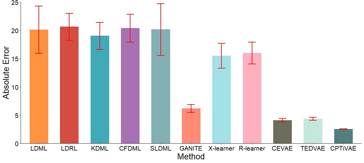
We report the AE and PEHE for synthetic datasets in Tables 1. From the experimental results, we can know that the estimators based on machine learning, i.e., LDML, LDRL, KDML, CFDML, SLDML, GANITE, X-learner and R-learner have a large AE and PEHE on synthetic datasets since these estimators cannot learn the representation from proxy variables. TEDVAE and CEVAE have a large AE and PEHE on synthetic datasets since both methods cannot tackle the latent post-treatment variables. Our CPTiVAE algorithm obtains the smallest AE and PEHE among all methods on both synthetic datasets since our CPTiVAE algorithm can learn the representation of the latent post-treatment variable from proxy variables.
In summary, the simulation experiments show that the CPTiVAE algorithm proposed in this paper can effectively address the bias introduced by the latent post-treatment variables when estimating ATE and CATE from observational data. Moreover, it further shows that CPTiVAE can recover latent variable representations from proxy variables.
5.3 Parameter Analysis
To balance and the two classifiers during the training process, we add two tuning parameters and to our CPTiVAE algorithm. We use the synthetic datasets with a sample size of 6K, 8K, and 10K, generated by the same data generation process described in Section 5.2, to analyze the sensitivity of the two parameters.
5.4 Dimensionality Study
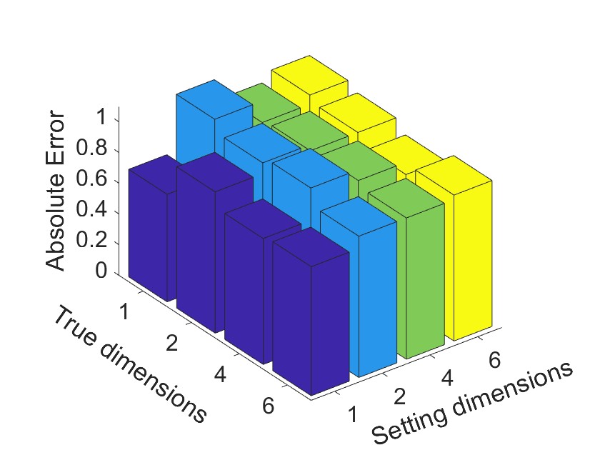
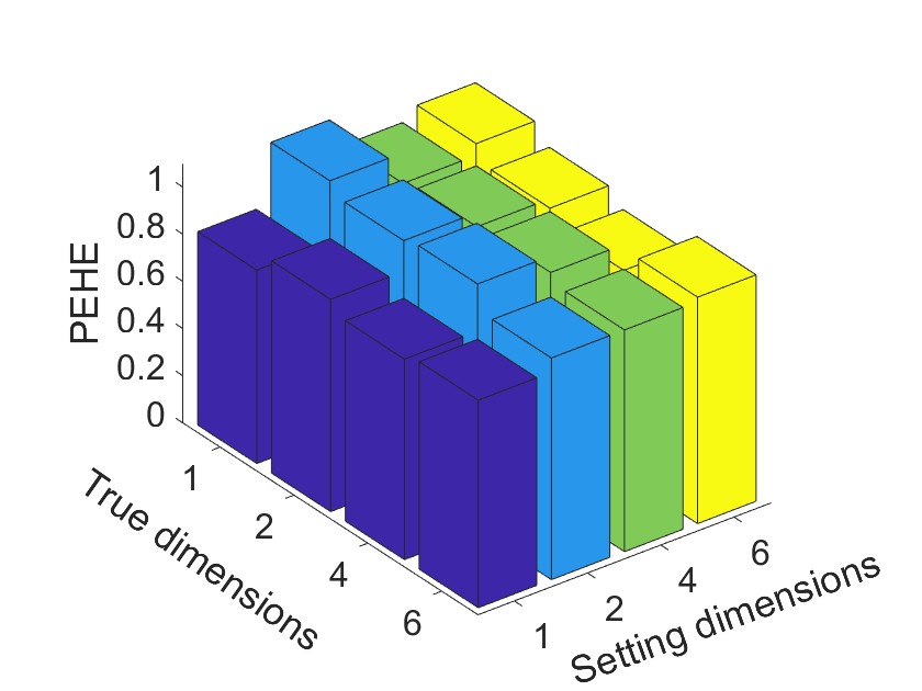
There are two representations and in our study and we set their dimensions to 1 for both. To demonstrate the effectiveness of this setting, we conduct experiments on datasets with samples fixed at 10k and repeat the experiments independently 30 times to minimize random noise for each setting. We generate a set of simulation datasets based on the data generation process described in Section 5.2, setting the dimensions of the two latent variables to , respectively. In our CPTiVAE algorithm, we conduct experiments with the two parameters set to respectively.
Figure 2 shows the AE and PEHE of the CPTiVAE algorithm on these datasets. When is set to regardless of the true dimensions of and , the CPTiVAE algorithm obtains the smallest AE and PEHE on the synthetic datasets. Furthermore, our experiments demonstrate that the CPTiVAE algorithm is effective in addressing high-dimensional latent variables. Hence, it is reasonable to set and to 1.
5.5 Experiments on Semi-Synthetic Datasets
In this section, we compare our CPTiVAE algorithm with the baseline methods on the semi-synthetic dataset based on the IHDP dataset. The Infant Health and Development Program (IHDP) is a randomized controlled study designed to evaluate the effect of physician home visits on infants’ cognitive scores. The IHDP dataset is often used as a baseline dataset to evaluate causal effect methods [49]. The dataset contains 747 samples and 25 variables, and in our experiments, following the synthetic dataset generation process described in Section 5.2, two post-treatment variables were generated based on these 25 variables.
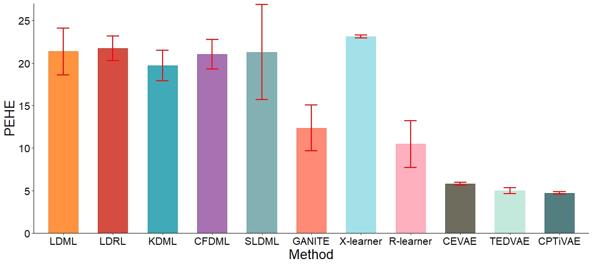
The performance of the CPTiVAE algorithm on semi-synthetic datasets is shown in Figure 3. We observe that the CPTiVAE algorithm achieves the smallest AE and PEHE. This further illustrates that the CPTiVAE algorithm can effectively tackle both latent confounders and post-treatment variables.
5.6 Case Study on a Real-World Dataset
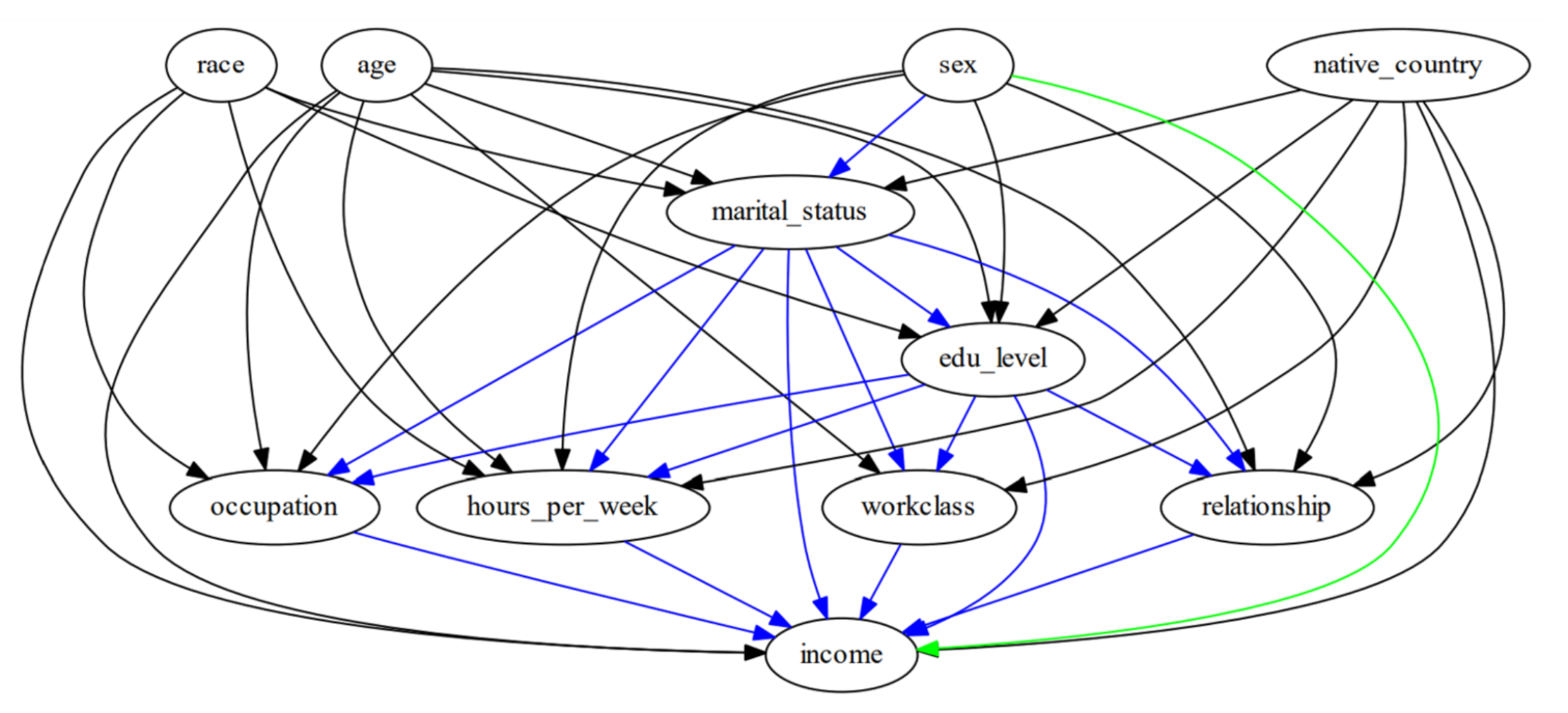
In this section, we apply the CPTiVAE algorithm to study the causal effect of education level on income in the Adult dataset [51]. The Adult dataset contains 14 attributes for 48,842 individuals, which is retrieved from the UCI repositiry [52]. In our problem setting, some extraneous variables, such as sex, relationship, and race, are not relevant to our study, and we remove these variables. For convenience, we divide the years of education into 2 groups, those greater than 10 years as the treatment group and the rest as the control group. We define education-num as , income as , age and marital status as , and the remaining attributes as , including workclass, occupation, and hours-per-week.
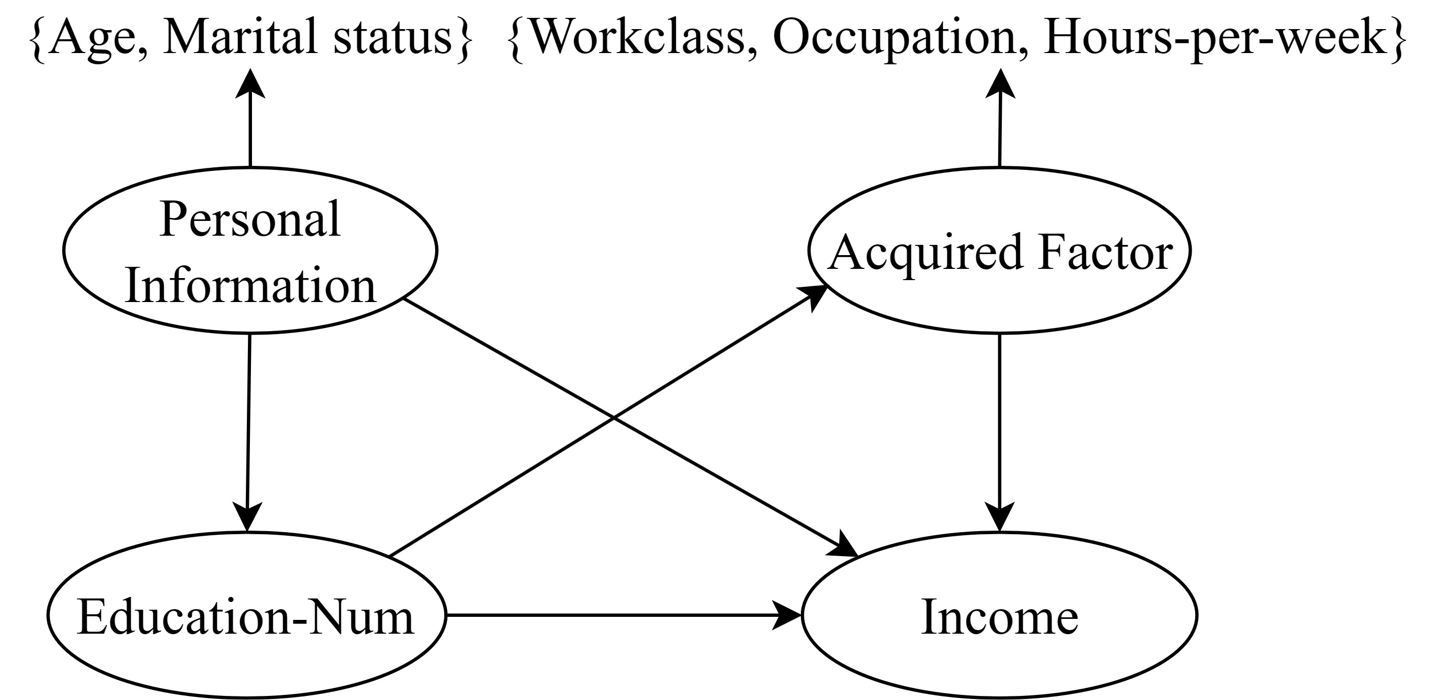
The causal network for the Adult dataset is shown in 4. Based on the complete causal DAG, we can obtain the simplified DAG in Figure 5, and aim to estimate the causal effect of education level on income. In this example, we consider the proxy of acquired factors to be accessible, and they are workclass, occupation, and hours-per-week.
We obtain by using the CPTiVAE algorithm, which is consistent with the conclusion that education has a positive effect on income [53]. In contrast, we obtain if all covariates are defined as , and if only considering the latent confounders. Both indicate that education level has no or marginal effects on income which is not the correct conclusion. This shows that if we do not consider , the causal effect estimation will be biased.
6 Conclusion
In this paper, we address the challenging problem of estimating causal effects from observational data with latent confounders and post-treatment variables. We propose the use of the VAE and the identifiable VAE techniques for learning the representations of latent confounders and post-treatment variables, respectively. Furthermore, we provide theoretical proof for the identifiability in terms of the learned representation . Extensive experiments on synthetic and semi-synthetic datasets demonstrate that CPTiVAE outperforms existing methods for ATE and CATE estimation. We also examine that CPTiVAE’s performance remains robust against variations in the model parameters and . Additionally, a case study on the real-world dataset further illustrates CPTiVAE’s potential in practical scenarios.
References
- [1] G. W. Imbens and D. B. Rubin, Causal Inference for Statistics, Social, and Biomedical Sciences: An Introduction. Cambridge University Press, 2015.
- [2] D. B. Rubin, “Causal inference using potential outcomes: Design, modeling, decisions,” Journal of the American Statistical Association, vol. 100, no. 469, pp. 322–331, 2005.
- [3] F. D. Johansson, U. Shalit, et al., “Learning representations for counterfactual inference,” ArXiv, 2018.
- [4] J. Connors, Alfred F. and S. et al, “The effectiveness of right heart catheterization in the initial care of critically iii patients,” Journal of the American Medical Association, vol. 276, no. 11, pp. 889–897, 1996.
- [5] R. Guo, L. Cheng, J. Li, et al., “A survey of learning causality with data,” ACM Computing Surveys, vol. 53, no. 4, pp. 1–37, 2020.
- [6] A. Deaton and N. Cartwright, “Understanding and misunderstanding randomized controlled trials,” Social Science and Medicine, vol. 210, pp. 2–21, 2018.
- [7] D. Cheng, J. Li, L. Liu, et al., “Data-driven causal effect estimation based on graphical causal modelling: A survey,” ACM Computing Surveys, vol. 56, no. 5, pp. 1–37, 2022.
- [8] L. Yao, Z. Chu, S. Li, et al., “A survey on causal inference,” ACM Transactions on Knowledge Discovery from Data, vol. 15, no. 5, pp. 1–46, 2021.
- [9] J. Pearl, Causality. Cambridge University Press, 2 ed., 2009.
- [10] S. Athey, J. Tibshirani, and S. Wager, “Generalized random forests,” The Annals of Statistics, vol. 47, no. 2, pp. 1148 – 1178, 2019.
- [11] A. Acharya, M. Blackwell, and M. Sen, “Explaining causal findings without bias: Detecting and assessing direct effects,” American Political Science Review, vol. 110, no. 3, pp. 512–529, 2016.
- [12] S. J. Pocock, S. Assmann, L. E. Enos, et al., “Subgroup analysis, covariate adjustment and baseline comparisons in clinical trial reporting: current practiceand problems,” Statistics in Medicine, vol. 21, pp. 2917–2930, 2002.
- [13] K. L. M. Fan Li and A. M. Zaslavsky, “Balancing covariates via propensity score weighting,” Journal of the American Statistical Association, vol. 113, no. 521, pp. 390–400, 2018.
- [14] S. Athey and G. Imbens, “Recursive partitioning for heterogeneous causal effects,” Proceedings of the National Academy of Sciences, vol. 113, no. 27, pp. 7353–7360, 2016.
- [15] X. Su, C.-L. Tsai, H. Wang, et al., “Subgroup analysis via recursive partitioning.,” Journal of Machine Learning Research, vol. 10, no. 2, pp. 1–18, 2009.
- [16] U. Shalit, F. D. Johansson, and D. Sontag, “Estimating individual treatment effect: generalization bounds and algorithms,” in International conference on machine learning, pp. 3076–3085, 2017.
- [17] J. Yoon, J. Jordon, and M. Van Der Schaar, “Ganite: Estimation of individualized treatment effects using generative adversarial nets,” in International conference on learning representations, pp. 1–22, 2018.
- [18] N. Kallus, “Deepmatch: Balancing deep covariate representations for causal inference using adversarial training,” in International Conference on Machine Learning, pp. 5067–5077, 2020.
- [19] C. Louizos, U. Shalit, et al., “Causal effect inference with deep latent-variable models,” Advances in neural information processing systems, vol. 30, pp. 1–12, 2017.
- [20] W. Miao, Z. Geng, and E. T. Tchetgen, “Identifying causal effects with proxy variables of an unmeasured confounder,” Biometrika, vol. 105, no. 4, pp. 987–993, 2018.
- [21] J. M. Wooldridge, “On estimating firm-level production functions using proxy variables to control for unobservables,” Economics Letters, vol. 104, pp. 112–114, 2009.
- [22] Z. Xu, D. Cheng, J. Li, J. Liu, L. Liu, and K. Wang, “Disentangled representation for causal mediation analysis,” in Proceedings of the AAAI Conference on Artificial Intelligence, pp. 10666–10674, 2023.
- [23] Z. Xu, D. Cheng, J. Li, J. Liu, L. Liu, and K. Yu, “Causal inference with conditional front-door adjustment and identifiable variational autoencoder,” in The Twelfth International Conference on Learning Representations, 2023.
- [24] W. Zhang, L. Liu, and J. Li, “Treatment effect estimation with disentangled latent factors,” in Proceedings of the AAAI Conference on Artificial Intelligence, vol. 35, pp. 10923–10930, 2021.
- [25] I. Higgins, L. Matthey, A. Pal, et al., “beta-vae: Learning basic visual concepts with a constrained variational framework,” in International conference on learning representations, pp. 1–22, 2016.
- [26] H. Kim and A. Mnih, “Disentangling by factorising,” in International Conference on Machine Learning, pp. 2649–2658, 2018.
- [27] R. Lopez, J. Regier, M. I. Jordan, et al., “Information constraints on auto-encoding variational bayes,” Advances in neural information processing systems, vol. 31, pp. 1–12, 2018.
- [28] O. Rybkin, K. Daniilidis, and S. Levine, “Simple and effective vae training with calibrated decoders,” in International Conference on Machine Learning, pp. 9179–9189, 2021.
- [29] Z. Kuang, F. Sala, N. Sohoni, et al., “Ivy: Instrumental variable synthesis for causal inference,” in International Conference on Artificial Intelligence and Statistics, pp. 398–410, 2020.
- [30] R. Singh, M. Sahani, and A. Gretton, “Kernel instrumental variable regression,” Advances in Neural Information Processing Systems, vol. 32, pp. 1–13, 2019.
- [31] K. Muandet, A. Mehrjou, S. K. Lee, and A. Raj, “Dual instrumental variable regression,” Advances in Neural Information Processing Systems, vol. 33, pp. 2710–2721, 2020.
- [32] P. Spirtes, C. N. Glymour, R. Scheines, et al., Causation, Prediction, and Search. MIT Press, 2000.
- [33] P. R. Rosenbaum and D. B. Rubin, “The central role of the propensity score in observational studies for causal effects,” Biometrika, vol. 70, no. 1, pp. 41–55, 1983.
- [34] D. B. Rubin, “Using multivariate matched sampling and regression adjustment to control bias in observational studies,” Journal of the American Statistical Association, vol. 74, no. 366a, pp. 318–328, 1979.
- [35] X. De Luna, I. Waernbaum, and T. S. Richardson, “Covariate selection for the nonparametric estimation of an average treatment effect,” Biometrika, vol. 98, no. 4, pp. 861–875, 2011.
- [36] E. Perkovi, J. Textor, M. Kalisch, et al., “Complete graphical characterization and construction of adjustment sets in markov equivalence classes of ancestral graphs,” Journal of Machine Learning Research, vol. 18, no. 220, pp. 1–62, 2018.
- [37] J. M. Montgomery, B. Nyhan, and M. Torres, “How conditioning on posttreatment variables can ruin your experiment and what to do about it,” American Journal of Political Science, vol. 62, pp. 760–775, 2018.
- [38] I. Khemakhem, D. P. Kingma, and A. Hyvärinen, “Variational autoencoders and nonlinear ica: A unifying framework,” in International Conference on Artificial Intelligence and Statistics, pp. 1–10, 2019.
- [39] D. P. Kingma and M. Welling, “Auto-encoding variational bayes,” in 2nd International Conference on Learning Representations, 2014.
- [40] R. Cai, W. Chen, Z. Yang, et al., “Long-term causal effects estimation via latent surrogates representation learning,” ArXiv, 2022.
- [41] V. Chernozhukov, D. Chetverikov, M. Demirer, et al., “Double/debiased machine learning for treatment and structural parameters,” The Econometrics Journal, vol. 21, no. 1, pp. 1–68, 2018.
- [42] D. J. Foster and V. Syrgkanis, “Orthogonal statistical learning,” The Annals of Statistics, vol. 51, no. 3, pp. 879–908, 2023.
- [43] X. Nie and S. Wager, “Quasi-oracle estimation of heterogeneous treatment effects,” Biometrika, vol. 108, no. 2, pp. 299–319, 2021.
- [44] V. Semenova, M. Goldman, V. Chernozhukov, et al., “Estimation and inference on heterogeneous treatment effects in high-dimensional dynamic panels,” ArXiv: Machine Learning, pp. 1 – 40, 2017.
- [45] S. R. Künzel, J. S. Sekhon, P. J. Bickel, et al., “Metalearners for estimating heterogeneous treatment effects using machine learning,” Proceedings of the national academy of sciences, vol. 116, no. 10, pp. 4156–4165, 2019.
- [46] A. Paszke, S. Gross, F. Massa, et al., “Pytorch: An imperative style, high-performance deep learning library,” Advances in neural information processing systems, vol. 32, pp. 1–12, 2019.
- [47] E. Bingham, J. P. Chen, et al., “Pyro: Deep universal probabilistic programming,” The Journal of Machine Learning Research, vol. 20, no. 1, pp. 973–978, 2019.
- [48] Y. Zhao and Q. Liu, “Causal ml: Python package for causal inference machine learning,” SoftwareX, vol. 21, p. 101294, 2023.
- [49] J. L. Hill, “Bayesian nonparametric modeling for causal inference,” Journal of Computational and Graphical Statistics, vol. 20, no. 1, pp. 217–240, 2011.
- [50] L. Zhang, Y. Wu, and X. Wu, “A causal framework for discovering and removing direct and indirect discrimination,” in Proceedings of the Twenty-Sixth International Joint Conference on Artificial Intelligence, IJCAI-17, pp. 3929–3935, 2017.
- [51] J. Li, S. Ma, T. Le, et al., “Causal decision trees,” IEEE Transactions on Knowledge and Data Engineering, vol. 29, no. 2, pp. 257–271, 2017.
- [52] D. Dua and C. Graff, “Uci machine learning repository.” http://archive.ics.uci.edu/ml, 2017.
- [53] Y. Hu, Y. Wu, L. Zhang, et al., “A generative adversarial framework for bounding confounded causal effects,” Proceedings of the AAAI Conference on Artificial Intelligence, vol. 35, no. 13, pp. 12104–12112, 2021.