Lifting MGARD: construction of (pre)wavelets on the interval using polynomial predictors of arbitrary order

Abstract

MGARD (MultiGrid Adaptive Reduction of Data) is an algorithm for compressing and refactoring scientific data, based on the theory of multigrid methods. The core algorithm is built around stable multilevel decompositions of conforming piecewise linear $C^{0}$ finite element spaces, enabling accurate error control in various norms and derived quantities of interest. In this work, we extend this construction to arbitrary order Lagrange finite elements $\mathbb{Q}_{p}$, $p\geq 0$, and propose a reformulation of the algorithm as a lifting scheme with polynomial predictors of arbitrary order. Additionally, a new formulation using a compactly supported wavelet basis is discussed, and an explicit construction of the proposed wavelet transform for uniform dyadic grids is described.

Viktor Reshniak${}^{{\href mailto:reshniakv@ornl.gov}*1}$, Evan Ferguson${}^{{\href mailto:efergu2@uw.edu}2}$, Qian Gong${}^{{\href mailto:gongq@ornl.gov}1}$,

Nicolas Vidal${}^{{\href mailto:vidaln@ornl.gov}1}$, Rick Archibald${}^{{\href mailto:archibaldrk@ornl.gov}1}$ and Scott Klasky${}^{{\href mailto:klasky@ornl.gov}1}$

¹Oak Ridge National Laboratory, Oak Ridge, TN, USA

²University of Washington, Seattle, Washington, USA

1 Introduction

Compression of scientific data is known to be particularly challenging as it is widely regarded as effectively incompressible due to the intrinsically high entropy of its floating-point value representation [30, 22]. Lossless compressors achieve at most mediocre performance on such datasets [38]. At the same time, scientific data from simulations and experiments is often inherently lossy and can tolerate some error-controlled loss in its accuracy. Wavelets are particularly appealing for this task because of their excellent localization properties in both spatial and frequency domains [32].

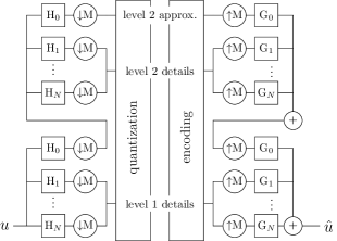
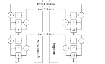
Wavelet compression is closely related to the time-scale multiresolution analysis which is rooted in Laplacian pyramids [8], hierarchical filters [29, 36], multirate and polyphase filter banks [35, 15, 14], see Figure 1. Conventional wavelets are constructed with translation invariant filters defined on regular nested dyadic grids. Invertibility, smoothness, vanishing moments, and the support size of the wavelet basis functions are the main design criteria commonly imposed in the frequency domain for such regularly sampled signals.

c0ptt-12pt c0ptt-12pt

Figure 1: Schematic illustration of the two-level decomposition/recomposition of a signal using equivalent subband coding filter bank (left) and lifting scheme (right) implementations.

Lifting provides an alternative approach for constructing wavelets directly in the signal domain using appropriate linear combinations of scaling functions [33]. The scheme comprises the split/merge, predict, and update operations and is invertible by design. After the signal is split into two components, the values in one are used to predict the values of another, and the prediction error is recorded as the detail coefficients, see Figure 1. The quality of predictor is largely responsible for the energy compaction of this decomposition while the update operation is commonly designed to match the vanishing moments of the primal/reconstruction and dual/analysis wavelets, the property generally leading to better stability of the wavelet transform. Factorization of classical wavelet decompositions into lifting steps also provides more efficient implementation over the filter bank construction [11]. As a result, lifting is used as a coding algorithm in wavelet-based compressors including JPEG2000 [34] and SPECK [27] for size-bounded compression, Waverange [21] and SPERR [24] for error-controlled compression of structured scientific data, and HexaShrink [28] for compression of structured hexahedral volume meshes.

On a more abstract note, the construction of wavelets is intricately tied to the concept of stable decomposition of function spaces. Considering a family of projectors $\mathcal{P}_{j}:V\to V_{j}$ with $V_{j}\subset V_{j+1}\subset V$ and $\mathcal{P}_{j}\mathcal{P}_{j+1}=\mathcal{P}_{j}$, an element $u\in V$ possesses a multiscale representation

$$u=\sum_{j=0}^{\infty}(\mathcal{P}_{j}-\mathcal{P}_{j-1})u=\mathcal{P}_{0}u+\sum_{j=0}^{\infty}\mathcal{Q}_{j}u,\qquad\mathcal{Q}_{j}=\mathcal{P}_{j+1}-\mathcal{P}_{j}:V\to W_{j}.$$ (1)

The projector $\mathcal{Q}_{j}$ is also a projector since $\mathcal{Q}_{j}^{2}=\mathcal{P}_{j+1}^{2}-\mathcal{P}_{j+1}\mathcal{P}_{j}-\mathcal{P}_{j}\mathcal{P}_{j+1}+\mathcal{P}_{j}^{2}=\mathcal{P}_{j+1}-\mathcal{P}_{j}$. Consequently, since $\mathcal{P}_{j}(\mathcal{P}_{j+1}-\mathcal{P}_{j})=0$, the element $\mathcal{Q}_{j}u\in W_{j}$ can be viewed as the detail complement of $\mathcal{P}_{j}u\in V_{j}$ in $V_{j+1}$ leading to the direct sum decomposition of the space $V$

$$V=V_{0}\bigoplus_{l=0}^{\infty}W_{l}.$$

The choice of appropriate projectors is crucial to obtain decompositions with certain desirable properties such as, e.g., the polynomial exactness of $V_{j}$ or the stability of the representation (1) written in terms of the bases of the approximation and detail subspaces $V_{j}:=span\{\varphi_{j,k}:k\in\Delta_{j}\}$, $W_{j}:=span\{\psi_{j,k}:k\in\nabla_{j}\}$

$$u =\sum_{k\in\Delta_{0}}\alpha_{0,k}\varphi_{0,k}+\sum_{j\geq 0}\sum_{k\in\nabla_{j}}\beta_{j,k}\psi_{j,k}\qquad\text{s.t.}\quad\|u\|_{V}\sim\vvvert\boldsymbol{\alpha}\cup\boldsymbol{\beta}\vvvert,$$ (2)

where $\vvvert\cdot\vvvert$ is a corresponding discrete norm and $\|\cdot\|\sim\vvvert\cdot\vvvert$ denotes the usual norm equivalence, i.e., the existence of finite constants $\gamma,\Gamma$ with $\gamma\vvvert\boldsymbol{\alpha}\cup\boldsymbol{\beta}\vvvert\leq\|u\|_{V}\leq\Gamma\vvvert\boldsymbol{\alpha}\cup\boldsymbol{\beta}\vvvert.$

In the case of $V$ being a Hilbert space, a suitable candidate for $\mathcal{P}_{j}$ is an oblique projector defined as

$$\mathcal{P}_{j}u=\sum_{k\in\Delta_{j}}\langle u,\tilde{\varphi}_{j,k}\rangle\varphi_{j,k},$$ (3)

where $\tilde{\varphi}$ is biorthogonal to $\varphi$, i.e., $\langle\varphi_{j,k},\tilde{\varphi}_{l,k^{\prime}}\rangle=\delta_{k,k^{\prime}}$. It has been shown that biorthogonality is a necessary condition for the uniform stability of multiscale representations in the sense of the norm equivalence in (2) when $V$ is $L^{2}$ [10, 9]. This condition eliminates the selection of interpolation operators

$$\mathcal{I}_{j}u=\sum_{k\in\Delta_{j}}u_{k}\varphi_{j,k},\qquad[\varphi_{j,k}]_{k^{\prime}}=\delta_{k,k^{\prime}},$$ (4)

as uniformly $L^{2}$-stable projectors, given that $\tilde{\varphi}_{j,k}$ is a Dirac distribution defined by $\langle u,\tilde{\varphi}_{j,k}\rangle:=u_{j,k}$. In terms of the lifting scheme, this corresponds to the interpolating predictor without an update operation, underscoring once again the significance of the update operation in achieving stable multiresolution encoding.

Similar results also hold in $L^{p}$-Besov spaces $V:=B^{t}_{p,q}$ as given by

Theorem 1.1 ([9, Theorem 3.7.7]).

Assume that $\varphi,\tilde{\varphi}$ are compactly supported biorthogonal scaling functions with $\varphi\in L^{r}$, $\tilde{\varphi}\in L^{r^{\prime}}$ for $r\in[1,\infty]$, $1/r+1/r^{\prime}=1$, or that $\varphi\in C^{0}$ and $\tilde{\varphi}$ is a Radon measure in which case $r=\infty$. Then, for $0<p\leq r$, one has the norm equivalence

$$\|u\|_{B^{s}_{p,q}}\sim\|\mathcal{P}_{0}u\|_{L^{p}}+\left\|\left\{2^{sj}\|\mathcal{Q}_{j}u\|_{L^{p}}:j\geq 0\right\}\right\|_{l^{q}},$$

for all $s>0$ such that

$$d\left(\frac{1}{p}-\frac{1}{r}\right)<s<\min(t,n+1),$$ (5)

where $n$ is the order of polynomial reproduction in $V_{j}$ and $t$ is such that $\varphi\in B^{t}_{p,q_{0}}$ for some $q_{0}$.

The condition in (5) defines the valid range of the smoothness of the space in which the norm is assessed. This range is characterized by the data dimensionality $d$, smoothness $t$ and polynomial reproduction $n$ of the basis $\varphi$, and $L^{r}$ stability of the projector in (3). Since $B^{s}_{2,2}=H^{s}$, Theorem 1.1 is also immediately valid for the usual Sobolev spaces $H^{s}$ which, together with the $L^{2}$ stability result, gives

$$\|u\|_{H^{s}}^{2}\sim\sum_{k\in\Delta_{0}}|\alpha_{k}|^{2}+\sum_{j\geq 0}\sum_{k\in\nabla_{j}}2^{2sj}|\beta_{j,k}|^{2},\quad d\left(\frac{1}{2}-\frac{1}{r}\right)\leq s<\min(t,n+1).$$ (6)

Such norm equivalences in $H^{s}$ have been extensively studied in the design of additive multilevel preconditioners of elliptic operators [37, 7, 26].

For piecewise polynomial nodal basis, it can be shown that $\varphi\in H^{t}$ with $t<n+1/2$, where $n$ is the order of the basis. This simplifies the upper bound in (6). To simplify the lower bound, we need $r=2$ to get rid of the dimension $d$ yielding

$$\varphi\text{ is }n\text{-th order Lagrange polynomial }\quad\to\quad 0\leq s<n+1/2.$$

It is also worth noting that Theorem 1.1 allows using interpolation projectors in (4) that are $L^{p}$ unstable for all $p<\infty$. However, the condition in (6) becomes more restrictive due to its dependence on the dimension $d$. For instance, the piecewise linear interpolation corresponds to $n=1$, $r=\infty$, and $\varphi\in H^{3/2}$ resulting in $s\in\left(\frac{d}{2},\frac{3}{2}\right)$ if $d\leq 2$ and no valid values for $d>2$. These lower bounds once again highlight the special role of $L^{2}$-stable projectors.

MGARD (MultiGrid Adaptive Reduction of Data) is an error controlled compression algorithm that builds upon the theory of stable decomposition of function spaces discussed above [2, 3, 17, 18]. The main ingredient of MGARD is given by $L^{2}$-orthogonal projectors that we denote $\mathcal{P}_{j}^{o}$ to make a distinction from the more general oblique projectors $\mathcal{P}_{j}$ in (3). The apparent drawback of this approach is the global support of the dual basis $\tilde{\varphi}$. However, it is partially eliminated by efficient linear-complexity solvers for inverting banded Gramm matrices of compactly supported primal basis $\varphi$ in one-dimensional and tensor-product spaces. Using the equivalence relation in (6), MGARD is capable to control the compression error in the corresponding Sobolev norms, as well as in $L^{\infty}$ norm and arbitrary linear quantities of interest (QoI) [4]. Further extensions include machine learning assisted error control of nonlinear QoI [23], adaptive compression with feature preservation [19], and compression of data defined on certain unstructured grids [5].

The core MGARD algorithm is designed assuming piecewise linear data representation. As a result, the norm equivalence in (6) is valid only for $s\in[0,3/2)$ and the method cannot take advantage of higher regularity in data. In this work, we extend this construction to arbitrary order Lagrange finite elements $Q_{p}$, $p\geq 0$, and propose a reformulation of the algorithm as a lifting scheme with variable order polynomial predictors.

The paper is organized as follows. In Section 2, we formulate MGARD transform as a lifting scheme, provide its matrix formulation, and describe refinement equations. Section 3 is devoted to the specific construction for the uniform dyadic grids on the interval and tensor product grids. Section 4 contains numerical results demonstrating properties of the transform. Section 5 concludes the discussion and provides several directions for future work.

2 MGARD wavelet transform

Here we provide a rather general construction of MGARD transform as a wavelet lifting scheme. First, denote by $V(\Omega)$ the space of continuous functions defined on a compact set $\Omega\in\mathbb{R}^{d}$ and consider a sequence of nested grids

$$\mathcal{G}_{0}\subset\ldots\subset\mathcal{G}_{j-1}\subset\mathcal{G}_{j}\subset\ldots\subset\mathcal{G}_{L}\subset\Omega,\qquad\mathcal{G}_{j}:=\{x_{k}:k\in\Delta_{j}\},$$

for some nested nodal index sets $\Delta_{j-1}\subset\Delta_{j}$. For each grid $\mathcal{G}_{j}$, consider two subdivisions into

• a collection $\mathcal{T}_{j}$ of non-overlapping elements,

• a collection $\mathcal{S}_{j}$ of non-overlapping subdomains such that each $\sigma\in\mathcal{S}_{j}$ is a union of one or more connected elements in $\mathcal{T}_{j}$. A natural choice for $\mathcal{S}_{j}$ is $\mathcal{T}_{k},\;k\leq j$.

Figure 2 illustrates one possible subdivision of the grid in two domains.

Figure 2: A subdivision of two domains into elements $\mathcal{T}$ (gray) and subdomains $\mathcal{S}$ (black).

Denote by $\Delta^{\tau}_{j}:=\Delta_{j}\cap\tau$, i.e., those indices of $\Delta_{j}$ that are also in $\tau\in\mathcal{T}_{j}$. Define $\Delta^{\sigma}_{j}:=\Delta_{j}\cap\sigma$ analogously. To each $\sigma\in\mathcal{S}_{j}$, associate a discrete function space $V_{j}^{\sigma}$ with a nodal basis $\{\varphi^{\sigma}_{j,k}:k\in\Delta^{\sigma}_{j}\}$. Given $V_{j}^{\sigma}$, define two function spaces on the whole grid $\mathcal{G}_{j}$:

• a ‘broken’ space $V_{\mathcal{S}_{j}}:=\bigoplus_{\sigma\in\mathcal{S}_{j}}V^{\sigma}_{j}$ of functions that are continuous in each $\sigma\in\mathcal{S}_{j}$, but discontinuous across the subdomains,

• a space $V_{j}$ of continuous functions spanned by the global nodal basis $\{\varphi_{j,k}:k\in\Delta_{j}\}$, i.e., the basis of $V_{\mathcal{S}_{j}}$ except the basis vectors at the interface nodes are ‘glued’ together.

Remark 1.

For the proposed construction, one needs to ensure the nestedness of the spaces $V_{j}\subset V_{j+1}$ and $V_{\mathcal{S}_{j}}\subset V_{\mathcal{S}_{j+1}}$. In one dimension, the natural choice is the space of piecewise polynomials on dyadically refined grids. In this scenario, each polynomial on the coarse element is precisely represented by two polynomials of the same order on the elements of the finer grid. This construction is also applicable to tensor product spaces. A similar approach applies to certain simplicial meshes obtained through iterative refinement of the initial mesh via subdivision of simplex edges [5], see Figure 2. Consequently, the data values at the nodes of the coarsest simplex uniquely determine the linear function that can be exactly represented by simplexes at finer levels. However, this method does not straightforwardly extend to general unstructured meshes. One potential solution involves commencing with the final mesh and employing mesh coarsening to establish the mesh hierarchy. The function spaces on the resulting polygonal meshes can then be defined by employing generalized barycentric coordinates, augmented with additional constraints to ensure hierarchical construction [16, 20].

Given a sequence of nested spaces $V_{j}$, consider three projection operators:

1. the interpolation operator $\mathcal{I}_{j}:V\to V_{j}$

   $$\mathcal{I}_{j}u=\sum_{k\in\Delta_{j}}u_{k}\varphi_{j,k},$$ (7)

2. the family of (oblique) projectors $\mathcal{P}_{j}:=\mathcal{A}_{\mathcal{S}_{j}}\mathcal{P}_{\mathcal{S}_{j}}:V\to V_{j}$ with the projectors $\mathcal{P}_{\mathcal{S}_{j}}:V\to V_{\mathcal{S}_{j}}$ defined in each subdomain as

   $$(\mathcal{P}_{\mathcal{S}_{j}}u,v)_{\sigma} =(u,v)_{\sigma},\quad\forall u\in V,v\in V^{\sigma}_{j},$$ (8)

   and the operator $\mathcal{A}_{\mathcal{S}_{j}}:V_{\mathcal{S}_{j}}\to V_{j}$ used to enforce the nodal continuity at the interface nodes

   $$\mathcal{A}_{\mathcal{S}_{j}}u =\sum_{k\in\Delta_{j}}\{\!\{u_{k}\}\!\}\varphi_{j,k},$$ (9)

   where $\{\!\{u_{k}\}\!\}$ is the average value, and

3. the detail projection operator $\mathcal{Q}_{j}:=\mathcal{P}_{j+1}-\mathcal{P}_{j}:V\to W_{j}$ inducing the orthogonal decomposition of each $V_{j}$ into its approximation and detail subspaces $V_{j}=V_{j-1}\oplus W_{j-1}$.

Note that when $S_{j}$ consists of the single subdomain, $\mathcal{P}_{j}$ is the $L^{2}$-orthogonal projector onto $V_{j}$. We will denote such a projector as $\mathcal{P}_{j}^{cg}$ to emphasize its relation to the continuous Galerkin finite element approximation. Similarly, we will use $\mathcal{P}_{j}^{dg}$ to denote the projector in (8)-(9) when $\mathcal{S}_{j}=\mathcal{T}_{j}$. Figure 3 shows different projections into the space of piecewise quadratic functions defined on the grid with eight elements.

Figure 3: Projections into the space of piecewise polynomials on the grid with $2^{3}$ elements.

The crux of the MGARD wavelet transform is based on the following factorizations of $\mathcal{P}_{j}$ and $\mathcal{Q}_{j}$

$$\mathcal{P}_{j} =\mathcal{I}_{j}\mathcal{P}_{j+1}+(\mathcal{P}_{j}-\mathcal{I}_{j}\mathcal{P}_{j+1})=\Big{(}\mathcal{I}_{j}+\mathcal{P}_{j}(I-\mathcal{I}_{j})\Big{)}\mathcal{P}_{j+1},$$ (10)

$$\mathcal{Q}_{j} :=\mathcal{P}_{j+1}-\mathcal{P}_{j}=\Big{(}I-\mathcal{I}_{j}-\mathcal{P}_{j}(I-\mathcal{I}_{j})\Big{)}\mathcal{P}_{j+1}=\big{(}I-\mathcal{P}_{j}\big{)}\big{(}I-\mathcal{I}_{j}\big{)}\mathcal{P}_{j+1},$$ (11)

where we used $\mathcal{P}_{j}\mathcal{I}_{j}=\mathcal{I}_{j}$ which trivially holds for the projectors in (7) and (8)-(9).

For any $v\in V_{j+1}$, we have $(v-\mathcal{I}_{j}v)\in V_{j+1}$ with

$$v-\mathcal{I}_{j}v=\sum_{k\in\nabla_{j}}\big{[}v-\mathcal{I}_{j}v\big{]}_{k}\varphi_{j+1,k},$$

and hence

$$\big{(}I-\mathcal{P}_{j}\big{)}\big{(}I-\mathcal{I}_{j}\big{)}\sum_{k\in\Delta_{j+1}}v_{k}\varphi_{j+1,k}=\sum_{k\in\nabla_{j}}\big{[}v-\mathcal{I}_{j}v\big{]}_{k}\big{(}I-\mathcal{P}_{j}\big{)}\varphi_{j+1,k},$$

where $\nabla_{j}:=\Delta_{j+1}\setminus\Delta_{j}$ is the surplus index set of those indices in $\Delta_{j+1}$ that are not in $\Delta_{j}$. It is convenient to write the above representation of $\mathcal{Q}_{j}v\in W_{j}$ for any $v\in V_{j+1}$ as an expansion

$$\mathcal{Q}_{j}v:=\big{(}I-\mathcal{P}_{j}\big{)}\big{(}I-\mathcal{I}_{j}\big{)}v=\sum_{k\in\nabla_{j}}\beta_{j,k}\psi_{j,k}$$ (12)

with

$$\beta_{j,k} :=\big{[}v-\mathcal{I}_{j}v\big{]}_{k},\qquad\psi_{j,k}:=\big{(}I-\mathcal{P}_{j}\big{)}\varphi_{j+1,k},\qquad k\in\nabla_{j}.$$ (13)

Hence, $\psi_{j,k}$ is the basis of the detail subpace $W_{j}$, and the wavelet coefficients $\beta_{j,k}$ quantify the mismatch between $v\in V_{j+1}$ and its interpolant $\mathcal{I}_{j}v\in V_{j}$ at the surplus nodes of $\nabla_{j}$. By this definition, the coefficients $\beta_{j,k}$ are identically zero for all $v\in V_{j}$. Analogously, $\mathcal{P}_{j}\psi_{j,k}=0$ by construction reflecting the orthogonality of spaces $V_{j}\perp W_{j}$.

Similarly to (12), one gets

$$\mathcal{P}_{j}v :=\Big{(}\mathcal{I}_{j}+\mathcal{P}_{j}(I-\mathcal{I}_{j})\Big{)}\sum_{k\in\Delta_{j+1}}v_{k}\varphi_{j+1,k}=\sum_{k\in\Delta_{j}}v_{k}\varphi_{j,k}+\sum_{n\in\nabla_{j}}\beta_{j,n}\mathcal{P}_{j}\varphi_{j+1,n}$$ (14)

$$=\sum_{k\in\Delta_{j}}v_{k}\varphi_{j,k}+\sum_{n\in\nabla_{j}}\beta_{j,n}\sum_{k\in\Delta_{j}}u_{j,k,n}\varphi_{j,k}=\sum_{k\in\Delta_{j}}\left(v_{k}+\sum_{n\in\nabla_{j}}u_{j,k,n}\beta_{j,n}\right)\varphi_{j,k},$$

where $\{u_{j,k,n}:k\in\nabla_{j}\}$ are the coefficients in the nodal basis expansion of

$$\mathcal{P}_{j}\varphi_{j+1,n}=\sum_{k\in\Delta_{j}}u_{j,k,n}\varphi_{j,k},\quad n\in\nabla_{j}.$$ (15)

We now have all the components to formulate MGARD transform as a lifting scheme using the Split, Predict and Update operations detailed below.

Split operation. Denote by $\boldsymbol{\alpha}_{j+1}:=\{[\mathcal{P}_{j+1}u]_{k}:k\in\Delta_{j+1}\}$ the vector of the nodal values of $\mathcal{P}_{j+1}v\in V_{j+1}$ at $\Delta_{j+1}$. Given $\boldsymbol{\alpha}_{j+1}$, the Split operation produces two vectors with the values of $\mathcal{P}_{j+1}v$ at the nodes of $\Delta_{j}\subset\Delta_{j+1}$ and $\nabla_{j}\subset\Delta_{j+1}$, namely $\boldsymbol{\alpha}_{j+1}^{\Delta}:=\{[\mathcal{P}_{j+1}v]_{k}:k\in\Delta_{j}\}$ and $\boldsymbol{\alpha}_{j+1}^{\nabla}:=\{[\mathcal{P}_{j+1}v]_{k}:k\in\nabla_{j}\}$.

Predict operation. Using the nodal values of $\mathcal{P}_{j+1}v$ at $\Delta_{j}$, the Predict operation estimates the values of $\mathcal{P}_{j+1}v$ at the nodes of $\nabla_{j}$ using the interpolant in (7). The detail coefficients are then calculated as the mismatch of this prediction

$$\boldsymbol{\beta}_{j}=\boldsymbol{\alpha}_{j+1}^{\nabla}-\mathbf{P}_{j}\boldsymbol{\alpha}_{j+1}^{\Delta},$$

where $\boldsymbol{\beta}_{j}:=\{\beta_{j,k}:k\in\nabla_{j}\}$, and $\mathbf{P}_{j}\in\mathbb{R}^{|\nabla_{j}^{\sigma}|\times|\Delta_{j}^{\sigma}|}$ is the matrix representation of the interpolating predictor.

Update operation. Given the nodal values $\boldsymbol{\alpha}_{j+1}^{\Delta}$ of $\mathcal{P}_{j+1}v$ at $\Delta_{j}$ and the detail coefficients $\boldsymbol{\beta}_{j}$ at $\nabla_{j}$, the Update operation calculates the nodal values $\boldsymbol{\alpha}_{j}$ of $\mathcal{P}_{j}v$ at $\Delta_{j}$ using (14). Specifically, the coefficients $\mathbf{U}^{\sigma}_{j}:=\{u^{\sigma}_{j,k,n}:k\in\Delta^{\sigma}_{j},n\in\nabla^{\sigma}_{j}\}$ for the projections of the basis functions $\{\varphi^{\sigma}_{j+1,n}:n\in\nabla^{\sigma}_{j}\}$ in each subdomain $\sigma\in\mathcal{S}_{j}$ are given by

$$\mathbf{G}_{\scriptscriptstyle\Delta_{j}\Delta_{j}}^{\sigma}\mathbf{U}^{\sigma}_{j}=\mathbf{G}_{\scriptscriptstyle\Delta_{j}\nabla_{j}}^{\sigma}\quad\to\quad\mathbf{U}^{\sigma}_{j}=\left(\mathbf{G}_{\scriptscriptstyle\Delta_{j}\Delta_{j}}^{\sigma}\right)^{-1}\mathbf{G}_{\scriptscriptstyle\Delta_{j}\nabla_{j}}^{\sigma},$$ (16)

where $\mathbf{G}_{\scriptscriptstyle\Delta_{j}\Delta_{j}}^{\sigma}$ and $\mathbf{G}_{\scriptscriptstyle\Delta_{j}\nabla_{j}}^{\sigma}$ are the Gram matrices with the entries

$$[\mathbf{G}_{\scriptscriptstyle\Delta_{j}\Delta_{j}}^{\sigma}]_{n^{\prime},m^{\prime}}:=\langle\varphi^{\sigma}_{j,n},\varphi^{\sigma}_{j,m}\rangle,\quad n\in\Delta^{\sigma}_{j},m\in\Delta^{\sigma}_{j},$$

$$[\mathbf{G}_{\scriptscriptstyle\Delta_{j}\nabla_{j}}^{\sigma}]_{n^{\prime},m^{\prime}}:=\langle\varphi^{\sigma}_{j,n},\varphi^{\sigma}_{j+1,m}\rangle,\quad n\in\Delta^{\sigma}_{j},m\in\nabla^{\sigma}_{j},$$

and $n^{\prime},m^{\prime}$ are the local (to the subdomain $\sigma$) indices of the global indices $n,m$. The columns of the update matrix $\mathbf{U}^{\sigma}_{j}\in\mathbb{R}^{|\Delta_{j}^{\sigma}|\times|\nabla_{j}^{\sigma}|}$ contain the nodal values of the projected basis functions in each subdomain. The global update matrix $\mathbf{U}_{j}\in\mathbb{R}^{|\Delta_{j}|\times|\nabla_{j}|}$ is then obtained by applying the averaging operator in (9) to the columns of $\{\mathbf{U}^{\sigma}_{j},\sigma\in\mathcal{S}_{j}\}$.

Consequently, the nodal values $\boldsymbol{\alpha}_{j}$ of $\mathcal{P}_{j}u$ at $\Delta_{j}$ are calculated as

$$\boldsymbol{\alpha}_{j}=\boldsymbol{\alpha}_{j+1}^{\Delta}+\mathbf{U}_{j}\boldsymbol{\beta}_{j}.$$

The steps in the described transform are fully invertible, as indicated in Figure 4, with the obvious definition of the Merge operation. To summarize, the steps for the forward and inverse transforms are given in Table 1.

c0ptt-12pt

Figure 4: Schematic illustration of MGARD lifting steps.

Forward transform, $\mathsf{MGARD}_{j+1\to j}:\boldsymbol{{\alpha}}_{j+1}\to(\boldsymbol{{\alpha}}_{j},\boldsymbol{{\beta}}_{j})$			Inverse transform, $\mathsf{MGARD}_{j\to j+1}^{-1}:(\boldsymbol{{\alpha}}_{j},\boldsymbol{{\beta}}_{j})\to\boldsymbol{{\alpha}}_{j+1}$
$\displaystyle\boldsymbol{{\alpha}}_{j+1}^{\Delta},\boldsymbol{{\alpha}}_{j+1}^{\nabla}$ $\displaystyle=\text{{Split}}(\boldsymbol{{\alpha}}_{j+1})$ (17) $\displaystyle\boldsymbol{{\beta}}_{j}$ $\displaystyle=\boldsymbol{{\alpha}}_{j+1}^{\nabla}-\mathbf{P}_{j}\boldsymbol{{\alpha}}_{j+1}^{\Delta}$ (18) $\displaystyle\boldsymbol{{\alpha}}_{j}$ $\displaystyle=\boldsymbol{{\alpha}}_{j+1}^{\Delta}+\mathbf{U}_{j}\boldsymbol{{\beta}}_{j}$ (19)			$\displaystyle\boldsymbol{{\alpha}}_{j+1}^{\Delta}$ $\displaystyle=\boldsymbol{{\alpha}}_{j}-\mathbf{U}_{j}\boldsymbol{{\beta}}_{j}$ (20) $\displaystyle\boldsymbol{\alpha}_{j+1}^{\nabla}$ $\displaystyle=\boldsymbol{{\beta}}_{j}+\mathbf{P}_{j}\boldsymbol{{\alpha}}_{j+1}^{\Delta}$ (21) $\displaystyle\boldsymbol{{\alpha}}_{j+1}$ $\displaystyle=\text{{Merge}}(\boldsymbol{{\alpha}}_{j+1}^{\Delta},\boldsymbol{{\alpha}}_{j+1}^{\nabla})$ (22)

Table 1: MGARD transform steps.

Remark 2.

It is important to highlight that the factorizations in (10)-(11) remain valid for any pair of projectors satisfying $\mathcal{P}_{j}\mathcal{I}_{j}=\mathcal{I}_{j}$. For example, if we substitute $\mathcal{P}_{j}$ with $\mathcal{I}_{j}$, we recover the hierarchical basis construction of Yserentant in [7]. However, such replacement lacks stability, as indicated in Section 1. On a positive note, this substitution leads to a straightforward implementation since the Update operation is not required. The advantage of introducing the interpolation operator $\mathcal{I}_{j}$ into the factorizations of $\mathcal{P}_{j}$ and $\mathcal{Q}_{j}$ becomes apparent from the expansions in (12), (14) which require the same number of degrees of freedom in total as the original projector $\mathcal{P}_{j+1}$. Additionally, the nodal basis used in (7) enables a straightforward interpretation of data as the coefficients of such basis expansions.

2.1 Matrix formulation

The following definitions are helpful to formulate the matrix representation of the transform.

Definition 2.1.

Define two binary operations:

1. $\blackdiamond:\mathbb{R}^{\mathord{\mathchoice{\vbox{\hbox{\scalebox{0.7}{$\displaystyle\bullet$}}}}{\vbox{\hbox{\scalebox{0.7}{$\textstyle\bullet$}}}}{\vbox{\hbox{\scalebox{0.7}{$\scriptstyle\bullet$}}}}{\vbox{\hbox{\scalebox{0.7}{$\scriptscriptstyle\bullet$}}}}}\times\Delta_{j}}\times\mathbb{R}^{\mathord{\mathchoice{\vbox{\hbox{\scalebox{0.7}{$\displaystyle\bullet$}}}}{\vbox{\hbox{\scalebox{0.7}{$\textstyle\bullet$}}}}{\vbox{\hbox{\scalebox{0.7}{$\scriptstyle\bullet$}}}}{\vbox{\hbox{\scalebox{0.7}{$\scriptscriptstyle\bullet$}}}}}\times\nabla_{j}}\to\mathbb{R}^{\mathord{\mathchoice{\vbox{\hbox{\scalebox{0.7}{$\displaystyle\bullet$}}}}{\vbox{\hbox{\scalebox{0.7}{$\textstyle\bullet$}}}}{\vbox{\hbox{\scalebox{0.7}{$\scriptstyle\bullet$}}}}{\vbox{\hbox{\scalebox{0.7}{$\scriptscriptstyle\bullet$}}}}}\times\Delta_{j+1}}$ creates a new matrix by merging the columns of the inputs according to the index sets $\Delta_{j},\nabla_{j}\subset\Delta_{j+1}$,

2. $\diamond:\mathbb{R}^{\Delta_{j}\times\mathord{\mathchoice{\vbox{\hbox{\scalebox{0.7}{$\displaystyle\bullet$}}}}{\vbox{\hbox{\scalebox{0.7}{$\textstyle\bullet$}}}}{\vbox{\hbox{\scalebox{0.7}{$\scriptstyle\bullet$}}}}{\vbox{\hbox{\scalebox{0.7}{$\scriptscriptstyle\bullet$}}}}}}\times\mathbb{R}^{\nabla_{j}\times\mathord{\mathchoice{\vbox{\hbox{\scalebox{0.7}{$\displaystyle\bullet$}}}}{\vbox{\hbox{\scalebox{0.7}{$\textstyle\bullet$}}}}{\vbox{\hbox{\scalebox{0.7}{$\scriptstyle\bullet$}}}}{\vbox{\hbox{\scalebox{0.7}{$\scriptscriptstyle\bullet$}}}}}}\to\mathbb{R}^{\Delta_{j+1}\times\mathord{\mathchoice{\vbox{\hbox{\scalebox{0.7}{$\displaystyle\bullet$}}}}{\vbox{\hbox{\scalebox{0.7}{$\textstyle\bullet$}}}}{\vbox{\hbox{\scalebox{0.7}{$\scriptstyle\bullet$}}}}{\vbox{\hbox{\scalebox{0.7}{$\scriptscriptstyle\bullet$}}}}}}$ creates a new matrix by merging the rows of the inputs according to the index sets $\Delta_{j},\nabla_{j}\subset\Delta_{j+1}$.

The following properties are trivial

1. $\mathbf{c}(\mathbf{a}\blackdiamond\mathbf{b})=\mathbf{c}\mathbf{a}\blackdiamond\mathbf{c}\mathbf{b}$,

2. $(\mathbf{a}\diamond\mathbf{b})\mathbf{c}=\mathbf{a}\mathbf{c}\diamond\mathbf{b}\mathbf{c}$,

3. $(\mathbf{a}\blackdiamond\mathbf{b})(\mathbf{c}\diamond\mathbf{d})=\mathbf{a}\mathbf{c}+\mathbf{b}\mathbf{d}$,

4. $[\mathbf{a},\mathbf{b}]^{T}\blackdiamond[\mathbf{c},\mathbf{d}]^{T}=[\mathbf{a}\blackdiamond\mathbf{c},\mathbf{b}\blackdiamond\mathbf{d}]^{T}$,

5. $[\mathbf{a},\mathbf{b}]\diamond[\mathbf{c},\mathbf{d}]=[\mathbf{a}\diamond\mathbf{c},\mathbf{b}\diamond\mathbf{d}]$,

6. $(\mathbf{a}\blackdiamond\mathbf{b})^{T}=\mathbf{a}^{T}\diamond\mathbf{b}^{T}$.

7. $\mathbf{a}\diamond(\mathbf{b}+\mathbf{c})=\mathbf{a}\diamond\mathbf{b}+\mathbf{a}\diamond\mathbf{c}$

8. $(\mathbf{a}+\mathbf{b})\blackdiamond\mathbf{c}=\mathbf{a}\blackdiamond\mathbf{c}+\mathbf{b}\blackdiamond\mathbf{c}$

Definition 2.2.

For any two matrices $\mathbf{a}\in\mathbb{R}^{m\times n}$, $\mathbf{b}\in\mathbb{R}^{p\times q}$, define the following concatenation operators

$$\mathbf{a}\binrel@{\ominus}\binrel@@{\vphantom{\ominus}\mathchoice{\smash{\makebox[9.99997pt]{\rotatebox[origin={c}]{90.0}{$\displaystyle\ominus$}}}}{\smash{\makebox[9.99997pt]{\rotatebox[origin={c}]{90.0}{$\textstyle\ominus$}}}}{\smash{\makebox[7.66663pt]{\rotatebox[origin={c}]{90.0}{$\scriptstyle\ominus$}}}}{\smash{\makebox[6.11107pt]{\rotatebox[origin={c}]{90.0}{$\scriptscriptstyle\ominus$}}}}} :=\begin{bmatrix}a_{00}&\ldots&a_{0n}&&\\ \vdots&\ddots&\vdots&&\\ a_{m0}&\ldots&a_{mn}&&\\ &&b_{00}&\ldots&b_{0q}\\ &&\vdots&\ddots&\vdots\\ &&b_{p0}&\ldots&b_{pq}\\ \end{bmatrix},\qquad \mathbf{a}\ominus\mathbf{b}:=\begin{bmatrix}a_{00}&\ldots&a_{0n}&&&\\ \vdots&\ddots&\vdots&&&\\ a_{m0}&\ldots&a_{mn}&b_{00}&\ldots&b_{0q}\\ &&&\vdots&\ddots&\vdots\\ &&&b_{p0}&\ldots&b_{pq}\\ \end{bmatrix},$$

$$\mathbf{a}\oplus\mathbf{b} :=\begin{bmatrix}a_{00}&\ldots&a_{0n}&&\\ \vdots&\ddots&\vdots&&\\ a_{m0}&\ldots&a_{mn}+b_{00}&\ldots&b_{0q}\\ &&\vdots&\ddots&\vdots\\ &&b_{p0}&\ldots&b_{pq}\\ \end{bmatrix},\qquad \mathbf{a}\binrel@{\oslash}\binrel@@{\mathchoice{\reflectbox{$\displaystyle\oslash$}}{\reflectbox{$\textstyle\oslash$}}{\reflectbox{$\scriptstyle\oslash$}}{\reflectbox{$\scriptscriptstyle\oslash$}}}\mathbf{b}:=\begin{bmatrix}a_{00}&\ldots&a_{0n}&&&\\ \vdots&\ddots&\vdots&&&\\ a_{m0}&\ldots&a_{mn}&&&\\ &&&b_{00}&\ldots&b_{0q}\\ &&&\vdots&\ddots&\vdots\\ &&&b_{p0}&\ldots&b_{pq}\\ \end{bmatrix},$$

so that $\mathbf{a}\binrel@{\ominus}\binrel@@{\vphantom{\ominus}\mathchoice{\smash{\makebox[9.99997pt]{\rotatebox[origin={c}]{90.0}{$\displaystyle\ominus$}}}}{\smash{\makebox[9.99997pt]{\rotatebox[origin={c}]{90.0}{$\textstyle\ominus$}}}}{\smash{\makebox[7.66663pt]{\rotatebox[origin={c}]{90.0}{$\scriptstyle\ominus$}}}}{\smash{\makebox[6.11107pt]{\rotatebox[origin={c}]{90.0}{$\scriptscriptstyle\ominus$}}}}}\mathbf{b}\in\mathbb{R}^{m+p\times n+q-1}$, $\mathbf{a}\ominus\mathbf{b}\in\mathbb{R}^{m+p-1\times n+q}$, $\mathbf{a}\oplus\mathbf{b}\in\mathbb{R}^{m+p-1\times n+q-1}$, and $\mathbf{a}\binrel@{\oslash}\binrel@@{\mathchoice{\reflectbox{$\displaystyle\oslash$}}{\reflectbox{$\textstyle\oslash$}}{\reflectbox{$\scriptstyle\oslash$}}{\reflectbox{$\scriptscriptstyle\oslash$}}}\mathbf{b}\in\mathbb{R}^{m+p\times n+q}$.

Using Definition 2.1, the matrix representations of the transform are given by

$$\begin{bmatrix}\boldsymbol{{\alpha}}_{j}\\[5.0pt] \boldsymbol{{\beta}}_{j}\end{bmatrix} =\mathsf{M}_{j}\cdot\boldsymbol{{\alpha}}_{j+1},\qquad\boldsymbol{{\alpha}}_{j+1}=\mathsf{M}_{j}^{-1}\cdot\begin{bmatrix}\boldsymbol{{\alpha}}_{j}\\[5.0pt] \boldsymbol{{\beta}}_{j}\end{bmatrix},$$ (23)

where

$$\mathsf{M}_{j} :=\begin{bmatrix}[r]\mathsf{A}_{j}\\[5.0pt] \mathsf{B}_{j}\end{bmatrix},\qquad\mathsf{M}_{j}^{-1}:=\begin{bmatrix}\mathsf{C}_{j}&\mathsf{D}_{j}\end{bmatrix}$$

with

$$\mathsf{A}_{j} :=\big{(}\mathbf{I}_{\scriptscriptstyle{\Delta_{j}}}-\mathbf{U}_{j}\mathbf{P}_{j}\big{)}\blackdiamond\mathbf{U}_{j},\quad \mathsf{B}_{j}:=(-\mathbf{P}_{j})\blackdiamond\mathbf{I}_{\scriptscriptstyle{\nabla_{j}}},$$

$$\mathsf{C}_{j} :=\mathbf{I}_{\scriptscriptstyle{\Delta_{j}}}\diamond\mathbf{P}_{j},\qquad \mathsf{D}_{j}:=(-\mathbf{U}_{j})\diamond(\mathbf{I}_{\scriptscriptstyle{\nabla_{j}}}-\mathbf{P}_{j}\mathbf{U}_{j}),$$

and $\mathbf{I}_{\scriptscriptstyle{\Delta_{j}}},\mathbf{I}_{\scriptscriptstyle{\nabla_{j}}}$ are the identity matrices of the appropriate size.

For the composite transform, we have

$$\begin{bmatrix}\boldsymbol{{\alpha}}_{0}\\ \boldsymbol{{\beta}}_{0}\\ \vdots\\ \boldsymbol{{\beta}}_{J-1}\end{bmatrix}=\mathsf{M}\cdot\boldsymbol{{\alpha}}_{J}=\prod_{j=0}^{J-1}\begin{bmatrix}[r]\mathsf{M}_{j}&\\ &\mathbf{I}_{\scriptscriptstyle{|\Delta_{J}|-|\Delta_{j}|}}\end{bmatrix}\cdot\boldsymbol{{\alpha}}_{J},$$ (24)

and similarly for the inverse transform

$$\boldsymbol{{\alpha}}_{J} =\mathsf{M}^{-1}\cdot\boldsymbol{{\alpha}}_{J}=\prod_{j=1}^{J}\begin{bmatrix}\mathsf{M}_{J-j}^{-1}&\\ &\mathbf{I}_{\scriptscriptstyle{|\Delta_{J}|-|\Delta_{j}|}}\end{bmatrix}\begin{bmatrix}\boldsymbol{{\alpha}}_{0}\\ \boldsymbol{{\beta}}_{0}\\ \vdots\\ \boldsymbol{{\beta}}_{J-1}\end{bmatrix},$$ (25)

where $\mathsf{M}$ is the transform matrix.

2.2 Refinement equations

2.2.1 Primal basis

Given the inverse transform $\mathsf{MGARD}_{j\to j+1}^{-1}$, one immediately gets the refinement equations for the nodal and wavelet bases. Specifically, the transform $\mathsf{MGARD}_{j\to j+1}^{-1}(\boldsymbol{{\delta}}^{\scriptscriptstyle\Delta_{j}}_{k},\boldsymbol{{0}})=\text{{Merge}}(\boldsymbol{{\delta}}^{\scriptscriptstyle\Delta_{j}}_{k},\mathbf{P}_{j}\boldsymbol{{\delta}}^{\scriptscriptstyle\Delta_{j}}_{k})$ gives the refinement equation for the nodal basis

$$\varphi_{j,k} =\varphi_{j+1,k}+\sum_{p\in\nabla_{j}}[\mathbf{P}_{j}]_{p,k}\varphi_{j+1,p},\qquad k\in\Delta_{j},$$ (26)

where $\boldsymbol{{\delta}}^{\scriptscriptstyle\Delta_{j}}_{k}$ is the standard basis vector on $\Delta_{j}$ with the unit element in the $k$-th position. Similarly, the refinement equation for the wavelet basis is given by $\mathsf{MGARD}_{j+1\to j}^{-1}(\boldsymbol{{0}},\boldsymbol{{\delta}}^{\scriptscriptstyle\nabla_{j}}_{k})=\text{{Merge}}(-\mathbf{U}_{j}\boldsymbol{{\delta}}^{\scriptscriptstyle\nabla_{j}}_{k},(\mathbf{I}_{\scriptscriptstyle{\nabla_{j}}}-\mathbf{P}_{j}\mathbf{U}_{j})\boldsymbol{{\delta}}^{\scriptscriptstyle\nabla_{j}}_{k})$

$$\psi_{j,k} =\varphi_{j+1,k}-\sum_{p\in\Delta_{j}}[\mathbf{U}_{j}]_{p,k}\varphi_{j+1,p}-\sum_{p\in\nabla_{j}}[\mathbf{P}_{j}\mathbf{U}_{j}]_{p,k}\varphi_{j+1,p}\qquad k\in\nabla_{j}.$$ (27)

One can use (26) to simplify the above expression as

$$\psi_{j,k} =\varphi_{j+1,k}-\sum_{p\in\Delta_{j}}[\mathbf{U}_{j}]_{p,k}\varphi_{j+1,p}-\sum_{n\in\Delta_{j}}[\mathbf{U}_{j}]_{n,k}(\varphi_{j,n}-\varphi_{j+1,n})$$

$$=\varphi_{j+1,k}-\sum_{p\in\Delta_{j}}[\mathbf{U}_{j}]_{p,k}\varphi_{j,p}.$$

In the vector-matrix form, the refinement equations in (26)-(27) are written as

$$\boldsymbol{{\varphi}}_{j} =\boldsymbol{{\varphi}}_{j+1}\cdot\mathsf{C}_{j},$$ (28)

$$\boldsymbol{{\psi}}_{j} =\boldsymbol{{\varphi}}_{j+1}\cdot\mathsf{D}_{j},$$ (29)

where $\boldsymbol{{\varphi}}_{j}:=\{\varphi_{j,k}:k\in\Delta_{j}\}$, $\boldsymbol{{\psi}}_{j}:=\{\psi_{j,k}:k\in\nabla_{j}\}$ are the row vectors of basis functions. The refinement equation (28) is somewhat redundant as the nodal basis at each level is fixed a-priory.

Recurrent application of the above formulas gives the so-called cascade algorithm that implicitly defines the basis functions at any point in the domain. Specifically, equations (28)-(29) involve the same matrices as the matrix form of the inverse transform. The nodal representation of the basis vectors at any level $J$ is then given by the columns of the matrices in (25) as

$$\boldsymbol{{\varphi}}_{j} =\boldsymbol{{\varphi}}_{J}\cdot\left(\prod_{l=j+1}^{J-1}\mathsf{C}_{J+j-l}\right)\cdot\mathsf{C}_{j},$$ (30)

$$\boldsymbol{{\psi}}_{j} =\boldsymbol{{\varphi}}_{J}\cdot\left(\prod_{l=j+1}^{J-1}\mathsf{C}_{J+j-l}\right)\cdot\mathsf{D}_{j}.$$ (31)

2.2.2 Dual basis

In order to determine the values of the dual basis functions $\tilde{\boldsymbol{{\varphi}}}$, $\tilde{\boldsymbol{{\psi}}}$, one can use the definition of the wavelet coefficients in the expansion

$$P_{j}u=\sum_{k\in\Delta_{j}}\alpha_{j,k}\varphi_{j,k}+\sum_{l\geq j}\sum_{k\in\nabla_{l}}\beta_{l,k}\psi_{l,k}=\sum_{k\in\Delta_{j}}\langle u,\tilde{\varphi}_{j,k}\rangle\varphi_{j,k}+\sum_{l\geq j}\sum_{k\in\nabla_{l}}\langle u,\tilde{\psi}_{l,k}\rangle\psi_{l,k}.$$

When $u:=\delta(\cdot-y)$ is the Dirac measure centered at $y$, we get $\tilde{\psi}_{j,k}(y):=\langle\delta(\cdot-y),\tilde{\psi}_{j,k}\rangle$. Hence, the coefficients of the above expansion provide the values of the dual basis functions at a given point. These values are given by the forward MGARD transform $(\tilde{\boldsymbol{{\varphi}}}_{j},\tilde{\boldsymbol{{\psi}}}_{j})_{p}=\mathsf{MGARD}_{J\to j}(\varepsilon_{J,p}^{-1}\boldsymbol{{\delta}}_{p}^{\scriptscriptstyle\Delta_{J}})$. The scaling $\varepsilon_{J,p}^{-1}$ of the standard basis vector $\boldsymbol{{\delta}}_{p}^{\scriptscriptstyle\Delta_{J}}$ ensures the unit integral of the approximate delta function at the level $J$ and is required for the weak convergence to the Dirac distribution when $J\to\infty$. The nodal representation of the dual basis vectors $\tilde{\boldsymbol{{\varphi}}},\tilde{\boldsymbol{{\psi}}}$ at the nodes of $\Delta_{J}$ is thus given by

$$\tilde{\boldsymbol{{\varphi}}}_{j} =\mathsf{A}_{j}\cdot\Bigg{(}\prod_{l=j+1}^{J-1}\mathsf{A}_{l}\Bigg{)}\cdot\boldsymbol{{\varepsilon}}_{J}^{-1}\cdot\boldsymbol{{\varphi}}_{J}^{T},$$ (32)

$$\tilde{\boldsymbol{{\psi}}}_{j} =\mathsf{B}_{j}\cdot\Bigg{(}\prod_{l=j+1}^{J-1}\mathsf{A}_{l}\Bigg{)}\cdot\boldsymbol{{\varepsilon}}_{J}^{-1}\cdot\boldsymbol{{\varphi}}_{J}^{T},$$ (33)

where $\tilde{\boldsymbol{{\varphi}}}_{j}:=\{\tilde{\varphi}_{j,k}:k\in\Delta_{j}\}$, $\tilde{\boldsymbol{{\psi}}}_{j}:=\{\tilde{\psi}_{j,k}:k\in\nabla_{j}\}$ are the column vectors of dual basis functions, and $\boldsymbol{{\varepsilon}}_{J}^{-1}:=\operatorname{diag}\big{(}\{\varepsilon_{J,k}^{-1}:k\in\Delta_{J}\}\big{)}$ is the diagonal scaling matrix.

By comparing the expressions for $\tilde{\boldsymbol{{\varphi}}}_{j}$, $\tilde{\boldsymbol{{\varphi}}}_{j-1}$, one gets the refinement equations for the dual basis as well

$$\tilde{\boldsymbol{{\varphi}}}_{j} =\mathsf{A}_{j}\cdot\tilde{\boldsymbol{{\varphi}}}_{j+1},$$ (34)

$$\tilde{\boldsymbol{{\psi}}}_{j} =\mathsf{B}_{j}\cdot\tilde{\boldsymbol{{\varphi}}}_{j+1},$$ (35)

with

$$\tilde{\boldsymbol{{\varphi}}}_{J-1} =\mathsf{A}_{J-1}\cdot\boldsymbol{{\varepsilon}}_{J}^{-1}\cdot\boldsymbol{{\varphi}}_{J}^{T},$$ (36)

$$\tilde{\boldsymbol{{\psi}}}_{J-1} =\mathsf{B}_{J-1}\cdot\boldsymbol{{\varepsilon}}_{J}^{-1}\cdot\boldsymbol{{\varphi}}_{J}^{T}.$$ (37)

Similarly to (26)-(27), we can write the refinement equations for each basis vector as

$$\tilde{\psi}_{j,k} =\tilde{\varphi}_{j+1,k}-\sum_{p\in\Delta_{j}}[\mathbf{P}_{j}]_{k,p}\tilde{\varphi}_{j+1,p},\quad k\in\nabla_{j},$$ (38)

$$\tilde{\varphi}_{j,k} =\tilde{\varphi}_{j+1,k}+\sum_{p\in\nabla_{j}}[\mathbf{U}_{j}]_{k,p}\tilde{\psi}_{j,p},\phantom{{}_{+1}}\quad k\in\Delta_{j}.$$ (39)

3 Uniform dyadic grids on $\Omega:=[0,1]$

c0ptt-12pt

Figure 5: One-dimensional coarse (solid) and surplus (dashed) Lagrange basis functions at two adjacent grid levels $\mathcal{G}_{c/f}$. The corresponding one-dimensional elements $\tau_{c/f}^{q}$ and grid spacings $h_{c/f}$ are also shown.

The above results are valid for any choice of the nodal basis for the nested spaces $V_{j}\subset V_{j+1}$. Here we focus on the particular case of the piecewise polynomial basis on dyadically refined uniform grids of the unit interval in one dimension.

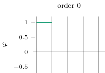
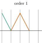
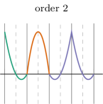
Without loss of generality, consider a two-level decomposition scheme for the coarse and fine grids $\mathcal{G}_{j}\subset\mathcal{G}_{j+1}$. Define a 1D element $\tau\in\mathcal{T}_{j}$ of order $q>0$ as a collection of $q+1$ consecutive nodes of the corresponding grid. The element of order $q=0$ is defined using the cádlág (right continuous with left limit) nodal basis function, see Figure 5 for the illustration. Each grid $\mathcal{G}_{j}$ has $2^{j}$ elements, and we assume that $\mathcal{G}_{0}$ has $q+1$ nodes. We also use the primed indices to denote the local-to-the-element numbering of nodes, e.g., $p^{\prime}\in[0,\ldots,q]\leftrightarrow p\in\Delta_{j}^{\tau}$. Finally, $\tau_{k}$ denotes the element that contains the node with index $k$.

In this case, one has

$$\mathbf{P}_{j}=\underbrace{\mathbf{P}^{q}\binrel@{\ominus}\binrel@@{\vphantom{\ominus}\mathchoice{\smash{\makebox[9.99997pt]{\rotatebox[origin={c}]{90.0}{$\displaystyle\ominus$}}}}{\smash{\makebox[9.99997pt]{\rotatebox[origin={c}]{90.0}{$\textstyle\ominus$}}}}{\smash{\makebox[7.66663pt]{\rotatebox[origin={c}]{90.0}{$\scriptstyle\ominus$}}}}{\smash{\makebox[6.11107pt]{\rotatebox[origin={c}]{90.0}{$\scriptscriptstyle\ominus$}}}}}\ldots\binrel@{\ominus}\binrel@@{\vphantom{\ominus}\mathchoice{\smash{\makebox[9.99997pt]{\rotatebox[origin={c}]{90.0}{$\displaystyle\ominus$}}}}{\smash{\makebox[9.99997pt]{\rotatebox[origin={c}]{90.0}{$\textstyle\ominus$}}}}{\smash{\makebox[7.66663pt]{\rotatebox[origin={c}]{90.0}{$\scriptstyle\ominus$}}}}{\smash{\makebox[6.11107pt]{\rotatebox[origin={c}]{90.0}{$\scriptscriptstyle\ominus$}}}}}\mathbf{P}^{q}}_{2^{j}\text{ times}},$$

with the $q$-order interpolation matrix $\mathbf{P}^{q}\in\mathbb{R}^{q\times(q+1)}$ defined in Appendix A.1. The refinement equations involving the interpolation matrix then simplify to

$$\varphi_{j,k} =\varphi_{j+1,k}+\sum_{p\in\nabla_{j}}[\mathbf{P}_{j}]_{p,k}\varphi_{j+1,p}=\varphi_{j+1,k}+\sum_{p\in\nabla_{j}^{\tau_{k}}}[\mathbf{P}^{q}]_{p^{\prime},k^{\prime}}\varphi_{j+1,p}\quad k\in\Delta_{j},$$

$$\tilde{\psi}_{j,k} =\tilde{\varphi}_{j+1,k}-\sum_{p\in\Delta_{j}}[\mathbf{P}_{j}]_{k,p}\tilde{\varphi}_{j+1,p}=\tilde{\varphi}_{j+1,k}-\sum_{p\in\Delta_{j}^{\tau_{k}}}[\mathbf{P}^{q}]_{k^{\prime},p^{\prime}}\tilde{\varphi}_{j+1,p},\quad k\in\nabla_{j}.$$

3.0.1 Normalization

The $L^{2}$ norms of the one-dimensional basis functions can be calculated exactly using the Newton-Cotes quadratures since each $\varphi_{j,k}$ is a compactly supported piecewise polynomial. This gives

$$\|\varphi_{j,k}\|^{2} :=\sum_{\tau\in\mathcal{T}_{j}}\int_{\tau}\varphi_{j,k}^{2}dx=2^{-j}\sum_{\tau\in\mathcal{T}_{j}}\sum_{p\in\Delta_{j+1}^{\tau}}w_{p^{\prime}}\big{[}\mathsf{C}_{j}]_{p,k}^{2},$$ (40)

$$\|\psi_{j,k}\|^{2} :=\sum_{\tau\in\mathcal{T}_{j}}\int_{\tau}\psi_{j,k}^{2}dx=2^{-j}\sum_{\tau\in\mathcal{T}_{j}}\sum_{p\in\Delta_{j+1}^{\tau}}w_{p^{\prime}}\big{[}\mathsf{D}_{j}]_{p,k}^{2},$$ (41)

where $2^{-j}$ is the length of the element of the grid $\mathcal{G}_{j}$. The quadrature weights $w_{p^{\prime}}$ can be found, e.g., in [1, 31]. Since each $\varphi_{j,k}$ is supported on at most two elements, for the indices $k$ inside the element, we have

$$\|\varphi_{j,k}\|^{2}=\int_{\tau_{k}}\varphi_{j,k}^{2}dx=2^{-j}\Big{(}w_{k^{\prime}}+\sum_{p^{\prime}=0}^{q-1}w_{2p^{\prime}+1}\big{[}\mathbf{P}^{q}]_{p^{\prime},k^{\prime}}^{2}\Big{)}.$$ (42)

Similarly, for the boundary nodes shared between the elements, we get

$$\|\varphi_{j,k^{\prime}}\|^{2}=2^{1-j}\Big{(}w_{0}+\sum_{p^{\prime}=0}^{q-1}w_{2p^{\prime}+1}\big{[}\mathbf{P}^{q}]_{p^{\prime},k^{\prime}}^{2}\Big{)}.$$ (43)

3.0.2 Interpolating projectors

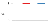
Figure 6: The primal and dual basis functions induced by $\mathcal{P}_{j}=\mathcal{I}_{j}$ at level $1$. For clarity, only one basis vector per element is shown for the dual wavelet basis $\tilde{\psi}$.

For the case of interpolating basis with $\mathcal{P}_{j}=\mathcal{I}_{j}$, one gets $\mathbf{U}_{j}=\boldsymbol{{0}}$ which simplifies the refinement equations (26)-(27), (38)-(39) yielding

$$\boldsymbol{{\varphi}}_{j} =\Big{\{}\varphi_{j,k}:k\in\Delta_{j}\Big{\}},\qquad\boldsymbol{{\psi}}_{j}=\Big{\{}\varphi_{j+1,k}:k\in\nabla_{j}\Big{\}}.$$

So the approximation basis is just the nodal basis of the grid at level $j$ while the wavelet basis consists of the next-level nodal basis vectors at the surplus nodes in $\nabla_{j}$.

For the dual bases, one gets

$$\tilde{\boldsymbol{{\varphi}}}_{j} =\Big{\{}\tilde{\varphi}_{j+1,k}:k\in\Delta_{j}\Big{\}}=\Big{\{}2^{J}\varphi_{J,k}:k\in\Delta_{j}\Big{\}}\xrightarrow{J\to\infty}\Big{\{}\delta(\cdot-x_{k}):k\in\Delta_{j}\Big{\}},$$

$$\tilde{\boldsymbol{{\psi}}}_{j} =\Big{\{}\tilde{\varphi}_{j+1,k}-\sum_{p\in\Delta_{j}^{\tau_{k}}}[\mathbf{P}^{q}]_{k^{\prime},p^{\prime}}\tilde{\varphi}_{j+1,p}:k\in\nabla_{j}\Big{\}}$$

$$\xrightarrow{J\to\infty}\Big{\{}\delta(\cdot-x_{k})-\sum_{p\in\Delta_{j}^{\tau_{k}}}[\mathbf{P}^{q}]_{k^{\prime},p^{\prime}}\delta\big{(}\cdot-x_{p}\big{)}:k\in\nabla_{j}\Big{\}}.$$

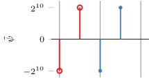
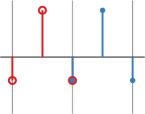
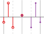
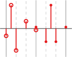
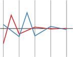
Hence, the dual approximation basis vectors are the Dirac measures centered at the nodes of $\Delta_{j}$. The dual wavelet vectors have a Dirac measure at the corresponding node of $\nabla_{j}$ and $q+1$ additional Diracs at the nodes of $\Delta_{j}^{\tau_{k}}$ inside the corresponding element $\tau_{k}$, see Figure 6.

The normalization of the wavelet basis simplifies to

$$\|\psi_{j,k}\|^{2} =\frac{q}{2^{j}}\sum_{\tau_{k}\in\mathcal{T}_{j}}\sum_{p\in\Delta_{j+1}^{\tau_{k}}}w_{p^{\prime}}\big{[}\mathbf{0}\diamond\mathbf{I}_{\scriptscriptstyle{\nabla_{j}}}]_{p,k}^{2}=\frac{q}{2^{j}}\sum_{p^{\prime}=0}^{q}w_{2p^{\prime}+1}.$$ (44)

3.0.3 Piecewise constant predictor

In this case, one has $\mathbf{P}_{j}:=\mathbf{I}$, $\mathbf{U}_{j}:=\frac{1}{2}\mathbf{I}$, and $\varepsilon_{J,k}=2^{-J}$. This gives

$$\boldsymbol{{\varphi}}_{j} =\{\varphi_{j,k}:k\in\Delta_{j}\},\qquad\boldsymbol{{\psi}}_{j}=\left\{\frac{1}{2}(\varphi_{j+1,k}-\varphi_{j+1,k-1}):k\in\nabla_{j}\right\},$$

and

$$\tilde{\boldsymbol{{\varphi}}}_{j} =\left\{\frac{1}{2}(\tilde{\varphi}_{j+1,k}+\tilde{\varphi}_{j+1,k+1}):k\in\Delta_{j}\right\}=\left\{2^{j-J}\smashoperator[]{\sum_{p\in\Delta_{j}^{\tau_{k}}}^{}}\tilde{\varphi}_{J,p}:k\in\Delta_{j}\right\},$$

$$\tilde{\boldsymbol{{\psi}}}_{j} =\left\{\tilde{\varphi}_{j+1,k}-\tilde{\varphi}_{j+1,k-1}:k\in\nabla_{j}\right\}=\left\{2^{j+1-J}\Big{(}{\sum_{p\in\Delta_{j+1}^{\tau_{k}}}}\tilde{\varphi}_{J,p}-\smashoperator[]{\sum_{p\in\Delta_{j+1}^{\tau_{k-1}}}^{}}\tilde{\varphi}_{J,p}\Big{)}:k\in\nabla_{j}\right\}.$$

By noting that $\smashoperator[]{\sum_{p\in\Delta_{j}^{\tau_{k}}}^{}}\tilde{\varphi}_{J,p}=2^{J}\smashoperator[]{\sum_{p\in\Delta_{j}^{\tau_{k}}}^{}}\varphi_{J,p}=2^{J}\varphi_{j,k}$, we get

$$\tilde{\boldsymbol{{\varphi}}}_{j}=\left\{2^{j}\varphi_{j,k}:k\in\Delta_{j}\right\},\qquad\tilde{\boldsymbol{{\psi}}}_{j}=\left\{2^{j+1}(\varphi_{j+1,k}-\varphi_{j+1,k-1}):k\in\nabla_{j}\right\}.$$

The normalization of the basis is trivial and is given by

$$\|\varphi_{j,k}\|^{2}=\frac{1}{2^{j}},\qquad\|\psi_{j,k}\|^{2}=\frac{1}{2^{j+2}}.$$

One can verify that

$$\langle\varphi_{j,k},\tilde{\varphi}_{j,k^{\prime}}\rangle =\langle\varphi_{j,k},\varphi_{j,k^{\prime}}\rangle=\langle\psi_{j,k},\tilde{\psi}_{j,k^{\prime}}\rangle=\langle\psi_{j,k},\psi_{j,k^{\prime}}\rangle=\delta_{k,k^{\prime}},$$

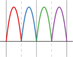
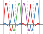
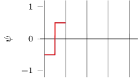
i.e, this is the classical orthogonal Haar basis, see Figures 7-8.

Figure 7: The primal and dual basis functions induced by $\mathcal{P}_{j}^{cg}$ at level $2$. For clarity, only one basis vector is shown in each element.

Figure 8: The primal and dual basis functions induced by $\mathcal{P}_{j}^{dg}$ at level $2$. For clarity, only one basis vector is shown in each element.

3.0.4 Piecewise polynomial predictors with stable projectors.

The local Gramm matrices $\mathbf{G}^{q}_{\scriptscriptstyle\Delta\Delta}$, $\mathbf{G}^{q}_{\scriptscriptstyle\Delta\nabla}$ of a varying order $q$ are defined in Appendix A.2. The update matrix spanning $r$ elements is then given by

$$\Big{(}\underbrace{\mathbf{G}^{q}_{\scriptscriptstyle\Delta\Delta}\oplus\ldots\oplus\mathbf{G}^{q}_{\scriptscriptstyle\Delta\Delta}}_{r\text{ times}}\Big{)}^{-1}\Big{(}\underbrace{\mathbf{G}^{q}_{\scriptscriptstyle\Delta\nabla}\ominus\ldots\ominus\mathbf{G}^{q}_{\scriptscriptstyle\Delta\nabla}}_{r\text{ times}}\Big{)}.$$

Therefore, the update matrix induced by the global projectors $\mathcal{P}_{j}^{cg}$ is given by

$$\mathbf{U}_{j}^{cg}=\Big{(}\underbrace{\mathbf{G}^{q}_{\scriptscriptstyle\Delta\Delta}\oplus\ldots\oplus\mathbf{G}^{q}_{\scriptscriptstyle\Delta\Delta}}_{2^{j}\text{ times}}\Big{)}^{-1}\Big{(}\underbrace{\mathbf{G}^{q}_{\scriptscriptstyle\Delta\nabla}\ominus\ldots\ominus\mathbf{G}^{q}_{\scriptscriptstyle\Delta\nabla}}_{2^{j}\text{ times}}\Big{)},$$ (45)

while the update matrix induced by the element-wise projectors $\mathcal{P}_{j}^{dg}$ is given by

$$\mathbf{U}_{j}^{dg}=\Big{(}\underbrace{\mathbf{I}_{\scriptscriptstyle{q+1}}\oplus\ldots\oplus\mathbf{I}_{\scriptscriptstyle{q+1}}}_{2^{j}\text{ times}}\Big{)}^{-1}\Big{(}\underbrace{\mathbf{U}^{q}\ominus\ldots\ominus\mathbf{U}^{q}}_{2^{j}\text{ times}}\Big{)}.$$ (46)

To clarify the meaning of the expression for $\mathbf{U}_{j}^{dg}$, consider the case with $q=1$ and $j=1$, which gives

$$\Big{(}\mathbf{I}_{\scriptscriptstyle{2}}\oplus\mathbf{I}_{\scriptscriptstyle{2}}\Big{)}^{-1}\Big{(}\mathbf{U}^{2}\ominus\mathbf{U}^{2}\Big{)} =\begin{bmatrix}1&&\\ &2&\\ &&1\end{bmatrix}^{-1}\begin{bmatrix}u_{00}&u_{01}&&\\ u_{10}&u_{11}&u_{00}&u_{01}\\ &&u_{10}&u_{11}\\ \end{bmatrix}$$

$$=\begin{bmatrix}u_{00}&u_{01}&&\\ \frac{u_{10}}{2}&\frac{u_{11}}{2}&\frac{u_{00}}{2}&\frac{u_{01}}{2}\\ &&u_{10}&u_{11}\\ \end{bmatrix}.$$

It is worth noting that the global update matrix $\mathbf{U}_{j}^{cg}$ is dense. Moreover, its evaluation requires inverting the banded matrix which adds to the computational complexity and scales with the problem size. On the other side, the matrix $\Big{(}\mathbf{U}^{q}\ominus\ldots\ominus\mathbf{U}^{q}\Big{)}$ in $\mathbf{U}_{j}^{dg}$ is comprised of identical blocks which can be explicitly precomputed. Figure 9 shows the costs of assembling and solving the linear systems required to evaluate the update matrices $\mathbf{U}^{cg}$ and $\mathbf{U}^{dg}$ in (45)-(46). Since evaluation of $\mathbf{U}^{dg}$ on the uniform grid requires matrix inversion just in one element, its cost is negligible and is omitted. At the same time, the cost of a banded linear solver in computing $\mathbf{U}^{cg}$ scales super-linearly with the problem size. The costs of assembling the matrices are also non-negligible and scale linearly. However, $\mathbf{U}^{cg}$ requires assembling two matrices while $\mathbf{U}^{dg}$ needs only one.

Figure 9: The costs of assembling and solving the linear systems in (45)-(46).

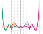
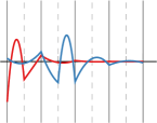
In either of two cases, the explicit representation of the basis functions is challenging. Figures 7-8 show the basis functions induced by $\mathcal{P}^{cg}$ and $\mathcal{P}^{dg}$ generated implicitly using the refinement equations in (28)-(29), (34)-(35). One can see that $\mathcal{P}^{cg}$ yield bases with global support while $\mathcal{P}^{dg}$ induced bases are supported only at the neighboring elements. Another observation is the fact that the dual basis functions are given by the superposition of $q$ different functions corresponding to different nodes of the elements. Particularly, the continuous functions in Figures 7-8 are obtained by connecting the values at the matching nodes of each element. Also note the the jump discontinuities at the boundaries of the interval.

3.1 Tensor grids

Extending the one-dimensional construction to the case of tensor grids is almost trivial. Given the matrix $\mathsf{M}$ of the one-dimensional transform in (24)-(25), one can simply use the Kronecker product as follows

$$\tilde{\boldsymbol{{\alpha}}}_{0} =\bigotimes_{d=1}^{D}\mathsf{M}\cdot\boldsymbol{{\alpha}}_{J},\qquad\boldsymbol{{\alpha}}_{J}=\bigotimes_{d=1}^{D}\mathsf{M}^{-1}\cdot\tilde{\boldsymbol{{\alpha}}}_{0}.$$

Alternatively, one can take the tensor product of the matrices in (23), and apply these transforms level-by-level. In wavelet methods, the first approach is referred to as fully separable transform, while the second approach, proposed by Mallat in [25], is more commonly employed in practice.

4 Results

4.1 Piecewise polynomials.

The proposed wavelet construction utilizes a hierarchical decomposition of piecewise polynomial spaces, which contrasts with the traditional translation-invariant filter bank formulation. In this example, we compare these two approaches by considering the function

$$f(x)=\sin(2\pi x)+\frac{1}{3}\sin(11\pi x)+\frac{1}{5}\sin(23\pi x),\qquad x\in[0,1],$$

and its piecewise linear interpolant $\mathcal{I}f$ defined on a grid with $N_{e}=2^{10}$ elements. The function $\mathcal{I}f$ is linear within each element and continuous across elements. Figure 3 illustrates this on a coarser grid.

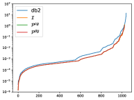
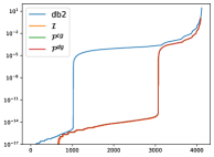
We evaluate this function at $N_{p}$ nodes of the uniform grid over the unit interval and compare the decay of the transform coefficients using Daubechies orthogonal wavelets (‘db2’) and three MGARD transforms with different projection operators. All considered transforms have two vanishing moments, meaning their wavelet bases are orthogonal to polynomials of orders zero and one. Additionally, MGARD wavelets are orthogonal to piecewise polynomials by design.

Figure 10 highlights these distinctions. It shows that while all transforms yield similar results when applied to data evaluated at the element nodes, the MGARD transform coefficients decay much faster when the data is sampled at multiple nodes within the elements. In contrast, Daubechies wavelets produce vanishing coefficients only when the wavelet is entirely contained within an element. The lack of $C^{1}$ smoothness across elements in the Daubechies wavelets results in larger coefficients that propagate through the hierarchy.

c0ptt-12pt$\mathcal{I}f(x)$   c0ptt-12pt$N_{e}=2^{10}$, $N_{p}=2^{10}$   c0ptt-12pt$N_{e}=2^{10}$, $N_{p}=2^{12}$

Figure 10: Sorted coefficients of the wavelet transforms with two vanishing moments for the piecewise linear function $\mathcal{I}f(x)$ defined on $N_{e}$ elements and evaluated at $N_{p}$ nodes.

4.2 Order comparison.

In this example, we study the impact of the order on data compression. As a measure of the compression quality, we use the $L^{2}$ error of the reconstructed signal as a function of the compression ratio (CR). Here we define the compression ratio as the relative number of the transform coefficients above the given threshold, and we do not consider quantization or entropy coding.

Figure 11 shows the coefficient decays and the compression ratios of the MGARD transform induced by global projectors $\mathcal{P}^{cg}$ of different orders. The top row depicts results for an image from the USC-SIPI image database. It can be observed that all methods perform nearly identically, with lower-order predictors performing the best. This is due to the limited smoothness of natural images, as explained in [12, 13]. Therefore, lower-order methods are expected to yield better results.

The second row of Figure 11 presents data from the boundary element (BEM) approximation of the solution to the Helmholtz equation describing scattering from a sphere. This data was generated using the boundary element software package in [6]. BEM solutions to the Laplace and Helmholtz equations are known to be smooth away from the boundary. This is evident from the decay of the wavelet coefficients for this problem. As a result, higher-order methods are much superior in this case, as indicated by the observed compression ratios.

c0ptt-12ptdata   c0ptt-12ptcoefficient decay   c0ptt-12ptcompression ratio vs error
c0ptt-12pt   c0ptt-12pt   c0ptt-12pt

Figure 11: Impact of the order on the compression ratio.

5 Conclusion and future work

In this work, we reformulated the MGARD algorithm as a wavelet transform on the interval. This reformulation provides new insights into the design and analysis of algorithm extensions. Specifically, we proposed a new family of projection operators that lead to compactly supported wavelet basis functions without compromising the stability of the transform. Moreover, the proposed formulation enables the construction of wavelets with an arbitrary number of vanishing moments by design. We demonstrated that this property results in better compression of data with matching regularity. Several questions remain to be addressed in future works, including data-adaptive order selection, optimal quantization, and rigorous error analysis.

Appendix A Appendix

A.1 Polynomial interpolation on dyadically nested uniform grids

Lemma A.1.

Given two nested one-dimensional uniform grids $\mathcal{G}_{0}\subset\mathcal{G}_{1}$ with $(r,2r)$ elements, $(rq,2rq)$ intervals, and $(rq+1,2rq+1)$ nodes respectively, the $q$-th order polynomial interpolation matrix $\mathbf{P}^{r,q}$ mapping the values $\{u_{2n}:n=0,\ldots,rq\}$ at the nodes of $\mathcal{G}_{0}$ to the values $\{u_{2m+1}:m=0,\ldots,rq-1\}$ at the nodes of the surplus grid $\mathcal{G}_{1}\setminus\mathcal{G}_{0}$ has the form

$$\mathbf{P}^{r,q}=\underbrace{\mathbf{P}^{q}\binrel@{\ominus}\binrel@@{\vphantom{\ominus}\mathchoice{\smash{\makebox[9.99997pt]{\rotatebox[origin={c}]{90.0}{$\displaystyle\ominus$}}}}{\smash{\makebox[9.99997pt]{\rotatebox[origin={c}]{90.0}{$\textstyle\ominus$}}}}{\smash{\makebox[7.66663pt]{\rotatebox[origin={c}]{90.0}{$\scriptstyle\ominus$}}}}{\smash{\makebox[6.11107pt]{\rotatebox[origin={c}]{90.0}{$\scriptscriptstyle\ominus$}}}}}\ldots\binrel@{\ominus}\binrel@@{\vphantom{\ominus}\mathchoice{\smash{\makebox[9.99997pt]{\rotatebox[origin={c}]{90.0}{$\displaystyle\ominus$}}}}{\smash{\makebox[9.99997pt]{\rotatebox[origin={c}]{90.0}{$\textstyle\ominus$}}}}{\smash{\makebox[7.66663pt]{\rotatebox[origin={c}]{90.0}{$\scriptstyle\ominus$}}}}{\smash{\makebox[6.11107pt]{\rotatebox[origin={c}]{90.0}{$\scriptscriptstyle\ominus$}}}}}\mathbf{P}^{q}}_{r\text{ times}},\qquad r>0,\;q\geq 0,$$

with $\binrel@{\ominus}\binrel@@{\vphantom{\ominus}\mathchoice{\smash{\makebox[9.99997pt]{\rotatebox[origin={c}]{90.0}{$\displaystyle\ominus$}}}}{\smash{\makebox[9.99997pt]{\rotatebox[origin={c}]{90.0}{$\textstyle\ominus$}}}}{\smash{\makebox[7.66663pt]{\rotatebox[origin={c}]{90.0}{$\scriptstyle\ominus$}}}}{\smash{\makebox[6.11107pt]{\rotatebox[origin={c}]{90.0}{$\scriptscriptstyle\ominus$}}}}}$ defined in Definition 2.2, $\mathbf{P}^{0}=[1]$, and

$$[\mathbf{P}^{q}]_{m,n}=\frac{(-1)^{m+n}}{2^{q}(1+2m-2n)}\frac{(2m+1)!!(2q-2m-1)!!}{n!(q-n)!},\qquad m =0,\ldots,q-1,$$

$$n =0,\ldots,q,\quad q>0,$$

where $p!!=1\cdot 3\cdot\ldots\cdot(p-2)p$ is the double factorial.

Proof.

The case of $q=0$ is trivial. For $q>0$, the values of the Lagrange interpolant $\mathcal{I}^{q}u$ at the nodes of $\mathcal{G}_{1}\setminus\mathcal{G}_{0}$ are given by

$$[\mathcal{I}^{q}u]_{2m+1} :=\sum_{n=0}^{q}u_{2n}\prod_{\begin{subarray}{c}k=0\\ k\neq n\end{subarray}}^{q}\frac{x_{2m+1}-x_{2k}}{x_{2n}-x_{2k}}$$

$$=\big{[}\mathbf{P}^{q}\cdot[u_{0},u_{2},\ldots,u_{2q}]^{T}\big{]}_{2m+1},\quad m=0,\ldots,q-1.$$

For a uniform grid with $x_{n}=nh$, we get

$$[\mathbf{P}^{q}]_{m,n} :=\prod_{\begin{subarray}{c}k=0\\ k\neq n\end{subarray}}^{q}\frac{x_{2m+1}-x_{2k}}{x_{2n}-x_{2k}}=\prod_{\begin{subarray}{c}k=0\\ k\neq n\end{subarray}}^{q}\frac{2(m-k)+1}{2(n-k)}.$$

To compute the denominator, collect the positive and negative terms in the product to get

$$\prod_{\begin{subarray}{c}k=0\\ k\neq n\end{subarray}}^{q}\frac{1}{2(n-k)}=\frac{1}{2^{q}}\prod_{k=0}^{n-1}\frac{1}{n-k}\prod_{k=n+1}^{q}\frac{1}{n-k}=\frac{1}{2^{q}}\frac{(-1)^{q-n}}{n!(q-n)!}.$$

Similarly, by collecting the positive and negative terms in the numerator, one gets

$$\prod_{\begin{subarray}{c}k=0\\ k\neq n\end{subarray}}^{q}(2(m-k)+1) =\frac{(-1)^{q-m}(2m+1)!!(2q-2m-1)!!}{1-2n+2m}.$$

∎

A.2 Gramm matrices for the elements of dyadically nested uniform grids.

Lemma A.2.

Under the same conditions as in Lemma A.1, the $q$-th order update matrix $\mathbf{U}^{r,q}$ mapping the values $\{u_{2m+1}:m=0,\ldots,rq-1\}$ at the nodes of the surplus grid $\mathcal{G}_{1}\setminus\mathcal{G}_{0}$ to the values $\{u_{2n}:n=0,\ldots,rq\}$ at the nodes of $\mathcal{G}_{0}$ has the form

$$\mathbf{U}^{r,q}:=\left(\mathbf{G}^{r,q}_{\scriptscriptstyle\Delta\Delta}\right)^{-1}\mathbf{G}^{r,q}_{\scriptscriptstyle\Delta\nabla}$$

where

$$\mathbf{G}^{r,q}_{\scriptscriptstyle\Delta\Delta} =\underbrace{\mathbf{G}^{q}_{\scriptscriptstyle\Delta\Delta}\oplus\ldots\oplus\mathbf{G}^{q}_{\scriptscriptstyle\Delta\Delta}}_{r\text{ times}},\qquad\mathbf{G}^{r,q}_{\scriptscriptstyle\Delta\nabla}=\underbrace{\mathbf{G}^{q}_{\scriptscriptstyle\Delta\nabla}\ominus\ldots\ominus\mathbf{G}^{q}_{\scriptscriptstyle\Delta\nabla}}_{r\text{ times}},\qquad r>0,\;q\geq 0$$

with $\oplus$ and $\ominus$ defined in Definition 2.2. The entries of the Gramm matrices are given by

$$\mathbf{G}_{\scriptscriptstyle\Delta\Delta}^{0}=[2h],\qquad\mathbf{G}_{\scriptscriptstyle\Delta\nabla}^{0}=[h]$$

and, for $q>0$,

$$[\mathbf{G}_{\scriptscriptstyle\Delta\Delta}^{q}]_{n,m}=\frac{2h(-1)^{n+m}}{n!m!(q-n)!(q-m)!}\int\displaylimits_{0}^{q}\frac{\prod_{\begin{subarray}{c}k=0\end{subarray}}^{q}(x-k)^{2}}{(x-n)(x-m)}dx,\qquad n=0,\ldots,q,\quad m=0,\ldots,q,$$

$$[\mathbf{G}_{\scriptscriptstyle\Delta\nabla}^{q}]_{n,m}=\frac{h(-1)^{n+1}}{2^{q}n!(q-n)!}$$

$$\times\begin{cases}\displaystyle\frac{1}{(2m+1)!(q-2m-1)!}\int\displaylimits_{0}^{q}\frac{\prod_{\begin{subarray}{c}k=0\end{subarray}}^{q}(x-2k)(x-k)}{(x-2n)(x-2m-1)}dx&m\leq q/2-1,\\[20.00003pt] \displaystyle\frac{1}{q!}\left[\int\displaylimits_{0}^{q}\frac{\prod_{\begin{subarray}{c}k=0\end{subarray}}^{q}(x-2k)(x-k)}{(x-2n)(x-2m-1)}dx-\int\displaylimits_{q}^{2q}\frac{\prod_{\begin{subarray}{c}k=0\end{subarray}}^{q}(x-2k)(x-k-q)}{(x-2n)(x-2m-1)}dx\right]&\displaystyle m=\frac{q-1}{2},\\[20.00003pt] \displaystyle\frac{(-1)^{q}}{(2m+1-q)!(2q-2m-1)!}\int\displaylimits_{q}^{2q}\frac{\prod_{\begin{subarray}{c}k=0\end{subarray}}^{q}(x-2k)(x-k-q)}{(x-2n)(x-2m-1)}dx&m\geq q/2\end{cases}$$

for $n=0,\ldots,q$, $m=0,\ldots,q-1$.

Proof.

The case of $q=0$ is trivial. For $q>0$, we get from the definition of Gram matrices

$$[\mathbf{G}_{\scriptscriptstyle\Delta\Delta}]_{n,m} :=\langle\varphi_{0,2n},\varphi_{0,2m}\rangle, \quad n=0,\ldots,q,\quad m=0,\ldots,q,$$

$$[\mathbf{G}_{\scriptscriptstyle\Delta\nabla}]_{n,m} :=\langle\varphi_{0,2n},\varphi_{1,2m+1}\rangle, \quad n=0,\ldots,q,\quad m=0,\ldots,q-1,$$

where $\varphi_{0}$, $\varphi_{1}$ are the Lagrange nodal basis functions on the grids $\mathcal{G}_{0}$, $\mathcal{G}_{1}$ respectively. For a uniform grid with $x_{n}=nh$, we get

$$\varphi_{0,2n}(x) =\prod_{\begin{subarray}{c}k=0\\ k\neq n\end{subarray}}^{q}\frac{x-2kh}{2(n-k)h},\qquad n=0,\ldots,q,\quad x\in[0,2hq],$$

and

$$\varphi_{1,2m+1} =\begin{cases}\displaystyle{\prod_{\begin{subarray}{c}k=0\\ k\neq 2m+1\end{subarray}}^{q}\frac{x-kh}{(2m+1-k)h}},&m=0,\ldots,\frac{q-1-(q-1)\%2}{2},\quad x\in[0,qh],\\[15.00002pt] \displaystyle{\prod_{\begin{subarray}{c}k=0\\ k+q\neq 2m+1\end{subarray}}^{q}\frac{x-(k+q)h}{(2m+1-q-k)h}},&m=\frac{q-1+(q-1)\%2}{2},\ldots,q-1,\quad x\in[qh,2qh],\end{cases}$$

where $(q-1)\%2\in\{0,1\}$ is the division remainder, i.e., $(q-1)\%2=0$ for odd $q$ and $(q-1)\%2=1$ otherwise. Hence, we have

$$[\mathbf{G}_{\scriptscriptstyle\Delta\Delta}]_{n,m} =\int_{0}^{2hq}\prod_{\begin{subarray}{c}k=0\\ k\neq n\end{subarray}}^{q}\frac{x-2kh}{2(n-k)h}\prod_{\begin{subarray}{c}k=0\\ k\neq m\end{subarray}}^{q}\frac{x-2kh}{2(m-k)h}dx=2h\int_{0}^{q}\prod_{\begin{subarray}{c}k=0\\ k\neq n\end{subarray}}^{q}\frac{x-k}{n-k}\prod_{\begin{subarray}{c}k=0\\ k\neq m\end{subarray}}^{q}\frac{x-k}{m-k}dx$$

$$=2h\frac{(-1)^{n+m}}{n!m!(q-n)!(q-m)!}\int_{0}^{q}\frac{\prod_{\begin{subarray}{c}k=0\end{subarray}}^{q}(x-k)^{2}}{(x-n)(x-m)}dx.$$

Similarly, for $m\leq q/2-1$, we have

$$[\mathbf{G}_{\scriptscriptstyle\Delta\nabla}]_{n,m} :=\int_{0}^{qh}\prod_{\begin{subarray}{c}k=0\\ k\neq n\end{subarray}}^{q}\frac{x-2kh}{2(n-k)h}\prod_{\begin{subarray}{c}k=0\\ k\neq 2m+1\end{subarray}}^{q}\frac{x-kh}{(2m+1-k)h}dx$$

$$=\frac{h}{2^{q}}\int_{0}^{q}\prod_{\begin{subarray}{c}k=0\\ k\neq n\end{subarray}}^{q}\frac{x-2k}{n-k}\prod_{\begin{subarray}{c}k=0\\ k\neq 2m+1\end{subarray}}^{q}\frac{x-k}{2m+1-k}dx$$

$$=\frac{h}{2^{q}}\frac{(-1)^{n+1}}{n!(2m+1)!(q-n)!(q-2m-1)!}\int_{0}^{q}\frac{\prod_{\begin{subarray}{c}k=0\end{subarray}}^{q}(x-2k)(x-k)}{(x-2n)(x-2m-1)}dx$$

and for $m\geq q/2$, we get

$$[\mathbf{G}_{\scriptscriptstyle\Delta\nabla}]_{n,m} :=\int_{qh}^{2qh}\prod_{\begin{subarray}{c}k=0\\ k\neq n\end{subarray}}^{q}\frac{x-2kh}{2(n-k)h}\prod_{\begin{subarray}{c}k=0\\ k+q\neq 2m+1\end{subarray}}^{q}\frac{x-(k+q)h}{(2m+1-q-k)h}dx$$

$$=\frac{h}{2^{q}}\int_{q}^{2q}\prod_{\begin{subarray}{c}k=0\\ k\neq n\end{subarray}}^{q}\frac{x-2k}{n-k}\prod_{\begin{subarray}{c}k=0\\ k+q\neq 2m+1\end{subarray}}^{q}\frac{x-(k+q)}{2m+1-q-k}dx$$

$$=\frac{h}{2^{q}}\frac{(-1)^{n+q+1}}{n!(2m+1-q)!(q-n)!(2q-2m-1)!}\int_{q}^{2q}\frac{\prod_{\begin{subarray}{c}k=0\end{subarray}}^{q}(x-2k)(x-k-q)}{(x-2n)(x-2m-1)}dx.$$

For $q$ odd and $m=\frac{q-1}{2}$, we also have

$$[\mathbf{G}_{\scriptscriptstyle\Delta\nabla}]_{n,m} :=\frac{h}{2^{q}}\int_{0}^{q}\prod_{\begin{subarray}{c}k=0\\ k\neq n\end{subarray}}^{q}\frac{x-2k}{n-k}\prod_{\begin{subarray}{c}k=0\\ k\neq 2m+1\end{subarray}}^{q}\frac{x-k}{2m+1-k}dx$$

$$+\frac{h}{2^{q}}\int_{q}^{2q}\prod_{\begin{subarray}{c}k=0\\ k\neq n\end{subarray}}^{q}\frac{x-2k}{n-k}\prod_{\begin{subarray}{c}k=0\\ k+q\neq 2m+1\end{subarray}}^{q}\frac{x-(k+q)}{2m+1-q-k}dx$$

$$=\frac{h}{2^{q}}\frac{(-1)^{n+1}}{n!(q-n)!(2m+1)!(q-2m-1)!}\left[\int_{0}^{q}\frac{\prod_{\begin{subarray}{c}k=0\end{subarray}}^{q}(x-2k)(x-k)}{(x-2n)(x-2m-1)}dx\right.$$

$$+(-1)^{q}\left.\frac{(2m+1)!(q-2m-1)!}{(2m+1-q)!(2q-2m-1)!}\int_{q}^{2q}\frac{\prod_{\begin{subarray}{c}k=0\end{subarray}}^{q}(x-2k)(x-k-q)}{(x-2n)(x-2m-1)}dx\right]$$

$$=\frac{h}{2^{q}}\frac{(-1)^{n+1}}{n!q!(q-n)!}\left[\int_{0}^{q}\frac{\prod_{\begin{subarray}{c}k=0\end{subarray}}^{q}(x-2k)(x-k)}{(x-2n)(x-q)}dx-\int_{q}^{2q}\frac{\prod_{\begin{subarray}{c}k=0\end{subarray}}^{q}(x-2k)(x-k-q)}{(x-2n)(x-q)}dx\right].$$

∎

References

• [1] Milton Abramowitz, Irene A Stegun, and Robert H Romer. Handbook of mathematical functions with formulas, graphs, and mathematical tables. American Association of Physics Teachers, 1988.
• [2] Mark Ainsworth, Ozan Tugluk, Ben Whitney, and Scott Klasky. Multilevel techniques for compression and reduction of scientific data – the univariate case. Computing and Visualization in Science, 19:65–76, 2018.
• [3] Mark Ainsworth, Ozan Tugluk, Ben Whitney, and Scott Klasky. Multilevel techniques for compression and reduction of scientific data – the multivariate case. SIAM Journal on Scientific Computing, 41:A1278–A1303, 1 2019.
• [4] Mark Ainsworth, Ozan Tugluk, Ben Whitney, and Scott Klasky. Multilevel techniques for compression and reduction of scientific data-quantitative control of accuracy in derived quantities. SIAM Journal on Scientific Computing, 41:A2146–A2171, 1 2019.
• [5] Mark Ainsworth, Ozan Tugluk, Ben Whitney, and Scott Klasky. Multilevel techniques for compression and reduction of scientific data – the unstructured case. SIAM Journal on Scientific Computing, 42:A1402–A1427, 2020.
• [6] Timo Betcke and Matthew Scroggs. Bempp-cl: A fast python based just-in-time compiling boundary element library. Journal of Open Source Software, 6(59):2879–2879, 2021.
• [7] Folkmar Bornemann and Harry Yserentant. A basic norm equivalence for the theory of multilevel methods. Numerische Mathematik, 64:455–476, 12 1993.
• [8] Peter J. Burt and Edward H. Adelson. The Laplacian pyramid as a compact image code. In Martin A. Fischler and Oscar Firschein, editors, Readings in Computer Vision, pages 671–679. Morgan Kaufmann, San Francisco (CA), 1987.
• [9] Albert Cohen. Numerical analysis of wavelet methods. Elsevier, New York, 2003.
• [10] Wolfgang Dahmen. Stability of multiscale transformations. The journal of Fourier analysis and applications [[Elektronische Ressource]], 2:341–362, 1995.
• [11] Ingrid Daubechies and Wim Sweldens. Factoring wavelet transforms into lifting steps. Journal of Fourier analysis and applications, 4:247–269, 1998.
• [12] R.A. DeVore, B. Jawerth, and B.J. Lucier. Image compression through wavelet transform coding. IEEE Transactions on Information Theory, 38(2):719–746, 1992.
• [13] R.A. DeVore and B.J. Lucier. Classifying the smoothness of images: theory and applications to wavelet image processing. In Proceedings of 1st International Conference on Image Processing, volume 2, pages 6–10 vol.2, 1994.
• [14] Minh N. Do and Yue M. Lu. Multidimensional filter banks and multiscale geometric representations. Foundations and Trends in Signal Processing, 5(3):157–264, 2012.
• [15] Norbert J Fliege. Multirate digital signal processing: multirate systems, filter banks, wavelets. John Wiley & Sons, Inc., 1994.
• [16] Michael S. Floater, Géza Kós, and Martin Reimers. Mean value coordinates in 3d. Computer Aided Geometric Design, 22(7):623–631, 2005. Geometric Modelling and Differential Geometry.
• [17] Qian Gong, Jieyang Chen, Ben Whitney, Xin Liang, Viktor Reshniak, Tania Banerjee, Jaemoon Lee, Anand Rangarajan, Lipeng Wan, Nicolas Vidal, Qing Liu, Ana Gainaru, Norbert Podhorszki, Richard Archibald, Sanjay Ranka, and Scott Klasky. MGARD: A multigrid framework for high-performance, error-controlled data compression and refactoring. SoftwareX, 24, 12 2023.
• [18] Qian Gong, Jieyang Chen, Ben Whitney, Xin Liang, Viktor Reshniak, Tania Banerjee, Jaemoon Lee, Anand Rangarajan, Lipeng Wan, Nicolas Vidal, Qing Liu, Ana Gainaru, Norbert Podhorszki, Richard Archibald, Sanjay Ranka, and Scott Klasky. MGARD: A multigrid framework for high-performance, error-controlled data compression and refactoring. SoftwareX, 24:101590, 2023.
• [19] Qian Gong, Chengzhu Zhang, Xin Liang, Viktor Reshniak, Jieyang Chen, Anand Rangarajan, Sanjay Ranka, Nicolas Vidal, Lipeng Wan, Paul Ullrich, Norbert Podhorszki, Robert Jacob, and Scott Klasky. Spatiotemporally adaptive compression for scientific dataset with feature preservation – a case study on simulation data with extreme climate events analysis. In 2023 IEEE 19th International Conference on e-Science (e-Science), pages 1–10, 2023.
• [20] Michael W. Hackemack and Jean C. Ragusa. Quadratic serendipity discontinuous finite element discretization for sn transport on arbitrary polygonal grids. Journal of Computational Physics, 374:188–212, 2018.
• [21] Dmitry Kolomenskiy, Ryo Onishi, and Hitoshi Uehara. WaveRange: wavelet-based data compression for three-dimensional numerical simulations on regular grids. Journal of Visualization, 25(3):543–573, 2022.
• [22] Sriram Lakshminarasimhan, Neil Shah, Stephane Ethier, Seung-Hoe Ku, Choong-Seock Chang, Scott Klasky, Rob Latham, Rob Ross, and Nagiza F Samatova. ISABELA for effective in situ compression of scientific data. Concurrency and Computation: Practice and Experience, 25(4):524–540, 2013.
• [23] Jaemoon Lee, Qian Gong, Jong Choi, Tania Banerjee, Scott Klasky, Sanjay Ranka, and Anand Rangarajan. Error-bounded learned scientific data compression with preservation of derived quantities. Applied Sciences, 12(13), 2022.
• [24] Shaomeng Li, Peter Lindstrom, and John Clyne. Lossy scientific data compression with SPERR. In 2023 IEEE International Parallel and Distributed Processing Symposium (IPDPS), pages 1007–1017, 2023.
• [25] S.G. Mallat. A theory for multiresolution signal decomposition: the wavelet representation. IEEE Transactions on Pattern Analysis and Machine Intelligence, 11(7):674–693, 1989.
• [26] Peter Oswald. Multilevel Finite Element Approximation. Vieweg+Teubner Verlag Wiesbaden, 1994.
• [27] W.A. Pearlman, A. Islam, N. Nagaraj, and A. Said. Efficient, low-complexity image coding with a set-partitioning embedded block coder. IEEE Transactions on Circuits and Systems for Video Technology, 14(11):1219–1235, 2004.
• [28] Jean-Luc Peyrot, Laurent Duval, Frédéric Payan, Lauriane Bouard, Lénaïc Chizat, Sébastien Schneider, and Marc Antonini. HexaShrink, an exact scalable framework for hexahedral meshes with attributes and discontinuities: multiresolution rendering and storage of geoscience models. Computational Geosciences, 23(4):723–743, May 2019.
• [29] P. Roos, M.A. Viergever, M.C.A. van Dijke, and J.H. Peters. Reversible intraframe compression of medical images. IEEE Transactions on Medical Imaging, 7(4):328–336, 1988.
• [30] Khalid Sayood. Introduction to Data Compression. The Morgan Kaufmann Series in Multimedia Information and Systems. Morgan Kaufmann, 2006.
• [31] Emre Sermutlu. A close look at Newton–Cotes integration rules. Results in Nonlinear Analysis, 2(2):48–60, Nov. 2022.
• [32] Mallat Stéphane. A Wavelet Tour of Signal Processing. Academic Press, 2009.
• [33] Wim Sweldens and Peter Schröder. Building your own wavelets at home. In Roland Klees and Roger Haagmans, editors, Wavelets in the Geosciences, pages 72–107. Springer, Berlin, Heidelberg, 2005.
• [34] David S. Taubman and Michael W. Marcellin. JPEG2000 Image Compression Fundamentals, Standards and Practice. The Springer International Series in Engineering and Computer Science. Springer New York, NY, 2002.
• [35] P.P. Vaidyanathan. Multirate digital filters, filter banks, polyphase networks, and applications: a tutorial. Proceedings of the IEEE, 78(1):56–93, 1990.
• [36] M.A. Viergever and P. Roos. Hierarchical interpolation. IEEE Engineering in Medicine and Biology Magazine, 12(1):48–55, 1993.
• [37] Jinchao Xu. Iterative methods by space decomposition and subspace correction. SIAM Review, 34:581–613, 1992.
• [38] Kai Zhao, Sheng Di, Xin Lian, Sihuan Li, Dingwen Tao, Julie Bessac, Zizhong Chen, and Franck Cappello. Sdrbench: Scientific data reduction benchmark for lossy compressors. In 2020 IEEE International Conference on Big Data (Big Data), pages 2716–2724, 2020.