Maximizing $\mathcal{V}$-information for Pre-training Superior Foundation Models

Abstract

Pre-training foundation models on large-scale datasets demonstrates exceptional performance. However, recent research questions this traditional notion, exploring whether an increase in pre-training data always leads to enhanced model performance. To address this issue, data-effective learning approaches have been introduced. However, current methods in this area lack a clear standard for sample selection. Our experiments reveal that by maximizing $\mathcal{V}$-information, sample selection can be framed as an optimization problem, enabling effective improvement in model performance even with fewer samples. Under this guidance, we develop an optimal data-effective learning method (OptiDEL) to maximize $\mathcal{V}$-information. The OptiDEL method generates hard samples to achieve or even exceed the performance of models trained on the full dataset while using substantially less data. We compare the OptiDEL method with state-of-the-art approaches finding that OptiDEL consistently outperforms existing approaches across different datasets, with foundation models trained on only 5% of the pre-training data surpassing the performance of those trained on the full dataset. The code can be accessed at GitHub Repository.

Introduction

Pre-training foundation models on large-scale datasets has become a standard practice, as it significantly boosts model performance and generalization capabilities (Kolides et al. 2023). However, recent research (Yang et al. 2024) has questioned this conventional wisdom: does more pre-training data invariably lead to improved model performance? To investigate this, (Yang et al. 2024) introduced a benchmark for data-effective learning, exploring the significant nonlinear phenomenon exhibited by foundation models trained with different proportions of data on a given dataset. However, this phenomenon has so far lacked a theoretical explanation.

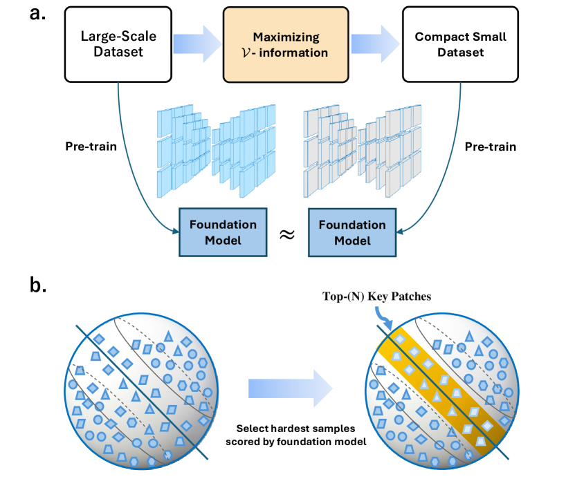
Figure 1: (a) By maximizing $\mathcal{V}$-information, we can generate a smaller unlabeled dataset from a larger unlabeled dataset, with minimal differences in the pre-training results of foundation models. (b) $\mathcal{V}$-information theory shows that selecting the hardest-N samples enables a smaller selection ratio without sacrificing model performance.

Fortunately, in the field of supervised learning, numerous mature methods have been developed to enhance both data utilization efficiency and model performance  (Bai et al. 2024). These methods are primarily divided into two categories: coreset-based and optimization-based approaches (Ceccarello, Pietracaprina, and Pucci 2018). Optimization-based methods employ complex optimization strategies to enhance the representational power of datasets while reducing the volume of data required for training. These techniques have achieved notable strides in lowering computational costs and enhancing model performance. On the other hand, coreset-based methods concentrate on selecting a subset of samples from the original dataset that accurately represents the entire dataset. They are recognized for their computational efficiency and their capacity to preserve the representativeness of the original dataset. However, migrating these techniques from supervised to unsupervised learning remains a major challenge, particularly in terms of computational complexity and theoretical validation.

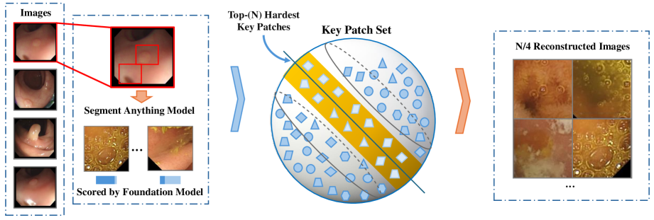
Figure 2: Visualization of our OptiDEL method framework. First, SAM is used to extract patches with potential lesions from the original image. These patches are then evaluated based on their reconstruction errors to identify the hardest key examples. Next, every $M$ of these key patches is combined to create a new image, maintaining the original image’s resolution.

Inspired by $\mathcal{V}$-information theory, we frame data-effective learning task as an optimization problem of conditional entropy Fig 1(a). It particularly emphasizes that selecting hard samples can potentially match or even surpass the performance of models trained on the full dataset while utilizing fewer data Fig 1(b). Guided by this theory, we develop the optimal data-effective learning (OptiDEL) method, which generates harder pre-training samples from the original data and extracts critical information through the segment anything model (SAM). The key concept behind this method is to create pre-training samples with greater difficulty and more diverse information, aiming to approximate the optimal performance of a foundation model under ideal conditions.

The key contributions of this paper can be summarized as:

• This paper transforms the task of sample selection in data-effective learning into an optimization problem of maximizing $\mathcal{V}$-information which emphasizes that the key to an ideal data-effective learning approach lies in extracting information from challenging samples. This insight guides the development of more effective methods, aiming to enhance performance through strategic sample selection.

• Based on the $\mathcal{V}$-information theory, we design the OptiDEL method which enhances the performance of foundation models by generating hard samples through the extraction of critical data information using the SAM model.

• We compare our OptiDEL with the state-of-the-art MedDEL (Yang et al. 2024) across eight real medical datasets. Our experimental results highlight the importance of maximizing $\mathcal{V}$-information for improving data-effective learning performance.

Related Work

Data distillation (Lei and Tao 2023) is a technique aimed at reducing large-scale datasets by synthesizing or selectively extracting key samples to improve learning efficiency and reduce computational resource demands.

Traditional data distillation. In the field of supervised learning, traditional data distillation can be mainly divided into two categories: optimization-based methods and coreset-based methods.

Optimization-based methods are a crucial direction of exploration, which enhance dataset representation while reducing the amount of data required through a series of complex optimization strategies. These strategies encompass various techniques such as bi-level optimization  (Wang et al. 2018) and uni-level optimization  (Nguyen et al. 2021; Loo et al. 2023). Bi-level optimization methods aim to minimize the discrepancy between surrogate models learned from synthetic data and original data. These methods typically involve two optimization processes: outer optimization adjusts the high-level parameters of the model, while inner optimization adjusts the low-level parameters to ensure the model’s performance remains as consistent as possible across different datasets. Specifically, these methods rely on metrics such as gradient matching (Zhao, Mopuri, and Bilen 2021; Killamsetty et al. 2021), feature matching (Ji, Heo, and Park 2021), distribution matching (Zhang et al. 2021; Binici et al. 2022), and training trajectory (Cazenavette et al. 2022; Guo et al. 2023) matching to ensure consistency in model performance across different datasets. The advantage of bi-level optimization methods lies in their ability to handle complex data distributions and tasks. However, due to their high computational complexity and resource consumption, they may face performance bottlenecks and efficiency issues in practical applications. Uni-level optimization methods, on the other hand, simplify the optimization process to reduce training costs and improve performance, thus achieving efficient data distillation. For instance, kernel ridge regression methods (Nguyen, Chen, and Lee 2021; Xu et al. 2023) adopt uni-level optimization strategies by solving a regularized linear regression problem to reduce the computational burden. This approach significantly reduces the consumption of computational resources while demonstrating excellent performance in handling large-scale datasets. The key to uni-level optimization methods lies in reducing the complexity of optimization and simplifying the model training process, making data distillation more efficient. Although uni-level optimization methods exhibit better efficiency in handling large-scale datasets, they may not fully capture the complexity of data and the characteristics of tasks in certain complex scenarios.

In contrast, coreset-based methods (Mirzasoleiman, Bilmes, and Leskovec 2020; Pooladzandi, Davini, and Mirzasoleiman 2022) focus on identifying and selecting a subset of samples that can represent the entire dataset. These methods are gaining attention for their computational efficiency and ability to retain the representativeness of the original dataset. They typically utilize metrics such as Forgetting Score (Toneva et al. 2019), Memorization (Feldman and Zhang 2020), and EL2N Score (Paul, Ganguli, and Dziugaite 2021) to evaluate the importance of samples. Additionally, they employ Diverse Ensembles strategies to ensure that the selected samples comprehensively cover the diversity present in the dataset.

Data-effective learning methods. Unlike traditional supervised data distillation, (Yang et al. 2024) have proposed a comprehensive benchmark specifically designed to evaluate data-effective learning in the medical field. This research focuses on unsupervised data-effective learning aimed at efficiently training foundation models. The benchmark includes a dataset with millions of data samples from 31 medical centers (DataDEL), a baseline method for comparison (MedDEL), and a new evaluation metric (NormDEL) to objectively measure the performance of data-effective learning. This benchmark lays the foundation for the pre-training and theoretical validation of foundation models.

Methodology

(Yang et al. 2024) have provided a benchmark in the field of medical date-effective learning. However, their approach is relatively fundamental, leaving substantial room for further exploration. In the following sections, we demonstrate that the DEL task can be framed as an optimization problem by maximizing $\mathcal{V}$-information. Building on this foundation and incorporating principles from information theory, we will also detail our OptiDEL algorithm.

Preliminary

Data-effective learning. The goal of data-effective learning is to generate a small-scale dataset $S=\left\{X|X=x_{i}\right\}_{i=1}^{|S|}$ from a large number of unlabeled data samples $D=\left\{\hat{X}|\hat{X}=\hat{x}_{j}\right\}_{j=1}^{|D|}$, where $|S|\ll|D|$. The essence of this approach is to ensure that the pre-training performance of the foundation model on the small dataset $S$ is comparable to its performance on the large dataset $D$ within an acceptable error range. This goal can be expressed by the following equation:

$$\mathop{\mathrm{sup}}\limits_{x\sim D}\left\{|l(\phi_{D}(x),x)-l(\phi_{S}(x),x)|\right\}\leq\epsilon.$$ (1)

We utilize a Masked Auto Encoder (MAE) (He et al. 2022) for unsupervised training, a process based on Vision Transformers (ViT) (Dosovitskiy et al. 2020) to generate the original image $x$. In the above equation, $\phi(\cdot)$ represents the MAE model, $l$ denotes the mean squared error loss, and $\theta_{D}=\mathrm{arg\,min}_{\theta}\mathbf{E}_{(x,y)\in D}\,l(\phi_{\theta}(x),x)$.

Maximize the $\mathcal{V}$-information of the original image.  (Sun et al. 2024) proposed a supervised data distillation method based on $\mathcal{V}$-information theory (Xu et al. 2020). Specifically, from the perspective of $\mathcal{V}$-information, we aim to select a smaller subset $S$ from the dataset $D$ that maximizes the information from the input variable $X$ to the output variable $Y$ i.e., maximizing the conditional entropy of $X$ given $Y$. Therefore, Equation 1 can be rewritten as:

$$S=\mathop{arg\max}\limits_{x\in A\left(T\right)}I_{\mathcal{V}}\left(X\rightarrow Y\right),$$ (2)

where $I_{\mathcal{V}}=\mathop{inf}\limits_{f\in\mathcal{V}}\sum{\frac{1}{|D|}\log\frac{1}{f\left[\oslash\right]\left(Y\right)}-}\mathop{inf}\limits_{f\in\mathcal{V}}\sum{\frac{1}{|D|}\log\frac{1}{f\left[X\right]\left(Y\right)}}.$ In the unsupervised MAE task, the input $X$ corresponds to the original image, and the output $Y$ corresponds to the model’s reconstructed image. In this equation, $f\left[\oslash\right]\left(Y\right)$ represents the probability density function of the output $Y$ given no additional information, while $f\left[X\right]\left(Y\right)$ represents the probability density function of the output $Y$ given the information $X$.

Our optimization goal is to maximize the conditional $\mathcal{V}$-information of $X$ given $Y$, which requires maximizing the first term and minimizing the second term. Maximizing the first term implies that the marginal distribution of $Y$ has a high level of uncertainty, meaning that $Y$’s state has a wide range of variations, thereby enhancing the diversity of the samples. Minimizing the second term indicates that given $X$, we can reduce the uncertainty of $Y$ as much as possible, meaning that $X$ provides sufficient information to predict $Y$ accurately, thus enhancing the accuracy of the samples.

Selecting hard samples helps to further enhance the $\mathcal{V}$-information. Recent studies (Toneva et al. 2019; Feldman and Zhang 2020; Paul, Ganguli, and Dziugaite 2021) have investigated different metrics for assessing the variability between training examples. In this context, (Sorscher et al. 2022) discusses these metrics as methods for ranking samples based on their difficulty. For example, samples with the highest average $L_{2}$ norm of the error vector, known as the EL2N score, are considered hard examples.

To provide context, the model $\phi_{D}$ trained on the full dataset $D$ actually has a deviation $\theta$ from the ideal foundation model $\phi_{I}$, which perfectly reconstructs every example. $\phi_{S}$ is the model trained on the selected subset $S$. Our primary concern is the fitting error $e$ between $\phi_{S}$ and $\phi_{I}$.

Building on (Sorscher et al. 2022)’s data pruning theory, our research delves deeper into the relationship between $e$ and the data selection ratio $f$, maintaining a constant total data volume. Our main result is that by selecting the hardest samples from the dataset $D$, a smaller selection ratio $f$ can be employed without sacrificing model performance as the original data volume increases.

The main result of our study underscores the crucial property of maximizing the $\mathcal{V}$-information. By specifically targeting and learning from the hardest samples, the model is able to significantly reduce its overall uncertainty. This approach not only enhances the model’s ability to generalize across unseen data but also ensures that it is robust against variations within the data, thereby stabilizing its predictions in more challenging or diverse scenarios. We also analyze whether this property can be maintained under different $\theta$ values, with data redundancy and downstream task bias factors. The theoretical explanations are in the appendix, with numerical results and analysis in the experimental section.

Algorithm 1 Pseudo Code for OptiDEL

Input: Dataset $D$ and a pre-trained foundation model $\phi_{D}$
Parameter: $N,K,M$

1:  for $\hat{x_{i}}\in D$  do

2:     Utilize SAM to crop $\hat{x_{i}}$ into $N$ patches $\{\xi_{i}\}_{i=1}^{N}$.

3:  end for

4:  get patches set $\{\xi_{i}\}_{i=1}^{N\times|D|}$.

5:  for $i=1\,\text{to}\,N\times|D|$ do

6:     Calculate margin $m_{i}=l\left(\phi_{D}(\xi_{i}),\xi_{i}\right)$ of patch $\xi_{i}$.

7:  end for

8:  Select top-$K$ margin patches $\{\xi^{{}^{\prime}}_{i}\}_{i=1}^{K}$

9:  for $i=1\,\text{to}\,K$ do

10:     if $(i\,\text{mod}\,M\text{==}0)$ then

11:        Synthesize $M$ patches $\{\xi^{{}^{\prime}}_{j}\}_{j=i+1-M}^{i}$ into a new image $X_{j}$

12:     end if

13:  end for

Output: Synthesized dataset $S=\{X|X=X_{j}\}$ and the final foundation model $\phi_{S}$ trained from scratch on $S$

Details of OptiDEL Algorithm

In this section, we provide the details of the proposed OptiDEL algorithm. A simplified version of the OptiDEL algorithm is illustrated through the pseudocode presented in Algorithm 1.

Using SAM to extract key information. Based on $\mathcal{V}$-information theory (Xu et al. 2020), we extract several patches from the original image and use them for subsequent pre-training of the foundation model to improve the authenticity of the data. Current methods (Sun et al. 2024) involve random patch cropping, followed by selecting the top-$k$ patches based on the foundation model’s scores, which inherently introduces a degree of randomness. Ideally, we propose leveraging the segment anything model (SAM) (Kirillov et al. 2023) to extract potential lesions in medical images proactively. The entire process can be formulated as:

$$\xi_{i,*}=S\left(\hat{x}_{i}\right)=\left\{S\left(\hat{x}_{i,1}\right),\cdots,S\left(\hat{x}_{i,k}\right)\right\}.$$ (3)

Subsequently, we apply this operation to all the original images, resulting in $S=\{\xi_{i,*}\}_{i=1}^{|D|}=\{\xi_{i}\}_{i=1}^{N\times|D|}$, where $\xi_{i,k}$ represents the $k^{th}$ patch extracted from the $i^{th}$ image.

Select patches as hard examples. The MAE model can be considered a function that maps a masked input back to its original version, which can perfectly reconstruct patches in the ideal situation, with the ideal model denoted as $\phi_{I}$. However, in practice, some patches are difficult to reconstruct while others are relatively easier, leading to variable reconstruction errors in actual trained foundation model $\phi_{D}$. Inspired by this, we define the margin $m_{i}$ for the patch $\xi_{i}$ based on the reconstruction loss from model $\phi_{D}$:

$$m_{i}=l\left(\phi_{D}(\xi_{i}),\xi_{i}\right).$$ (4)

(a) $\theta$ between $\phi_{I}$ and $\phi_{D}$.

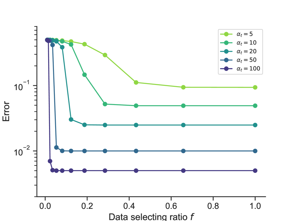
(b) $\theta=0^{\circ}$.

(c) $\theta=10^{\circ}$.

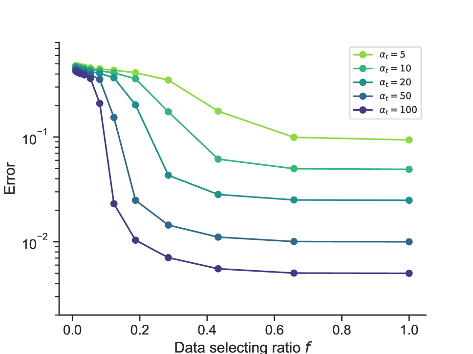
(d) $\theta=20^{\circ}$.

Figure 3: The correlation between the parameter $f$ (selection ratio) and the fitting error (involving the ideal optimal model $\phi_{I}$ and the model trained with distilled data $\phi_{S}$) across different total data sizes $\alpha_{t}$ and angles $\theta$ (involving $\phi_{I}$ and the pre-trained model trained with 100% data $\phi_{D}$). Moreover, as the angle $\theta$ increases, the model’s fitting error increases as well. However, even with a larger amount of original data, we can still choose a smaller ratio $f$ for the pretraining data.

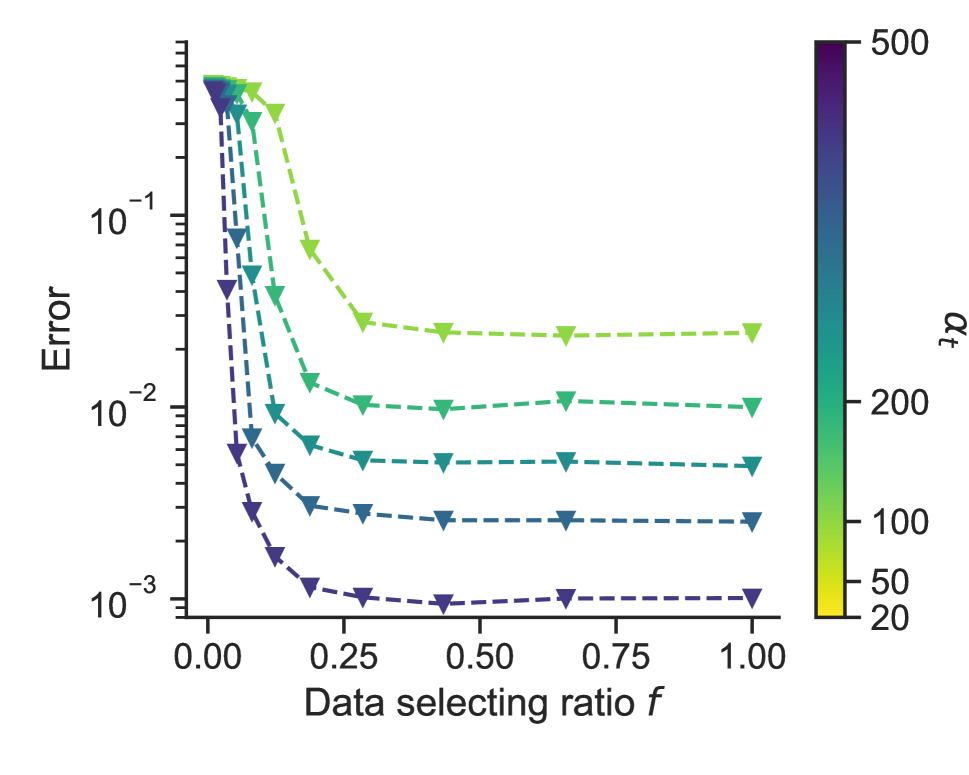
(a) No data redundancy.

(b) 3x data redundancy.

(c) 5x data redundancy.

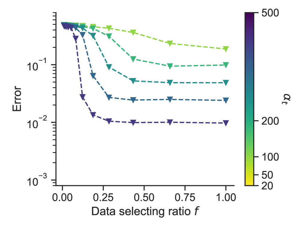
(d) 10x data redundancy.

Figure 4: The correlation between the fitting error (involving the ideal optimal model $\phi_{I}$ and the model trained with distilled data $\phi_{S}$) and the data selection ratio $f$ across different levels of data redundancy (0x, 3x, 5x, 10x), here we set $\theta=10^{\circ}$. The results demonstrate that as data redundancy increases, selecting a small proportion of the dataset still yields performance comparable to using the full dataset. This indicates the potential in real-world training scenarios to distill more effective datasets from larger data pools with redundant data.

(a) Downstream tasks.

(b) Downstream task bias $\epsilon=0.1$

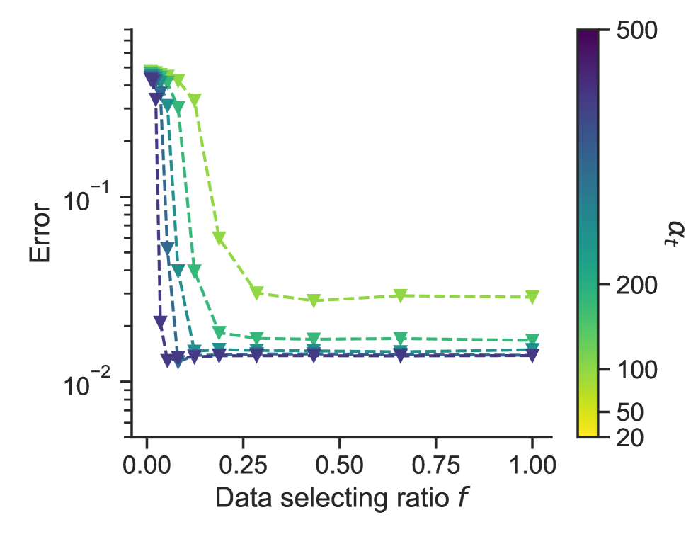
(c) Downstream task bias $\epsilon=0.2$

(d) Downstream task bias $\epsilon=0.3$

Figure 5: The correlation between the parameter $f$ and the fitting error (involving the ideal optimal model for downstream tasks $\phi_{I^{\prime}}$ and the model trained with distilled data $\phi_{S}$) across different total data volumes $\alpha_{t}$ and downstream task biases $\epsilon$, here we set $\theta=10^{\circ}$. As $\epsilon$ increases, the performance of the pre-trained model significantly declines, indicating that when the discrepancy between upstream and downstream tasks is large, the performance of the selected model also deteriorates. Despite this, the overall trend remains stable, suggesting that even with a very small data selection ratio $f$, it is possible to achieve the performance of models trained on the full dataset.

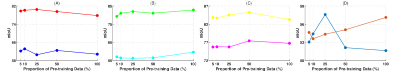
(a) DPT’s performance of MedDEL method on A: Kvasir-Instrument (red ) and Kvasir-SEG (blue ). B: CVC-ClinicDB (green ) and ImageCLEFmed (cyan ). C: CVC-ColonDB (magenta ) and CVC-300 (yellow ). D: ETIS (prussian blue ) and PolypGen2021 (dark orange ).

(b) DPT’s performance of OptiDEL method on E: Kvasir-Instrument (red ) and Kvasir-SEG (blue ). F: CVC-ClinicDB (green ) and ImageCLEFmed (cyan ). G: CVC-ColonDB (magenta ) and CVC-300 (yellow ). H: ETIS (prussianblue ) and PolypGen2021 (dark orange ).

Figure 6: On eight different downstream datasets, we employ DPT as the segmentation network, using both MedDEL and OptiDEL algorithms to assess the impact of different pre-training data ratios on foundation model performance. Our experimental results consistently show that in most cases, model performance typically follows a pattern of initial improvement followed by a decline. This trend closely resembles the expected performance changes under ideal experimental conditions, indicating that after reaching a certain level of training data, further increases do not enhance performance and may even lead to decreases due to factors such as overfitting. Specifically, we find that using the MedDEL algorithm with pre-training data ratios of 25% and 50% generally yields better performance than higher ratios, while for OptiDEL, the optimal ratios are 10% and 25%.

We classify patches with higher margins as harder training examples, while those with smaller margins are considered easier. According to the property of maximizing $\mathcal{V}$-information, prioritizing patches with the largest margins for subsequent synthesis not only saves computation time but also maintains or even enhances the model’s performance.

Patches synthesis. After selecting image patches as hard examples, we synthesize these patches into larger images. Typically, the size of each patch is smaller than the final image we aim to create. Thus, from our selected set of hard patches denoted as $\{\xi^{{}^{\prime}}_{i}\}_{i=1}^{K}$, we synthesize every $M$ patch into a new image in order of hardness, from the hardest to the simplest, to compile them into a larger, cohesive image $x_{j}$ and keep the pixels of the synthesized image consistent with those of the original dataset.

Selecting the hardest patches allows different image patches to appear in the same synthesized image, enhancing sample diversity and reducing model uncertainty as sample difficulty increases, which ultimately boosts $\mathcal{V}$-information. An example of image synthesis is shown in Figure 2.

Experiment

In this section, we will explore the properties of our proposed property of maximizing $\mathcal{V}$-information and demonstrate the performance of the OptiDEL method across eight downstream datasets under the guidance of this theory.

Settings

Datasets. During the pre-training phase, we train a Masked Autoencoder (MAE) network on two extensive, unlabeled datasets: LDPolypVideo (Ma et al. 2021) and Hyper-Kvasir (Borgli et al. 2020), which together comprise a total of 2,857,772 images. This comprehensive pre-training enables the model to learn robust features from a diverse range of images. For validation of downstream tasks, we utilize the eight segmentation datasets outlined in the DataDEL (Yang et al. 2024), ensuring a thorough evaluation across various segmentation challenges.

Model architecture. For downstream tasks, we validate our method using the Dense Prediction Transformer (DPT) (Ranftl, Bochkovskiy, and Koltun 2021) to assess its effectiveness in practical applications.

Analysis of Correlation between Pre-training Data Volume and Model Performance

We conduct numerical calculations in a toy example. This example’s specific introduction and pre-theoretical analysis are presented in the appendix. In this part, we investigate how the fitting error $e$ between $\phi_{I}$ and $\phi_{S}$ changes with varying $f$ under limited data conditions, in order to determine the optimal proportion of pre-trained data.

Figure 3 illustrates the relationship between the fitting error of the optimal pre-trained model $\phi_{I}$ and the distilled model $\phi_{S}$ as the data selection ratio $f$ increases. The error decreases rapidly at first, then stabilizes. Furthermore, when the volume of original data $\alpha_{t}$ is substantial, the overall trend declines more rapidly, indicating that in tasks with abundant data, using less pre-trained data can achieve performance comparable to that of using the full dataset.

Furthermore, in practical applications, the ideally optimal pre-trained model $\phi_{I}$ is not attainable. Instead, there exists an angle $\theta$ between the fitted model $\phi_{D}$ and $\phi_{I}$. We delve further into how an increase in this angle affects the previously mentioned trend. Our findings suggest that as $\theta$ increases, the model necessitates more data for fitting. This implies that pre-training a superior foundational model can significantly improve the effectiveness of distillation methods in real-world tasks. In the following numerical experiment, we set $\theta=10^{\circ}$ to simulate the real situation.

Table 1: Comparison of OptiDEL with state-of-the-art data-effective learning methods. To evaluate the performance of our OptiDEL method, we pre-train foundation models using 5%, 10%, 25%, and 50% of the total data volume and test them on eight downstream datasets using random selection, MedDEL, and OptiDEL. OptiDEL consistently outperforms the other methods across all datasets, demonstrating its stability and efficiency. MedDEL, by directly selecting valuable raw images, enhances pre-training outcomes compared to random selection but at the cost of sacrificing some information and performance. Random selection exhibits significant instability and poor performance, highlighting the importance of adopting a more structured and information-rich selection process.

	All Data	5% storage volume			10% storage volume			25% storage volume			50% storage volume
	Baseline	Random	MedDEL	OptiDEL	Random	MedDEL	OptiDEL	Random	MedDEL	OptiDEL	Random	MedDEL	OptiDEL
Kvasir-Instrument	77.78	76.29	79.76	83.99	75.59	80.11	84.26	75.89	80.44	83.78	79.02	79.53	83.38
Kvasir-SEG	60.81	58.80	62.20	65.97	57.38	63.15	66.93	56.60	60.57	67.14	54.08	62.46	65.88
ImageCLEFmed	59.64	55.47	57.08	62.04	59.74	56.45	64.21	58.91	56.29	66.80	58.29	56.53	62.04
ETIS	51.64	50.67	53.05	56.48	53.91	54.40	57.87	50.93	57.58	64.23	51.31	52.13	56.13
PolypGen2021	57.11	53.39	54.64	57.01	50.66	53.60	58.56	51.53	54.34	58.44	52.15	55.08	56.82
CVC-300	83.26	76.54	83.84	86.92	86.27	83.66	87.90	85.73	84.51	87.22	85.33	85.22	87.30
CVC-ClinicDB	82.78	76.33	79.25	82.49	80.65	80.98	83.32	81.70	81.92	83.93	79.47	81.03	83.21
CVC-ColonDB	76.74	76.00	75.72	77.84	76.78	75.79	77.18	76.84	75.74	78.59	77.24	77.42	77.81

Table 2: Ablation Study on the SAM module. To validate the effectiveness of the SAM module, we compare the performance of MedDEL, OptiDEL-S(imple), and OptiDEL on eight downstream datasets using 5%, 10%, 25%, and 50% of the total data volume. OptiDEL-S involves random cropping, which may include irrelevant background areas, thus affecting image quality and performance. In contrast, OptiDEL uses the SAM module to crop meaningful foreground elements, thereby enhancing performance. Despite its limitations, OptiDEL-S still shows significant improvement over MedDEL, while OptiDEL further enhances image processing and model performance through the SAM module.

	5% storage volume			10% storage volume			25% storage volume			50% storage volume
	MedDEL	OptiDEL-S	OptiDEL	MedDEL	OptiDEL-S	OptiDEL	MedDEL	OptiDEL-S	OptiDEL	MedDEL	OptiDEL-S	OptiDEL
Kvasir-Instrument	79.76	80.68	83.99	80.11	80.41	84.26	80.44	81.04	83.78	79.53	81.06	83.38
Kvasir-SEG	62.20	64.00	65.97	63.15	62.57	66.93	60.57	63.97	67.14	62.46	63.60	65.88
ImageCLEFmed	57.08	60.14	62.04	56.45	60.57	64.21	56.29	60.38	66.80	56.53	62.07	62.04
ETIS	53.05	53.00	56.48	54.40	56.85	57.87	57.58	59.53	64.23	52.13	50.40	56.13
PolypGen2021	54.64	55.12	57.01	53.60	56.88	58.56	54.34	55.62	58.44	55.08	54.34	56.82
CVC-300	83.84	84.20	86.92	83.66	86.69	87.90	84.51	86.17	87.22	85.22	86.30	87.30
CVC-ClinicDB	79.25	80.65	82.49	80.98	82.08	83.32	81.92	82.91	83.93	81.03	82.91	83.21
CVC-ColonDB	75.72	76.00	77.84	75.79	75.14	77.18	75.74	76.52	78.59	77.42	74.23	77.81

Optimal Fitting Analysis under Data Redundancy

To further explore the robustness of the property that selecting the hardest samples can achieve comparable performance to that of a foundation model trained on a large dataset while using a smaller amount of data, we maintain the total volume of data constant while replicating the dataset 3x, 5x, and 10x times in Figure 4(b), Figure 4(c), and Figure 4(d), and then perform numerical calculations in the toy example. The results reveal that as data redundancy increases, the rate of performance improvement of the foundation model slows down with the increase in pre-training data volume. However, even with a large original data volume, it is still possible to achieve higher performance by selecting a smaller proportion of the dataset. This suggests that in real-world large dataset training tasks, it is still feasible to distill a smaller, more effective dataset from a larger pool to enhance performance.

Optimal Data Pre-training Proportion Analysis

Analysis of model errors and data selection ratios in ideal downstream tasks. Typically, the performance of foundational models is evaluated based on their performance in downstream tasks. Due to the differences between upstream and downstream tasks, there is an inherent discrepancy between the ideal optimal pre-trained foundation model $\phi_{I}$ and the ideal optimal model for downstream tasks $\phi_{I^{\prime}}$. Ideally, we simulate this discrepancy by introducing a perturbation $\epsilon$ on target vector $\mathbf{\phi_{I}}$ in our toy example. The result is shown in Figure 5. As $\epsilon$ increases, it signifies a larger domain gap between the pre-trained foundation model and the downstream tasks. It also shows that even with a significant domain gap, we can still achieve the performance of using the full dataset by selecting a very small data retention ratio $f$. Furthermore, as the domain gap between the upstream and downstream tasks increases, this error is further amplified, but the overall trend remains consistent.

Analysis of model performance and pre-training data selection ratios in real medical tasks. To further validate the universality of the property that selecting hard samples allows for achieving strong performance with less data in real-world medical tasks and explore the specific impact of the pre-training data ratio $f$ on the performance of foundation models, we select two different data-effective learning algorithm architectures: MedDEL and the proposed OptiDEL. We conduct extensive experiments across eight different downstream datasets. As illustrated in Figure 6, regardless of MedDEL and OptiDEL, model performance generally improves with an increase in the amount of pre-training data, reaching a peak before starting to decline, a trend more pronounced in OptiDEL. This suggests that more data does not always correlate with better performance, and using less data often trains a better foundation model.

Comparison with SOTA DEL Methods

To further quantify the performance of our proposed OptiDEL method, we pre-train foundation models with 5%, 10%, 25%, and 50% of the total data volume, and test the performance of random selection, MedDEL, and OptiDEL on eight downstream datasets. The results in Table 1 show that, with the same storage volume of pre-training data, the OptiDEL method consistently outperforms all others across all downstream datasets which highlights the robustness and effectiveness of the OptiDEL method.

Compared to the random selection method, MedDEL directly selects valuable raw images, which does offer a certain degree of improvement in pre-training the foundation model. However, it sacrifices both information and performance. In contrast, OptiDEL utilizes synthetic data, providing a richer and more detailed dataset for the pre-training process. In contrast, the random selection method shows considerable variability in its results. This approach not only leads to poor performance but also lacks any discernible patterns, making it an unreliable method for pre-training the foundation model. The significant fluctuations in the performance of randomly selected data underline the importance of a more structured and information-rich selection process.

Ablation Study

To validate the effectiveness of the SAM module in the OptiDEL method, we pre-train the foundation model using 5%, 10%, 25%, and 50% of the total data volume and test the performance of MedDEL, OptiDEL-S(imple), and OptiDEL on eight downstream datasets. The results are shown in Table 2. OptiDEL-S involves random cropping in the images, which can lead to the selection of meaningless background areas, thereby affecting the quality of the images and resulting in suboptimal performance. In contrast, OptiDEL uses the SAM module to ensure that only meaningful foreground elements are cropped, resulting in more relevant stitched images and significantly better overall performance.

Although OptiDEL-S does not perform as well due to random cropping, it still shows significant improvement compared to MedDEL. This indicates that OptiDEL-S(imple) achieves breakthroughs over the basic MedDEL method even without the aid of the SAM module. By incorporating the SAM module, the OptiDEL method further enhances image processing quality and model performance, demonstrating its superiority.

Conclusion

This paper transforms data-effective learning tasks into the maximization of conditional $\mathcal{V}$-information entropy, emphasizing that an increase in data does not always correlate with improved outcomes. It also points out that selecting the hardest samples allows for a smaller selection ratio without compromising model performance as data volume increases. Guided by this theory, we design the OptiDEL method, which outperforms traditional methods in multiple benchmarks, demonstrating its practicality and efficiency in data-effective learning tasks. The paper not only explains the non-linear phenomena in foundation model training but also provides insights for designing more efficient data-effective learning methods, thus advancing the field.

Maximizing $\mathcal{V}$-information for Pre-training Superior Foundation Models

Supplementary Material

Appendix A Implementation Details

Settings

We use the Masked Auto Encoder (MAE-ViT-Base) (He et al. 2022) to pretrain the foundation model with a batch size of 16 for 100 epochs. The training is conducted using the AdamW optimizer (Loshchilov and Hutter 2017) with a cosine learning rate schedule (Gotmare et al. 2018), and the model maintains a peak learning rate of $1.5\times 10^{-4}$ throughout the training process.

In the training of downstream tasks, we use the Dense Prediction Transformer (DPT) (Ranftl, Bochkovskiy, and Koltun 2021) model under the MMSegmentation framework (Contributors 2020). The training consists of 20,000 iterations, with the AdamW optimizer and a maximum learning rate of $6\times 10^{-5}$. All the experiments are conducted on four NVIDIA RTX 3090 GPUs.

Appendix B Further Details of the Property of Selecting Hard Examples

Recent work (Sorscher et al. 2022) has investigated the impact of selecting hard examples from the original dataset as the coreset. The concept of hard examples is derived from some coreset selection methods such as those described in  (Toneva et al. 2019; Feldman and Zhang 2020). This research primarily compares how varying data selection ratios affect model performance while keeping the number of selected data constant. In practice, however, we often aim to utilize the full extent of available data, meaning the total data volume is fixed. Thus, our focus is to examine how different data selection ratios impact model performance and how the size of the total dataset influences these effects.

Theoretical Analysis of the Property

In this section, we use a toy example to illustrate the properties of selecting hard examples as the target subset when the total amount of data is fixed. Our main result is that by selecting the hardest samples from the full dataset, a smaller selection ratio can be employed without sacrificing model performance as the original data volume increases.

Preliminary. $\mathbf{\phi_{I}}$ is a $N$-dimensional target vector sampled from $\mathrm{Unif}(\mathbf{S}^{N-1}(\sqrt{N}))$. $\mathbf{x}^{\mu}$ is randomly sampled from N-dimensional Gaussian distribution, and $y^{\mu}=\textbf{sign}(\mathbf{\phi_{I}}\cdot x)$ serves as the corresponding label. They form a training dataset $D=\{\mathbf{x}^{\mu},\mathbf{y}^{\mu}\}_{\mu=1}^{P}$ for predicting $\mathbf{\phi_{I}}$. A probe vector $\mathbf{\phi_{D}}$ is obtained by training on the entire dataset $D$ and the margin $m^{\mu}$ of sample $x^{\mu}$ is defined by $m^{\mu}=\mathbf{\phi_{D}}\cdot(y^{\mu}\mathbf{x}^{\mu})$. A subset $S$ then selects data with the smallest margin in $D$ at a ratio $f$. Based on $S$, a prediction vector $\mathbf{\phi_{S}}$ is trained from scratch. The goal is to measure the fitting performance of $\mathbf{\phi_{S}}$. The margin here can be considered as a measure of sample difficulty, with smaller margins indicating harder samples.  

Property. By selecting the hardest samples from the dataset $D$, a smaller selection ratio $f$ can be employed without sacrificing model performance as the original data volume increases.

The prediction vector $\mathbf{\phi_{S}}$ on selected dataset $S$ is considered trained by maximizing the margin $m=\mathrm{min}_{\mu}\mathbf{\phi_{S}}\cdot(y^{\mu}\mathbf{x}^{\mu})$. We represent the overlap between $\mathbf{\phi_{S}}$ and the target vector $\mathbf{\phi_{I}}$ by $R=\mathbf{\phi_{S}}\cdot\mathbf{\phi_{I}}/\|\mathbf{\phi_{S}}\|_{2}\|\mathbf{\phi_{I}}\|_{2}$, which is our primary focus. The angle $\theta$ between $\mathbf{\phi_{D}}$ and $\mathbf{\phi_{I}}$ measures the deviation between the probe vector and the actual target. After selection, the distribution of data narrows to a range closer to the center of the sampling area, described by $p(z)=\frac{1}{\sqrt{2\pi}f}\exp(\frac{-z^{2}}{2})\Theta(\gamma-|z|)$ where $\tau=H^{-1}(\frac{1-f}{2})$ and $\alpha_{s}=f\alpha_{t}$ represents the ratio of examples to parameters post-selection. By incorporating constraints $\frac{\alpha_{s}}{f}\equiv c$ into  (Sorscher et al. 2022)’s analysis, the overlap $R$ can be derived from a set of self-consistent equations:

$$\left\{\begin{aligned} &\frac{R-\rho\cos\theta}{\sin^{2}\theta}=\frac{\alpha_{s}}{\pi\Psi}\langle\int_{-\infty}^{m}dx\,\exp\left(-\frac{G(x,z)}{2\Psi^{2}}\right)(m-x)\rangle_{z}\\ &\frac{\sin^{2}\theta-\rho^{2}-R^{2}+2\rho R\cos\theta}{\sin^{2}\theta}=2\alpha_{s}\langle\int_{-\infty}^{\kappa}dx\,\frac{e^{-\frac{(x-\rho z)^{2}}{2(1-\rho^{2})}}}{\sqrt{2\pi(1-\rho^{2})}}\,\\ &H\left(\frac{F(x,z)}{\sqrt{1-\rho^{2}}\Psi}\right)(m-x)^{2}\rangle_{z}\\ &\frac{\rho-R\cos\theta}{\sin^{2}\theta}=2\alpha_{s}\langle\int_{-\infty}^{m}dx\,\frac{e^{-\frac{(x-\rho z)^{2}}{2(1-\rho^{2})}}}{\sqrt{2\pi(1-\rho^{2})}}\,H\left(\frac{F(x,z)}{\sqrt{1-\rho^{2}}\Psi}\right)\\ &\left(\frac{z-\rho x}{1-\rho^{2}}\right)(m-x)\rangle_{z}\\ &\frac{\alpha_{s}}{f}=\alpha_{t}\equiv c.\end{aligned}\right.$$ (5)

where

$$\left\{\begin{aligned} &\Psi=\sqrt{\sin^{2}\theta-R^{2}-\rho^{2}+2\rho R\cos\theta}\\ &F(x,z)=z(\rho R-\cos\theta)-x(R-\rho\cos\theta)\\ &G(x,z)=z^{2}(\rho^{2}+\cos^{2}\theta-2\rho R\cos\theta)\\ &\quad+2xz(R\cos\theta-\rho)+x^{2}\sin^{2}\theta.\end{aligned}\right.$$ (6)

Here $\rho=\mathbf{\phi_{D}}\cdot\mathbf{\phi_{S}}$ is an extra order parameter. The fitting error $e$ can be obtained through $e=\frac{arccos(R)}{\pi}$ after getting $R$.

Through numerical calculation we find that when $\alpha_{t}$ is fixed at a large value, $e$ decreases rapidly and approaches zero at small $f$ values, indicating that selecting hard examples can identify the most informative data segments and get competitive performance without sacrificing model performance.

The main result highlights the property of maximizing the $\mathcal{V}$-information. The experimental section in the main text discusses the detailed numerical analysis and the validation of the property on real datasets.

Numerical Calculation Details

In all our experiments, we prune each synthetic dataset to retain a fraction $f$ of the smallest-margin examples. We fix the parameter number at $N=30$ and determine the size of the sub-dataset as $P=fN\alpha_{t}$, where $\alpha_{t}$ represents the ratio of data to parameters that we specify. The fraction $f$ is sampled logarithmically from $0.01$ to $1$. We use a standard quadratic programming algorithm to optimize the perceptrons and find the maximum-margin separating solution. Results are averaged over 50 independent draws of the origin and selected examples.

For the angle deviation experiment, we obtain numerical solutions at different angles by varying $\theta$. In the data redundancy experiment, to simulate redundancy for $n\times$, we randomly sample $\frac{P}{n}$ data points and replicate them $n-1$ times. For the downstream deviation experiment, we set the basic perturbation value as a vector with all elements set to 1 except for the last one, and simulate deviations between upstream and downstream tasks by perturbing the target vector to various degrees.

Appendix C Additional Results

Selecting Hard Samples Helps to Reduce the Model Fitting Error

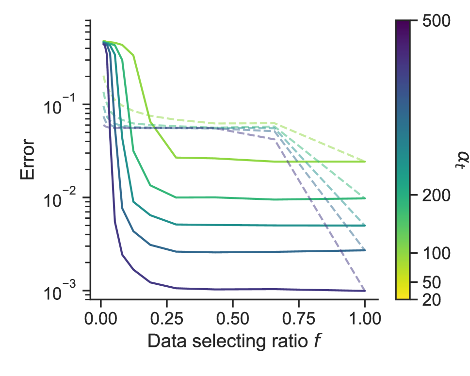
(a) Compare the selection of difficult and simple samples.

(b) Compare hard sample selection and random selection.

Figure 7: The relationship between fitting error and $f$ under different difficulty sample selections. The solid line represents selecting the most difficult sample, the dotted line represents random selection, and the dashed line represents the simplest sample. It can be observed that when the total data size is large, selecting more difficult samples can significantly reduce errors at smaller $f$ values.

In this section, we demonstrated the error $e$ of the model under different data selection ratios $f$ when selecting difficult samples, easy samples(with the largest margin), and random samples with a constant total data volume $\alpha_{t}$ through numerical calculations.

From Figure 7, it can be seen that for values of $f$ that are not too small, selecting hard samples yields better results compared to choosing simple samples or randomly selected samples. This experimental result further explains why we chose hard examples in the main text instead of simple or random selections. We also observed that when $f$ is small, the effectiveness of selecting difficult samples is worse than the other two selection methods.

References

- Bai et al. (2024) Bai, T.; Liang, H.; Wan, B.; Yang, L.; Li, B.; Wang, Y.; Cui, B.; He, C.; Yuan, B.; and Zhang, W. 2024. A Survey of Multimodal Large Language Model from A Data-centric Perspective. CoRR, abs/2405.16640.
- Binici et al. (2022) Binici, K.; Pham, N. T.; Mitra, T.; and Leman, K. 2022. Preventing catastrophic forgetting and distribution mismatch in knowledge distillation via synthetic data. In Proceedings of the IEEE/CVF winter conference on applications of computer vision, 663–671.
- Borgli et al. (2020) Borgli, H.; Thambawita, V.; Smedsrud, P. H.; Hicks, S.; Jha, D.; Eskeland, S. L.; Randel, K. R.; Pogorelov, K.; Lux, M.; Nguyen, D. T. D.; Johansen, D.; Griwodz, C.; Stensland, H. K.; Garcia-Ceja, E.; Schmidt, P. T.; Hammer, H. L.; Riegler, M. A.; Halvorsen, P.; and de Lange, T. 2020. HyperKvasir, a comprehensive multi-class image and video dataset for gastrointestinal endoscopy. Scientific Data, 7(1): 283.
- Cazenavette et al. (2022) Cazenavette, G.; Wang, T.; Torralba, A.; Efros, A. A.; and Zhu, J.-Y. 2022. Dataset distillation by matching training trajectories. In Proceedings of the IEEE/CVF Conference on Computer Vision and Pattern Recognition, 4750–4759.
- Ceccarello, Pietracaprina, and Pucci (2018) Ceccarello, M.; Pietracaprina, A.; and Pucci, G. 2018. Fast coreset-based diversity maximization under matroid constraints. In Proceedings of the Eleventh ACM International Conference on Web Search and Data Mining, 81–89.
- Contributors (2020) Contributors, M. 2020. MMSegmentation: OpenMMLab Semantic Segmentation Toolbox and Benchmark. https://github.com/open-mmlab/mmsegmentation.
- Dosovitskiy et al. (2020) Dosovitskiy, A.; Beyer, L.; Kolesnikov, A.; Weissenborn, D.; Zhai, X.; Unterthiner, T.; Dehghani, M.; Minderer, M.; Heigold, G.; Gelly, S.; Uszkoreit, J.; and Houlsby, N. 2020. An Image is Worth 16x16 Words: Transformers for Image Recognition at Scale. CoRR, abs/2010.11929.
- Feldman and Zhang (2020) Feldman, V.; and Zhang, C. 2020. What Neural Networks Memorize and Why: Discovering the Long Tail via Influence Estimation. In Larochelle, H.; Ranzato, M.; Hadsell, R.; Balcan, M.; and Lin, H., eds., Advances in Neural Information Processing Systems 33: Annual Conference on Neural Information Processing Systems 2020, NeurIPS 2020, December 6-12, 2020, virtual.
- Gotmare et al. (2018) Gotmare, A.; Keskar, N. S.; Xiong, C.; and Socher, R. 2018. A closer look at deep learning heuristics: Learning rate restarts, warmup and distillation. arXiv preprint arXiv:1810.13243.
- Guo et al. (2023) Guo, Z.; Wang, K.; Cazenavette, G.; Li, H.; Zhang, K.; and You, Y. 2023. Towards lossless dataset distillation via difficulty-aligned trajectory matching. arXiv preprint arXiv:2310.05773.
- He et al. (2022) He, K.; Chen, X.; Xie, S.; Li, Y.; Dollár, P.; and Girshick, R. 2022. Masked Autoencoders Are Scalable Vision Learners. In Proceedings of the IEEE/CVF Conference on Computer Vision and Pattern Recognition (CVPR), 16000–16009.
- Ji, Heo, and Park (2021) Ji, M.; Heo, B.; and Park, S. 2021. Show, attend and distill: Knowledge distillation via attention-based feature matching. In Proceedings of the AAAI Conference on Artificial Intelligence, volume 35, 7945–7952.
- Killamsetty et al. (2021) Killamsetty, K.; Sivasubramanian, D.; Ramakrishnan, G.; De, A.; and Iyer, R. K. 2021. GRAD-MATCH: Gradient Matching based Data Subset Selection for Efficient Deep Model Training. In Meila, M.; and Zhang, T., eds., Proceedings of the 38th International Conference on Machine Learning, ICML 2021, 18-24 July 2021, Virtual Event, volume 139 of Proceedings of Machine Learning Research, 5464–5474. PMLR.
- Kirillov et al. (2023) Kirillov, A.; Mintun, E.; Ravi, N.; Mao, H.; Rolland, C.; Gustafson, L.; Xiao, T.; Whitehead, S.; Berg, A. C.; Lo, W.-Y.; Dollar, P.; and Girshick, R. 2023. Segment Anything. In Proceedings of the IEEE/CVF International Conference on Computer Vision (ICCV), 4015–4026.
- Kolides et al. (2023) Kolides, A.; Nawaz, A.; Rathor, A.; Beeman, D.; Hashmi, M.; Fatima, S.; Berdik, D.; Al-Ayyoub, M.; and Jararweh, Y. 2023. Artificial intelligence foundation and pre-trained models: Fundamentals, applications, opportunities, and social impacts. Simulation Modelling Practice and Theory, 126: 102754.
- Lei and Tao (2023) Lei, S.; and Tao, D. 2023. A comprehensive survey of dataset distillation. IEEE Transactions on Pattern Analysis and Machine Intelligence.
- Loo et al. (2023) Loo, N.; Hasani, R. M.; Lechner, M.; and Rus, D. 2023. Dataset Distillation with Convexified Implicit Gradients. CoRR, abs/2302.06755.
- Loshchilov and Hutter (2017) Loshchilov, I.; and Hutter, F. 2017. Decoupled Weight Decay Regularization.
- Ma et al. (2021) Ma, Y.; Chen, X.; Cheng, K.; Li, Y.; and Sun, B. 2021. LDPolypVideo Benchmark: A Large-Scale Colonoscopy Video Dataset of Diverse Polyps. In de Bruijne, M.; Cattin, P. C.; Cotin, S.; Padoy, N.; Speidel, S.; Zheng, Y.; and Essert, C., eds., Medical Image Computing and Computer Assisted Intervention – MICCAI 2021, 387–396. Cham: Springer International Publishing. ISBN 978-3-030-87240-3.
- Meding et al. (2022) Meding, K.; Buschoff, L. M. S.; Geirhos, R.; and Wichmann, F. A. 2022. Trivial or Impossible — dichotomous data difficulty masks model differences (on ImageNet and beyond). In The Tenth International Conference on Learning Representations, ICLR 2022, Virtual Event, April 25-29, 2022. OpenReview.net.
- Mirzasoleiman, Bilmes, and Leskovec (2020) Mirzasoleiman, B.; Bilmes, J. A.; and Leskovec, J. 2020. Coresets for Data-efficient Training of Machine Learning Models. In Proceedings of the 37th International Conference on Machine Learning, ICML 2020, 13-18 July 2020, Virtual Event, volume 119 of Proceedings of Machine Learning Research, 6950–6960. PMLR.
- Nguyen, Chen, and Lee (2021) Nguyen, T.; Chen, Z.; and Lee, J. 2021. Dataset Meta-Learning from Kernel Ridge-Regression. In 9th International Conference on Learning Representations, ICLR 2021, Virtual Event, Austria, May 3-7, 2021. OpenReview.net.
- Nguyen et al. (2021) Nguyen, T.; Novak, R.; Xiao, L.; and Lee, J. 2021. Dataset Distillation with Infinitely Wide Convolutional Networks. In Ranzato, M.; Beygelzimer, A.; Dauphin, Y. N.; Liang, P.; and Vaughan, J. W., eds., Advances in Neural Information Processing Systems 34: Annual Conference on Neural Information Processing Systems 2021, NeurIPS 2021, December 6-14, 2021, virtual, 5186–5198.
- Paul, Ganguli, and Dziugaite (2021) Paul, M.; Ganguli, S.; and Dziugaite, G. K. 2021. Deep Learning on a Data Diet: Finding Important Examples Early in Training. In Ranzato, M.; Beygelzimer, A.; Dauphin, Y. N.; Liang, P.; and Vaughan, J. W., eds., Advances in Neural Information Processing Systems 34: Annual Conference on Neural Information Processing Systems 2021, NeurIPS 2021, December 6-14, 2021, virtual, 20596–20607.
- Pooladzandi, Davini, and Mirzasoleiman (2022) Pooladzandi, O.; Davini, D.; and Mirzasoleiman, B. 2022. Adaptive Second Order Coresets for Data-efficient Machine Learning. In Chaudhuri, K.; Jegelka, S.; Song, L.; Szepesvári, C.; Niu, G.; and Sabato, S., eds., International Conference on Machine Learning, ICML 2022, 17-23 July 2022, Baltimore, Maryland, USA, volume 162 of Proceedings of Machine Learning Research, 17848–17869. PMLR.
- Ranftl, Bochkovskiy, and Koltun (2021) Ranftl, R.; Bochkovskiy, A.; and Koltun, V. 2021. Vision Transformers for Dense Prediction. In Proceedings of the IEEE/CVF International Conference on Computer Vision (ICCV), 12179–12188.
- Sorscher et al. (2022) Sorscher, B.; Geirhos, R.; Shekhar, S.; Ganguli, S.; and Morcos, A. 2022. Beyond neural scaling laws: beating power law scaling via data pruning. In Koyejo, S.; Mohamed, S.; Agarwal, A.; Belgrave, D.; Cho, K.; and Oh, A., eds., Advances in Neural Information Processing Systems, volume 35, 19523–19536. Curran Associates, Inc.
- Sun et al. (2024) Sun, P.; Shi, B.; Yu, D.; and Lin, T. 2024. On the Diversity and Realism of Distilled Dataset: An Efficient Dataset Distillation Paradigm. In Proceedings of the IEEE/CVF Conference on Computer Vision and Pattern Recognition (CVPR), 9390–9399.
- Toneva et al. (2019) Toneva, M.; Sordoni, A.; des Combes, R. T.; Trischler, A.; Bengio, Y.; and Gordon, G. J. 2019. An Empirical Study of Example Forgetting during Deep Neural Network Learning. In 7th International Conference on Learning Representations, ICLR 2019, New Orleans, LA, USA, May 6-9, 2019. OpenReview.net.
- Wang et al. (2018) Wang, T.; Zhu, J.; Torralba, A.; and Efros, A. A. 2018. Dataset Distillation. CoRR, abs/1811.10959.
- Xu et al. (2020) Xu, Y.; Zhao, S.; Song, J.; Stewart, R.; and Ermon, S. 2020. A Theory of Usable Information Under Computational Constraints. CoRR, abs/2002.10689.
- Xu et al. (2023) Xu, Z.; Chen, Y.; Pan, M.; Chen, H.; Das, M.; Yang, H.; and Tong, H. 2023. Kernel ridge regression-based graph dataset distillation. In Proceedings of the 29th ACM SIGKDD Conference on Knowledge Discovery and Data Mining, 2850–2861.
- Yang et al. (2024) Yang, W.; Tan, W.; Sun, Y.; and Yan, B. 2024. A Medical Data-Effective Learning Benchmark for Highly Efficient Pre-training of Foundation Models. In ACM Multimedia 2024.
- Zhang et al. (2021) Zhang, B.; Zhang, X.; Liu, Y.; Cheng, L.; and Li, Z. 2021. Matching distributions between model and data: Cross-domain knowledge distillation for unsupervised domain adaptation. In Proceedings of the 59th Annual Meeting of the Association for Computational Linguistics and the 11th International Joint Conference on Natural Language Processing (Volume 1: Long Papers), 5423–5433.
- Zhao, Mopuri, and Bilen (2021) Zhao, B.; Mopuri, K. R.; and Bilen, H. 2021. Dataset Condensation with Gradient Matching. In 9th International Conference on Learning Representations, ICLR 2021, Virtual Event, Austria, May 3-7, 2021. OpenReview.net.