Anatomical Foundation Models for Brain MRIs

Abstract

Deep Learning (DL) in neuroimaging has become increasingly relevant for detecting neurological conditions and neurodegenerative disorders. One of the most predominant biomarkers in neuroimaging is represented by brain age, which has been shown to be a good indicator for different conditions, such as Alzheimer’s Disease. Using brain age for pretraining DL models in transfer learning settings has also recently shown promising results, especially when dealing with data scarcity of different conditions. On the other hand, anatomical information of brain MRIs (e.g. cortical thickness) can provide important information for learning good representations that can be transferred to many downstream tasks. In this work, we propose AnatCL, an anatomical foundation model for brain MRIs that i.) leverages anatomical information with a weakly contrastive learning approach and ii.) achieves state-of-the-art performances in many different downstream tasks. To validate our approach we consider 12 different downstream tasks for diagnosis classification, and prediction of 10 different clinical assessment scores.

1 Introduction

Magnetic Resonance Imaging (MRI) is the foundation of neuroimaging, providing detailed views of brain structure and function that are crucial for diagnosing and understanding various neurological conditions. However, the complexity and high dimensionality of MRI data present significant challenges for automated analysis. Traditional machine learning methods often require extensive manual annotation, which is both time-consuming and expensive. Recently, contrastive deep learning techniques have emerged as powerful tools for extracting meaningful information from complex data, showing promise in improving the automated analysis of neuroimaging datasets.

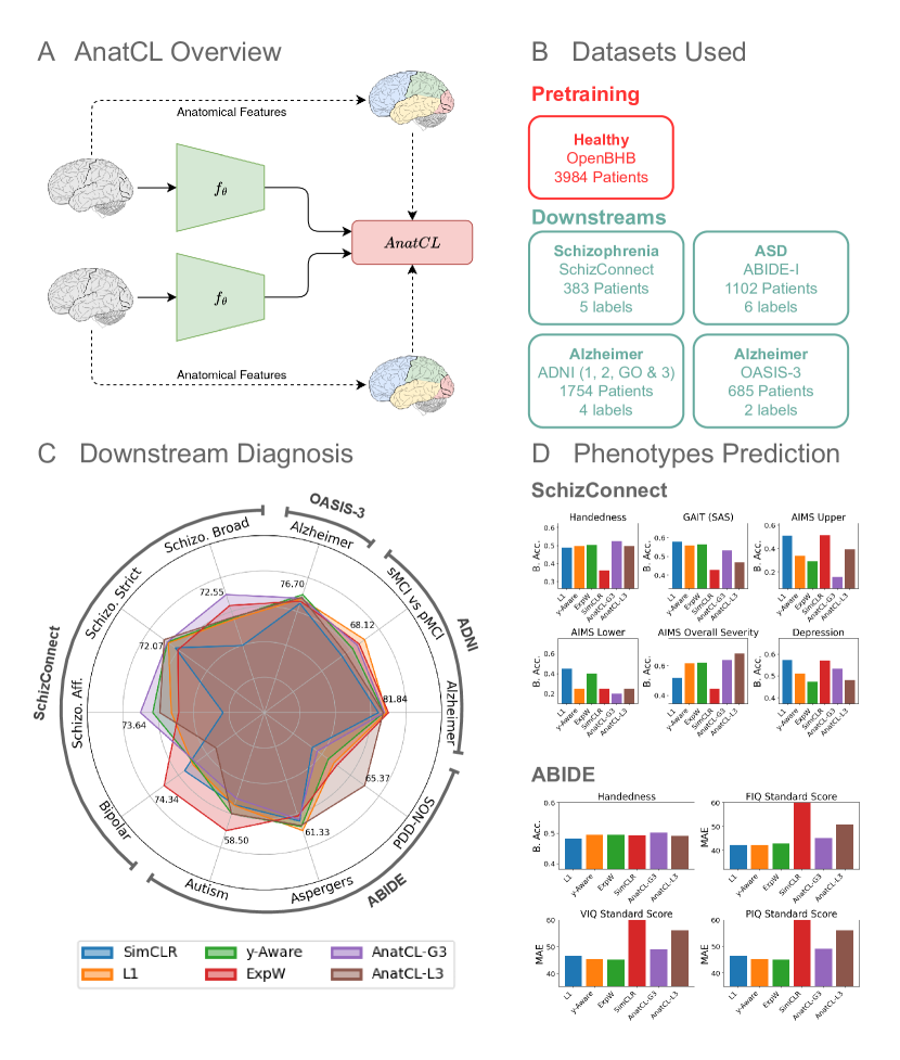
Figure 1: We propose AnatCL, a contrastive approach that leverages anatomical information in brain MRIs in order to learn meaningful and general representation. AnatCL can transfer to different downstream tasks achieving comparable or better results that standard state-of-the-art approaches, which are based on brain age prediction.

Contrastive learning methods, particularly those leveraging supervised contrastive loss functions, have been effective in creating models that learn robust representation spaces. These methods typically utilize metadata, such as patient age, to guide the learning process, with the aim of aligning similar data points (i.e. similar age) and distinguishing dissimilar ones in the representation space. While this approach has yielded promising results, it may fall short of fully capturing the multifaceted information inherent in MRI data and the anatomical complexity of the brain.

For this reason, in this paper, we extend the capabilities of existing contrastive learning approaches by incorporating additional anatomical measures into the loss formulation. We propose AnatCL, a contrastive learning framework that builds upon previous works that leverages patient age as proxy metadata [12, 1] to also include information derived from anatomical measures (such as cortical thickness), computed on region of interests (ROIs) of common atlas such as the Desikan-Killiany parcellation [7] Specifically, we propose a modified contrastive learning loss function that integrates patient age with a targeted selection of three anatomical features: Mean Cortical Thickness, Gray Matter Volume, Surface Area. This selective integration was designed to assess the effectiveness of using potentially more informative anatomical features in conjunction with demographic data.

We propose and test two versions of our framework: a local version that considers the distance between representations as the distance between local measurements in the Desikan format (a set of $68\times 3$ features), and a global version that considers the same three features across all Desikan regions ($3\times 68$ features). The local version aims to capture the localized anatomical variations within specific regions, while the global version aggregates these features across the entire brain to provide a more holistic view.

An overview of AnatCL is provided by Fig. 1. First, we pretrain our models using the proposed method on the OpenBHB dataset, a large collection of healthy samples, then we test the resulting models on different downstream tasks across a variety of publicly available datasets (Sec. 3.1). Our results indicate that in some downstream tasks, our method can achieve comparable or better results than standard state-of-the-art approaches based on brain age prediction. These findings suggest that incorporating targeted anatomical features alongside patient age in contrastive learning frameworks can enhance the performance of neuroimaging models, leading to the development of models that learn more meaningful and generalizable representation spaces. Additionally, we also perform experiments to check whether anatomical information can be leveraged for predicting phenotypes and clinical assessments scores. To the best of our knowledge, this is one of the first works attempting this. In summary, our contribution is multifold:

1. We propose a novel weakly contrastive learning formulation that is able to take into account multiple features and metadata for guiding the learning process;

2. We propose AnatCL, a foundation models based on both anatomical and demographic features to build robust and generalizeable representations of structural neuroimaging data;

3. We perform extensive validation across 12 different downstream clinical tasks (diagnosis) and prediction of 10 different phenotypes and clinical assessment scores.

Furthermore, we also publicly release our pre-trained models for researchers worldwide at omittedlink.

2 Related Works

Machine learning on structural brain imaging.

Current literature has been mainly devoted to segmentation tasks for brain anatomical data, such as brain tumor segmentation [2] or tissue segmentation [10], in a supervised setting requiring annotated maps. The deep neural network U-Net [25] and its extension nnU-Net [18] were very successful at such tasks. Another body of literature tackled phenotype and clinical prediction tasks from structural imaging, such as age prediction [14], Alzheimer’s disease detection [31], cognitive impairment detection, or psychiatric conditions prediction [22, 4]. Current approaches mostly involve traditional machine learning models such as SVM or penalized linear models trained in a supervised fashion to predict the targeted phenotypes. Since most studies only include a few hundred subjects in their datasets, larger models introducing more parameters (such as neural networks) do not necessarily translate into better performance [11, 26, 16], probably because of over-fitting.

Self-supervised learning on brain imaging.

Self-supervised learning has been popularized by its impressive performance in Natural Language Processing (NLP) using auto-regressive models trained on web-scale text corpus and mainly deployed on generation tasks [8, 3]. Since it does not require a supervised signal for training, it is particularly appealing when large-scale data are available, and the annotation cost is prohibitive. Its applicability on neuroimage data is still unclear and very few studies have tackled this problem so far [17].  [12] demonstrated that contrastive learning integrating subjects meta-data can improve the classification of patients with psychiatric conditions.  [29] demonstrated that learning frameworks from NLP, such as sequence-to-sequence autoencoding, causal language modeling, and masked language modeling, can improve mental state decoding from brain activity recorded with functional MRI.

Contrastive Learning on brain imaging

Recently, interests in contrastive learning approaches for brain age prediction has risen. Among different works we can identify y-Aware [12] and ExpW [1]. These works propose to utilize contrastive learning for continuous regression tasks, by employing a kernel to measure similarity between different samples. In these works, age is used as pre-training target, followed by transfer learning on specific diseases. However, they are limited to only considering age as pretraining feature. In this work, we extend this formulation to work with multiple attributes.

3 Materials and Methods

3.1 Experimental data

We use a collection of T1-weighted MRI scans comprising 7,908 different individuals, for a total of 21,155 images. The experimental data is gathered from different publicly available datasets, and we target 5 different neurological conditions: healthy samples (OpenBHB [13]), Alzheimer’s Disease (ADNI [23] and OASIS-3 [20]), schizophrenia (SchizConnect [30]) and Autism Spectrum Disorder (ABIDE I [9]). The overall composition of the cohorts used in this study is presented in Fig. 1B. Tab. 1 provides an overview of all the downstream tasks that we explore in this work.

OpenBHB

OpenBHB is a recently released dataset that aggregates healthy control (HC) samples from many public cohorts (ABIDE 1, ABIDE 2, CoRR, GSP, IXI, Localizer, MPI-Leipzig, NAR, NPC, RBP). Every scan comes from a different subject. We use OpenBHB as pretraining dataset for our method. Besides the structural scans and patients information, OpenBHB also provides 7 anatomical measures according to the Desikan-Kiliani parcellation [7] (cortical thickness mean and std, gray matter volume, surface area, integrated mean, gaussian curvature index and intrinsic curvature index [13]).

ADNI and OASIS-3

We include all phases ADNI-1, ADNI-2, ADNI-GO and ADNI-3 in our study, amounting to 633 HC, 712 MCI and 409 AD patients. For OASIS3 we include 685 patients respectively, containing 88 AD cases.

SchizConnect

We include anatomical MRIs for a total of 383 patients, divided in 180 HC, 102 with schizophrenia (broad), 74 with schizophrenia (strict), 11 schizoaffective patients and 9 with bipolar disorder.

ABIDE I

We include anatomical MRIs for a total of 1102 patients, divided in 556 HC, 339 patients with autism, 93 patients with Asperger’s Syndrome, and 7 with pervasive developmental disorder not otherwise specified (PDD-NOS).

Clinical assessment scores

In addition to predict the above diagnosis, we also consider some relevant clinical assessment included in the data, as reported in Tab. 1. For SchizConnect, we consider the Abormal Involuntary Movement Scale (AIMS) evaluated in three assessments (overall, uppder body, lower body), a Depression score based on the Calgary Scale, Handedness information, and GAIT measuremens with the Simpson-Angus-Scale (SAS). For ABIDE, we consider also handedness and three IQ scores, namely Full Scale IQ (FIQ), Visual IQ (VIQ) and Performance IQ (FIQ) measured with the Wechsler Abbreviated Scale (WASI).

Table 1: Summary of downstream tasks (12) and clinical assessment scores (10) considered in the study.

Dataset	Task / Condition
OpenBHB	Age (HC)
	Sex
ADNI	Alzheimer’s Disease
	sMCI vs pMCI
OASIS-3	Alzheimer’s Disease
SchizConnect	Schizophrenia Broad
	Schizophrenia Strict
	Bipolar Disorder
	Schizoaffective
ABIDE I	Autism
	Aspergers
	PDD-NOS

Dataset	Phenotype
SchizConnect	AIMS Overall Severity
	AIMS Upper Body
	AIMS Lower Body
	Depression
	Handedness
	SAS GAIT
ABIDE 1	Handedness
	FIQ (WASI)
	VIQ (WASI)
	PIQ (WASI)

3.1.1 Data preparation and preprocessing

All the images underwent the same standard VBM preprocessing, using CAT12 [15], which includes non-linear registration to the MNI template and gray matter (GM) extraction. The final spatial resolution is 1.5mm isotropic and the images are of size 121 x 145 x 121. The preprocessing is performed using the brainprep package . After preprocessing, we consider in this work modulated gray matter (GM) images, as in [13].

3.2 Background

Contrastive learning (CL) (either self-supervised as in SimCLR [5] or supervised as in SupCon [19]) leverages discrete labels (i.e., categories) to define positive and negative samples. Starting from a sample $x$, called the anchor, and its latent representation $z=f(x)$, CL approaches aim at aligning the representations of all positive samples to $z$, while repelling the representations of the negative ones. CL is thus not adapted for regression (i.e., continuous labels), as a hard boundary between positive and negative samples cannot be determined. Recently, there have been developments in the field of CL for tackling regression problems, especially aimed at brain age prediction, such as y-Aware [12] and ExpW [1], from brain MRIs. These approaches can be broadly categorized as weakly contrastive, as brain age is used as pre-train task.

3.3 Weakly contrastive learning

To tackle the issue of continuous labels, weakly contrastive approaches employ the notion of a degree of “positiveness” between samples. This degree is usually defined by a kernel function $w_{i}=K(y-y_{i})$, where $0\leq w_{i}\leq 1$ is computed by a Gaussian or a Radial Basis Function (RBF) kernel and $y,y_{i}$ are the continuous attributes of interest. The goal of weakly contrastive learning is thus to learn a parametric function $f:\mathcal{X}\rightarrow\mathbb{S}^{d}$ that maps samples with a high degree of positiveness ($w_{i}\sim 1$) close in the latent space and samples with a low degree ($w_{i}\sim 0$) far away from each other. y-Aware [12] proposes to do so by aligning positive samples with a strength proportional to the degree, i.e.:

$$\mathcal{L}^{y-aware}=-\sum_{i}\frac{w_{i}}{\sum_{j}w_{j}}\log\left(\frac{\exp(sim(f(x),f(x_{i}))}{\sum_{t=1}^{N}\exp(sim(f(x),f(x_{t})))}\right)$$ (1)

where $sim$ is a similarity function (e.g. cosine). A similar approach is also adopted by ExpW [1]. A limitation of this class of approaches is the reliance on one single attribute (age) to determine the alignment strength. They are thus not suited to leverage multiple attributes (e.g. anatomical measurements of the brain). Our proposed approach aims to solve this issue by extending the weakly contrastive formulation to include multiple attributes.

3.4 Proposed method

In this section, we will discuss our approach to include multiple attributes in a weakly contrastive paradigm.

3.4.1 Anatomical Contrastive Learning with anatomical measures

We propose a novel formulation for weakly contrastive learning to employ multiple anatomical attributes derived from the MRI scan, that we call AnatCL. The features we consider are derived from the standard Desikan-Kiliany parcellation [7], based on the information available in the OpenBHB dataset (see Sec. 3.1). Among the anatomical measurements, we consider cortical thickness (CT), gray matter volume (GMV), and surface area (SA) [13]. To include these measurements inside AnatCL, we propose two different formulation, global and local, based on how the similarity across two brain scans is computed.

Local Descriptor

For each of the 68 regions, we obtain a local anatomical descriptor $\psi^{k}\in\mathbb{R}^{3}$ where $k\in\{1,\dots,68\}$ composed by the three anatomical measurements considered for that specific region. In order to compute the degree of positiveness $w_{i}$ across two samples $x$ and $x_{i}$, given their corresponding anatomical descriptors $\Psi=\{\psi^{1},\dots\,\psi^{68}\}$ and $\Psi_{i}=\{\psi^{1}_{i},\dots\,\psi^{68}_{i}\}$ we compute the average cross-region similarity (which we call local descriptor) as:

$$w_{i}=\frac{1}{68}\sum_{k=1}^{68}K(\gamma(\psi^{k}),\gamma(\psi^{k}_{i}))$$ (2)

where $K$ can either be a similarity function or a kernel as in [12], and $\gamma(x)$ is a normalization that normalizes each component of $x$ to a standard range $[0,1]$. In this work, for simplicity, we choose to employ cosine similarity as $K$.

Global Descriptor

Taking a complementary approach, we now consider global anatomy descriptors $\omega^{k}\in\mathbb{R}^{68}$ for the entire brain with $k\in\{1,2,3\}$, that contain the values across all 68 regions for each anatomical measurement. Similarly to above, in order to compute the degree of positiveness $w_{i}$ between two samples $x$ and $x_{i}$ given their global anatomical descriptors $\Omega=\{\omega^{1},\dots,\omega^{3}\}$ and $\Omega_{i}=\{\omega^{1}_{i},\dots,\omega^{3}_{i}\}$ we compute the cross-measurement similarity (global descriptor) as:

$$w_{i}=\frac{1}{3}\sum_{k=1}^{3}K(\omega^{k},\omega^{k}_{i})$$ (3)

This time we do not need to standardize $\omega^{k}$ and $\omega^{k}_{i}$ as $K$ is evaluated between features of the same type, so the scale of the value is comparable. Also in this case, for the sake of simplicity, we employ a cosine similarity function for $K$.

Our proposed AnatCL loss function is based on y-Aware [12] and integrates the computed $w_{i}$ (either local or global) as in Eq. 1.

3.4.2 Final objective function

For training, we also consider the available age information, thus our final loss formulation becomes:

$$\mathcal{L}=\lambda_{1}\mathcal{L}_{age}+\lambda_{2}\mathcal{L}_{AnatCL}$$ (4)

where $\mathcal{L}_{age}$ is defined as in Eq. 1 and $\mathcal{L}_{AnatCL}$ is defined as in Sec. 3.4.1. It is worth noting that the considered anatomical features in AnatCL can be computed directly from the 3D MRI with standard tools such as FreeSurfer , and thus our method does not require any additional label in the dataset.

4 Results

In this section, we present the results of our proposed method in comparison to existing state-of-the-art approaches in several downstream task.

4.1 Experimental setup

Our experiments involved pretraining a model using the proposed AnatCL loss on the OpenBHB dataset, followed by testing the resulting model on various downstream tasks across different datasets. The experimental settings for the two loss formulations, local (AnatCL-G3) and global (AnatCL-L3), are identical. We pretrain two ResNet-18 3D models using VBM-preprocessed images and their corresponding Desikan measures with the proposed formulations. The training process employs the Adam optimizer with a learning rate of 0.0001, and a decay rate of 0.9 applied after every 10 epochs. The models are trained with a batch size of 32 for a total of 300 epochs. As values of $\lambda_{1}$ and $\lambda_{2}$, for simplicity, we use 1. As standard practice in CL approaches [5, 19], the contrastive loss is computed on a fully-connected projection head following the encoder, composed of two layers. To ensure robust evaluation, we perform cross-validation using 5 folds. The results are computed in terms of mean and standard deviation across the 5 folds.

After the pre-training step we evaluate the models by testing their performance with a transfer learning approach: we extract the latent representations generated by the model using only the encoder of the model (i.e., discarding the fully connected head). For each downstream task, we train different linear classifiers on the extracted representations to assess the model’s ability to learn meaningful and generalizable features.

For comparison with standard approaches, we also implement four different baselines: SimCLR [5] (completely self-supervised) and three supervised baselines: a standard model trained with the L1 loss, y-Aware [12] and ExpW [1] which has shown state-of-the-art results on the OpenBHB challenge [13]. For all these methods, we follow the same experimental setup described above.

To run our experiments, we employ a cluster of 4 NVIDIA V100 GPUs, with a single training taking around 10h.

4.2 Brain age prediction

Preliminary results in terms of brain age prediction and sex classification are evaluated on the OpenBHB dateset. The results are reported in Tab. 2. From the results we conclude that AnatCL is able to match and slightly surpass state-of-the-art performance on brain age prediction. It is worth noting that we do not employ any bias-correction method as in [6, 21]. For sex classification, we do not match ExpW [1], but we improve over the SimCLR and L1 baselines.

Table 2: Results on OpenBHB in terms of mean absolute error (MAE) on age prediction, and balanced accuracy on sex classification.

Model	Method	Age MAE	Sex
ResNet-18	SimCLR [5]	5.58$\pm$0.53	76.7$\pm$1.67
	L1 (age supervised)	2.73$\pm$0.14	76.7$\pm$0.67
	y-Aware [12]	2.66$\pm$0.06	79.6$\pm$1.13
	ExpW [1]	2.70$\pm$0.06	80.3$\pm$1.7
	AnatCL-G3	2.61$\pm$0.08	78.2$\pm$1.25
	AnatCL-L3	2.64$\pm$0.07	78.2$\pm$0.7

4.3 Alzheimer’s desease and cognitive impariments

Table 3: Results on Alzheimer’s Disease (AD) classification in terms of balanced accuracy.

		ADNI		OASIS-3
Model	Method	HC vs AD	sMCI vs pMCI	HC vs AD
ResNet-18	SimCLR [5]	78.47$\pm$2.51	61.77$\pm$3.85	73.97$\pm$4.98
	L1 (age supervised)	81.20$\pm$2.3	68.12$\pm$5.42	75.40$\pm$5.4
	y-Aware [12]	80.3$\pm$1.8	64.72$\pm$4.43	76.70$\pm$3.30
	ExpW [1]	81.84$\pm$2.95	66.54$\pm$5.64	74.67$\pm$2.87
	AnatCL-G3	80.47$\pm$2.95	66.03$\pm$2.93	75.59$\pm$2.67
	AnatCL-L3	80.11$\pm$1.0	62.83$\pm$4.5	75.88$\pm$3.0

In Tab. 3 we report results for Alzheimer’s Disease (AD) detection on ADNI and OASIS-3. While we do not reach the best results overall, AnatCL can usually improve over the self-supervised baseline (SimCLR) and sometimes over either L1, y-Aware or ExpW.

4.4 Schizophrenia and ASD

We evaluate downstream performance on SchizConnect for detecting schizophrenia (broad and strict), schizoaffective and bipolar patients. Results are reported in Tab. 4. With AnatCL we achieve state-of-the-art performance on three out of four tasks, denoting that taking anatomical information into account can prove useful for these psychiatric conditions. We also assess detection performance for Autism Spectrum Disorder (ASD) patients, across three categories (autism, aspergers and PDD-NOS), results are reported in Tab. 4. While AnatCL does not beat the other methods on autistic and aspergers patients, we significantly improve the accuracy for PDD-NOS patients, which is a rarer diagnosis in the data. Overall, AnatCL is able to more consistently achieve improved results than any other baseline.

Table 4: Results on schizophrenia detection (SCZ) and autism spectrum disorder (ASD) in terms of balanced accuracy.

		Schizconnect				ABIDE-I
Model	Method	SCZ. (Broad)	SCZ (Strict)	Schizoaff.	Bipolar	Autism	Aspergers	PDD-NOS
ResNet-18	SimCLR [5]	58.53$\pm$3.52	68.47$\pm$8.47	51.23$\pm$11.94	67.34$\pm$9.96	54.45$\pm$2.99	59.61$\pm$2.72	52.12$\pm$6.62
	L1	65.79$\pm$4.74	70.68$\pm$5.10	65.24$\pm$15.21	64.49$\pm$22.08	54.53$\pm$1.79	61.33$\pm$8.77	57.54$\pm$5.93
	y-Aware [12]	66.20$\pm$4.50	71.04$\pm$2.31	70.29$\pm$14.73	63.95$\pm$19.81	55.84$\pm$3.37	60.60$\pm$9.22	56.17$\pm$10.17
	ExpW [1]	69.53$\pm$4.43	67.65$\pm$8.27	63.26$\pm$18.06	74.34$\pm$18.95	58.50$\pm$2.41	58.68$\pm$3.82	58.31$\pm$4.33
	AnatCL-G3	72.55$\pm$5.16	71.03$\pm$8.53	73.65$\pm$7.29	63.43$\pm$15.94	53.48$\pm$0.99	59.32$\pm$6.58	53.38$\pm$5.86
	AnatCL-L3	66.38$\pm$5.96	72.07$\pm$8.42	68.37$\pm$8.60	56.60$\pm$11.48	55.85$\pm$1.02	60.40$\pm$2.29	65.37$\pm$6.73

4.5 Cognitive score / assessments

As final experiments, we turn our attention to predicting clinical assessments score from brain MRIs. To the best of our knowledge, this has not been explored in other works, and it could provide useful insights on the relation between brain anatomy and behavioral phenotypes. The 10 phenotypes considered can be distinguished based on the prediction task: AIMS, depression, handedness and GAIT are classification tasks, while IQ scores (FIQ, VIQ and PIQ) are regression tasks. For handendess, we predict right-handed vs other (left-handed or ambi), for depression we classify between absent vs mild and above, for AIMS we classify between none and minimal vs mild and above, for GAIT between normal vs everything else. For more detailed explanation of the possible value in the considered phenotypes we refer to the official documentation.

Table 5: Assessment scores / phenotypes prediction from brain MRIs.

	SchizConnect						ABIDE
Method	AIMS Overall	AIMS Up.	AIMS Low.	Depression	Handedness	GAIT	Handedness	FIQ (MAE)	VIQ (MAE)	PIQ (MAE)
SimCLR	44.33$\pm$29.92	51.67$\pm$16.16	25.00$\pm$27.39	56.93$\pm$13.88	36.06$\pm$2.72	42.83$\pm$9.61	49.26$\pm$5.78	84.65$\pm$16.36	89.07$\pm$15.14	89.68$\pm$15.00
L1	51.83$\pm$24.43	50.83$\pm$20.82	45.00$\pm$33.17	57.17$\pm$13.06	48.91$\pm$5.60	57.73$\pm$8.64	48.18$\pm$9.43	42.16$\pm$31.17	46.54$\pm$32.57	46.64$\pm$32.24
y-Aware	61.83$\pm$15.87	34.17$\pm$11.90	25.00$\pm$27.39	51.09$\pm$5.32	49.71$\pm$7.69	55.92$\pm$9.52	49.45$\pm$1.56	42.10$\pm$31.14	45.38$\pm$33.19	45.35$\pm$32.76
ExpW	62.00$\pm$12.40	29.17$\pm$17.08	40.00$\pm$33.91	47.26$\pm$7.27	50.39$\pm$6.28	56.39$\pm$14.14	49.53$\pm$3.26	42.94$\pm$30.76	45.28$\pm$33.23	45.02$\pm$32.88
AnatCL-G3	64.00$\pm$12.72	15.83$\pm$12.19	20.00$\pm$18.71	53.35$\pm$8.54	52.44$\pm$9.14	53.10$\pm$11.69	50.21$\pm$6.82	45.18$\pm$29.68	49.07$\pm$31.52	49.30$\pm$30.86
AnatCL-L3	68.50$\pm$18.09	39.17$\pm$14.81	25.00$\pm$27.39	48.05$\pm$10.89	49.67$\pm$8.06	46.74$\pm$5.05	49.13$\pm$3.32	50.77$\pm$27.14	56.18$\pm$28.06	56.13$\pm$27.62

The results are reported in Tab. 5. While we cannot conclude that any of the analysed method can accurately predict all clinical assessments from MRI scans, AnatCL overall achieves the best results three out of ten times, which is more than any other baseline. Interestingly, AnatCL can better predict the overall AIMS score and patients’ handedness, hinting that brain anatomy may be linked with these phenotypes.

5 Limitations, impact and ethical considerations

We believe that foundation models for neuroimaging may have a considerable impact on accurately diagnosing neurological and psyhicatric diseases. With AnatCL we aim at laying the foundations for this path. Currently, AnatCL is limited towards using a single data modality (structural MRI), considering limited anatomical features (only CT, GMV, and SA) and to a relatively small backbone (ResNet-18). Future research should focus on improving these issues, in order to obtain even more accurate predictions. Altough, deep learning techniques can be used in a variety of contexts, we do not believe that AnatCL inherently poses any ethical issue. Furthermore, all the data employed in this work is publicly available for researchers.

6 Conclusions

We propose AnatCL, a foundation model based on brain anatomy and trained with a weakly contrastive learning approach. With thorough validation on 10 different downstream tasks, we show that incorporating anatomy information during training can results in more accurate predictions of different neurological and psychiatry conditions, and also partially clinical assessment scores and phenotypes. We release the weights of the trained model for public use at omittedlink, empowering researchers and practitioners worldwide to leverage AnatCL in many different applications.

Appendix A Anatomical Features

A.1 Details on preprocessing

Anatomical measurements on OpenBHB are released as part of the original dataset. All details can be found in [13]. For preprocessing, the brainprep module was employed, with FreeSurfer version FSL-6.0.5.1, and Desikan-Killiany atlas as provided in FreeSurfer.

A.2 Choice of Anatomical Features

OpenBHB provides 7 different anatomical measures, computed with FreeSurfer: Cortical Thickness (CT, mean and std values), Gray Matter Volume (GMV), Surface Area, Integrated Mean, Gaussian Curvature Index, and Intrinsic Curvature Index. In order to select the most relevant features, we conduct a preliminary study by training a simple linear model (Ridge regression) over each feature, with the task of brain age prediction on the OpenBHB data. The results are evaluated in terms of negative mean absolute error and $R^{2}$ score, and are reported in Tab. 6. The best results are achieved by GVM and Surface Area, which are morphological features regarding the volume and the total area of each ROI. Thus, we select these two features for our experiments with AnatCL. In addition to GMV and Surface Area measures, we also include CT as it is a widely used measure in related works [27, 28]. The final choice is thus composed of three features, which cover different aspects of the morphology and geometry of brain ROIs (e.g. cortical thickness is relevant for conditions such as Alzheimer’s Disease [24], and volume and surface measurements can signal brain atrophy, linked to different conditions).

Table 6: Preliminary study on anatomical features with Ridge regression.

	CT (mean)	GMV	Surf. Area	Int. Mean	Gauss. Curv. Index	Intr. Curv. Index
Neg. MAE	-8.57$\pm$0.03	-6.96$\pm$0.02	-6.93$\pm$0.02	-7.76$\pm$0.01	-8.27$\pm$0.03	-8.36$\pm$0.02
$R^{2}$	0.32$\pm$0.00	0.55$\pm$0.00	0.55$\pm$0.00	0.46$\pm$0.00	0.14$\pm$0.02	0.32$\pm$0.00

References

- [1] Carlo Alberto Barbano, Benoit Dufumier, Edouard Duchesnay, Marco Grangetto, and Pietro Gori. Contrastive learning for regression in multi-site brain age prediction. In 2023 IEEE 20th International Symposium on Biomedical Imaging (ISBI), pages 1–4. IEEE, 2023.
- [2] Erena Siyoum Biratu, Friedhelm Schwenker, Yehualashet Megersa Ayano, and Taye Girma Debelee. A survey of brain tumor segmentation and classification algorithms. Journal of Imaging, 7(9):179, 2021.
- [3] Tom Brown, Benjamin Mann, Nick Ryder, Melanie Subbiah, Jared D Kaplan, Prafulla Dhariwal, Arvind Neelakantan, Pranav Shyam, Girish Sastry, Amanda Askell, et al. Language models are few-shot learners. Advances in neural information processing systems, 33:1877–1901, 2020.
- [4] Ganesh B Chand, Dominic B Dwyer, Guray Erus, Aristeidis Sotiras, Erdem Varol, Dhivya Srinivasan, Jimit Doshi, Raymond Pomponio, Alessandro Pigoni, Paola Dazzan, et al. Two distinct neuroanatomical subtypes of schizophrenia revealed using machine learning. Brain, 143(3):1027–1038, 2020.
- [5] Ting Chen, Simon Kornblith, Mohammad Norouzi, and Geoffrey Hinton. A simple framework for contrastive learning of visual representations. In International conference on machine learning, pages 1597–1607. PMLR, 2020.
- [6] Irene Cumplido-Mayoral, Marina García-Prat, Grégory Operto, Carles Falcon, Mahnaz Shekari, Raffaele Cacciaglia, Marta Milà-Alomà, Luigi Lorenzini, Silvia Ingala, Alle Meije Wink, Henk JMM Mutsaerts, Carolina Minguillón, Karine Fauria, José Luis Molinuevo, Sven Haller, Gael Chetelat, Adam Waldman, Adam J Schwarz, Frederik Barkhof, Ivonne Suridjan, Gwendlyn Kollmorgen, Anna Bayfield, Henrik Zetterberg, Kaj Blennow, Marc Suárez-Calvet, Verónica Vilaplana, and Juan Domingo Gispert. Biological brain age prediction using machine learning on structural neuroimaging data: Multi-cohort validation against biomarkers of alzheimer’s disease and neurodegeneration stratified by sex. eLife, 12, 4 2023.
- [7] Rahul S Desikan, Florent Ségonne, Bruce Fischl, Brian T Quinn, Bradford C Dickerson, Deborah Blacker, Randy L Buckner, Anders M Dale, R Paul Maguire, Bradley T Hyman, et al. An automated labeling system for subdividing the human cerebral cortex on mri scans into gyral based regions of interest. Neuroimage, 31(3):968–980, 2006.
- [8] Jacob Devlin, Ming-Wei Chang, Kenton Lee, and Kristina Toutanova. Bert: Pre-training of deep bidirectional transformers for language understanding. arXiv preprint arXiv:1810.04805, 2018.
- [9] Adriana Di Martino et al. ABIDE — fcon_1000.projects.nitrc.org. https://fcon_1000.projects.nitrc.org/indi/abide/abide_I.html. [Accessed 22-05-2024].
- [10] Lingraj Dora, Sanjay Agrawal, Rutuparna Panda, and Ajith Abraham. State-of-the-art methods for brain tissue segmentation: A review. IEEE reviews in biomedical engineering, 10:235–249, 2017.
- [11] Benoit Dufumier, Pietro Gori, Sara Petiton, Robin Louiset, Jean-François Mangin, Antoine Grigis, and Edouard Duchesnay. Exploring the potential of representation and transfer learning for anatomical neuroimaging: application to psychiatry. HAL, 2024.
- [12] Benoit Dufumier, Pietro Gori, Julie Victor, Antoine Grigis, Michele Wessa, Paolo Brambilla, Pauline Favre, Mircea Polosan, Colm Mcdonald, Camille Marie Piguet, et al. Contrastive learning with continuous proxy meta-data for 3d mri classification. In Medical Image Computing and Computer Assisted Intervention–MICCAI 2021: 24th International Conference, Strasbourg, France, September 27–October 1, 2021, Proceedings, Part II 24, pages 58–68. Springer, 2021.
- [13] Benoit Dufumier, Antoine Grigis, Julie Victor, Corentin Ambroise, Vincent Frouin, and Edouard Duchesnay. Openbhb: a large-scale multi-site brain mri data-set for age prediction and debiasing. NeuroImage, 263:119637, 2022.
- [14] Katja Franke and Christian Gaser. Ten years of brainage as a neuroimaging biomarker of brain aging: what insights have we gained? Frontiers in neurology, 10:454252, 2019.
- [15] Christian Gaser, Robert Dahnke, Paul M Thompson, Florian Kurth, Eileen Luders, and Alzheimer’s Disease Neuroimaging Initiative. Cat–a computational anatomy toolbox for the analysis of structural mri data. biorxiv, pages 2022–06, 2022.
- [16] Tong He, Ru Kong, Avram J Holmes, Minh Nguyen, Mert R Sabuncu, Simon B Eickhoff, Danilo Bzdok, Jiashi Feng, and BT Thomas Yeo. Deep neural networks and kernel regression achieve comparable accuracies for functional connectivity prediction of behavior and demographics. NeuroImage, 206:116276, 2020.
- [17] Shih-Cheng Huang, Anuj Pareek, Malte Jensen, Matthew P Lungren, Serena Yeung, and Akshay S Chaudhari. Self-supervised learning for medical image classification: a systematic review and implementation guidelines. NPJ Digital Medicine, 6(1):74, 2023.
- [18] Fabian Isensee, Paul F Jaeger, Simon AA Kohl, Jens Petersen, and Klaus H Maier-Hein. nnu-net: a self-configuring method for deep learning-based biomedical image segmentation. Nature methods, 18(2):203–211, 2021.
- [19] Prannay Khosla, Piotr Teterwak, Chen Wang, Aaron Sarna, Yonglong Tian, Phillip Isola, Aaron Maschinot, Ce Liu, and Dilip Krishnan. Supervised contrastive learning. Advances in neural information processing systems, 33:18661–18673, 2020.
- [20] Pamela J LaMontagne, Tammie LS Benzinger, John C Morris, Sarah Keefe, Russ Hornbeck, Chengjie Xiong, Elizabeth Grant, Jason Hassenstab, Krista Moulder, Andrei G Vlassenko, et al. Oasis-3: longitudinal neuroimaging, clinical, and cognitive dataset for normal aging and alzheimer disease. MedRxiv, pages 2019–12, 2019.
- [21] Ann-Marie G De Lange and James H Cole. Commentary: Correction procedures in brain-age prediction. 2020.
- [22] Abraham Nunes, Hugo G Schnack, Christopher RK Ching, Ingrid Agartz, Theophilus N Akudjedu, Martin Alda, Dag Alnæs, Silvia Alonso-Lana, Jochen Bauer, Bernhard T Baune, et al. Using structural mri to identify bipolar disorders–13 site machine learning study in 3020 individuals from the enigma bipolar disorders working group. Molecular psychiatry, 25(9):2130–2143, 2020.
- [23] Ronald Carl Petersen, Paul S Aisen, Laurel A Beckett, Michael C Donohue, Anthony Collins Gamst, Danielle J Harvey, CR Jack Jr, William J Jagust, Leslie M Shaw, Arthur W Toga, et al. Alzheimer’s disease neuroimaging initiative (adni) clinical characterization. Neurology, 74(3):201–209, 2010.
- [24] Tony X Phan, Sheena Baratono, William Drew, Aaron M Tetreault, Michael D Fox, R Ryan Darby, Alzheimer’s Disease Neuroimaging Initiative, and Alzheimer’s Disease Metabolomics Consortium. Increased cortical thickness in alzheimer’s disease. Annals of Neurology, 95(5):929–940, 2024.
- [25] Olaf Ronneberger, Philipp Fischer, and Thomas Brox. U-net: Convolutional networks for biomedical image segmentation. In Medical image computing and computer-assisted intervention–MICCAI 2015: 18th international conference, Munich, Germany, October 5-9, 2015, proceedings, part III 18, pages 234–241. Springer, 2015.
- [26] Marc-Andre Schulz, BT Thomas Yeo, Joshua T Vogelstein, Janaina Mourao-Miranada, Jakob N Kather, Konrad Kording, Blake Richards, and Danilo Bzdok. Different scaling of linear models and deep learning in ukbiobank brain images versus machine-learning datasets. Nature communications, 11(1):4238, 2020.
- [27] Saurabh Sihag, Gonzalo Mateos, Corey McMillan, and Alejandro Ribeiro. Explainable brain age prediction using covariance neural networks. Advances in Neural Information Processing Systems, 36, 2024.
- [28] Saurabh Sihag, Gonzalo Mateos, and Alejandro Ribeiro. Towards a foundation model for brain age prediction using covariance neural networks. arXiv preprint arXiv:2402.07684, 2024.
- [29] Armin Thomas, Christopher Ré, and Russell Poldrack. Self-supervised learning of brain dynamics from broad neuroimaging data. Advances in neural information processing systems, 35:21255–21269, 2022.
- [30] Lei Wang, Kathryn I Alpert, Vince D Calhoun, Derin J Cobia, David B Keator, Margaret D King, Alexandr Kogan, Drew Landis, Marcelo Tallis, Matthew D Turner, et al. Schizconnect: Mediating neuroimaging databases on schizophrenia and related disorders for large-scale integration. Neuroimage, 124:1155–1167, 2016.
- [31] Junhao Wen, Elina Thibeau-Sutre, Mauricio Diaz-Melo, Jorge Samper-González, Alexandre Routier, Simona Bottani, Didier Dormont, Stanley Durrleman, Ninon Burgos, Olivier Colliot, et al. Convolutional neural networks for classification of alzheimer’s disease: Overview and reproducible evaluation. Medical image analysis, 63:101694, 2020.