Blessing of Dimensionality for Approximating Sobolev Classes on Manifolds
Abstract
The manifold hypothesis says that natural high-dimensional data is actually supported on or around a low-dimensional manifold. Recent success of statistical and learning-based methods empirically supports this hypothesis, due to outperforming classical statistical intuition in very high dimensions. A natural step for analysis is thus to assume the manifold hypothesis and derive bounds that are independent of any embedding space. Theoretical implications in this direction have recently been explored in terms of generalization of ReLU networks and convergence of Langevin methods. We complement existing results by providing theoretical statistical complexity results, which directly relates to generalization properties. In particular, we demonstrate that the statistical complexity required to approximate a class of bounded Sobolev functions on a compact manifold is bounded from below, and moreover that this bound is dependent only on the intrinsic properties of the manifold. These provide complementary bounds for existing approximation results for ReLU networks on manifolds, which give upper bounds on generalization capacity.
1 Introduction
Data is ever growing, especially in the current era of machine learning. However, dimensionality is not always beneficial, and having too many features can confound simpler underlying truths. This is sometimes referred to as the curse of dimensionality (Altman & Krzywinski, 2018). A classical example is manifold learning, which is known to scale exponentially in the intrinsic dimension (Narayanan & Niyogi, 2009). In the current paradigm of increasing dimensionality, standard statistical tools and machine learning models continue to work, despite the high latent dimensions arising in cases such as computational imaging (Wainwright, 2019). One possible assumption to elucidate this phenomenon comes from the manifold hypothesis, also known as concentration of measure or the blessing of dimensionality (Bengio et al., 2013). This states that real datasets are actually concentrated on or near low-dimensional manifolds, independently of the latent dimension that the data is embedded in.
The manifold hypothesis is generally considered as a theoretical assumption, with empirical studies considering the dimension rather than the construction of the manifold. However, more concrete examples of structure in data have also been considered and exploited (Celledoni et al., 2021). Group equivariance describes how an operation commutes with symmetries in data, such as rotation or reflections in image reconstruction, with applications in unsupervised learning and enforcing faithful neural network reconstructions (Chen et al., 2021; Cohen & Welling, 2016).
Structures can also be found and exploited outside of raw data. Algorithmic structures such as proximal splitting algorithms, arising from convex optimization, are used in Plug-and-Play image reconstruction algorithms (Kamilov et al., 2023; Venkatakrishnan et al., 2013). Learning-to-optimize considers pushing the underlying geometry of the data into corresponding optimization problems, and exploiting common geometry in the function space to achieve significant acceleration in a learned fashion (Andrychowicz et al., 2016; Tan et al., 2023).
In this work, we explore the consequences of the manifold hypothesis through the lens of approximation theory and statistical complexity. For a class of functions with infinite statistical complexity, we consider a nonlinear width in terms of how well it can be approximated in with function classes of finite statistical complexity. This characterizes how close the function class is to having low statistical complexity, motivated by having good sample complexity to learn nearly-optimal functions. We consider how difficult it is to optimally approximate classes of functions with functions of finite statistical complexity in terms of distance. In particular, Theorem 3.1 demonstrates that on a Riemannian manifold, the optimal approximation of a bounded Sobolev class with function classes of finite pseudo-dimension has a rate depending only on the implicit properties of the manifold.
1.1 Related Literature
We detail some literature surrounding the manifold hypothesis, including empirical testing, as well as other theoretical works that show rates that depend mainly on intrinsic properties of the underlying manifold. We note that the manifold hypothesis is sometimes replaced with the “union of manifolds” hypothesis, where the component manifolds are allowed to have different intrinsic dimension (Vidal, 2011; Brown et al., 2022). We will consider only the case where the manifold has constant intrinsic dimension, but do not assume connectedness111In particular, for disconnected manifolds, our results can be applied to each (compact) connected component. for our results.
Intrinsic dimension estimation. Methods for empirically testing the manifold hypothesis typically involve assuming the samples follow some statistical process, where the dimension parameter is then estimated from samples using maximum likelihood estimation of distances between points (Pope et al., 2021; Block et al., 2021; Levina & Bickel, 2004). Throughout, we will consider only Riemannian manifolds that are compact and without boundary. This is standard in the literature, and allows for nontrivial concepts such as injectivity radius, diameters and curvature bounds.
Learning the manifold/dimension reduction. In modern datasets, a reasonable proxy to the image manifold hypothesis is to have a representation of the low-dimensional structure, constructed from finitely many samples. Fefferman et al. (2016) provides a classical algorithm to test whether a set of points can be described by a manifold with sufficient regularity properties. Classical methods to find nonlinear low-dimensional manifolds include locally linear embedding (Roweis & Saul, 2000), Isomap (Tenenbaum et al., 2000), eigenmaps (Belkin & Niyogi, 2001), and topological properties (Niyogi et al., 2008; 2011), with more comprehensive reviews given in (Lee et al., 2007). A more modern approach uses generative networks by using the latent space as the manifold, which bypasses using the intrinsic dimension itself as an algorithmic parameter (Wang et al., 2016; DeMers & Cottrell, 1992; Nakada & Imaizumi, 2020).
Manifold-driven architectures. Driven by the manifold hypothesis, several machine learning approaches consider enforcing a network output to be low-dimensional. Common examples are variational auto-encoders, which consist of an “encoder” network mapping from the input to a latent space, and “decoder” network mapping from the latent space to an output (Kingma & Welling, 2013; Connor et al., 2021). By restricting the dimensionality of the latent space, the output manifold will automatically be restricted. Other methods include bottleneck layers in ResNets, which relate to the information bottleneck tradeoff between compression and prediction (Tishby & Zaslavsky, 2015; Shwartz-Ziv & Tishby, 2017).
Approximation capacity of ReLU networks. Chen et al. (2019) provide approximation rates of ReLU networks for Hölder functions on manifolds based on the width, depth and total parameters, albeit still depending linearly on the latent dimension of the model, assuming isometric embedding in Euclidean space. They provide approximations based on partitions of unity and classical constructions on near-Euclidean charts. The same authors provide associated empirical risk estimates and generalization bounds for ReLU networks in (Chen et al., 2022). Labate & Shi (2023) consider uniform generalization of the class of ReLU networks for Hölder functions on the manifold, using the Johnson-Lindenstrauss lemma to work in near-isometry to Euclidean space. Yang et al. (2024) addresses the complexity of approximating a Sobolev function on the unit hypercube constructively with ReLU DNNs by showing an upper bound on the Vapnik-Chervonenkis (VC) dimension and pseudo-dimension of derivatives of neural networks based on the number of layers, input dimension, and maximum width.
Langevin mixing times. For an isometrically embedded manifold, Block et al. (2020) bounds a log-Sobolev constant for probability measures supported on the manifold that are absolutely continuous with respect to the volume measure, mollified with Gaussian densities in the ambient space. Wang et al. (2020) demonstrate linear convergence of the Kullback-Leibler divergence with rates depending only on the intrinsic dimension for the geodesic Langevin algorithm, which incorporates the Riemannian metric into the noise in the unadjusted Langevin algorithm.
Complexity lower bounds. Bubeck & Sellke (2021) shows that for a class of Lipschitz functions interpolating a noisy set of samples, if the ERM is below the noise level, then the Lipschitz constant of scales as , where is the number of samples, is the latent dimension, and is the number of parameters. Gao et al. (2019) lower-bounds the VC dimension of any class of functions that can robustly interpolate samples as , also demonstrating a strict computational increase required for robust learning.
In Section 2, we formally introduce the concepts of pseudo-dimension and desired notion of the width of a function class, followed by some existing results relating complexity to generalization behavior. We also briefly discuss Riemannian manifolds and prerequisite knowledge needed for the main results. The main result is Theorem 3.1, with proof given in Section 3.
2 Background
This section will introduce the necessary concepts of statistical complexity, Riemannian geometry, and Sobolev functions on manifolds. We reduce the technicalities throughout and refer to the references for more detailed expositions.
2.1 Pseudo-Dimension as Complexity
We consider a concept of statistical complexity called the pseudo-dimension (Pollard, 2012; Anthony & Bartlett, 1999). This extends the classical concept of Vapnik-Chervonenkis (VC) dimension from indicator-valued to real-valued functions.
Definition 2.1.
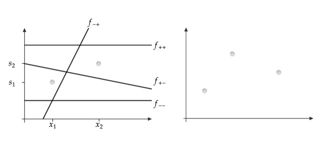
Let be a class of real-valued functions with domain . Let , and consider a collection of reals . When evaluated at each , a function will lie on one side222We adopt the notation of for well-definedness, but the other option is equally valid. of the corresponding , i.e. . The vector of such sides is thus an element of .
We say that P-shatters if there exist reals such that all possible sign combinations are obtained, i.e.,
The pseudo-dimension is the cardinality of the largest set that is P-shattered:
| (1) |
We note that the classical definition of the VC dimension takes a similar form, but without the biases and with being a class of binary functions taking values in . The pseudo-dimension satisfies similar properties as the VC dimension, such as coinciding with the standard notion of dimension for vector spaces of functions.
Proposition 2.2 (Anthony & Bartlett 1999, Thm. 11.4).
If is an -vector space of real-valued functions, then as a vector space. In particular, if is a subset of a vector space of real-valued functions, then .
Much like the VC dimension and other statistical complexity quantities such as Rademacher complexity or Gaussian complexity, low complexity leads to better generalization properties of empirical risk minimizers (Bartlett & Mendelson, 2002). One example is as follows, where precise definitions can be found in Appendix A. Informally, the -sample complexity measures the generalization performance of an approximate empirical risk minimizer, given by the number of samples such that an approximate empirical risk minimizer has true risk at most above the optimum with probability .
Proposition 2.3 (Anthony & Bartlett 1999, Thm. 19.2).
Let be a class of functions mapping from a domain into , and that has finite pseudo-dimension. Then the -sample complexity is bounded by
| (2) |
To compare the approximation of one function class by another, we consider a nonlinear width induced by a normed space.
Definition 2.4.
Let be a normed space of functions. Given two subsets , the (asymmetric) Hausdorff distance between the two subsets is the largest distance of an element of to its closest element in :
| (3) |
For a subset , the nonlinear -width is given by the optimal (asymmetric) Hausdorff distance between and , infimized over classes in with :
| (4) |
This width measures the complexity in terms of how closely the entire function class can be approximated with another class of finite pseudo-dimension. In Section 3, we provide a lower bound on the nonlinear -width of a bounded Sobolev class of functions. In terms of neural network approximation, these lower bounds complement existing approximation results of ReLU networks, which effectively provide an upper bound on the width by using the class of (bounded width, layers and parameters) ReLU networks as the finite pseudo-dimension approximating class.
2.2 Riemannian Geometry
We begin with some basic definitions, as well as recall the Bishop-Gromov comparison theorem, a volume argument that will be used throughout the next section. We give informal definitions of the sectional and Ricci curvature, and refer to Bishop & Crittenden (2011); Gallot et al. (2004) for a more detailed exposition.
Definition 2.5.
A -dimensional Riemannian manifold is a real smooth manifold equipped with a Riemannian metric , which defines an inner product on the tangent plane at each point . We assume is smooth, i.e. for any smooth chart on , the components are .
A manifold is without boundary if every point has a neighborhood homeomorphic to an open subset of .
The sectional (or Riemannian) curvature takes at each point , a tangent plane and outputs a scalar value. The Ricci curvature of a unit vector is the mean sectional curvature over planes containing a given unit vector in . The scalar curvature is the trace of the Ricci curvature.
The injectivity radius at a point is the supremum over radii such that the exponential map defines a global diffeomorphism (nonsingular derivative) from onto its image in . The injectivity radius of a manifold is the infimum of such injectivity radii over all points in .
A Riemannian manifold has a (unique) natural volume form, denoted . In local coordinates, the volume form is
| (5) |
where is the Riemannian metric, and is a (positively-oriented) cotangent basis.
Out of the three concepts of curvature, the sectional curvature is the most descriptive, and a complete understanding of the sectional curvature gives Riemannian geometry. In particular, for a manifold with constant sectional curvature , we have and .
Intuitively, the Ricci curvature controls the behavior of geodesics that are close. For manifolds of positive Ricci curvature, such as on a sphere, geodesics tend to converge. In manifolds with negative Ricci curvature, such as hyperbolic space, geodesics tend to diverge.
Within the ball of injectivity, geodesics are minimizing curves. The injectivity radius defines the largest ball on which the geodesic normal coordinates may be used, where it locally behaves as . This is an intrinsic quantity of the manifold, which does not depend on the embedding.
The volume form can be thought of as a higher-dimensional surface area, where the scaling term arises from curvature and choice of coordinates. For example, for the 2-sphere embedded in , the volume form is simply the surface measure, which can be expressed in terms of polar coordinates. We drop the subscripts when taking the volume of the whole manifold .
Throughout, we will assume that our Riemannian manifold is complete, compact, without boundary, and connected. We note that the connectedness assumption can be dropped by working instead on each connected component, since the arguments will be intrinsic and do not depend on any embeddings. We briefly state some properties of compact Riemannian manifolds.
Proposition 2.6.
Let be a compact Riemannian manifold without boundary. The following statements hold.
-
1.
(Bounded curvature) The sectional curvature (and hence the Ricci curvature) is uniformly bounded from above and below (Bishop & Crittenden, 2011, Sec. 9.3).
-
2.
(Positive injectivity radius) Let the sectional curvature be bounded by some . Suppose there exists a point and constant such that . Then there exists a positive constant such that (Cheeger et al., 1982; Grant, ):
In particular, since is compact, using a finite covering argument, is bounded below by some positive constant.
We now state the celebrated Bishop-Gromov theorem (Petersen, 2006; Bishop, 1964). This is an essential volume-comparison theorem.
Theorem 2.7 (Bishop-Gromov).
Let be a complete -dimensional Riemannian manifold whose Ricci curvature is bounded below by , for some . Let be the complete -dimensional simply connected space of constant sectional curvature , i.e. a -sphere of radius , -dimensional Euclidean space, or scaled hyperbolic space if , , respectively. Then for any and , we have that
| (6) |
is non-increasing on . In particular, .
A simple corollary that uses the volume of a hyperbolic ball to specify the rate of change in closed form is given as follows (Block et al., 2020; Ohta, 2014). We write for to mean that holds for all unit vectors in the tangent bundle .
Corollary 2.8.
Let be a -dimensional Riemannian manifold such that for some . For any point , let be the metric ball around in with radius . For any , we have
| (7) |
2.3 Sobolev Functions on Manifolds
Equipped with curvature results on the manifold, we need to define the desired function class that we wish to bound. We define Sobolev spaces in a relatively informal manner, and restrict the exposition to compact Riemannian manifolds. Note that there are many different ways to define the Sobolev spaces on manifolds due to the curvature, and we consider the variant presented in Hebey (2000).
Definition 2.9 (Hebey 2000, Sec. 2.2).
Let be a smooth Riemannian manifold. For integer , , and smooth , define by the ’th covariant derivative of , and the norm, defined in a local chart333Recall that in a chart , . as
| (8) |
using Einstein’s summation convention where repeated indices are summed. Define the set of admissible test functions (with respect to the volume measure) as
| (9) |
and for , the Sobolev norm
| (10) |
The Sobolev spaces are defined as follows, where is a -multi-index:
| (11) | ||||
It can be shown that Sobolev functions on a compact Riemannian manifold share similar embedding properties as in Euclidean space. Moreover, the weak Sobolev space is the same as , the completion of all functions with -integrable derivatives up to order with respect to the Sobolev norm (Adams & Fournier, 2003; Meyers & Serrin, 1964). We briefly mention the manifold versions of the embedding theorems and Morrey’s inequality, which embed into spaces and Hölder spaces respectively. Other corresponding inclusions such as Rellich-Kondrachov and Sobolev-Poincaré also continue to hold, and we refer to Hebey (2000) for a more detailed treatment.
We adopt the following definition of a bounded Sobolev ball. This is a natural extension of a -ball to Sobolev spaces and provides a compact space of functions to approximate.
Definition 2.10.
For constant , the bounded Sobolev ball is given by the set of all functions with weak derivatives bounded in by :
| (12) |
We write to mean for ease of notation.
We note that it is possible to have other definitions of bounded Sobolev functions, such as bounding only the -norm of one multi-indexed derivative. However, this will only change the bounds up to some constant. In the following section, we derive a lower bound on the nonlinear -width of bounded Sobolev balls in .
3 Main Result
This section begins with a statement of the main approximation result, followed by high-level intuition behind the proof. We then state several lemmas that will be useful, and finish with the proof.
3.1 Statement
Theorem 3.1.
Let be a -dimensional compact (separable) Riemannian manifold without boundary. From compactness, there exist real constants such that:
-
1.
The Ricci curvature satisfies , where ;
-
2.
is the injectivity radius;
Moreover, for any , the nonlinear width of satisfies the lower bound for sufficiently large :
| (13) |
In particular, the constant is independent of any latent dimension that may be embedded in.
We note that since the manifold Sobolev space is defined directly on the manifold, embeddings are not necessary, which removes any dependence on latent dimension. This theorem should be contrasted with Maiorov & Ratsaby (1999, Thm. 1), which produces a similar bound for the bounded Sobolev space on , but with lower bound . The additional term is necessary due to the curvature of the space. We also note that it is possible to perform this analysis in the case of positive curvature.
There are two major differences in converting the proof of Maiorov & Ratsaby (1999) to the manifold setting. Firstly, Maiorov & Ratsaby (1999) uses a partition into hypercubes to construct the desired counterexample. As such hypercube partitions generally do not pose nice properties on manifolds, this must be loosened to a packing of geodesic balls, which does not fully cover the manifold and loosens the bound. The second major difference is the presence of curvature and its non-locality, where geodesic balls of the same radius can have drastically different volumes, even if it is pointwise asymptotically Euclidean. This will introduce additional constants into the final bound.
3.2 Proof Sketch
The proof follows a the ideas for a similar statement in Maiorov & Ratsaby (1999) for the cube , with slight corrections and explicit constant tracking. The major differences arise due to the curvature, where small-ball volumes are pointwise asymptotically Euclidean, but not uniformly over the entire manifold. We can break down the proof into several steps.
-
Step 1.
We consider a class of simple functions, defined as sums of cutoff functions with disjoint supports. The class of simple functions is such that the -norm of each component is large within the class of bounded functions.
-
Step 2.
An appropriate subset of the simple functions is then taken, that is isometric to the -hypercube. Since the vertices of the hypercube are -well separated, there exists an -well-separated subset of our class of functions.
-
Step 3.
We then show that it is not possible to bypass the given bound by trying to approximate the constructed set of well-separated functions with a low-pseudodimension class. This step uses an exponential lower bound on the metric entropy and a polynomial upper bound from Bishop-Gromov to derive a contradiction.
3.2.1 Packing Lemmas
We list a few lemmas that will be useful. Proofs are given in Appendix B for completeness. We use the following definition of covering number.
Definition 3.2 (Covering number).
For a metric space and radius , the covering number is the maximum number of points such that the open balls are disjoint. The metric entropy is the maximum number of points such that for .
Remark 3.3.
The following inequality holds:
| (14) |
The first inequality holds since any -separated subset has disjoint -balls. The second inequality holds since any set with disjoint -balls is necessarily -separated.
Proposition 3.4 (Packing number estimates).
Suppose has curvature lower-bounded by , diameter and dimension . Let be the -dimensional model space of constant sectional curvature (i.e. sphere, Euclidean space, or hyperbolic space). The packing number satisfies, where is any point in :
| (15) |
Proof.
Uses Bishop-Gromov. Deferred to Proposition B.1. ∎
We note that the volume of a ball of given radius in space of constant curvature is independent of the given point. We drop the where necessary, and write
to denote the volume of any ball of radius in . We finish the required expositions with a bound on the metric entropy for bounded functions.
Lemma 3.5 (Haussler 1995, Cor. 2 and 3).
For any set , any probability distribution on , any distribution on , any set of -measurable real-valued functions on with and any , the metric entropy (largest cardinality of a -separated subset, where distance between any two elements is ) satisfies:
| (16) |
Specifically, taking distance, if is -measurable taking values in the interval , we have
| (17) |
If is instead a finite measure, and is -measurable taking values in the interval , then
| (18) |
Remark 3.6.
The final inequality comes from the second-to-last inequality, by noting that a -separated set in corresponds to a -separated set in the normalized measure , as well as scaling everything by .
3.3 Proof
We now continue with the proof of Theorem 3.1. In the following, spaces will be on with respect to the underlying volume measure. Recall the definition of the bounded class of functions:
| (19) |
Step 1. Defining the base function class. Fix a radius , which will be chosen appropriately later. Consider a maximal packing of geodesic -balls, say with centers , where is the packing number. By definition, are disjoint for . From Proposition 3.4 the packing number satisfies
| (20) |
For each ball , we can construct a function with support such that
| (21) |
This can be done by constructing a cutoff function and finding an appropriate smooth approximation for separable Riemannian manifolds, using infimal convolutions and partitions of unity (Azagra et al., 2007, Cor. 3). In particular, we can choose to have pointwise. From 21, we have the lower bound
| (22) |
Moreover, we have the bounds on and
| (23) | |||
| (24) |
Therefore, for , we have that . Defining
| (25) |
we get a non-negative function with support in satisfying:
| (26) |
Moreover, on . We now consider the function class
| (27) |
Since the sum is over functions of disjoint support, we have that , and thus each element of also lies in . Moreover, every element satisfies the lower bound using 26:
| (28) |
Step 2. -well-separation of . Consider the following lemma, which shows existence of a large well-separated subset of .
Lemma 3.7 (Lorentz et al. 1996, Lem. 2.2).
There exists a set of cardinality at least such that for any , the distance . In particular, any two elements differ by at least entries.
In particular, let be well separated by the above lemma. Denote by the subset of corresponding to these indices:
| (29) |
For the specific choice of separated in the above lemma, we claim the following well-separation.
Claim 1.
There exists constant such that for any , we have
| (30) |
Proof.
Suppose . In particular, they are generated by multi-indices . Consider the set of indices such that . By construction in Lemma 3.7, . Then the difference between and on is if , and 0 otherwise. By disjointness of the , we have
| (31) | ||||
| (32) | ||||
| (33) | ||||
| (34) |
by the -bound on , Bishop-Gromov (Corollary 2.8), and using for the inequalities respectively. ∎
This shows -well separation of the subset , which consist of sums of disjoint cutoff functions. The key will now be to contrast this with the metric entropy bounds in Lemma 3.5, by showing that is difficult to approximate with low pseudo-dimension function classes.
Step 3a. Construction of well-separated bounded set. Let be a given set of -measurable functions with . Let . Denote
| (35) |
Define a projection operator , mapping any to any element in such that
| (36) |
We introduce the clamping operator for a function :
| (37) | |||
| (38) |
Note that are the bounds of in the balls . Now consider the set of functions . Suppose . We show separation in :
| (39) |
For any , we have that in , and both and are zero on . We thus have that for any and any ,
| (40) |
This inequality holds for since clamps towards , and holds trivially . Integrating and using 36, we have that for any ,
| (41) |
Using 39, 41 and 34, we thus have separation
| (42) | ||||
| (43) |
For ease of notation, define the -separation distance to be :
| (44) |
Step 3b. Minimum distance by contradiction. Suppose for contradiction that . Then from 42, we have
| (45) |
In particular, the separation implies that the are distinct for distinct , thus .
Define . Consider the metric entropy in , as given in Lemma 3.5. By construction 42, itself is an -separated subset in as any two elements are -separated by , so
| (46) |
We now wish to obtain an upper bound on using Lemma 3.5. From the definition of pseudo-dimension, we have , since any P-shattering set for will certainly P-shatter . Since , we have . Thus . is -separated with distance at least , and moreover consists of elements that are bounded by . We can now use 18 in Lemma 3.5 to obtain:
| (47) |
Intuitively, , so the lower bound 46 is exponential in . Meanwhile, and are both polynomial in , so the upper bound 47 is polynomial in . So for sufficiently small , we have a contradiction, which gives a lower bound on . We now show this formally. Recall:
| (48) |
Note that the supremum in and the infimum in is attained by the same , namely, the that has smallest .444Intuitively, tall thin functions have the worst to ratio compared to short fat functions. By construction, small balls have tall thin functions. Combining 46 and 47, where ,
| (49) |
where the equalities come from definition of and and rearranging, and the last equality from noting the supremum is attained when minimizes . Recall from 20 that
| (50) |
Proposition 3.8 (Croke 1980, Prop. 14).
For , the volume of the ball satisfies
| (51) |
We note that a closed-form for the volume of a -dimensional ball is given as
| (52) |
where is Euler’s gamma function satisfying if is a positive integer and if is a non-negative integer. Moreover, the volume of the -dimensional hyperbolic sphere with sectional curvature is
| (53) |
Note that for . Therefore, for , we have . We thus have that
| (54) |
where
| (55) |
We continue the inequality 49 for :
We note that
| (60) |
since for . We thus have for , that
| (61) |
where
| (62) |
We get a contradiction if
| (63) |
Recalling the lower bound 20 on and using 60,
| (64) |
Take the following choice of :
| (65) |
Using 64, this choice of satisfies the contradiction condition 63. Note . The constants depend only on .
Step 4. Concluding contradiction. This choice of contradicts the assumption that . Therefore, we must have that . Since the choice of is independent of the choice of taken at the start of Step 3a, we have that
| (66) |
where is chosen as in 65. We obtain the chain of inequalities
| (67) |
where the first inequality comes from Hölder’s inequality , the second inequality from , the third from 66 and the equality from definition 44 of .
We conclude with recalling the bounds 60, 64, and Proposition 3.8. Together we have
The constant is
| (68) |
Moreover, the constant and choice of are independent of . Taking infimum over all choice of with and using 65, we have
| (69) |
4 Conclusion
This work provides a theoretical motivation to further explore the manifold hypothesis. We show that the problem of approximating a bounded class of Sobolev functions depends only on the intrinsic properties of the space it is supported in. More precisely, the approximation error of the bounded space with respect to bounded pseudo-dimension classes is shown to be at least , where is the intrinsic dimension of the underlying manifold. Since generalization error is linear in pseudo-dimension, this provides a latent-dimension-free lower-bound on generalization error. This is in contrast to many works in the literature that provide constructive upper bounds on generalization error based on ReLU approximation properties that still depend on the embedding of the manifold in latent Euclidean space.
The proposed bound can be improved in multiple ways. Firstly, the analysis is restricted to one weak derivative. The analogous result of approximating in the cube has lower bounds (Maiorov & Ratsaby, 1999). Extending our analysis to more weak derivatives would require a careful construction in Step 1 of test functions with the appropriate regularity conditions. In particular, we would require cutoff functions with explicitly bounded higher weak derivatives , which do not seem to appear in the literature. The explicit construction of Moulis (1971) of a function that approximates a function in the -topology could be useful in this. Moreover, the current bound requires knowledge of the injectivity radius to uniformly lower-bound the volume of small balls. Other ways of constructing volume lower-bounds would help in improving the constants in the bound.
References
- Adams & Fournier (2003) Robert A Adams and John JF Fournier. Sobolev spaces. Elsevier, 2003.
- Altman & Krzywinski (2018) Naomi Altman and Martin Krzywinski. The curse (s) of dimensionality. Nat Methods, 15(6):399–400, 2018.
- Andrychowicz et al. (2016) Marcin Andrychowicz, Misha Denil, Sergio Gomez, Matthew W Hoffman, David Pfau, Tom Schaul, Brendan Shillingford, and Nando De Freitas. Learning to learn by gradient descent by gradient descent. Advances in neural information processing systems, 29, 2016.
- Anthony & Bartlett (1999) Martin Anthony and Peter L. Bartlett. Neural network learning: Theoretical foundations, volume 9. Cambridge university press, 1999.
- Azagra et al. (2007) Daniel Azagra, Juan Ferrera, Fernando López-Mesas, and Yenny Rangel. Smooth approximation of Lipschitz functions on Riemannian manifolds. Journal of Mathematical Analysis and Applications, 326(2):1370–1378, 2007.
- Bartlett & Mendelson (2002) Peter L Bartlett and Shahar Mendelson. Rademacher and Gaussian complexities: Risk bounds and structural results. Journal of Machine Learning Research, 3(Nov):463–482, 2002.
- Belkin & Niyogi (2001) Mikhail Belkin and Partha Niyogi. Laplacian eigenmaps and spectral techniques for embedding and clustering. Advances in neural information processing systems, 14, 2001.
- Bengio et al. (2013) Yoshua Bengio, Aaron Courville, and Pascal Vincent. Representation learning: A review and new perspectives. IEEE transactions on pattern analysis and machine intelligence, 35(8):1798–1828, 2013.
- Bishop (1964) Richard L Bishop. A relation between volume, mean curvature and diameter. In Euclidean Quantum Gravity, pp. 161–161. World Scientific, 1964.
- Bishop & Crittenden (2011) Richard L Bishop and Richard J Crittenden. Geometry of Manifolds: Geometry of Manifolds. Academic press, 2011.
- Block et al. (2020) Adam Block, Youssef Mroueh, Alexander Rakhlin, and Jerret Ross. Fast mixing of multi-scale Langevin dynamics under the manifold hypothesis. arXiv preprint arXiv:2006.11166, 2020.
- Block et al. (2021) Adam Block, Zeyu Jia, Yury Polyanskiy, and Alexander Rakhlin. Intrinsic dimension estimation using wasserstein distances. arXiv preprint arXiv:2106.04018, 2021.
- Brown et al. (2022) Bradley CA Brown, Anthony L Caterini, Brendan Leigh Ross, Jesse C Cresswell, and Gabriel Loaiza-Ganem. Verifying the union of manifolds hypothesis for image data. In The Eleventh International Conference on Learning Representations, 2022.
- Bubeck & Sellke (2021) Sébastien Bubeck and Mark Sellke. A universal law of robustness via isoperimetry. Advances in Neural Information Processing Systems, 34:28811–28822, 2021.
- Celledoni et al. (2021) Elena Celledoni, Matthias J Ehrhardt, Christian Etmann, Robert I McLachlan, Brynjulf Owren, C-B Schonlieb, and Ferdia Sherry. Structure-preserving deep learning. European journal of applied mathematics, 32(5):888–936, 2021.
- Cheeger et al. (1982) Jeff Cheeger, Mikhail Gromov, and Michael Taylor. Finite propagation speed, kernel estimates for functions of the laplace operator, and the geometry of complete riemannian manifolds. Journal of Differential Geometry, 17(1):15–53, 1982.
- Chen et al. (2021) Dongdong Chen, Julián Tachella, and Mike E Davies. Equivariant imaging: Learning beyond the range space. In Proceedings of the IEEE/CVF International Conference on Computer Vision, pp. 4379–4388, 2021.
- Chen et al. (2019) Minshuo Chen, Haoming Jiang, Wenjing Liao, and Tuo Zhao. Efficient approximation of deep relu networks for functions on low dimensional manifolds. Advances in neural information processing systems, 32, 2019.
- Chen et al. (2022) Minshuo Chen, Haoming Jiang, Wenjing Liao, and Tuo Zhao. Nonparametric regression on low-dimensional manifolds using deep relu networks: Function approximation and statistical recovery. Information and Inference: A Journal of the IMA, 11(4):1203–1253, 2022.
- Cohen & Welling (2016) Taco Cohen and Max Welling. Group equivariant convolutional networks. In International conference on machine learning, pp. 2990–2999. PMLR, 2016.
- Connor et al. (2021) Marissa Connor, Gregory Canal, and Christopher Rozell. Variational autoencoder with learned latent structure. In International conference on artificial intelligence and statistics, pp. 2359–2367. PMLR, 2021.
- Croke (1980) Christopher B Croke. Some isoperimetric inequalities and eigenvalue estimates. In Annales scientifiques de l’École normale supérieure, volume 13, pp. 419–435, 1980.
- DeMers & Cottrell (1992) David DeMers and Garrison Cottrell. Non-linear dimensionality reduction. Advances in neural information processing systems, 5, 1992.
- Fefferman et al. (2016) Charles Fefferman, Sanjoy Mitter, and Hariharan Narayanan. Testing the manifold hypothesis. Journal of the American Mathematical Society, 29(4):983–1049, 2016.
- Gallot et al. (2004) Sylvestre Gallot, Dominique Hulin, Jacques Lafontaine, et al. Riemannian geometry, volume 3. Springer, 2004.
- Gao et al. (2019) Ruiqi Gao, Tianle Cai, Haochuan Li, Cho-Jui Hsieh, Liwei Wang, and Jason D Lee. Convergence of adversarial training in overparametrized neural networks. Advances in Neural Information Processing Systems, 32, 2019.
- (27) James D.E. Grant. Injectivity radius estimates i. URL https://homepage.univie.ac.at/james.grant/papers/NullInj/Inj_rad_talk_1.pdf. Accessed July 12th, 2024.
- Haussler (1995) David Haussler. Sphere packing numbers for subsets of the Boolean n-cube with bounded Vapnik-Chervonenkis dimension. Journal of Combinatorial Theory, Series A, 69(2):217–232, 1995.
- Hebey (2000) Emmanuel Hebey. Nonlinear analysis on manifolds: Sobolev spaces and inequalities: Sobolev spaces and inequalities, volume 5. American Mathematical Soc., 2000.
- Kamilov et al. (2023) Ulugbek S Kamilov, Charles A Bouman, Gregery T Buzzard, and Brendt Wohlberg. Plug-and-play methods for integrating physical and learned models in computational imaging: Theory, algorithms, and applications. IEEE Signal Processing Magazine, 40(1):85–97, 2023.
- Kingma & Welling (2013) Diederik P Kingma and Max Welling. Auto-encoding variational bayes. arXiv preprint arXiv:1312.6114, 2013.
- Labate & Shi (2023) Demetrio Labate and Ji Shi. Low dimensional approximation and generalization of multivariate functions on smooth manifolds using deep neural networks. Available at SSRN 4545106, 2023.
- Lee et al. (2007) John A Lee, Michel Verleysen, et al. Nonlinear dimensionality reduction, volume 1. Springer, 2007.
- Levina & Bickel (2004) Elizaveta Levina and Peter Bickel. Maximum likelihood estimation of intrinsic dimension. Advances in neural information processing systems, 17, 2004.
- Lorentz et al. (1996) George G Lorentz, Manfred von Golitschek, and Yuly Makovoz. Constructive approximation: advanced problems, volume 304. Citeseer, 1996.
- Maiorov & Ratsaby (1999) Vitaly Maiorov and Joel Ratsaby. On the degree of approximation by manifolds of finite pseudo-dimension. Constructive approximation, 15(2):291–300, 1999.
- Meyers & Serrin (1964) Norman Meyers and James Serrin. H = w. Proceedings of the National Academy of Sciences of the United States of America, 51 6:1055–6, 1964.
- Moulis (1971) Nicole Moulis. Approximation de fonctions différentiables sur certains espaces de Banach. In Annales de l’institut Fourier, volume 21, pp. 293–345, 1971.
- Nakada & Imaizumi (2020) Ryumei Nakada and Masaaki Imaizumi. Adaptive approximation and generalization of deep neural network with intrinsic dimensionality. Journal of Machine Learning Research, 21(174):1–38, 2020.
- Narayanan & Niyogi (2009) Hariharan Narayanan and Partha Niyogi. On the sample complexity of learning smooth cuts on a manifold. In COLT, 2009.
- Niyogi et al. (2008) Partha Niyogi, Stephen Smale, and Shmuel Weinberger. Finding the homology of submanifolds with high confidence from random samples. Discrete & Computational Geometry, 39:419–441, 2008.
- Niyogi et al. (2011) Partha Niyogi, Stephen Smale, and Shmuel Weinberger. A topological view of unsupervised learning from noisy data. SIAM Journal on Computing, 40(3):646–663, 2011.
- Ohta (2014) Shin-Ichi Ohta. Ricci curvature, entropy, and optimal transport, pp. 145–200. London Mathematical Society Lecture Note Series. Cambridge University Press, 2014.
- Petersen (2006) Peter Petersen. Riemannian geometry, volume 171. Springer, 2006.
- Pollard (2012) David Pollard. Convergence of stochastic processes. Springer Science & Business Media, 2012.
- Pope et al. (2021) Phillip Pope, Chen Zhu, Ahmed Abdelkader, Micah Goldblum, and Tom Goldstein. The intrinsic dimension of images and its impact on learning. arXiv preprint arXiv:2104.08894, 2021.
- Roweis & Saul (2000) Sam T Roweis and Lawrence K Saul. Nonlinear dimensionality reduction by locally linear embedding. science, 290(5500):2323–2326, 2000.
- Shwartz-Ziv & Tishby (2017) Ravid Shwartz-Ziv and Naftali Tishby. Opening the black box of deep neural networks via information. arXiv preprint arXiv:1703.00810, 2017.
- Tan et al. (2023) Hong Ye Tan, Subhadip Mukherjee, Junqi Tang, and Carola-Bibiane Schönlieb. Data-driven mirror descent with input-convex neural networks. SIAM Journal on Mathematics of Data Science, 5(2):558–587, 2023.
- Tenenbaum et al. (2000) Joshua B Tenenbaum, Vin de Silva, and John C Langford. A global geometric framework for nonlinear dimensionality reduction. science, 290(5500):2319–2323, 2000.
- Tishby & Zaslavsky (2015) Naftali Tishby and Noga Zaslavsky. Deep learning and the information bottleneck principle. In 2015 ieee information theory workshop (itw), pp. 1–5. IEEE, 2015.
- Venkatakrishnan et al. (2013) Singanallur V Venkatakrishnan, Charles A Bouman, and Brendt Wohlberg. Plug-and-play priors for model based reconstruction. In 2013 IEEE global conference on signal and information processing, pp. 945–948. IEEE, 2013.
- Vidal (2011) René Vidal. Subspace clustering. IEEE Signal Processing Magazine, 28(2):52–68, 2011.
- Wainwright (2019) Martin J Wainwright. High-dimensional statistics: A non-asymptotic viewpoint, volume 48. Cambridge university press, 2019.
- Wang et al. (2020) Xiao Wang, Qi Lei, and Ioannis Panageas. Fast convergence of Langevin dynamics on manifold: Geodesics meet log-Sobolev. Advances in Neural Information Processing Systems, 33:18894–18904, 2020.
- Wang et al. (2016) Yasi Wang, Hongxun Yao, and Sicheng Zhao. Auto-encoder based dimensionality reduction. Neurocomputing, 184:232–242, 2016.
- Yang et al. (2024) Yahong Yang, Haizhao Yang, and Yang Xiang. Nearly optimal vc-dimension and pseudo-dimension bounds for deep neural network derivatives. Advances in Neural Information Processing Systems, 36, 2024.
Appendix A Sample complexity
For completeness, we briefly formalize the sample complexity bound Proposition 2.3, based on (Anthony & Bartlett, 1999).
Definition A.1 (Anthony & Bartlett 1999, Def. 16.4).
For a set of functions , an approximate sample error minimizing (approximate-SEM) algorithm takes any finite number of samples in and an error bound , and outputs an element satisfying
| (70) |
Definition A.2 (Anthony & Bartlett 1999, Def. 16.1).
For a set of functions mapping from domain to , a learning algorithm for is a function taking any finite number of samples,
| (71) |
with the following property. For any , there is an integer such that if , the following holds for any probability distribution on .
If is a training sample of length according to the product distribution (i.i.d. samples), then with probability at least , the function output by is such that
| (72) |
In other words, given training samples, the squared-risk of the learning algorithm’s output is -optimal with probability at least .
Observe that the approximate-SEM algorithm works on the empirical risk, while the learning algorithm works on the risk. Relating the two thus gives generalization bounds. The formal version of Proposition 2.3, based on (Anthony & Bartlett, 1999) is now given as follows.
Proposition A.3 (Anthony & Bartlett 1999, Thm. 19.2).
Let be a class of functions mapping from a domain into , and that has finite pseudo-dimension. Let be any approximate-SEM algorithm, and define for samples , . Then is a learning algorithm for , and its sample complexity is bounded as follows:
| (73) |
Appendix B Proof of lemmas.
Proposition B.1 (Covering number estimates).
Suppose has curvature lower-bounded by , diameter and dimension . Let be the -dimensional model space of curvature (i.e. sphere, Euclidean space, or hyperbolic space). The packing number satisfies:
| (74) |
Proof.
Let be an -packing of .
Lower bound. By maximality, balls of radius at the cover , so we have by summing over volumes and using Bishop-Gromov:
| (75) |
Upper bound. Apply Theorem 2.7 with . We have . Since the -balls are disjoint, we have by finite additivity and Bishop-Gromov:
| (76) |
∎