Kink-antikink collisions in hyper-massive models
Abstract
We study topological kinks and their interactions in a family of scalar field models with a double well potential parametrized by the mass of small perturbations around the vacua, ranging from the mass of the Klein-Gordon model all the way to the limit of infinite mass, which is identified with a non-analytic potential. In particular, we look at the problem of kink-antikink collisions and analyze the windows of capture and escape of the soliton pair as a function of collision velocity and model mass. We observe a disappearance of the capture cases for intermediary masses between the and non-analytic cases. The main features of the kink-antikink scattering are reproduced in a collective coordinates model, including the disappearance of the capture cases.
I Introduction
Classical solutions of scalar fields are interesting due to their applications in a wide range of physical phenomena, from condensed matter systems to large cosmological settings. Topological defect solutions, also known as topological solitons, are specially significant due to their applications and intricate dynamics [1]. In the dimensional case, the sine-Gordon model and the Klein-Gordon model are classical examples of theories supporting topological defects known as kinks. The interaction of topological kinks in those and other models has been an active topic of research for over four decades, with many fascinating phenomena still to be explained [2]. The sine-Gordon model is remarkable for being an integrable model, allowing its kinks to collide elastically. Meanwhile, the model has inelastic collisions featuring resonances cases, where a kink-antikink pair annihilates, oscillates a few times, and then escapes. Recently, the resonance windows, among other features of kink-antikink interaction, have been better understood using a moduli space approach [3, 4, 5, 6, 7, 8, 9].
Topological defects, like the kinks in the theory, are usually infinite in size, i.e. the field reaches the vacuum values only asymptotically through an exponential tail , where is the field mass and is the distance. A fascinating exception is the case of compactons: solutions contained in a compact support, reaching the vacuum at a finite distance. Compactons were first discovered for a modified Korteweg–De Vries (KdV) equation [10], but have since also been found in relativistic models with non-differentiable potential at its minima.
Potentials that are non-differentiable at the minima, also known as non-analytic or V-shaped potentials, were first discussed in the continuum limit of mechanical models where the motion is limited by rigid barriers [11]. Since then, it was shown that in certain cases the first Bogomol’nyi-Prasad-Sommerfield (BPS) submodel of the Skyrme model [12], is equivalent to a scalar field theory with a non-analytic periodic potential [13]. The collision of compact kinks in such model was recently studied [14]. It was shown that, at least for that model, the compact kink-antikink scattering does not have resonance cases and that the transition from the cases of capture to the cases of escape of the soliton pair has a fractal nature. In the case of compactons, the distinct mathematical nature of those solutions constrains the construction of the kink-antikink moduli space, making the determination of internal models that may contribute to the scattering moduli space more nuanced.
In this paper, we approach the problem of topological compacton interactions from a different perspective, building on a previous result that a non-analytic potential with compact solutions can be obtained by continually deforming the potential function [15]. The parameter of the deformation is related to the mass of small perturbations around the model vacua in such a way that the non-analytic model corresponds to the limit of infinite mass. The identification of non-analytic potentials with infinitely massive fields has also been made in the case of a single well potential [16]. In this sense, we can say that non-analytic models correspond to the hyper-massive limit of more usual models. By studying how the features of kink-antikink scattering change during the transition from the to a non-analytic model, we seek to deepen the understanding of the unique features of compactons and their interactions.
In this paper, we improve on our previous results on compacton scattering by using kink internal modes derived from first principles instead of phenomenological arguments. Furthermore, the model in the present paper has a more traditional double well potential, while the potential in our previous works was periodic. This allows for a more objective verification of which results are actually due to non-analytic nature of the potential. We also show that the transition from the model to non-analytic models is not as straightforward as it appears. In some senses, we found that the interaction of kinks in the and in the hyper-massive model have more in common with one another than with intermediary cases.
This paper is organized as follows. In section II we present the model studied, reviewing some of its properties and the properties of the kink solution. We also solve for the first kink internal mode for all values of the potential parameter. In section III we discuss the moduli space of a single kink, including its Derrick mode and its similarity with the first kink internal mode. We present simulation results for kink-antikink collisions in section IV, with special attention to the identification of cases of capture or escape of the soliton pair. Some simulation results are explained through the moduli space approach in section V. We summarize our conclusions in section VI.
II Model
We consider a model for a scalar field in dimensions defined by the Lagrangian density
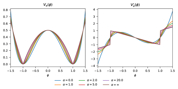
where is a double well potential with minima at . The potential is the one defined in ref. [15], given explicitly by
where the parameter is a real positive number. The limiting cases for the parameter correspond to the potential of the Klein-Gordon model and an analogous non-analytic model:
For simplicity, every time we talk about the cases and we leave implied the procedure of taking the limit and simply say that or .
The field dynamics is determined by the Euler-Lagrange equation
where is the potential derivative with the expression
Its limiting cases are
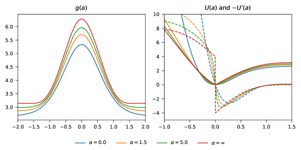
Note that is discontinuous at the potential minima, which is a defining characteristic of non-analytic potentials, allowing for the existence of compact solutions. Also, we must impose that so that the vacuum configurations are solutions to the Euler-Lagrange equations. This also agrees with the definition of derivative in the distributional sense. Examples of the potential and its derivative for different values of are shown in figure 1.
Small field perturbations around the two vacua have squared mass equal to the second derivative of the potential:
Therefore, we can alternatively parametrize the potential by the field mass:
The usual potential can be recovered by taking the limit while the non-analytic case can be recovered in the limit . In this sense, we say that models with non-analytic potential are a hyper-massive limit. Note that this mass is expressed in dimensionless units, and can not be rescaled away. It is an unavoidable parameter of the potential, which influences its shape beyond simple scale transformations.
There is yet another useful parametrization using the variable
The parameter is useful when exploring the transition to the non-analytic case. Since the range of is limited the non-analytic case can be reached by taking the limit from the left, a case we refer simply as the case. The potential in terms of is:
The corresponding mass parameter takes the form .
Since the potential is degenerate for all values of the parameter , topological kink solutions can be found by integrating the BPS equation
| (1) |
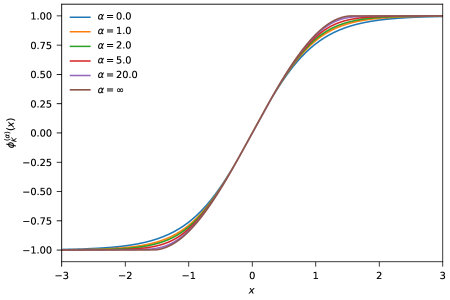
with appropriate boundary conditions. For we get the usual kink
while for we get the compact kink solution
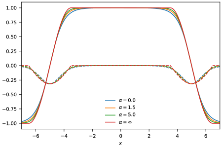
For other values of , the kink solution does not have an analytical expression, but it can be found by numerically integrating equation (1). Some examples are presented in figure 2. Due to the symmetry of the model, antikink solutions are simply . Note that the potential for the region between the two minima, i.e. , has the same shape that of the periodic potential of refs. [13, 17, 14]. Therefore, the compact kink has the same profile shape as the one in those works.
These kink and antikink solutions are static, however moving kink solutions with velocity can be found by exploring the Lorentz symmetry of the model, such that a moving kink solution is given by
where .
Another possibility for dynamical behavior is to have the kink internal modes to be excited. We can find the kink internal modes by writing the field as a kink profile with a small oscillating perturbation in the form
| (2) |
where is the internal mode angular frequency, and we temporally stopped writing the dependency in for simplicity. Plugging this expression on the field equation
and assuming the perturbation is small, we obtain
which leads to the following Schrödinger-like equation for the perturbation
| (3) |
In general, the first eigenvalue is zero and corresponds to the translational mode of the kink. The second eigenvalue gives the frequency square of the first internal mode. For the case , this is the well-known shape mode with frequency . The shape mode of the kink is very widely studied, therefore we will not discuss it in detail.
We can also get closed form expressions for the internal modes of the non-analytic potential in the hyper-massive limit. The function acts as the potential function for this equation. For the non-analytic potential
This function has divergent derivative for , therefore is infinite for , because when the kink has a compact support and reaches the vacua at these points. This can also be visualized by looking the potential function for increasingly large values of , as in figure 3.
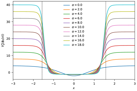
Therefore, for the compact kink internal modes we must solve equation (3) for
which is equivalent to the quantum mechanical problem of finding the wave function of a particle trapped in an infinite well. It has been shown [15] that the eigenvalues are for , which agrees with the textbook result for an infinite potential well. Surprisingly, the first mode has frequency equal to the frequency of the shape mode in the model. The eigenfunctions corresponding to each are simply trigonometric functions truncated to the kink support
Note that is simply the translational mode.
By regularizing the potential we gain a simpler approach to analyzing the translational mode. While directly perturbing the compact kink, as shown in equation (2), within the non-analytic model presents technical difficulties, such as dividing the problem into separate spatial regions, leading to patched formulas, and handling Dirac deltas function arising from the second derivative of the potential, the regularized approach offers a clearer path. Here, the emergence of a square infinite well potential becomes evident, providing a well-defined method for obtaining the perturbation modes, including the translational mode. Also note that the compacton internal mode in this work is different from the phenomenological mode used in refs. [17, 14], which was actually .
For non-zero finite values of , the eigenvalue problem can not be solved analytically. However, we can solve it numerically by discretizing the differential operator. We present the first mode and its frequency for different in figure 4. Much like the kink itself, the internal mode becomes compact in the hyper-massive limit .
III Single kink moduli space
The moduli space approach, also known as collective coordinates approximation, is an important tool in the description of kink collisions since its earliest uses in the description of kink-antikink collisions in the model [18]. In this approach, one writes a tentative expression for the field as a function of a finite number of degrees of freedom known as collective coordinates or moduli. The time dependence of the field is then completely determined by , i.e. . The Lagrangian density for the field can be integrated to obtain a classical mechanics Lagrangian for the coordinates with expression
in terms of an effective metric
| (4) |
and effective potential
| (5) |
in the space of the coordinates . Note that the metric is for the moduli space and must not be confused with the Minkowski spacetime metric. The time evolution of can be obtained by solving the Euler-Lagrange equations
| (6) |
where is the inverse of the metric tensor and are the Christoffel symbols given by
For a single kink configuration, we can explore the translational symmetry of the model to get a displaced soliton centered at with the expression , which is a solution of the field equations provided that is a constant. If we promote the kink position to a time-dependent degree of freedom, we obtain a non-relativistic moduli space with a single coordinate . It can be shown [4] that the Lagrangian for this coordinate is simply the one for a massive particle with constant potential:
where
is the kink rest energy, which is also its mass because we are using natural units.
A relativistic moduli space can be achieved by introducing an extra coordinate to account for the Lorentz contraction, so that the field has the expression
In this case, the Lagrangian can be shown [7] to have the expression
where
is the static kink second energy moment. The resulting Euler-Lagrange equations have a stationary solution , , which reproduces exactly the field equation solution of a moving kink. In the case , one can also find oscillatory solutions with frequency .
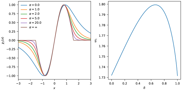
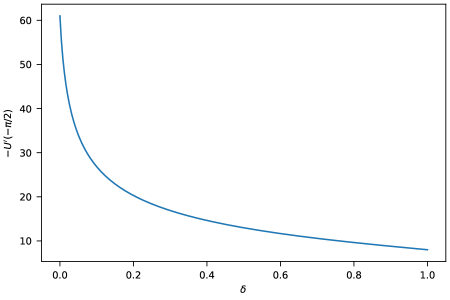
The frequency is the frequency of the Derrick mode, related to the small changes in the field caused by scale transformations of the kink solution. The profile of the Derrick mode can be obtained considering the perturbation on the kink profile by a small size deformation, i.e. close to one. In fact, for and , the field has the Taylor series
| (7) |
We identify the coefficient of first term in the series as the Derrick mode
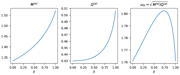
In figure 5 we present the dependency of the quantities , , and on the parameter . As the potential becomes steeper with larger the kink narrows, leading to an increase in its gradient energy reflected on the kink mass . The minimum mass, corresponds to the kink, while the maximum mass, , is for the compact kink. The antikink has a mass equal to the mass of the kink. The minimum value of the second moment is , while the maximum value is . We have
causing the Derrick mode for the cases and to have identical frequencies,
similar to what was found for the frequency of the first internal mode, .
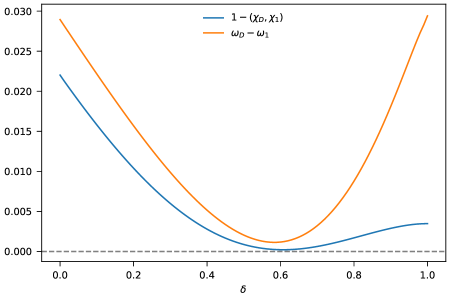
In fact, the whole curve for as function of is strikingly similar to the dependency of the first mode frequency on (figure 4). It is known that for the model the kink shape mode is very similar to the Derrick mode, both in profile and frequency. It is natural to inquire whether the observed similarity persists for all values of . To quantify the similarity between the modes, we define the inner product
between the modes. This inner product ranges from for entirely independent modes to for identical modes. Therefore, is a measure of the modes’ independence, and so is the frequencies difference . We graph the dependency of the these quantities on in figure 6. Although the two modes never become identical, they are very close for , which is also the region where and are maximum. Once again, the differences in frequency are the same for and , however, the inner product is closer to unity for the non-analytic model than in the model.
IV Kink-antikink collisions
The interaction between classical solutions offers important glimpses about the dynamics of non-linear models. The most common scenario for studying interacting configurations in models with topological kinks is the collision between a kink and an antikink. We study the problem of kink-antikink collisions in the center of momentum reference frame, where we can approximate the field initial condition by a superposition
provided that the separation is large enough for the superposition to be a good approximate solution of the field equation, i.e. for the pair to be interacting weakly. In the special case of compactons (), the functions have support of size , so the superposition correspond an exact solution of the field equation when . This initial condition contains a kink centered at moving from the left to the right with velocity , while an antikink centered at is moving from the right to the left with velocity of same absolute value, but opposite direction. Some examples of the initial condition can be seen in figure 7.
Due to the non-linear and non-integrable character of the field equations, the dynamics of a kink-antikink interaction must be obtained by numerically evolving the initial conditions. We discuss the numerical methods on the appendix. We treat and as parameters on which the simulation depends on, while fixing . Some examples of simulations for selected values of and are presented as color maps on a spacetime diagram in figure 8. In general, all initial conditions initially evolve to the annihilation of the kink-antikink pair leading to a configuration where the field bounces between the vacuum values. However, there are two broadly distinct outputs: either the field bounces indefinitely, a scenario we call capture, or the field bounces one or more times and then a kink-antikink pair emerges from the configuration and separates, a scenario we call escape. In general, the capture case correspond to small velocities , while the escape happens for larger values of .
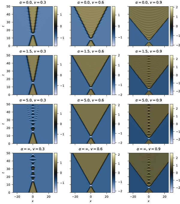
There is also emission of radiation, since the model is not integrable. For small values of , the field behavior around the vacua is well approximated by the Klein-Gordon equation, which is a linear equation. Therefore, the radiation for those cases resemble linear waves. However, as the model becomes more massive, the field around the vacua is better approximated by the signum-Gordon equation, causing the radiation to be more localized. In fact, the radiation spectrum of the signum-Gordon model is known to be dominated by compact oscillons [19].
A more systematic classification of the scattering result as capture or escape can be accomplished without needing to analyze the full simulation results. It is enough to concentrate on the field at the middle point between the kink and the antikink, which is the origin . From the function we can identify the capture cases as the ones in which the field at oscillates indefinitely, while the escape cases correspond to functions that remain close to the vacuum value after a few oscillations. From our simulations we obtained the field at as a function of and for some values of , and present the results in figure 9.
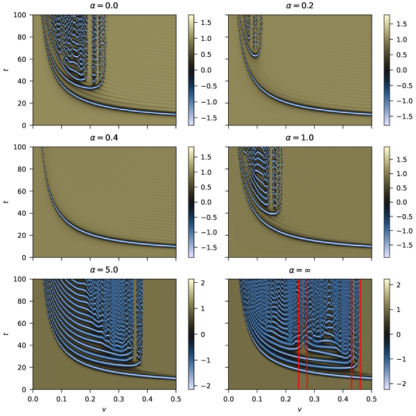
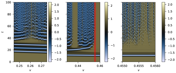
For the case , we reproduce the picture of alternating windows of capture and escape of the model. When we increase the value of to , we see that the range of velocities for which this pattern happens gets narrower. For (), the pattern completely disappears, which means that for all velocities the kink-antikink pair annihilates and reemerges after a single bounce of the field, i.e. there are no capture cases. If we keep increasing the value of , the capture cases reappear. However, as we approach the hyper-massive limit, the pattern of escape windows becomes more straightforward. In the non-analytic case , the capture and escape cases are almost neatly separated, with only two regions (delimited by red lines) with more than one bounce followed by escape, which we highlight in figure 10. However, the transition from the cases of capture to the cases of escape of the kink-antikink pair is not straightforward, and depends on the velocity in a rather subtle way. In the case of compact kinks the transition from capture to escape happens in a fractal manner [20, 14]. In figure 10 we see that this fractal behavior is also present here, suggesting it is a general feature of compact kink-antikink collisions.
At last, we take a more complete picture of the dependency on the potential parameter by looking at the field at the origin on a fixed “final” time, which we set as . When the kink-antikink pair escapes the field will have values close the vacuum value . However, for the capture cases, the field can have values very different due to its oscillatory behavior. Therefore, the color map of as a function of and can indicate the position of capture and escape cases in the parameter space . In figure 11 we present the values of extracted from our simulations.
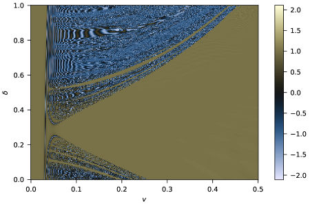
We observe that the capture windows get narrower until completely vanishing for close to . For more massive models, the capture windows reemerge in a pattern which is initially symmetric around the axis . The symmetry stops holding approximately halfway towards the non-analytic case . The range of velocities where the capture cases are contained grows with the mass after its reemergence, and reaches its maximum for the non-analytic case. We also see a band of escape cases (olive color in the plot) emerging between capture windows (blue) and moving to higher velocities as increases. This escape cases are the ones seem in the middle panel of figure 10 for .
The disappearance and reemergence of the capture cases is a rather surprising feature of the transition towards the hyper-massive regime. Since both the and the non-analytic model have similar results for the kink-antikink collisions, one could expect that the transition between them would be more straightforward. The non-monotonic behavior of in relation to changes in indicates that some intricate mechanism happens exclusively for intermediary values of .
V Kink-antikink moduli space
There is a lot of interest in finding effective descriptions of kink-antikink collisions without having to resort to full solutions of the field equations. One approach that has found some success is the construction of kink-antikink moduli space in what is also known as the collective coordinate approximation. Solving the dynamics for the collective coordinates is not necessarily easier than performing the full field simulations. The evaluation of and as well as the time evolution of the equations of motion for are hard computational problems, subject to many nuanced numerical challenges, while the full field theory simulation is a more straightforward problem. However, we still study collective coordinates approximations to the kink-antikink scattering because they allow us to more clearly identify which modes of the field are responsible for the phenomena observed in the full field simulations. On the appendix we discuss more on the steps needed to numerically solve the collective coordinates models discussed below.
We first consider a moduli space where the field is described at all times by a simple superposition of kink and antikink, similar to the initial condition. In this case, we have only one coordinate, the position of the antikink. The configuration is symmetric around , so the field is given by the formula
We call this the non-relativistic case since we do not take the Lorentz contraction into account.
Note that we only have closed form expression for for the cases and . All the other cases have to be treated fully numerically. Since the case is the very widely studied model, we write the metric and potential as functions of for only. For the non-analytic model, we calculate the single metric component to be
while the potential is
These are piecewise functions because they must take into account all the different possibilities for overlapping support of the kink solutions. In figure 12 we present the graph of these functions, together with the numerical results for other values of .
For the non-relativistic model in this section, the position is the only degree of freedom, and therefore it carries all the configuration energy. Since the effective mechanical system has conservation of energy, the motion of is always reflected by the potential , making so that all collisions result in escape of the kink-antikink pair. However, the shape of the potential can still give us insight into the capture cases by imagining that the activation of unaccounted modes or radiation makes lose energy and get trapped at the potential well, oscillating around .
In particular, we can look at the force to understand the higher critical velocity separating the capture from escape case in the non-analytic model in relation to models with smaller masses. Since the force for negative is smaller for higher values of , there is less repulsion between the soliton pair while it bounces. Figure 12 shows that the force grows as goes towards more negative values. However, the slope of is greater for smaller values of . This makes the interaction more repulsive for small when goes to more negative values. Therefore, the soliton pair is more likely to be separated when is small. For the case, the force is constant for , having its maximum value of 8. This is a consequence of the fact that compact kinks do not interact when their support do not overlap. For other , the force keeps growing for more negative because the kinks interact even at large distances. We compare the force for the whole range of at in figure 13. The interaction is indeed more repulsive for small . However, the behavior is monotonically decreasing in , offering no explanation for the absence of capture cases for .
We can improve on the description by adding more kink modes to the field expression. A tentative expression for the field during a kink-antikink collision is a superposition with the first internal mode activated:
The collective coordinates are and , which can be interpreted as the antikink center of momentum and internal mode amplitude, respectively. The function is is any function that behaves as for small , and as for large . A function like this fixes the null-vector problem at while keeping the interpretation of as the amplitude of the internal mode when the solitons are separated [4]. Provided that the above properties are satisfied, the specific choice of does not matter, since cases with different can be mapped through a redefinition of the coordinate . A convenient choice is .
The internal mode can store part of the collision energy, making so that the translational mode gets trapped in the potential well. This translates into the presence of capture cases. Similar to the analysis of the simulation results, we can identify scattering result as capture or escape by looking at the field at the origin . Using the numerical results for and , we calculated for different values of and . In figure 14 we present these results as function of time and scattering velocity for the same selected values of used in figure 9.
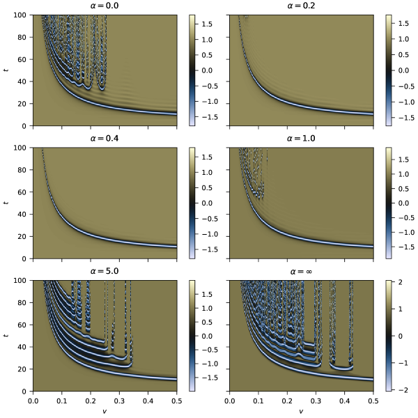
The comparison between the simulation results in figure 9 and the collective coordinates predictions in figure 14 show reasonable agreement. While the collective coordinates model studied here is too simple to be quantitatively predict all features of the field dynamics, it correctly predicted the disappearance and reemergence of capture windows observed in the simulations. Since the only additional coordinate in relation to the previous model is the internal mode amplitude , we can conclude that the first internal mode is the main driver of the dependence of the capture cases on and .
Another important find is that the collective coordinates approach works even though the internal mode makes the field derivative discontinuous at in the non-analytic case. Even though the field equations demands to be continuous, the collective coordinates approach is more flexible because no second order derivative of appears in the metric or the potential. Furthermore, the discontinuity of does not affect the continuity of and due to the integration in the formulas (4) and (5).
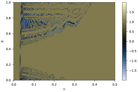
We take a more complete look at the ultimate result of the collision predicted by the collective coordinates approximation in figure 15, where we present the field at and as a function of and . Comparing with the full simulation results in figure 11, we see that the collective coordinates model indeed predicts the lack of capture cases around , although it happens for a wider range of values of . We also see some escape windows happening for regions of the parameter space where the kink-antikink pair should have been captured. This indicates that there are even higher modes, or even radiation, contributing to the presence of annihilation cases. However, the moduli space approach performs reasonably well even though it is a model with only two degrees of freedom.
The collective coordinate models above are non-relativistic in the sense they do not include Lorentz contraction. Introducing a new coordinate to account for the Lorentz contraction, one could propose that the field is once again the superposition
However, this approach generates a null-vector problem because , which makes an entire row and column of the metric null, which in turn makes impossible to solve equation (6).
To sidestep this null-vector problem, it has been proposed that, instead of including the scale factor , one writes and consider the relativistic modes perturbatively [7], using a series expansion like the one in equation (7). However, we replace the coefficients with independent mode amplitudes , so that the field for a single kink is
and kink-antikink configuration can be modeled by the expression
where each is a coordinate, and we once again introduced to avoid a null vector problem.
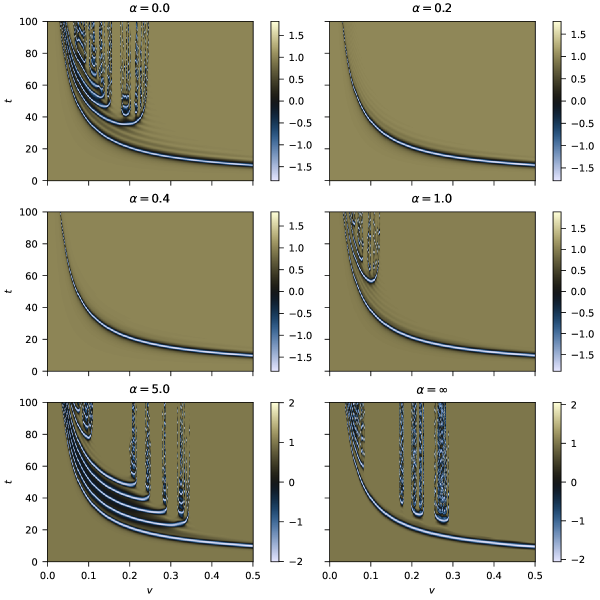
The collective coordinate model with only the first Derrick mode generates similar predictions to the model with the first internal mode, as seen in figure 16. This is expected, because the Derrick mode is very similar to the first internal mode for all , as discussed in section III.
In some scalar field models, the collective coordinates predictions were significantly improved by the addition of higher modes. This means, truncating the sum at some . However, this approach is not possible in the hyper-massive model because is a discontinuous function. Differently to the discontinuity in the first derivative of the internal mode, this discontinuity is in the mode itself, causing a divergence in the metric. Note that, for small
The third derivative of the kink profile is proportional to a Dirac delta in the case . This Dirac delta shows up square in the metric component for , causing a divergence. Therefore, the perturbative approach to relativistic moduli space is limited to the first mode in the hyper-massive regime. Even for finite , as the mass increases, the metric becomes very large and causes numerical difficulties. Therefore, in this work we do not explore coordinates beyond .
VI Conclusions
In this paper we studied how the transition from the traditional model to a model with non-analytic potential influences static and interacting kinks. We did this through a family of potentials parametrized by the mass of small perturbations around the vacua configurations, in a way that allows the non-analytic case to be identified as the infinite mass case. In the non-analytic case, the kink and its internal modes have compact support, i.e. they are non-trivial only inside a compact region of space. We observed that the internal and Derrick modes of the compact kink have identical frequencies to the case of the model. It was also possible to generalize to the whole family of potentials the similarity between the first internal mode and the Derrick mode.
In the case of interaction kinks, we focused on the classification of kink-antikink collision results in escape or capture cases. Our simulations showed that, as the mass increases, the window of velocities containing the capture cases get narrower until eventually disappearing. However, if we continue to grow the mass, the capture cases reappear and their window of velocities grows, reaching its maximum value for the infinite mass case. This rather surprising result suggests that the model and the non-analytic model have more in common with one another than with intermediary models. An explanation for these similarities demands further investigation and is a possible follow up to this work.
To better understand the underlining causes of the capture cases, we analyzed the kink-antikink scattering through a moduli space approach. We found that the inclusion of the first kink internal mode in the description is enough to explain qualitatively the dependence of the capture cases on the collision parameters, including the absence of capture when the potential parameter has values close to 0.3. Similar results hold when replacing the internal mode with the first Derrick mode in a perturbatively relativistic approach. However, we could do not expand the moduli space to include higher Derrick modes due to a discontinuity in such modes in the hyper-massive case. This highlights how, even though the collective coordinate approximation is very useful even in non-analytic models, some techniques developed for more traditional models do not generalize.
Acknowledgements.
We thank R. Thibes for helpful comments and discussions. This study was financed in part by the Coordenação de Aperfeiçoamento de Pessoal de Nível Superior – Brasil (CAPES) – Finance Code 001 and by the Conselho Nacional de Desenvolvimento Científico e Tecnológico – Brasil (CNPq).Appendix A Numerical methods
The numerical work was done using the Julia programming language [21] and the library DifferentialEquations.jl [22].
For the full field equations, we discretize the spatial position with steps and approximate the derivatives using fourth-order finite differences. The resulting coupled second order equation for the variables are evolved in time with a sixth-order Kahan-Li symplectic method [23] with time steps . We used spatial steps ranging from to . Other methods and step sizes were tested and yielded consistent results.
In the collective coordinate approximation, we calculate the integrals for and numerically. Since the calculation of and is computationally expensive, we compute it on a fixed grid for the collective coordinates and obtain the values from a cubic B-spline interpolation. This approach is inspired by the one described in ref. [24]. With the metric and the potential given by such interpolations, we solved the equations of motion for using the velocity Verlet symplectic method [25]. We tuned the numerical algorithms so that increases in the numerical precision (generally trough decreases in step size) did not significantly change the systematic results in figures 14, 15, and 16. Therefore, the overall results represent a physically correct result, even though an independent implementation could find different trajectories for specific cases, leading to differences in the fine details. This is due to the high susceptibility of the collective equations to small changes, since they represent very intricate dynamical systems.
Since the computation of and becomes too expensive for high number of collective coordinates, we limited ourselves to moduli spaces with one or two dimensions by only including the first internal mode. For example, generating figure 15 with a resolution of data points required solving equation (6) a total of 251001 times, as well as finding 501 kink solutions and their internal modes, which lead to 501 different metric and potentials functions, each one calculated from a 176000 point grid. In other works [7, 14] the computation was done at every step of the time evolution, however this approach is also too computationally demanding for our needs, because we need to explore different values of , making the total number of scenarios to be considered way larger than in previous works.
References
- Manton and Sutcliffe [2004] N. Manton and P. Sutcliffe, Topological Solitons, Cambridge Monographs on Mathematical Physics (Cambridge University Press, Cambridge, 2004).
- Kevrekidis and Goodman [2019] P. G. Kevrekidis and R. H. Goodman, Four Decades of Kink Interactions in Nonlinear Klein-Gordon Models: A Crucial Typo, Recent Developments and the Challenges Ahead (2019), arXiv:1909.03128 [nlin] .
- Manton et al. [2021a] N. S. Manton, K. Oleś, T. Romańczukiewicz, and A. Wereszczyński, Collective coordinate model of kink-antikink collisions in theory, Physical Review Letters 127, 071601 (2021a).
- Manton et al. [2021b] N. S. Manton, K. Oleś, T. Romańczukiewicz, and A. Wereszczyński, Kink moduli spaces: Collective coordinates reconsidered, Physical Review D 103, 025024 (2021b).
- Pereira et al. [2021] C. F. S. Pereira, G. Luchini, T. Tassis, and C. P. Constantinidis, Some novel considerations about the collective coordinates approximation for the scattering of kinks, Journal of Physics A: Mathematical and Theoretical 54, 075701 (2021).
- Pereira et al. [2023] C. F. S. Pereira, E. dos Santos Costa Filho, and T. Tassis, Collective coordinates for the hybrid model, International Journal of Modern Physics A 38, 2350006 (2023).
- Adam et al. [2022] C. Adam, N. S. Manton, K. Oles, T. Romanczukiewicz, and A. Wereszczynski, Relativistic moduli space for kink collisions, Physical Review D 105, 065012 (2022).
- Adam et al. [2023a] C. Adam, D. Ciurla, K. Oles, T. Romanczukiewicz, and A. Wereszczynski, Relativistic moduli space and critical velocity in kink collisions, Physical Review E 108, 024221 (2023a).
- Blaschke et al. [2023] F. Blaschke, O. N. Karpíšek, and L. Rafaj, Mechanization of a scalar field theory in 1+1 dimensions: Bogomol’nyi-Prasad-Sommerfeld mechanical kinks and their scattering, Physical Review E 108, 044203 (2023).
- Rosenau and Hyman [1993] P. Rosenau and J. M. Hyman, Compactons: Solitons with finite wavelength, Physical Review Letters 70, 564 (1993).
- Arodź [2002] H. Arodź, Topological compactons, Acta Physica Polonica B 33, 1241 (2002), arXiv:nlin/0201001 .
- Adam et al. [2017] C. Adam, J. Sanchez-Guillen, and A. Wereszczynski, BPS submodels of the Skyrme model, Physics Letters B 769, 362 (2017).
- Klimas et al. [2018] P. Klimas, J. S. Streibel, A. Wereszczynski, and W. J. Zakrzewski, Oscillons in a perturbed signum-Gordon model, Journal of High Energy Physics 2018, 102 (2018).
- Hahne and Klimas [2024] F. M. Hahne and P. Klimas, Scattering of compact kinks, Journal of High Energy Physics 2024, 67 (2024), arXiv:2311.09494 .
- Bazeia et al. [2014] D. Bazeia, L. Losano, M. A. Marques, and R. Menezes, From kinks to compactons, Physics Letters B 736, 515 (2014).
- Arodź et al. [2008] H. Arodź, P. Klimas, and T. Tyranowski, Compact oscillons in the signum-Gordon model, Physical Review D 77, 047701 (2008).
- Hahne and Klimas [2022] F. M. Hahne and P. Klimas, Compact kink and its interaction with compact oscillons, Journal of High Energy Physics 2022, 100 (2022).
- Sugiyama [1979] T. Sugiyama, Kink-antikink collisions in the two-dimensional model, Progress of Theoretical Physics 61, 1550 (1979).
- Hahne et al. [2020] F. M. Hahne, P. Klimas, J. S. Streibel, and W. J. Zakrzewski, Scattering of compact oscillons, Journal of High Energy Physics 2020, 6 (2020).
- Bazeia et al. [2019] D. Bazeia, T. S. Mendonça, R. Menezes, and H. P. de Oliveira, Scattering of compactlike structures, The European Physical Journal C 79, 1000 (2019).
- Bezanson et al. [2017] J. Bezanson, A. Edelman, S. Karpinski, and V. B. Shah, Julia: A Fresh Approach to Numerical Computing, SIAM Review 59, 65 (2017).
- Rackauckas and Nie [2017] C. Rackauckas and Q. Nie, DifferentialEquations.jl – A Performant and Feature-Rich Ecosystem for Solving Differential Equations in Julia, Journal of Open Research Software 5, 15 (2017).
- Kahan and Li [1997] W. Kahan and R.-C. Li, Composition constants for raising the orders of unconventional schemes for ordinary differential equations, Mathematics of computation 66, 1089–1099 (1997).
- Adam et al. [2023b] C. Adam, A. García Martín-Caro, M. Huidobro, K. Oles, T. Romanczukiewicz, and A. Wereszczynski, Constrained instantons and kink-antikink collisions, Phys. Lett. B 838, 137728 (2023b).
- Verlet [1967] L. Verlet, Computer “experiments” on classical fluids. I. Thermodynamical properties of Lennard-Jones molecules, Phys. Rev. 159, 98 (1967).