Uncertainty quantification of optical models in fission fragment de-excitation

Abstract

We take the first step towards incorporating compound nuclear observables at astrophysically-relevant energies into the experimental evidence used to constrain optical models, by propagating the uncertainty in two global optical potentials, one phenomenological and one microscopic, to correlated fission observables using the Monte Carlo Hauser-Feshbach formalism. We compare to historic and recent experimental data, and find that the parametric optical model uncertainty in neutron-fragment correlated observables is significant in observables involving neutron energies and multiplicities. Different phenomenological and microscopic potentials disagree, both with experiment and with each other, which we attribute to the extrapolation of the phenomenological models away from stability, and to the limitations of the nuclear matter folding approach for the microscopic model. We comment on the role of the optical model in future efforts to globally optimize fission models.

I Introduction

How nucleons organize themselves across the nuclear chart, including the origin of heavy isotopes in the astrophysical r-process, requires understanding of nuclear reaction phenomenology away from stability Hebborn et al. (2022a); for the Horizon: The 2015 Long Range Plan for Nuclear Science (2015). The extrapolation of reaction models into the region of fission fragments is specifically necessary for predictive cross sections required for r-process simulations, nuclear non-proliferation and forensics applications and for modeling the fission process itself. In particular, accurate fission event generators are important to nuclear science and technology, for the interpretation of experimental fission observables, and for evaluation of prompt fission neutron spectrum (PFNS) for actinides Trkov et al. (2015); Capote et al. (2016). Monte Carlo Hauser-Feshbach (MCHF) codes are commonly employed in these efforts, as fission produces multiple correlated signatures Lovell and Neudecker (2021, 2022); Talou et al. (2021).

The typical workflow for nuclear reaction phenomenology often involves constraining a global nucleon-nucleus optical model potential (OMP) to elastic scattering experiments on $\beta$-stable targets, and then extrapolating away from stability to the neutron-rich region, for which experimental data are unreliable or non-existant. Global phenomenological OMPs provide workhorse models for the nucleon-nucleus interactions that are key ingredients in the formalism for direct and compound reactions. However, extrapolating away from the isotopic and energy regions for which they are fit introduces un-quantified uncertainty. This need for extrapolation is exemplified in Fig. 1, in which the isotopes used to constrain a workhorse global phenomenological optical potential Koning and Delaroche (2003) are compared to fission fragment yields.

In particular, the imaginary surface component of the optical potential is peaked at low energies, reflecting that low-energy neutrons are preferentially absorbed, and emitted, from the fringe regions of the nucleus, where nucleon density, and, therefore, Pauli blocking effects, are diminished relative to the interior Moldauer (1962). Understanding the isovector ($\alpha=\pm\frac{N-Z}{N+Z}$) dependence of this low-energy imaginary surface strength, where the plus (minus) sign is for incident protons (neutrons), is essential for astrophysical applications, with simulations predicting a strong sensitivity of r-process reaction rates to the isovector dependence, especially for drip-line nuclei Goriely and Delaroche (2007). Moreover, the symmetry energy of nuclear matter, as well as its first order density dependence about saturation density,is contained in the nucleon optical potential; in particular the energy dependence and isovector component Xu et al. (2010).

A key ingredient in nuclear reaction modeling away from stability are global OMPs, the Hauser-Feshbach formalism for decay chains of compound nuclei being no exception. This motivates the quest for predictive phenomenology away from the line of stability. The advent of the rare isotope beam era has begun to widen the experimentally accessible region of the isotopic chart, with significant increases still to come Bollen (2010). The development of uncertainty-quantified OMPs that are predictive for these rare isotopes has been the subject of a recent corresponding theoretical effort Hebborn et al. (2022a). Simultaneously, there has been a focus on applying rigorous uncertainty quantification using Bayesian statistics to the calibration of phenomenological optical potentials Lovell and Nunes (2018); King et al. (2019); Catacora-Rios et al. (2019); Lovell et al. (2020); Catacora-Rios et al. (2021); Pruitt et al. (2023).

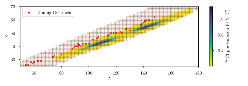
Figure 1: Chart of isotopes in the fission fragment region, where the isotopes used to constrain the commonly used Koning-Delaroche phenomenological neutron-nucleus global optical potential Koning and Delaroche (2003) (red squares) are compared to ²⁵²Cf$(sf)$ pre-emission fragment yield distributions, as generated by CGMF Talou et al. (2021).

Most of these efforts calibrate the optical potential parameters to elastic scattering experiments. The corpora of experimental data typically include include neutron and proton differential elastic scattering cross sections, $d\sigma/d\Omega$, and total and reaction cross sections, $\sigma_{t}$ and $\sigma_{r}$, respectively, as well as analyzing powers. Current work has focused on propagating OMP uncertainties into specific non-elastic reaction channels, such as charge-exchange and knockout reactions, with the goal of eventually including non-elastic measurements as OMP constraints in the form of Bayesian posteriors for model calibration Whitehead et al. (2022); Hebborn et al. (2022b); Smith et al. (2024).

In this work, we propose the expansion of this corpus to include compound nucleus (CN) observables in which unstable nuclei are produced, directly into the calibration likelihood for OMPs. Specifically, we focus on observables from fission. This has several potential advantages:

1. measurements of fission fragments and their prompt emissions provide experimental access to unstable nuclei, thereby directly testing the extrapolations of global OMPs from stability,

2. the energy scale of prompt neutron emissions is typically closer to astrophysically relevant energies than direct reactions in beam-line experiments,

3. and there already exists a large library of historical experimental data for fission-fragment decay spectroscopy, including correlations

It is also worth noting that CN processes already contaminate elastic scattering measurements at low incident nucleon energy, where compound-elastic processes dominate the cross sections. In one way or another, all phenomenological OMPs that extend to low energies must address this in the calibration. Due to computational limitations, the approximation may be adopted to pre-calculate the CN-elastic cross section with a Hauser-Feshbach (HF) treatment, using a single set of OMP parameters from the prior; that is, the CN-elastic component is typically not adjusted with the calibration Pruitt et al. (2023).

Directly incorporating CN observables, including fission, potentially provides new constraints for phenomenological OMPs at low-energy, that may be underconstrained currently. The sensitivity of CN reaction formalisms to model inputs has been tested in the past; e.g. for non-statistical properties Kawano et al. (2021) in fission, and for level densities in fusion Voinov et al. (2007).

It is a computationally demanding task to simultaneously quantify uncertainty and correlations between all model inputs for every CN observable of interest, but the piecemeal efforts so far have indicated strong sensitivity to level densities and cases where results disagree significantly with experiment Voinov et al. (2007). This indicates the potential efficacy of optimizing model inputs — level densities, OMPs, strength functions, etc. — to CN observables; and, indeed, level densities have previously been extracted from neutron evaporation spectra, Wallner et al. (1995); Ramirez et al. (2013) to name a few. It has been suggested that uncertainties in CN observables due to the OMP may be larger than for level densities in some cases; particularly at low energy Pruitt et al. (2023). Therefore, we take the first steps here to quantify this uncertainty in fission.

Nuclear fission has been a subject of study since its discovery by Lise Meitner and Otto Frisch in the experimental results of Otto Hahn in 1938. The phenomenon, in which a fissile nuclide - typically an actinide - deforms into an unstable configuration which splits into (typically) two fragments, produces a variety of correlated observables, and spans many orders of magnitude in time.

Due to the interesting, still not fully understood, physical phenomena associated with fission, and the importance of the reaction to society, it has been subject to extensive measurement and modeling (For an exhaustive review see Talou and Vogt (2023); Schunck and Regnier (2022) and references therein). The observables we consider in particular are the prompt neutrons emitted from the fragments as the de-excite, which are strongly correlated with the excitation energy and angular momentum of the fragments following scission, as well as the branching ratios for de-excitation.

There is a rich history of experiments investigating the properties and correlations between the prompt emissions in fission going back at least six decades Schmitt et al. (1965); Marin et al. (2020); Oberstedt et al. (2013); Wilson et al. (2021); Hoffman (1964); Franklyn et al. (1978); Budtz-Jørgensen and Knitter (1988). Measured observables include the energy and multiplicity of neutrons and photons, and the correlations between them and the fragments themselves. Fission experiments present a breadth of data which can potentially constrain OMPs.

Simultaneously, it is desirable to understand the model dependence of predictions of fission codes. The pre-emission fragment states cannot be directly measured, and the effect of the dependence on the de-excitation model of reconstructions of the pre-fragment state must be well understood to use experiments to probe open questions about excitation energy and angular momentum sharing in fission Wilson et al. (2021). Specifically, it has been observed that OMP predictions of the removed angular momenta of emitted neutrons is larger than expected Stetcu et al. (2021).

The post-scission fragment is born into a state dependent on the conserved quantities (mass, charge, angular momentum, excitation energy, etc.) of the pre-scission compound nucleus, its deformation at the saddle point, and the dynamics of scission. It then equilibrates its excess deformation energy into excitation energy and, typically, promptly emits a neutron or two. Once its residual excitation energy approaches the neutron separation energy, photon emission will strongly compete with neutrons, as the fragment continues to de-excite through statistically distributed levels. Once the excitation energy and parity of the fragment reaches the Yrast line, discrete photons are emitted, carrying away the majority of the fragments excess angular momentum. Following this prompt de-excitation, the residual fragment will often remain $\beta$ un-stable, leading to further delayed emissions and long-lived products.

It is the goal of this work to determine, to what degree, that measurements of the prompt emissions provide constraints on the nucleon-nucleus interaction between the residual fragments and their neutron progeny. We investigate this dependence for the first time by propagating two uncertainty-quantified OMPs through MCHF fission fragment de-excitation with the CGMF code, and constructing credible distributions for a variety of fission observables. These distributions represent the uncertainty of a given fission observable, due to the parametric uncertainty in an OMP.

The paper is organized as follows: in section  II, we briefly review the theory of nucleon evaporation from an excited nucleus. In section  III, we discuss the implementation of this theory in CGMF and the observables considered, and in  IV, we report and discuss results, discussing in detail the disagreements between the different OMPs and theory. Finally, in section  V, we comment on the sensitivity of fission observables to OMPs, as well as discuss future work directly incorporating these observables as constraints, and in the global optimization of model inputs into CGMF, enumerating the assumptions required to do so.

II Theory of nucleon emission from an excited nucleus

Calibrating an optical potential to CN observables of a given reaction is reasonable to propose if (1) the HF formalism (or an extension of it) sufficiently describes the reaction and (2) the reaction explores a phase space (e.g. in mass, charge and energy) not available in typical elastic scattering experiments. As discussed, the latter is clearly true for fission. In this section we discuss the former; briefly reviewing the HF theory of the CN to clarify the connection between the OMP and the decay of the CN, and clearly enumerate the assumptions that are made so that this connection may be utilized only when applicable. The bulk of the formalism developed in this section is included in standard textbooks on reaction theory, e.g. Thompson and Nunes (2009), but we specialize the discussion to its application to fission fragments.

Prompt neutron emission is governed by the initial state of the fragment after scission, as well as the level density of the residual core, and the matrix element for the emission. In particular, consider the state of the emitted nucleon, with asymptotic kinetic energy $E=\hbar^{2}k^{2}/2\mu$:

$$\begin{split}\ket{kjl}&\equiv\ket{k}\sum_{m}\mathcal{Y}^{m}_{jl}\\ &=\ket{k}\sum_{m_{s}m_{l}}i^{l}\braket{lsm_{l}m_{s}}{jm}Y_{l}^{m_{l}}\chi_{s}^{m_{s}}\end{split}$$ (1)

with $\mu$ being the reduced mass of the system. Here, $l$, $s=1/2$ and $j$ respectively label the orbital, spin and total angular momentum quantum numbers, with $m_{l}$, $m_{s}$ and $m$ their respective projections. $\chi_{s}^{m_{s}}$ is the spin wavefunction, $Y_{l}^{m}$ are the orbital wavefunctions, e.g., the spherical harmonics, and $\mathcal{Y}_{l}^{m_{l}}$ are the corresponding spin-orbital angular wavefunctions.

The probability of emitting a neutron described by this state from a CN system with total spin $I$ and parity $\pi$ is given by the transmission coefficient, $\mathcal{T}_{jl}^{I\pi}$, which is defined as

$$T_{jl}^{I\pi}(E)=1-|\mathcal{S}_{jl}^{I\pi}(E)|^{2},$$ (2)

where the partial wave $\mathcal{S}$-matrix is due to the effective interaction between the neutron and the residual core, the OMP.

Our scenario of interest is an initial $A+1$ nucleus in some eigenstate $m$ with energy $E_{m}^{A+1}$ and total angular momentum $I_{m}$ emitting a nucleon to leave the residual $A$-body core in a state $n$ with energy $E_{n}^{A}$ and total angular momentum $I_{n}$. The neutron-removal threshold is $S^{A+1}_{N}=E_{0}^{A+1}-E_{0}^{A}$, where $n=0$ refers to the ground state of the respective system. Of course, energy, parity and total angular momentum are symmetries of the center-of-mass (COM)-frame Hamiltonian, so we have a triangular sum rule for total angular momenta:

$$|I_{n}-j|<I_{m}<I_{n}+j,$$ (3)

as well as conservation of energy: neutron emission with energy $E$ in COM-frame, leaves the excited residual core with energy $E_{n}^{A}$, such that

$$\begin{split}E_{m}^{A+1}&=E_{n}^{A}+E\\ E_{x}^{A+1}-E_{x^{\prime}}^{A}+S_{N}^{A+1}&=E,\end{split}$$ (4)

where $E_{x}$ refers to excitation energy above the corresponding ground state.

The formula for the probability (or fractional width) for the compound nucleus to de-excite through this channel is the ratio of the corresponding transmission coefficient to the sum of those to all open channels:

$$\begin{split}p(\alpha)&=\frac{\Gamma_{\alpha}}{\sum_{\beta}\Gamma_{\beta}}\equiv\frac{\Gamma_{\alpha}}{\Gamma}\\ &=\frac{\mathcal{T}_{\alpha}}{\sum_{\beta}\mathcal{T}_{\beta}},\end{split}$$ (5)

this is the Hauser-Feshbach theory Hauser and Feshbach (1952). Here $\Gamma_{\alpha}$ refers to the $\alpha$ channel decay width, which is proportional to the corresponding transmission coefficient (up to normalization), neglecting width fluctuation correction factors (e.g. assuming no correlation between the entrance and exit channel) Satchler (1963).

Where we do not have information on individual discrete levels, we turn the sum in Eq. (5), which is over channels $n$ with definite COM-frame energy $E_{n}$, into an integral

$$\begin{split}\sum_{n}\mathcal{T}(E=E_{m}^{A+1}-E_{n}^{A})&\rightarrow\int dE_{n}^{A}\left(\frac{dn}{dE_{n}^{A}}\right)\mathcal{T}(E_{m}^{A+1}-E_{n}^{A})\\ &=\int dE_{x}^{A}\underbrace{\left(\frac{dn}{dE_{x}^{A}}\right)}_{\rho(E_{x}^{A})}\mathcal{T}(E),\end{split}$$ (6)

which defines the level density $\rho(E_{x}^{A})dE_{x}^{A}$ of the residual core as a function of excitation energy above the core ground state. We have, by conservation of energy, the residual excitation energy of the core $E_{x}^{A}=E_{x}^{A+1}+S_{N}^{A+1}-E$. This allows us to re-write Eq. (5), expressing the fractional width for neutron evaporation as

$$p(E,j,I_{n},\pi_{n})=\frac{\mathcal{T}_{jl}^{I_{n}\pi_{n}}(E)\;\rho_{jl}^{I_{n}\pi_{n}}(E_{x}^{A+1}+S_{N}^{A+1}-E)}{\sum_{j^{\prime}I^{\prime}\pi^{\prime}}\int dE^{\prime}\;\mathcal{T}_{j^{\prime}l^{\prime}}^{I^{\prime}\pi^{\prime}}(E^{\prime})\;\rho_{j^{\prime}l^{\prime}}^{I^{\prime}\pi^{\prime}}(E_{x}^{A+1}+S_{N}^{A+1}-E^{\prime})}.$$ (7)

This is the central result of the Hauser-Feshbach theory, and is used to model the emission of neutrons from an excited CN. Here, the superscript $I\pi$ implies the limitation to states $jl$ in the subscript that satisfy the triangle relation Eq. (3), and conserve parity. Resolved discrete excited states of the residual core may be included by keeping them in a discrete sum. In practice, the continuum is discretized into uncoupled bins. The sum in the denominator runs over all open channels that respect the symmetries of the system. Equation  (7) can also include photon emission in full competition with neutrons, with $\mathcal{T}_{jl}^{I\pi}$ also representing the photon transmission coefficient, e.g. as calculated according to giant resonance parameters (see Talou et al. (2021)).

One can use Eq. (7) to model the decay chain of compound nuclei. Decay by nucleon emission requires as ingredients only the level density of the residual core, and the OMP that describes the effective interaction between the residual core and the emitted nucleon.

In this way, given an initial nucleus with well-determined excitation energy, spin and parity, one can compute the probability to decay via a specific mode to a residual nucleus with another excitation energy, spin and parity, and an emitted species of radiation. In fact, the probability in Eq. (7) defines a Markov process, in which the current state of the system (e.g. $A,Z,E,J,\pi$) solely determines its probability of evolving to the next state. By sampling from this probability, one can generate an ensemble of histories, each specifying a trajectory of de-excitation, beginning with an initial excited nucleus, and ending in a stable (or long-lived) state. From many such histories, one can reconstruct experimental observables relating to the emitted radiation, including full correlations between energy, angle, multiplicity and species, as well as with the remaining stable or long-lived nuclei that are produced. This is called the Monte Carlo Hauser-Feshbach (MCHF) formalism, and we discuss it more detail in the next section.

III Uncertainty propagation in Monte Carlo Hauser Feshbach

In this section we discuss the methodology for generating posterior predictive distributions of fission observables due to two different optical potentials using the MCHF method as implemented in the code CGMF. The potentials considered in tihs work are the phenomenological Koning-Delaroche uncertainty quantified (KDUQ) Pruitt et al. (2023); Koning and Delaroche (2003) and the microscopic Whitehead-Lim-Holt (WLH) Whitehead et al. (2021). The fission reactions under consideration were ²⁵²Cf$(sf)$ and ²³⁵U$(n_{\rm{th}},f)$.

III.1 Optical potentials

The KDUQ phenomenological global potential Pruitt et al. (2023) was fit to differential elastic scattering cross sections and analyzing powers, proton reaction cross sections, and neutron total cross sections. It is an uncertainty-quantified version of the workhorse phenomenological OMP Koning-Delaroche Koning and Delaroche (2003), and updates the original potential using a full Bayesian calibration and outlier rejection. The original potential is valid for 1 keV up to 200 MeV, for (near-) spherical nuclides in the mass range $24\leq A\leq 209$. The default parameterization of Koning-Delaroche, as provided in Koning and Delaroche (2003), is the default OMP in CGMF.

In Pruitt et al. (2023), two different likelihood models are used, the “democratic" and the “federal". In the democratic ansatz, the data covariance in the likelihood function is assumed to be diagonal, the experimentally reported uncertainties for each data point are augmented with an unreported uncertainty (estimated in an observable-by-observable basis) and the covariance is scaled by $k/N$, $k$ being the number of model parameters (46), and $N$ being the total number of data points. In the federal ansatz, the data covariance is modified so that data points of observable $i$ are scaled separately by the number of data points belonging to that observable, e.g., by $k/N_{i}$. Thus, each observable has equal influence in the likelihood, and each data point has equal influence within its observable. In Pruitt et al. (2023), the two ansatze produced similar calibrated models, and the federal ansatz is used in this work.

The WLH microscopic global potential was developed in a nuclear matter folding approach Whitehead et al. (2021). First, in asymmetric nuclear matter, at a variety of densities and asymmetry parameters $\alpha$, the single-nucleon self-energy was calculated self-consistently to 2${}^{\text{nd}}$ order in many-body perturbation theory (MBPT), using nucleon-nucleon forces from Chiral effective field theory ($\chi$EFT). These density-dependent self-energies are calculated for a much wider range of asymmetries than is possible in phenomenological models like KDUQ.

The nuclear matter self-energies are then folded to nuclear density distributions using the improved local density approximation (I-LDA) to produce optical potentials. The nucleon densities are calculated in mean-field theory with Skyrme effective interactions Lim and Holt (2017). The underlying theoretical uncertainty was approximated by the spread in resulting parameters from five different choices of chiral interaction. The WLH spin-orbit term was developed using a density-matrix expansion at the Hartree-Fock level Holt et al. (2011).

The targets considered spanned 1800 nuclei, ranging in mass from $12<A<242$, inclusive of light and medium-mass bound isotopes out to the neutron drip line. The energy considered was $E\in[0,200]$ MeV.

For target nuclei with small proton-neutron asymmetry, the WLH isospin-dependence follows the Lane form with first-order $\alpha$ dependence, however, for nuclei with larger isospin asymmetries, the WLH potential contains terms with no parallel in KDUQ, which are proportional to the square of the isospin asymmetry, and strongest at low energy. Understanding the phenomenological implications of these higher order terms is especially interesting for neutron-rich nuclei.

III.2 Monte Carlo Hauser-Feshbach (MCHF)

CGMF Talou et al. (2021) is a MCHF code which generates initial configurations for the fission fragments in mass, charge, kinetic energy, excitation energy, spin, and parity, and then samples their de-excitation trajectories by emission of neutrons and $\gamma$ rays according to Eq. (7). It is capable of neutron induced fission on various actinides over incident energies ranging from thermal to 20 MeV, as well as spontaneous fission of selected isotopes.

CGMF samples the initial post-scission fragment masses using a three-Gaussian model for the distribution in mass number, with energy-dependent centers and standard deviations. The energy dependence is tuned to experimental data. The fragment charges are then sampled conditional on the masses using the Wahl systematics Wahl (1980), and the total kinetic energy (TKE) of the fragments are sampled from a Gaussian using a mass-dependent mean and standard deviation tuned to available data otherwise. The total excitation energy (TXE) is then available by energy balance: $\rm{TXE}=Q_{f}-\rm{TKE}$, where $Q_{f}$ is the energy liberated in the fission, depending on the binding energies of the pair of fission fragments created. The partitioning of the excitation energy is done in the Fermi-gas model, in which the temperature ratio of the light to heavy fragment is allowed to be mass dependent and tuned to prompt neutron properties. The fragment spins are uncorrelated and chosen from Gaussians centered on the number of geometric levels $J(J+1)$, with width tuned to prompt photon properties. Parity states are assumed to be equiprobable.

Once the post-scission states of the two fission fragments for a history have been sampled, they are then de-excited in the MCHF formalism, where the decay of the CN is treated as a Markov process, governed by Eq. (7), with neutron and photon emission in full competition. The MCHF algorithm, given the conserved quantum numbers of the fully-accelerated post-scission fragment, samples from Eq. (7), emitting neutrons and photons until a state is reached that is stable against prompt emissions. The observables are then re-constructed using the event by event information.

The nuclear level density appearing in Eq. (7) is modeled using the Kawano-Chiba-Koura (KCK) systematics, which extends the Gilbert-Cameron model to include an energy dependent level density parameter and defines the procedure for assigning spin and parity to discrete levels for which it is unknown Kawano et al. (2006). Level density models represent another potentially large contributor of uncertainty, as they are plagued by the same issue as OMPs of extrapolating away from stability where data is available.

It is important to note that certain model inputs (e.g. nuclear temperatures used for excitation energy sharing) in CGMF have been tuned to experimental observables, especially mean neutron multiplicities. This tuning was performed using the default Koning-Delaroche (KD) OMP parameterization, so correlations between these parameters and OMP parameters may be responsible for canceling errors in both. This point will be emphasized in the interpretation of the results.

III.3 Posterior predictive distributions of fission observables

For each of the fissioning isotopes considered, the uncertainty propagation was done by brute force, with 300 samples from the posterior distributions of each OMP. In this case of WLH, these samples were generated by assuming a multi-variate normal distribution and sampling from the covariance provided in Whitehead et al. (2021). It should be noted that, although the posterior distributions for WLH are expected to be well approximated by a multi-variate normal, this approximation may lead to a slightly higher proportion of samples drawn from the tails of the distribution. For the case of KDUQ, these samples were taken from the supplemental material of Pruitt et al. (2023), using the federal posterior formulation. For each OMP sample, an ensemble of one million Monte Carlo histories were generated, from which first and second moments of aggregate observables were re-constructed to compare to experiment.

The distribution of values for a given fission observable across histories with a single OMP sample resulted from the inherent Monte Carlo uncertainty, $\sigma_{mc}$. The distribution of mean values across samples represented an estimate of uncertainty due to the OMP, with noise due $\sigma_{mc}$. The uncertainties reported as bands in the results result from the quadrature subtraction of the former from the latter, to estimate the uncertainty due only to the varying OMP parameters. For more details, see App. A.

Within a given ensemble, histories were run in parallel using the MPI implementation in the python module mpi4py Forum (1994); Dalcín et al. (2005). A modified version of CGMF was used with Python bindings, and all software used to run CGMF and analyze results is open-source and available online under the name ompuq . An open-source code for uncertainty-quantification in few-body reaction calculations by the authors called OSIRIS Beyer was used as a dependency within CGMF. OSIRIS accepts as input a set of global optical potential parameters, including for KDUQ and WLH (e.g. in a json file according to the format used by the TOMFOOL code Pruitt et al. (2023) which was used to calculate KDUQ). Insofar as was possible, all components in the software stack created by the authors employ unit and regression testing using pytest Krekel et al. (2004) and Catch2 Hořeňovský (2024).

The propagation of uncertainties through CGMF was a significant computational task. Calculating fission observables for a single parameter sample (consisting of one million CGMF histories) required roughly 30 cpu-hours on the Great Lakes cluster at the University of Michigan, using Intel(R) Xeon(R) Gold 6140 CPUs. The 300 samples required to generate a posterior predictive distribution of observables corresponding to a single potential and fissioning system therefore each required roughly 9300 cpu-hours.

IV Results

IV.1 Prompt neutron observables

The prompt neutron observables refer to those in which only the neutrons need be measured, not the fragments as well. These include neutron multiplicity and energy distributions.

Figure 2 displays $\bar{\nu}$, the mean prompt neutron multiplicities per fission event (inclusive of both fragments) for both OMPs as compared to a variety of experiments and evaluations. In each of these cases, the $\sigma_{mc}$ in each ensemble was negligible compared to the parametric uncertainty of each OMP, and are therefore not shown. For comparison are a variety of experimental results and evaluations of $\bar{\nu}$. Interestingly, each OMP disagreed with each other to statistical significance, with KDUQ generally being the closest to experiment. WLH universally predicted too large of multiplicities.

This can be interpreted from an energy budget perspective, as shown below (see Fig. 3 for example), the WLH optical potential produces softer spectra. For a given initial excitation energy, less energy removed per neutron implies a larger $\bar{\nu}$. Of course, as mentioned, parameters in CGMF relating to the fragment initial conditions are tuned to experiment assuming the default Koning-Delaroche OMP. That is to say, we can only say that the two OMPs are different to statistical significance, not that one is more accurate than the other.

In figures other than Fig. 2, the light and dark shaded regions respectively represent a credible interval of one and two standard deviations for each OMP ($\sigma_{omp}$), the total shaded regions in the figures represent the total uncertainty $\sigma_{t}$, and the grey portions $\sigma_{mc}$ (see App. A). For most observables, the grey bands are negligible, indicating reasonable estimation of the actual OMP parameter uncertainty.

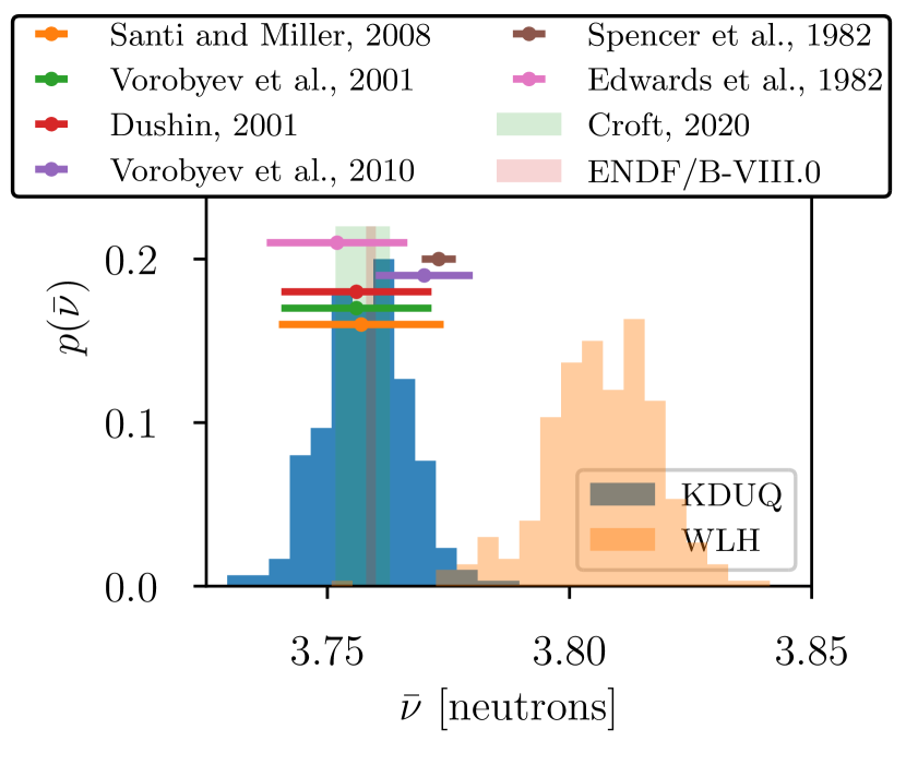
(a) ²⁵²Cf$(sf)$

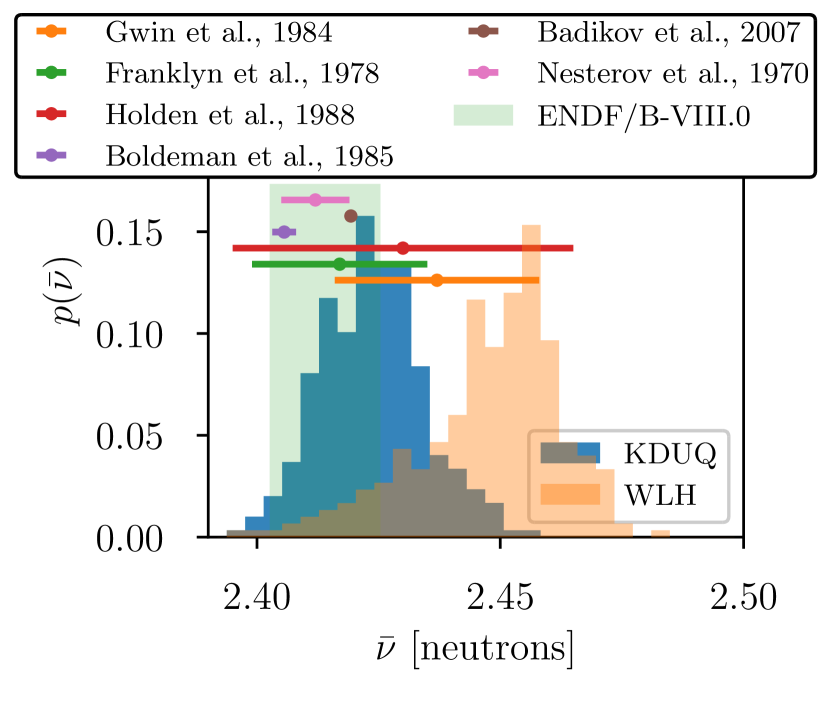
(b) ²³⁵U$(n_{\rm{th}},f)$

Figure 2: Distribution of average prompt neutron multiplicities, $\bar{\nu}$, produced by the uncertainty-quantified OMPs. (a) $\bar{\nu}$ in ²⁵²Cf$(sf)$, compared to evaluations from Croft et al., Croft et al. (2020), and ENDF/B-VIII.0 Brown et al. (2018), as well as experimental results from Santi and Miller (2008); Vorobyev et al. (2010); Dushin et al. (2004); Vorobyev (2001); Spencer et al. (1982); Edwards et al. (1982). (b) $\bar{\nu}$ in ²³⁵U$(n_{\rm{th}},f)$, compared to the ENDF/B-VIII.0 evaluation Brown et al. (2018), as well as experimental results and other evaluations Gwin et al. (1984); Franklyn et al. (1978); Holden and Zucker (1988); Boldeman and Hines (1985); Carlson et al. (2009); Kikuchi et al. (1977).

Figures 3 and 4 display the lab-frame PFNS for ²⁵²Cf$(sf)$ and ²³⁵U$(n_{\rm{th}},f)$ compared to a variety of measurements, all as ratios to a Maxwellian. Clearly, both models predict spectra that are too soft as compared to measurements, WLH especially so. In the 1-10 MeV region, the bands for the two OMP uncertainties are well separated, especially for ²³⁵U$(n_{\rm{th}},f)$.

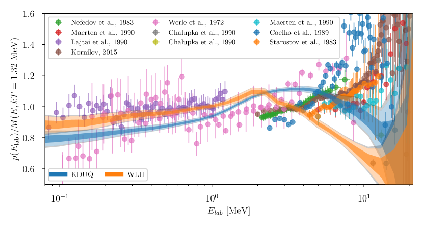
Figure 3: PFNS in the lab frame for ²⁵²Cf$(sf)$ as a ratio to a Maxwellian at $kT=1.32$ MeV, compared to experimental results from Märten et al. (1990); Nefedov (1983); Lajtai et al. (1990); Kornilov (2015); Werle and Bluhm (1972); Chalupka et al. (1990); Coelho et al. (1989); Starostov et al. (1983).

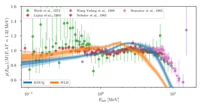
Figure 4: PFNS in the lab frame for ²³⁵U$(n_{\rm{th}},f)$, as a ratio to a Maxwellian at $kT=1.32$ MeV, compared to experimental results from Werle and Bluhm (1972); Lajtai et al. (1986); Yufeng et al. (1992); Nefedov (1983); Starostov et al. (1983).

IV.2 Prompt neutron-fragment correlations

We turn our attention now to experiments in which neutrons and fragments were measured simultaneously. These represent a much smaller, yet highly informative, set of experiments. Neutron-fragment correlations provide detailed information about the fragments immediately after scission, i.e. the neutron multiplicity sawtooth observed by a variety of experimental groups and displayed in Fig. 5. The behavior of $\bar{\nu}(A)$ indicates roughly the allocation of excitation energy ($\bar{\nu}$ being an approximate surrogate) between fragments. Both OMPs reproduce well the expected sawtooth behavior. For most mass numbers, this observable is not strongly correlated to the OMP parameters, with the exceptions of the highly asymmetric region for both fissioning isotopes, and the highly symmetric region for ²³⁵U.

Figure 6 displays the mean single-fragment $\bar{\nu}$ as a function of the TKE of both fragments, compared to a variety of measurements. For both fissioning isotopes, this observables is uncorrelated to the parameters in either model, except for in the low TKE highly symmetric fission region. This region corresponds to highly deformed fragments post-scission, and, therefore, excitation energy dominated systems during de-excitation. Both models reproduce experiment well, especially the most recent measurement by Göök Göök et al. (2014). The lack of correlation to the OMP of $\bar{\nu}$ conditional on fragment mass and TKE indicates the utility of these observables for inclusion as constraints of the global optimization of model inputs unrelated to the OMP, especially those related to scission, e.g. the excitation energy partitioning. In general, the observables relating to the correlations between fragment mass/TKE and neutron multiplicity do not show strong sensitivity to the OMP parameters, and both models agree, with much smaller differences between the two models than between experiments.

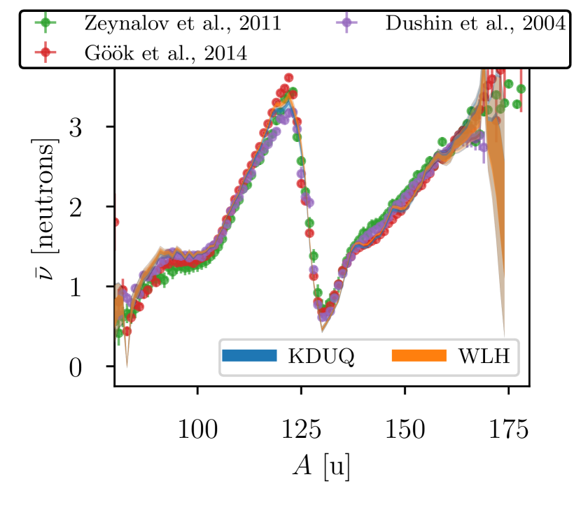
(a) ²⁵²Cf$(sf)$

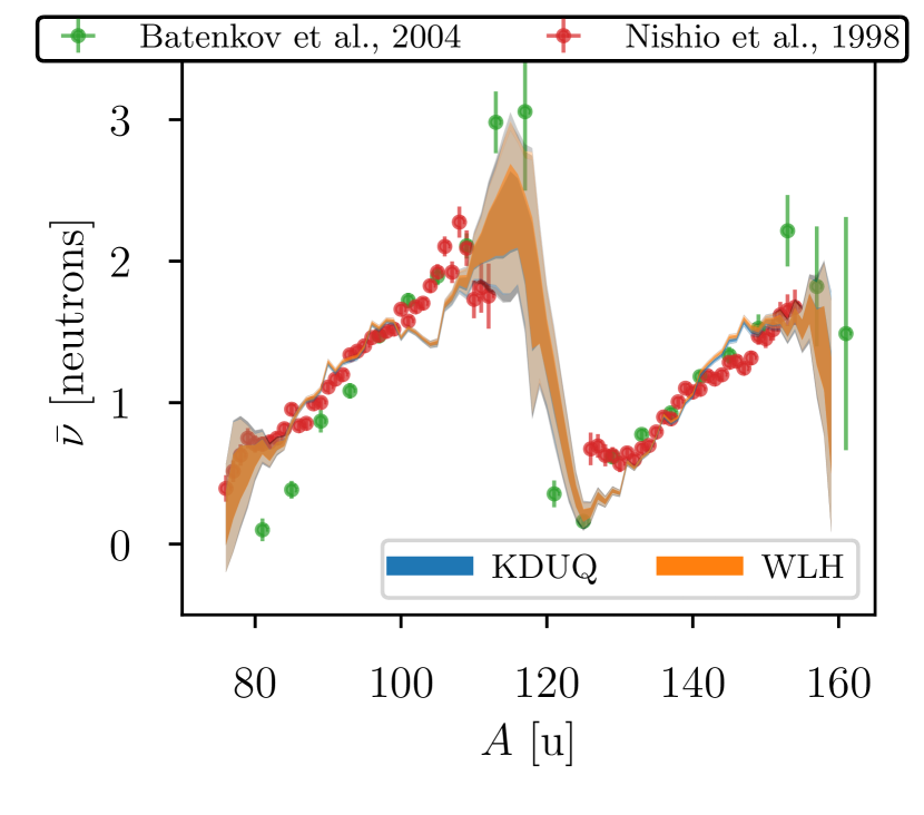
(b) ²³⁵U$(n_{\rm{th}},f)$

Figure 5: Average neutron multiplicity from fragments of a given mass number for (a) ²⁵²Cf$(sf)$ compared to experimental results from Zeynalov et al. (2009); Budtz-Jørgensen and Knitter (1988); Bowman et al. (1963); Ding et al. (1984); Göök et al. (2014); Dushin et al. (2004), and (b) ²³⁵U$(n_{\rm{th}},f)$ compared to experimental results from Batenkov et al. (2005); Nishio et al. (1998)

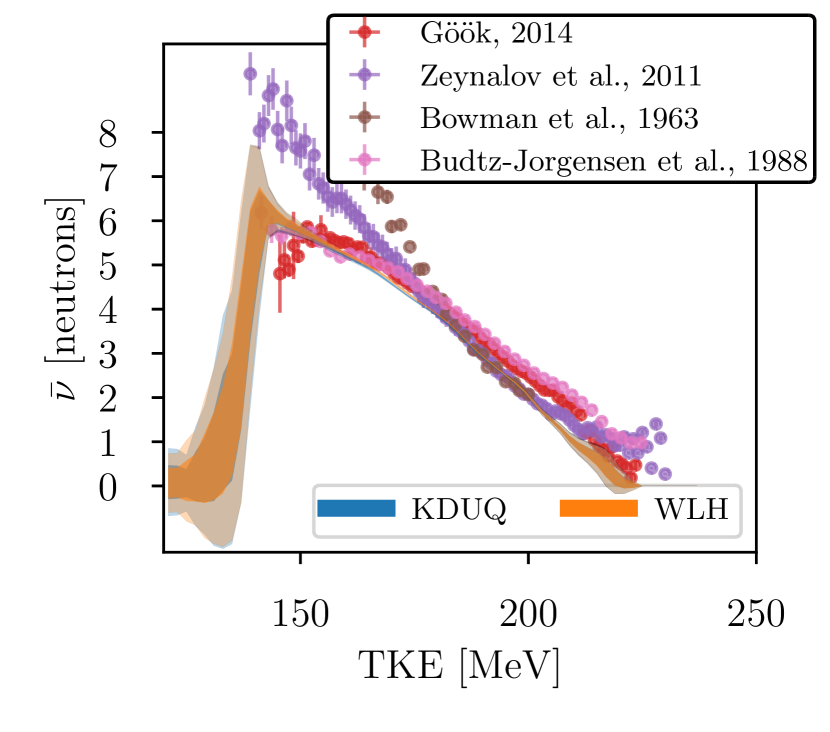
(a) ²⁵²Cf$(sf)$

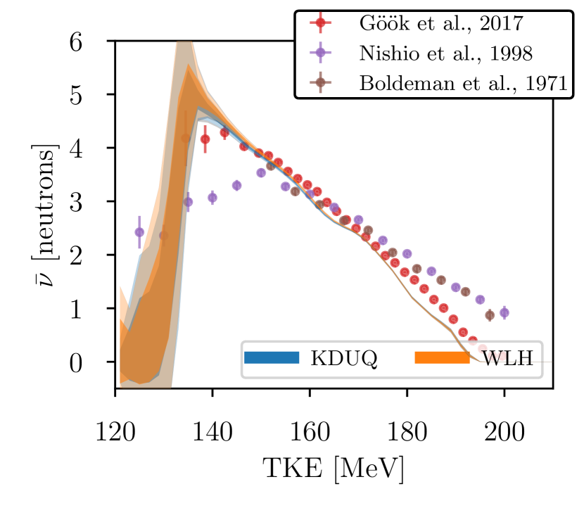
(b) ²³⁵U$(n_{\rm{th}},f)$

Figure 6: Average neutron multiplicity as a function of TKE of the fragments for (a) ²⁵²Cf$(sf)$ compared to experimental results from Göök et al. (2014); Zeynalov et al. (2009); Bowman et al. (1963); Budtz-Jørgensen and Knitter (1988), and (b) ²³⁵U$(n_{\rm{th}},f)$ compared to experimental results from Göök et al. (2018); Nishio et al. (1998); Boldeman et al. (1971)

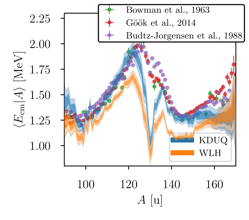
(a) ²⁵²Cf$(sf)$

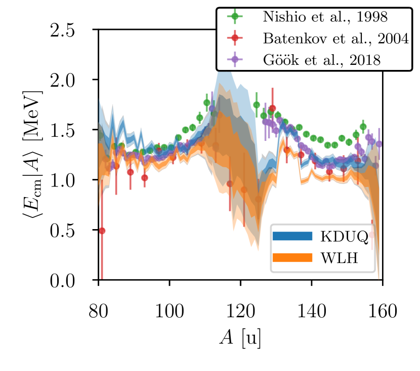
(b) ²³⁵U$(n_{\rm{th}},f)$

Figure 7: Average neutron energy in the COM frame emitted from fragments of a given mass number for (a) ²⁵²Cf$(sf)$, compared to experimental results from Bowman et al. (1963); Göök et al. (2014); Budtz-Jørgensen and Knitter (1988), and (b) ²³⁵U$(n_{\rm{th}},f)$ Nishio et al. (1998); Batenkov et al. (2005); Göök et al. (2018).

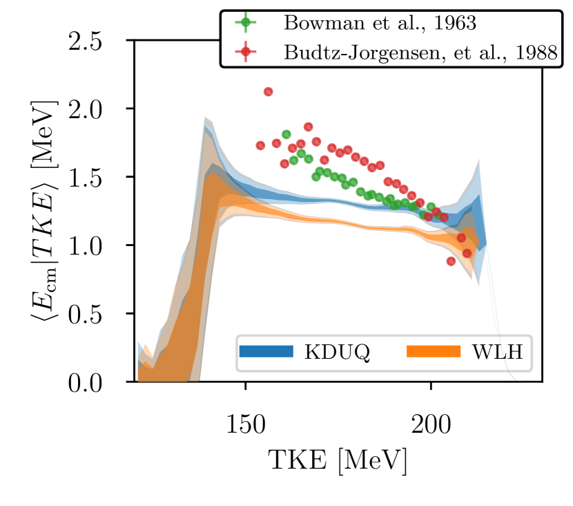
(a) ²⁵²Cf$(sf)$

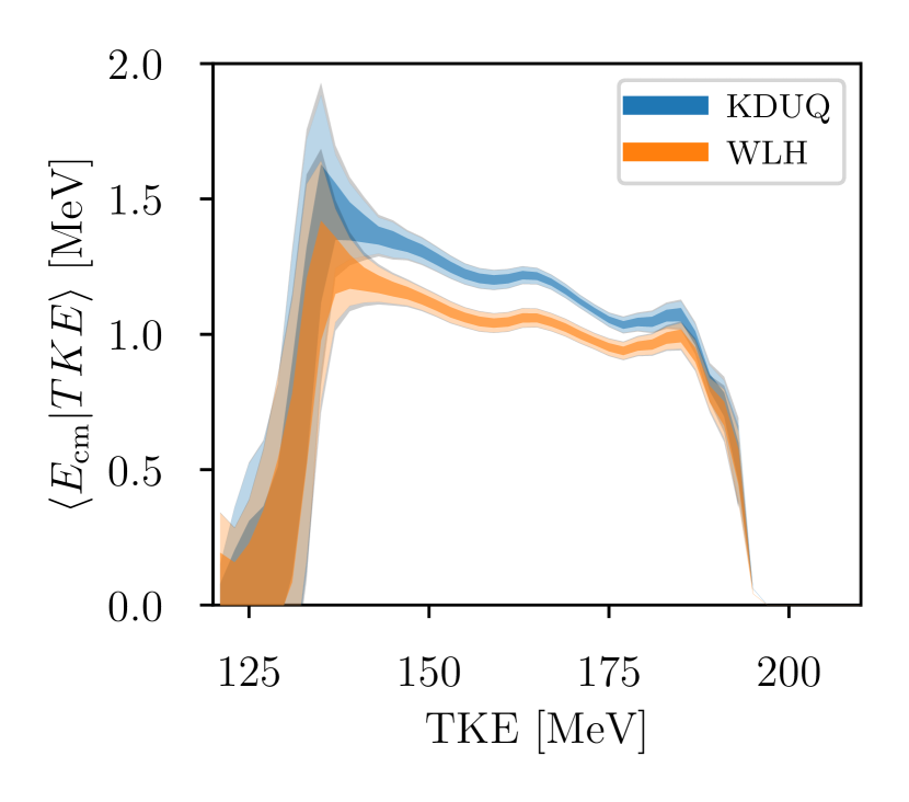
(b) ²³⁵U$(n_{\rm{th}},f)$

Figure 8: Average neutron energy in the COM frame, as a function of the TKE of the fragment pair, for (a) ²⁵²Cf$(sf)$ compared to experimental results from Bowman et al. (1963); Budtz-Jørgensen and Knitter (1988), and (b). ²³⁵U$(n_{\rm{th}},f)$

We now turn our attention to observables relating to the correlation between fragment mass/TKE and mean neutron energy. These experimental comparisons typically required kinematic correction for COM-frame PFNS. In particular, as described in Göök et al. (2014), only neutrons with lab-frame energy larger than the pre-emission kinetic energy per nucleon of the emitting fragment were measured. For comparison to this experiment, these cuts were applied event by event to the generated histories. A similar cut to compare to data from Bowman et al. (1963) was determined to have a negligible effect when applied to CGMF histories, and was subsequently ignored. Additionally, mass reconstruction in the relevant experiments has an uncertainty with a standard deviation of roughly 2-4 mass units.

Figure 7 displays the mean neutron energy as a function of fragment mass. Of course, both models predict spectra that are too soft, however this is not the case uniformly across mass number; the mass dependent behavior of each OMP is different. Interestingly, in the symmetric fission region, the sensitivity of the mean neutron energy was pronounced for ²³⁵U, but not for ²⁵²Cf. In fact, in the respective symmetric fission regions, both models strongly disagree with experiment for ²⁵²Cf, but agree fairly well (despite large uncertainties) for ²³⁵U. Both models exhibit poor agreement, for both fissioning isotopes, in the mass region $125<A<135$, which produces fragments near the ¹³²Sn double shell closure. This indicates a potentially rich mass region to investigate with fission arm spectrometer experiments (e.g. SPIDER Meierbachtol et al. (2015)), for several reasons: 1) nuclides close to the shell closure are approximately spherical, so there is more validity in applying a spherical optical potential to them as opposed to other fission fragment isotopes; 2) the disagreement with experiment is largest here, but this is unexplained by the OMP uncertainties 3) the two OMPs disagree with each other in this region.

Figure 8 displays the mean neutron energy emitted from individual fragments as a function of the TKE of both fragments. The shape of the mean neutron energy dependence of both models as a function of TKE is essentially the same, just shifted by $\sim 100$ keV. It is worth noting the disagreement obtained with experiment, further investigation into the difference between CGMF predictions and experimental measurements of $\bar{E}(TKE)$ should clarify this issue.

IV.3 Differential prompt neutron-fragment correlations

Finally, we consider these same observable differentiated along neutron energy and TKE. For each observable, we look at a set of selected mass pairs, showing the light fragment in the pair in the left columns of Figs. 9,10,11,12,and 13, and the heavy fragment in the right columns. As the mass resolution typical of these experiments is greater than 1 mass unit, we indicate the mass centroid of the data in each panel as approximate, e.g. by $A\sim 100$.

The mass dependence of the PFNS is explored further in Figs. 9 and  10, where single-fragment COM-frame PFNS, $p(E_{cm}|A)$ , are compared to Göök et al. (2014), for a few selected mass number pairs. The mean and shape disagreement between the OMPs and experiment demonstrate the potential for fragment-neutron correlated time-of-flight measurements to constrain the mass-dependence of OMPs away from stability. Particularly interesting is the peaked structure around $\sim 1$ MeV predicted by WLH, uniformly across fragment masses and fissioning isotopes. This is worth further exploration by comparing the WLH model in the HF formalism to experimental neutron evaporation spectra from other reactions. Is this energy feature a hall mark of WLH across the chart of isotopes or emerge only away from $\beta$-stability?

On the experimental side, these spectra indicate a strong deviation from Maxwellian behavior for some fragments with some experiments having more than 5 times the number of neutrons in the $\sim 10$ MeV bin than the models predict, albeit with large uncertainties. This feature has been investigated before Kawano et al. (2021), but the systematic mass-by-mass calibration of model inputs to neutron spectra has yet to be done. Unfortunately, the large experimental uncertainties for most mass numbers does make this a challenge.

The highly asymmetric mass regions for both isotopes are potentially useful as constraints for the OMPs, as they are sensitive while being in regions that are well covered by experiment, with only moderate uncertainties and disagreements between experiments. We would not recommend fitting any non-OMP model inputs to any observables relating to neutron energy, without also considering the OMP amongst the free parameters, as the sensitivity is universally non-negligible.

Figures 11 and 12 display the mean single-fragment multiplicity conditional upon mass number and TKE of the fragment pair, $\langle\nu|TKE,A\rangle$, for a few selected mass number pairs. We see high degree of sensitivity of $\langle\nu|TKE,A\rangle$ to the OMP in the low TKE symmetric mass region. The experimental data is reproduced well for the most part, with the exception of systematic over/under-estimation for fragment pairs; e.g. $A\sim 104,131$ in ²³⁵U. Both models are essentially identical for these observables.

Figure 13 displays the mean neutron energy conditional upon fragment mass and TKE, $\langle E_{cm}|A,TKE\rangle$. While this observable could in principle be extracted from most of the other similar experiments; e.g. Göök et al. (2014, 2018); Budtz-Jørgensen and Knitter (1988), it is only reported by Bowman et al. Bowman et al. (1963) and only for ²⁵²Cf. As this is the most sensitive observable to the optical model, we recommend further experimental study in this direction. In both experiments, the overall shape as a function of TKE was roughly the same for both models. Although the experimental data points are sparse, the agreement is reasonable with the exception of $A=131$, in which it is off by up to an MeV in the region of TKE $\sim 200$ MeV. This is well outside of the parametric model uncertainty and could potentially provide a useful constraint for calibration.

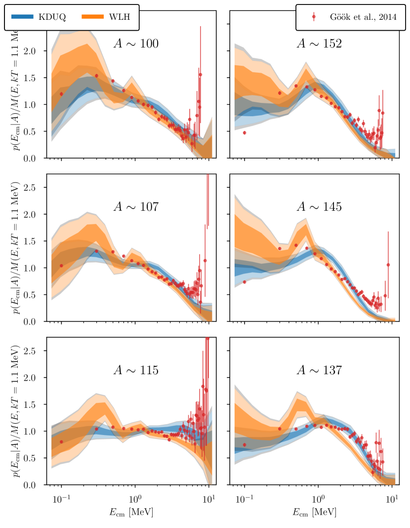
Figure 9: PFNS ratio to a Maxwellian with $kT=1.1$ MeV, conditional on fragment mass, for ²⁵²Cf$(sf)$ compared to experimental data from Göök et al. (2014).

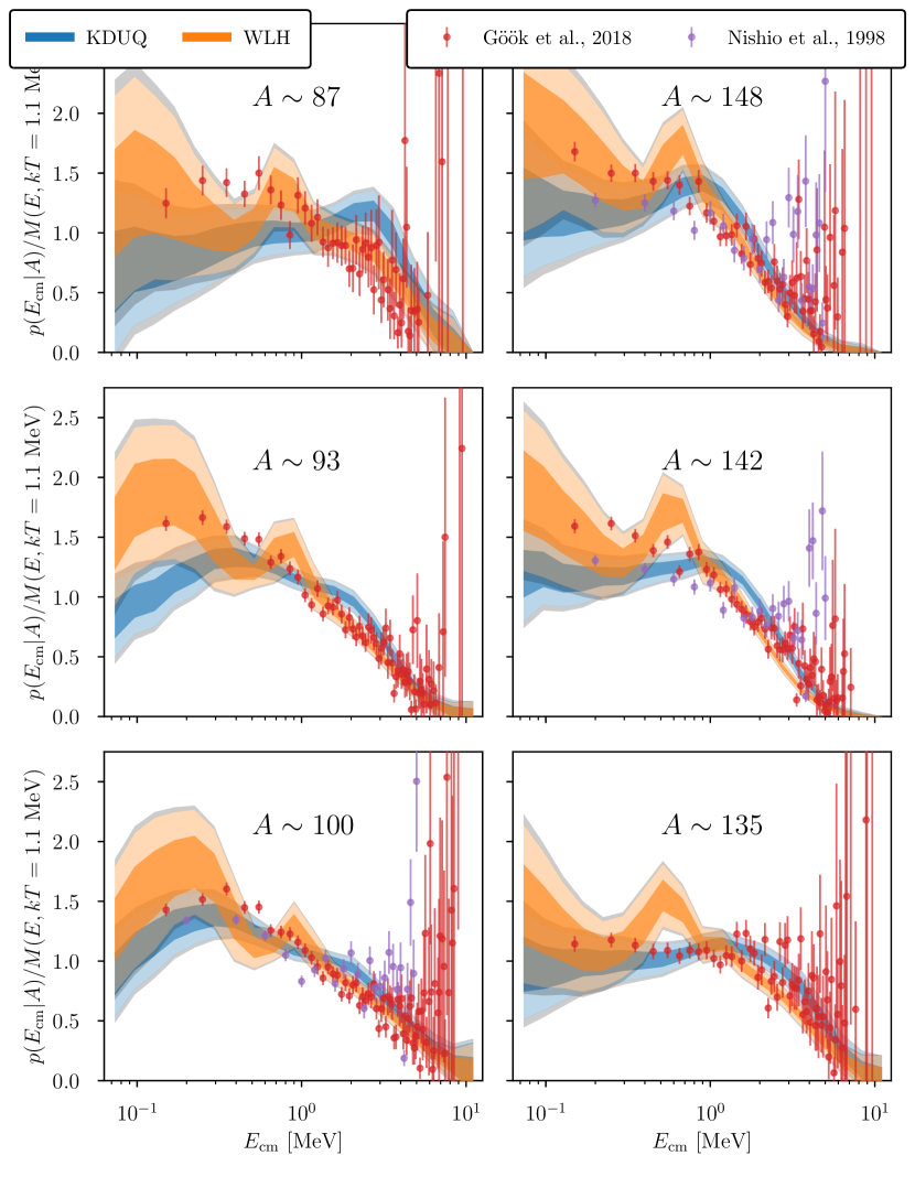
Figure 10: Same as Fig. 3 for ²³⁵U$(n_{th},f)$ compared to experimental data from Göök et al. (2018); Nishio et al. (1998).

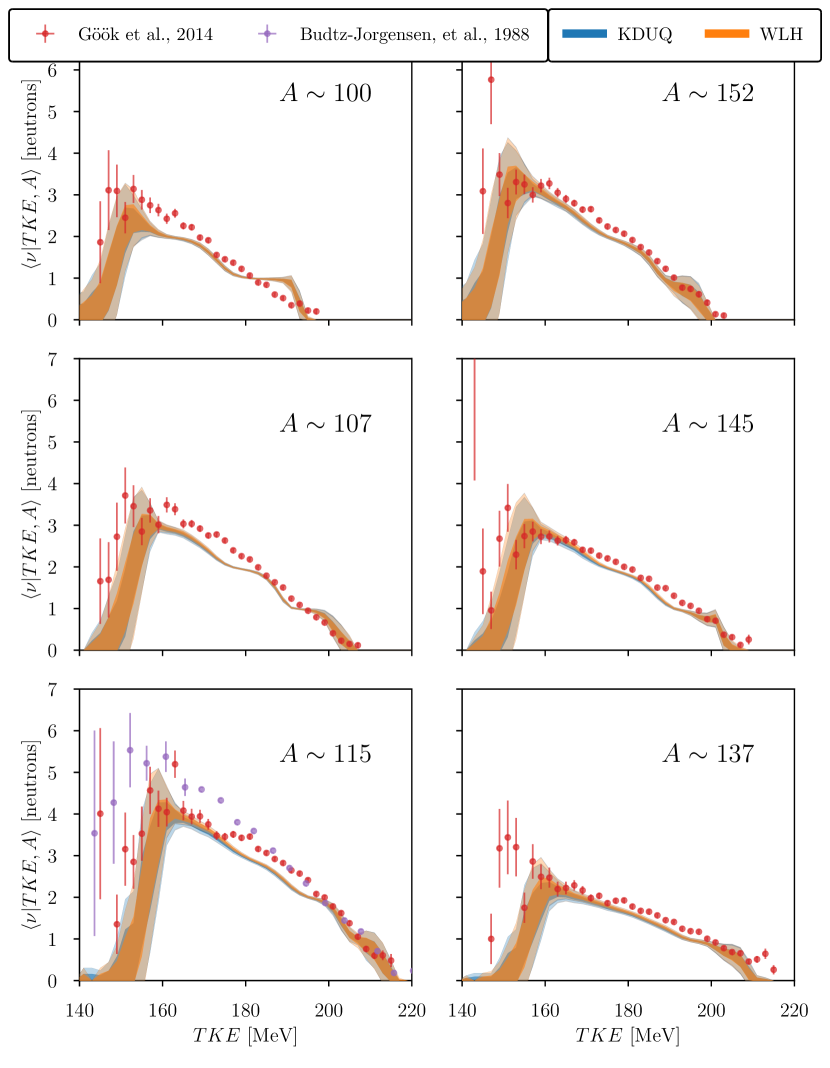
Figure 11: Single-fragment neutron multiplicity as a function of the TKE of both fragments, and conditional on fragment mass, for ²⁵²Cf$(sf)$ compared to experimental data from Göök et al. (2014); Budtz-Jørgensen and Knitter (1988).

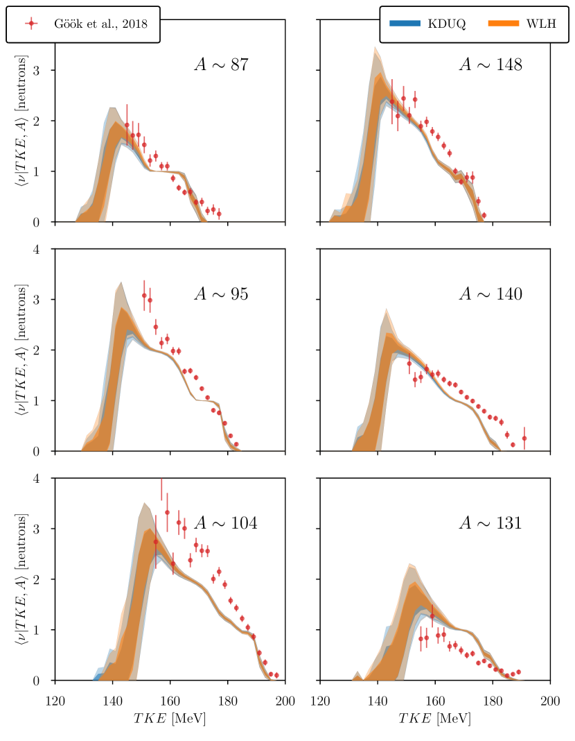
Figure 12: Same as Fig. 11 for ²³⁵U$(n_{th},f)$ compared to experimental data from Göök et al. (2014).

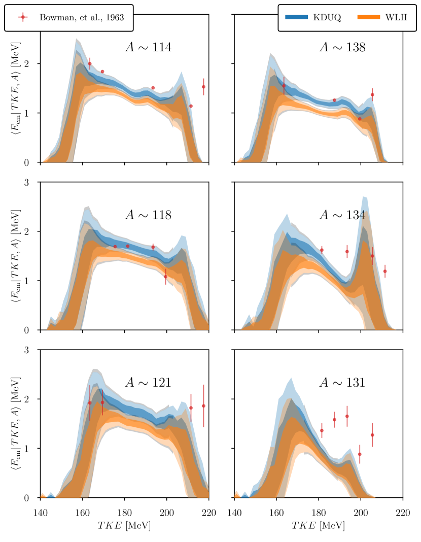
Figure 13: Average COM-frame neutron energy as a function of the TKE of both fragments, and conditional on fragment mass, for ²⁵²Cf$(sf)$ compared to experimental data from Bowman et al. (1963).

V Conclusions

We have shown that neutron-fragment correlated fission observables are sensitive to the form and parameterization of the optical model potential (OMP). In particular, neutron energy spectra are sensitive to OMP form and parameters, especially as a function of total kinetic energy (TKE). Neutron multiplicities are slightly sensitive due to energy budget considerations, but this is a second-order effect and not relevant given the size of experimental uncertainties. On the other hand, neutron energy spectra, when differentiated on mass and TKE, show significant sensitivities to the parameters of individual OMPs, and disagree between the two OMPs themselves. The low TKE region is especially sensitive, although it is difficult to access experimentally.

While the fact that fission observables are sensitive to the parameters and form of the OMP used in the Hauser-Feshbach (HF) de-excitation is encouraging in regard to future efforts to include these observables in OMP calibration, this should be tempered with the fact that many of experimental observables considered here have multiple measurements reported in the literature which disagree with each other well outside of their reported uncertainties. Any future calibration effort will require great care in selecting the evidence used from the available experiments, and in constructing a likelihood model that incorporates the unreported systematic uncertainty.

Of particular interest to future calibration is the energy spectra of neutrons emitted in the mass region near the ¹³²Sn shell closure. The strong disagreement between experiment and theory cannot be explained purely by the uncertainty in the OMP priors, and, furthermore, the OMP forms disagree with each other in this region to statistical significance. Further study of fission fragment initial conditions, informed by experiment, microscopic time-dependent, or adiabatic mean-field calculations of scission, may shed light on the role of excitation energy sharing in this region, but the role of the OMPs cannot be ruled out. Additionally, the parameterization of level densities may need to be revisited. Future work should investigate the sensitivity of these fission observables to level density parameters, as well as fission-fragment initial conditions.

Throughout the observables investigated here, significant differences were observed between OMP forms. The WLH potential in particular predicted much softer spectra overall, and specifically for the heavy fragments than the phenomenological potential, while both produced reasonable spectra for light fragments. This points to potential issues with the nuclear matter folding approach at low energy, due to finite size effects and long-range correlations. This has been pointed out in relation to the JLMB semi-microscopic potential as well Goriely and Delaroche (2007). In general, the imaginary strength of microscopic OMPs developed in folding approaches is smaller than that in corresponding phenomenological potentials, likely due to missing configurations that describe, or act as doorway states to, collective excitations which contribute to compound states. For example, at second order in many-body perturbation theory, 3-particle–2-hole states are neglected. Specifically for the WLH potential, the total imaginary part of the potential is less surface peaked than in phenomenological potentials Holt and Whitehead (2022).

Especially in the case of fission fragments, we expect low-lying collective excitations to arise in the form of rotational and vibrational modes. Explicitly including these couplings in the form of a coupled-channels OMP would, in principle, provide a better description, but this has not been done in the case of fission due to computational constraints and lack of information about excited states in neutron-rich nuclei. However, as described in Sec. II, the HF approach only requires that the branching ratios, not transmission coefficients, to the ground state well describe those to excited states, which alleviates part of this issue.

Future work will explore the possibility of describing deformed fragments by including coupling to low-lying collective excitations. As this is not likely to be computationally tractable within MCHF, emulators capable of significant speed up to the calculation of transmission coefficients are being explored and developed Bonilla et al. (2022); Giuliani et al. (2021); Melendez et al. (2022). Additionally, leveraging microscopic descriptions of excited states is worth exploring if they provide predictions different from collective models or remove poorly constrained input parameters (such as quadrupole deformations of fission fragment ground states) from the calibration.

With regards to the effort towards including fission observables as constraints for OMP parameters; as discussed, there are a wide variety of other fissioning isotopes that can be studied, with a large quantity of associated experimental data. In particular, precision fragment-neutron correlated experiments using time-of-flight fission arm spectrometers promise the most precise fission-fragment measurements to date Meierbachtol et al. (2015). Performing these measurements in correlation with prompt neutrons would likely provide the most precise and detailed data, against which to compare fission models, to date. The ability to leverage emulators to do rapid uncertainty quantification of MCHF models for fission – and other CN processes – would open up the door for adding new constrains to OMPs away from stability.

Future work optimizing model inputs to MCHF fission event generators should be guided by this work to include neutron-fragment correlated multiplicities (i.e. $\bar{\nu}$ conditional on $A$ and/or TKE). Furthermore, measurements of mass-dependent neutron energy spectra provide a (admittedly model-dependent) measurement of fragment temperatures Budtz-Jørgensen and Knitter (1988). Using these as Bayesian priors in such a calibration, or incorporating them as a constraint in the likelihood function, should be investigated.

VI Acknowledgements

The authors would like to thank Stefano Marin for useful discussions about fission fragments and neutron evaporation, and Aaron Tumulak for discussions about Monte Carlo estimators.

This work was funded by the Consortium for Monitoring, Technology, and Verification under Department of Energy National Nuclear Security Administration award number DE-NA0003920, performed under the auspices of the U.S. Department of Energy by Los Alamos National Laboratory under Contract 89233218CNA000001 and under the auspices of the U.S. Department of Energy by Lawrence Livermore National Laboratory under Contract DE-AC52-07NA27344. This work was also supported by the Laboratory Directed Research and Development program of Los Alamos National Laboratory under project number 20220532ECR.

Appendix A Uncertainty propagation with Monte Carlo

The spread of the mean in each observable over all parameter samples reflects the sum of two uncertainties: the intrinsic parametric uncertainty of each OMP, and the inherent uncertainty due to the limited number of Monte Carlo histories per parameter sample. These uncertainties are assumed to be uncorrelated, so that the total uncertainty $\sigma_{t}$ across the ensemble of OMP samples was taken as the quadrature sum of the MCHF uncertainty and the parametric uncertainty of the OMP. The latter was estimated as

$$\sigma_{omp}=\sqrt{\sigma_{t}^{2}-\sigma_{mc}^{2}}.$$ (8)

For a given ensemble of histories corresponding to OMP parameter sample $i$, a Monte Carlo uncertainty $\sigma^{i}_{mc}$ was calculated for each observable. For observables that correspond to the mean of a distribution over events (e.g. average prompt neutron multiplicity $\bar{\nu}$), $\sigma^{i}_{mc}$ corresponded to the standard error in the mean (SEM), and was estimated directly from the second moment of the distribution of the observable over all histories in the ensemble:

$$\sigma^{i}_{mc}=\sqrt{\frac{1}{N}\sum_{n}(k^{i}_{n})^{2}-\frac{1}{N^{2}}\left(\sum_{n}k^{i}_{n}\right)^{2}},$$ (9)

where $k^{i}_{n}$ represents the score for the observable of interest in the $n^{\rm{th}}$ (out of $N$) histories of the $i^{\rm{th}}$ sample.

Observables corresponding to distributions (e.g. PFNS), were constructed by histogramming over ensemble histories, in which case the mean of an observable in a bin corresponded to the probability density of $k^{i}_{n}$ falling into that bin in a given history. For $m$ times out of $N$ histories in a bin in phase space with width $\Delta x$, the mean is $m/(N\Delta x)$. In this case, $\sigma^{i}_{mc}$ was estimated in each histogram bin according to a Binomial distribution:

$$\sigma^{i}_{mc}=\frac{1}{N\Delta X}\sqrt{1-\frac{m}{N}}.$$ (10)

In either case, $\sigma_{mc}$ for the observable was then estimated by averaging $\sigma^{i}_{mc}$ over all ensembles.

References

- Hebborn et al. (2022a) C. Hebborn, G. Hupin, K. Kravvaris, S. Quaglioni, P. Navrátil, and P. Gysbers, Phys. Rev. Lett. 129, 5 (2022a).
- for the Horizon: The 2015 Long Range Plan for Nuclear Science (2015) R. for the Horizon: The 2015 Long Range Plan for Nuclear Science, (2015).
- Trkov et al. (2015) A. Trkov, R. Capote, and V. Pronyaev, Nuclear Data Sheets 123, 8 (2015).
- Capote et al. (2016) R. Capote, Y.-J. Chen, F.-J. Hambsch, N. Kornilov, J. Lestone, O. Litaize, B. Morillon, D. Neudecker, S. Oberstedt, T. Ohsawa, et al., Nuclear Data Sheets 131, 1 (2016).
- Lovell and Neudecker (2021) A. E. Lovell and D. Neudecker, Correcting the PFNS for more consistent fission modeling, Tech. Rep. (Los Alamos National Lab.(LANL), Los Alamos, NM (United States), 2021).
- Lovell and Neudecker (2022) A. E. Lovell and D. Neudecker, Energy-dependent optimization of the prompt fission neutron spectrum with CGMF, Tech. Rep. (Los Alamos National Lab.(LANL), Los Alamos, NM (United States), 2022).
- Talou et al. (2021) P. Talou, I. Stetcu, P. Jaffke, M. E. Rising, A. E. Lovell, and T. Kawano, Computer Physics Communications 269, 108087 (2021).
- Koning and Delaroche (2003) A. Koning and J. Delaroche, Nuclear Physics A 713, 231 (2003).
- Moldauer (1962) P. Moldauer, Physical Review Letters 9, 17 (1962).
- Goriely and Delaroche (2007) S. Goriely and J.-P. Delaroche, Physics Letters B 653, 178 (2007).
- Xu et al. (2010) C. Xu, B.-A. Li, and L.-W. Chen, Phys. Rev. C 82, 054607 (2010).
- Bollen (2010) G. Bollen, in AIP Conference Proceedings, Vol. 1224 (American Institute of Physics, 2010) pp. 432–441.
- Lovell and Nunes (2018) A. E. Lovell and F. M. Nunes, Phys. Rev. C 97, 064612 (2018).
- King et al. (2019) G. B. King, A. E. Lovell, L. Neufcourt, and F. M. Nunes, Phys. Rev. Lett. 122, 232502 (2019).
- Catacora-Rios et al. (2019) M. Catacora-Rios, G. B. King, A. E. Lovell, and F. M. Nunes, Phys. Rev. C 100, 064615 (2019).
- Lovell et al. (2020) A. Lovell, F. M. Nunes, M. Catacora-Rios, and G. King, Journal of Physics G: Nuclear and Particle Physics 48, 014001 (2020).
- Catacora-Rios et al. (2021) M. Catacora-Rios, G. King, A. E. Lovell, and F. M. Nunes, Physical Review C 104, 064611 (2021).
- Pruitt et al. (2023) C. Pruitt, J. Escher, and R. Rahman, Physical Review C 107, 014602 (2023).
- Whitehead et al. (2022) T. Whitehead, T. Poxon-Pearson, F. Nunes, and G. Potel, Physical Review C 105, 054611 (2022).
- Hebborn et al. (2022b) C. Hebborn, T. Whitehead, A. E. Lovell, and F. M. Nunes, arXiv preprint arXiv:2212.06056 (2022b).
- Smith et al. (2024) A. Smith, C. Hebborn, F. Nunes, and R. Zegers, arXiv preprint arXiv:2403.18629 (2024).
- Kawano et al. (2021) T. Kawano, S. Okumura, A. E. Lovell, I. Stetcu, and P. Talou, Phys. Rev. C 104, 014611 (2021).
- Voinov et al. (2007) A. Voinov, S. Grimes, C. Brune, M. Hornish, T. Massey, and A. Salas, Physical Review C 76, 044602 (2007).
- Wallner et al. (1995) A. Wallner, B. Strohmaier, and H. Vonach, Physical Review C 51, 614 (1995).
- Ramirez et al. (2013) A. Ramirez, A. Voinov, S. Grimes, A. Schiller, C. Brune, T. Massey, and A. Salas-Bacci, Physical Review C 88, 064324 (2013).
- Talou and Vogt (2023) P. Talou and R. Vogt, Nuclear Fission: Theories, Experiments and Applications (Springer Nature, 2023).
- Schunck and Regnier (2022) N. Schunck and D. Regnier, Progress in Particle and Nuclear Physics 125, 103963 (2022).
- Schmitt et al. (1965) H. Schmitt, W. Kiker, and C. Williams, Physical Review 137, B837 (1965).
- Marin et al. (2020) S. Marin, V. A. Protopopescu, R. Vogt, M. J. Marcath, S. Okar, M. Y. Hua, P. Talou, P. F. Schuster, S. D. Clarke, and S. A. Pozzi, Nuclear Instruments and Methods in Physics Research Section A: Accelerators, Spectrometers, Detectors and Associated Equipment 968, 163907 (2020).
- Oberstedt et al. (2013) A. Oberstedt, T. Belgya, R. Billnert, R. Borcea, T. Bryś, W. Geerts, A. Göök, F.-J. Hambsch, Z. Kis, T. Martinez, et al., Physical Review C 87, 051602 (2013).
- Wilson et al. (2021) J. Wilson, D. Thisse, M. Lebois, N. Jovančević, D. Gjestvang, R. Canavan, M. Rudigier, D. Étasse, R. Gerst, L. Gaudefroy, et al., Nature 590, 566 (2021).
- Hoffman (1964) M. M. Hoffman, Physical Review 133, B714 (1964).
- Franklyn et al. (1978) C. Franklyn, C. Hofmeyer, and D. Mingay, Physics Letters B 78, 564 (1978).
- Budtz-Jørgensen and Knitter (1988) C. Budtz-Jørgensen and H.-H. Knitter, Nuclear Physics A 490, 307 (1988).
- Stetcu et al. (2021) I. Stetcu, A. E. Lovell, P. Talou, T. Kawano, S. Marin, S. A. Pozzi, and A. Bulgac, Physical Review Letters 127, 222502 (2021).
- Thompson and Nunes (2009) I. J. Thompson and F. M. Nunes, Nuclear reactions for astrophysics: principles, calculation and applications of low-energy reactions (Cambridge University Press, 2009).
- Hauser and Feshbach (1952) W. Hauser and H. Feshbach, Physical review 87, 366 (1952).
- Satchler (1963) G. Satchler, Physics Letters 7, 55 (1963).
- Whitehead et al. (2021) T. Whitehead, Y. Lim, and J. Holt, Physical Review Letters 127, 182502 (2021).
- Lim and Holt (2017) Y. Lim and J. W. Holt, Phys. Rev. C 95, 065805 (2017).
- Holt et al. (2011) J. Holt, N. Kaiser, and W. Weise, The European Physical Journal A 47, 1 (2011).
- Wahl (1980) A. Wahl, Journal of Radioanalytical Chemistry 55, 111 (1980).
- Kawano et al. (2006) T. Kawano, S. Chiba, and H. Koura, Journal of Nuclear Science and Technology 43, 1 (2006), https://www.tandfonline.com/doi/pdf/10.1080/18811248.2006.9711062 .
- Forum (1994) M. P. Forum, MPI: A Message-Passing Interface Standard, Tech. Rep. (USA, 1994).
- Dalcín et al. (2005) L. Dalcín, R. Paz, and M. Storti, Journal of Parallel and Distributed Computing 65, 1108 (2005).
- (46) K. Beyer, “Osiris,” .
- Krekel et al. (2004) H. Krekel, B. Oliveira, R. Pfannschmidt, F. Bruynooghe, B. Laugher, and F. Bruhin, “pytest 8.2,” (2004).
- Hořeňovský (2024) M. Hořeňovský, “Catch2 3.5,” (2024).
- Croft et al. (2020) S. Croft, A. Favalli, and R. D. McElroy Jr., Nuclear Instruments and Methods in Physics Research Section A: Accelerators, Spectrometers, Detectors and Associated Equipment 954, 161605 (2020), symposium on Radiation Measurements and Applications XVII.
- Brown et al. (2018) D. A. Brown, M. Chadwick, R. Capote, A. Kahler, A. Trkov, M. Herman, A. Sonzogni, Y. Danon, A. Carlson, M. Dunn, et al., Nuclear Data Sheets 148, 1 (2018).
- Santi and Miller (2008) P. Santi and M. Miller, Nuclear Science and Engineering 160, 190 (2008), https://www.tandfonline.com/doi/pdf/10.13182/NSE07-85 .
- Vorobyev et al. (2010) A. Vorobyev, O. Shcherbakov, Y. S. Pleve, A. Gagarski, G. Val’ski, G. Petrov, V. Petrova, T. Zavarukhina, I. Guseva, V. Sokolov, et al., in Proc. of the XVII International Seminar on Interaction of Neutrons with Nuclei: Neutron Spectroscopy, Nuclear Structure, Related Topics (AM Sukhovoj, ed.),(Dubna) (2010) p. 60.
- Dushin et al. (2004) V. Dushin, F.-J. Hambsch, V. Jakovlev, V. Kalinin, I. Kraev, A. Laptev, D. Nikolaev, B. Petrov, G. Petrov, V. Petrova, Y. Pleva, O. Shcherbakov, V. Shpakov, V. Sokolov, A. Vorobyev, and T. Zavarukhina, Nuclear Instruments and Methods in Physics Research Section A: Accelerators, Spectrometers, Detectors and Associated Equipment 516, 539 (2004).
- Vorobyev (2001) A. Vorobyev, in International Seminar on Interactions of Neutrons with Nuclei,(ISINN-9), 2001, Vol. 9 (2001) pp. 276–295.
- Spencer et al. (1982) R. R. Spencer, R. Gwin, and R. Ingle, Nuclear Science and Engineering 80, 603 (1982), https://doi.org/10.13182/NSE82-A18973 .
- Edwards et al. (1982) G. Edwards, D. Findlay, and E. Lees, Annals of Nuclear Energy 9, 127 (1982).
- Gwin et al. (1984) R. Gwin, R. Spencer, and R. Ingle, Nuclear Science and Engineering 87, 381 (1984).
- Holden and Zucker (1988) N. E. Holden and M. S. Zucker, Nuclear Science and Engineering 98, 174 (1988).
- Boldeman and Hines (1985) J. W. Boldeman and M. G. Hines, Nuclear Science and Engineering 91, 114 (1985), https://doi.org/10.13182/NSE85-A17133 .
- Carlson et al. (2009) A. Carlson, V. Pronyaev, D. Smith, N. M. Larson, Z. Chen, G. Hale, F.-J. Hambsch, E. Gai, S.-Y. Oh, S. Badikov, et al., Nuclear Data Sheets 110, 3215 (2009).
- Kikuchi et al. (1977) Y. Kikuchi, T. Nakagawa, H. Matsunobu, Y. Kanda, and M. Kawai, (1977).
- Märten et al. (1990) H. Märten, D. Richter, D. Seeliger, W. Fromm, R. Böttger, and H. Klein, Nuclear science and engineering 106, 353 (1990).
- Nefedov (1983) V. Nefedov, in All-Union Conf. Neutron Physics, Kiev, Oct. 2-6, 1983, Vol. 2 (1983) p. 285.
- Lajtai et al. (1990) A. Lajtai, P. Dyachenko, V. Kononov, and E. Seregina, Nuclear Instruments and Methods in Physics Research Section A: Accelerators, Spectrometers, Detectors and Associated Equipment 293, 555 (1990).
- Kornilov (2015) N. Kornilov, INDC (USA)-108, International Atomic Energy Agency, International Nuclear Data Committee (2015).
- Werle and Bluhm (1972) H. Werle and H. Bluhm, Journal of Nuclear Energy 26, 165 (1972).
- Chalupka et al. (1990) A. Chalupka, L. Malek, S. Tagesen, and R. Böttger, Nuclear Science and Engineering 106, 367 (1990).
- Coelho et al. (1989) P. R. Coelho, A. A. Da Silva, and J. R. Maiorino, Nuclear Instruments and Methods in Physics Research Section A: Accelerators, Spectrometers, Detectors and Associated Equipment 280, 270 (1989).
- Starostov et al. (1983) B. Starostov, V. Nefedov, and A. Boytzov, in Nejtronnaja Fizika (6-th Conf. for Neutron Phys., Kiev. 1983), v2. p285, Vol. 290 (1983) p. 294.
- Lajtai et al. (1986) A. Lajtai, J. Kecskeméti, J. Sáfár, P. Dyachenko, and V. Piksaikin, Radiation Effects 93, 277 (1986).
- Yufeng et al. (1992) W. Yufeng, B. Xixiang, L. Anli, W. Xiaozhong, L. Jingwen, M. Jiangchen, and B. Zongyu, in Physics and Chemistry of Fission: Proceedings of the XVIIIth International Symposium on Nuclear Physics, Gaussig (GDR), 21-25 November 1988 (Nova Publishers, 1992) p. 183.
- Göök et al. (2014) A. Göök, F.-J. Hambsch, and M. Vidali, Phys. Rev. C 90, 064611 (2014).
- Zeynalov et al. (2009) S. Zeynalov, F.-J. Hambsch, S. Oberstedt, and I. Fabry, in AIP Conference Proceedings, Vol. 1175 (American Institute of Physics, 2009) pp. 359–362.
- Bowman et al. (1963) H. R. Bowman, J. Milton, S. G. Thompson, and W. J. Swiatecki, Physical Review 129, 2133 (1963).
- Ding et al. (1984) S. Ding, J. Xu, Z. Liu, Q. Zhang, S. Liu, and H. Zhang, Chinese Journal of Nuclear Physics 6, 201 (1984).
- Batenkov et al. (2005) O. Batenkov, G. Boykov, F.-J. Hambsch, J. Hamilton, V. Jakovlev, V. Kalinin, A. Laptev, V. Sokolov, and A. Vorobyev, in AIP Conference Proceedings, Vol. 769 (American Institute of Physics, 2005) pp. 1003–1006.
- Nishio et al. (1998) K. Nishio, Y. Nakagome, H. Yamamoto, and I. Kimura, Nuclear Physics A 632, 540 (1998).
- Göök et al. (2018) A. Göök, F.-J. Hambsch, S. Oberstedt, and M. Vidali, Physical Review C 98, 044615 (2018).
- Boldeman et al. (1971) J. Boldeman, A. de L Musgrove, and R. Walsh, Australian Journal of Physics 24, 821 (1971).
- Meierbachtol et al. (2015) K. Meierbachtol, F. Tovesson, D. Shields, C. Arnold, R. Blakeley, T. Bredeweg, M. Devlin, A. Hecht, L. Heffern, J. Jorgenson, et al., Nuclear Instruments and Methods in Physics Research Section A: Accelerators, Spectrometers, Detectors and Associated Equipment 788, 59 (2015).
- Holt and Whitehead (2022) J. W. Holt and T. R. Whitehead, in Handbook of Nuclear Physics (Springer, 2022) pp. 1–30.
- Bonilla et al. (2022) E. Bonilla, P. Giuliani, K. Godbey, and D. Lee, Physical Review C 106, 054322 (2022).
- Giuliani et al. (2021) P. Giuliani, C. Drischler, A. Lovell, M. Quinonez, and F. Nunes, in APS Division of Nuclear Physics Meeting Abstracts, Vol. 2021 (2021) pp. LM–006.
- Melendez et al. (2022) J. Melendez, C. Drischler, R. Furnstahl, A. Garcia, and X. Zhang, Journal of Physics G: Nuclear and Particle Physics 49, 102001 (2022).