11email: {sotasato,jiean,hasuo}@nii.ac.jp 22institutetext: Kyushu University, Fukuoka, Japan
22email: zhang@ait.kyushu-u.ac.jp 33institutetext: SOKENDAI (The Graduate University for Advanced Studies), Tokyo, Japan 44institutetext: Institute of Software, Chinese Academy of Sciences, Beijing, China
Optimization-Based Model Checking and
Trace Synthesis for Complex STL Specifications
(Extended Version)††thanks: The authors are supported by ERATO HASUO Metamathematics for Systems
Design Project (No. JPMJER1603), the START Grant No. JPMJST2213, the ASPIRE grant No. JPMJAP2301, JST. S.S. is supported by KAKENHI No. 23KJ1011, JSPS. Z.Z. is supported by JSPS KAKENHI Grant No. JP23K16865 and No. JP23H03372.
Abstract
Techniques of light-weight formal methods, such as monitoring and falsification, are attracting attention for quality assurance of cyber-physical systems. The techniques require formal specs, however, and writing right specs is still a practical challenge. Commonly one relies on trace synthesis—i.e. automatic generation of a signal that satisfies a given spec—to examine the meaning of a spec. In this work, motivated by 1) complex STL specs from an automotive safety standard and 2) the struggle of existing tools in their trace synthesis, we introduce a novel trace synthesis algorithm for STL specs. It combines the use of MILP (inspired by works on controller synthesis) and a variable-interval encoding of STL semantics (previously studied for SMT-based STL model checking). The algorithm solves model checking, too, as the dual of trace synthesis. Our experiments show that only ours has realistic performance needed for the interactive examination of STL specs by trace synthesis.
1 Introduction
Safety and quality assurance of cyber-physical systems (CPSs) is an important and multifaceted problem. The pervasiveness and safety-critical nature of CPSs makes the problem imminent and pressing; at the same time, the problem comes with very different flavors in different application domains, calling for different solutions. For example, in the aerospace domain, full formal verification all the way up from the codebase seems feasible [35]. Such is a luxury that the automotive domain may not afford, however, because of short product cycles, dependence on third-party (thus black-box) components, heterogeneous environmental uncertainties, and fierce competition (thus tight budget).
The above limitations in the automotive domain point, in the formal methods terms, to the absence of white-box system models. This has led to the flourish of light-weight formal methods, such as monitoring [8], runtime verification, and hybrid system falsification [16]. These are logic-based methods that operate on formal specifications, often given in signal temporal logic (STL) [26]. These methods give up comprehensive guarantee due to the absence of white-box system models; yet their values in practical usage scenarios are widely acknowledged.
Trace Synthesis and Model Checking. In this paper, we are motivated by some automotive instances of the trace synthesis problem: it asks to synthesize an execution trace of a system that satisfies a given STL specification . There are two major approaches to trace synthesis for CPSs.
One common approach is via hybrid system falsification [16]: here, we try many input signals for , iteratively modifying them in the direction of satisfying ; the quantitative robust semantics of STL [17] serves as an objective function that allows hill-climbing optimization. It is notable that the system model can be black-box: we do not need to know its internal working; it is enough to compute the execution trace under given input . Falsification has attracted a lot of interest especially in the automotive domain; see e.g. [16].
We take the other approach to trace synthesis, namely as the dual of the model checking problem. Here model checking decides if, under any input , the execution trace satisfies . Our choice of this approach may be puzzling—it requires a white-box model , but it is rare in the automotive domain.
Analyzing Specifications (Rather Than Models). Our choice of the model checking approach to trace synthesis comes from the following basic scope of the paper: we use trace synthesis to analyze the quality of specifications (specs).
This is in stark contrast with many falsification tools whose scope is analyzing models. There, a model is extensive and complex (typically a Simulink model of an actual product), and counterexample traces are used for “debugging” .
In this paper, instead, a model is simple and white-box (it can even be the trivial model, where the input and output are the same), but a spec tends to be complex. One typical usage scenario for our framework is when is a normative rule—such as a law, a traffic rule, or a property required in an international standard—in which case is imposed on many different systems (e.g. different vehicle models). Then should be a simple overapproximation of a variety of systems, rather than a detailed system model.
Another typical usage scenario of our framework is an early “requirement development” phase of the V-model of the automotive system design. Here, engineers fix specs that pin down the later development efforts, in which those specs get refined and realized. They want to confirm that the specs are sensible (e.g. there is no mutual conflict) and faithful to their intentions. Since a system is yet to be developed, a system model cannot be detailed.
Motivating Example. More specifically, the current work is motivated by the work [32] on formalizing disturbance scenarios in the ISO 34502 standard for automated driving vehicles. There, a vehicle dynamics model is simple (the scenarios should apply to different vehicle models—see above), but STL formulas are complex. It is observed that existing algorithms have a hard time handling the complexity of specs (see Section 6 for experiments). This motivated our current technical development, namely a trace synthesis algorithm that exploits white-box models and MILP optimization for efficiency.
The following example illustrates the challenge encountered in [32].

Example 1.1 (rear-end near collision)
We would like to express, in STL, a rear-end near collision scenario for two cars. It refers to those driving situations where a rear car comes too close to a front car . We assume a single-lane setting (Fig. 1), so we can ignore lateral dynamics.
Consider the following STL formulas. Here, are the variables for the position, velocity, and acceleration of ; the other variables are for .
| (5) |
The last formula formalizes rear-end near collision; in particular, its subformula requires that occurs within 9 seconds and persists for at least one second.
The formula comes with two auxiliary conditions: and . We shall now exhibit their content and why they are needed. In fact, these conditions arose naturally in the course of trace synthesis, the problem of our focus.
Specifically, in [32], we conducted trace synthesis repeatedly in order to 1) illustrate the meaning of STL specifications and 2) confirm that they reflect informal intentions. The generated traces were animated for graphical illustration. This workflow is much like in the tool STLInspector [33].
The formula imposes basic constraints on the dynamics of the cars. In the trace synthesis in [32], without this basic constraint, we obtained a number of nonsensical example traces in which a car warps and instantly passes the other, drives much faster than the legal maximum, and so on.
The formula requires to accelerate until occurs. It was added to limit a generated trace to an interesting part. For example, a trace can have only after a -second pacific journey; animating this whole trace can easily bore users. The condition trims such a trace to the part where is accelerating towards .
Remark 1.2
In [32], after illustrating and confirming STL specs through trace synthesis, the final goal was to use them for monitoring actual driving data. Neither the dynamics model 6 nor the condition is really relevant to monitoring—actual driving data should comply with them anyway. In contrast, is important, in order to extract only relevant parts of the data.
Technical Solution: MILP-Based Trace Synthesis. We present a novel trace synthesis algorithm. Note that it also solves the dual problem, namely STL model checking. It originates from two recent lines of work: MILP-based optimal control [31, 30, 14] and SMT-based STL model checking [7, 25, 37].
The controller synthesis techniques in [31, 30, 14] exploit mixed-integer linear programming (MILP) for efficiency. The optimal control problem that they solve can be specialized to our trace synthesis problem (detailed discussions come later). But we found their capability of handling complex specs (as in Thm. 1.1) limited, largely because of their constant-interval encoding to MILP.
We solve this challenge by our novel variable-interval encoding of the STL semantics to MILP. It is inspired by the stable partitioning technique introduced in [7]: the technique is used in [7, 25, 37] for logical encoding towards SMT-based model checking; we use it for numerical encoding to MILP. This way we will solve the bounded trace synthesis problem—in the sense that variability of the truth values of the relevant formulas is bounded—much like in [7, 25, 37]. For our MILP encoding, however, we need special care since MILP does not accommodate strict inequalities (partitions such as in [7] cannot be expressed). We therefore use a novel technique called -stable partitioning.
Overall, our algorithm works as follows. We assume that a system model can be MILP-encoded, either exactly or approximately. Some model families are discussed in Section 5. This assumption, combined with our key technique of variable-interval MILP encoding of STL, reduces trace synthesis to an MILP problem, which we solve by Gurobi Optimizer [20]. We conduct experimental evaluation to confirm the scalability of our algorithm, especially for complex specs (Section 6).
Our algorithm is anytime (i.e. interruptible): even if the budget runs out in the course of optimization, a best-effort result (the trace that is the closest to a solution so far) is obtained. A similar benefit is there in case there is no execution trace that satisfies the spec : we obtain a trace that is the closest to satisfy . Accommodation of parameters is another advantage thanks to our use of MILP; we exploit it for parameter mining for PSTL formulas. See Section 3.
Both controller synthesis techniques [31, 30, 14] and SMT-based model checking techniques [7, 25, 37] can be used for trace synthesis. The methodological differences are discussed later in Section 1; experimental comparison is made in Section 6.
Contributions and Organization. We summarize our contributions.
-
•
We introduce an optimization-based algorithm for bounded trace synthesis for STL specs. It assumes that a system model is white-box and MILP-encodable; it also solves the dual problem (namely bounded model checking).
-
•
As a key element, we introduce a variable-interval encoding of STL to MILP.
-
•
MILP encodings of some system models, notably rectangular hybrid automata and double integrator dynamics (suited for the automotive domain).
- •
-
•
Through the algorithm, case studies and experiments, we argue for the importance and feasibility of spec analysis for CPSs.
After exhibiting preliminaries on STL and stable partitioning in Section 2, we formulate our problems (bounded trace synthesis, model checking, etc.) in Section 3. In Section 4 we present a novel variable-interval MILP encoding of STL; in Section 5 we discuss MILP encoding of a few families of models. Our main algorithm combines these two encodings. In Section 6 we present experiment results.
Related Work I: Optimal STL Control with MILP. The works [31, 30, 14] inspire our use of MILP for STL. Their problem is optimal controller synthesis under STL constraints, i.e. to find an input signal to a system model so that 1) the output signal satisfies a given STL spec and 2) it optimizes , where is a given objective function. This problem subsumes our problem of trace synthesis, by taking a constant function as .
The algorithms in [31, 30, 14] reduce their problem to MILP by a constant-interval encoding of the robust semantics [13, 17] of STL (an enhanced encoding is presented in [24]). Specifically, their system model is discrete-time dynamics with a constant interval .
In contrast, in our variable-interval encoding (Section 4), continuous time is discretized into the intervals where the end points are also variables in MILP. This is advantageous not only in modeling precision but also in scalability: for system models that are largely continuous, constant-interval discretization incurs more integer variables in MILP, hampering the performance of MILP solvers. See Section 6 for experimental comparison.
Related Work II: SMT-Based STL Model Checking. Our key technical element (a variable-interval MILP encoding of STL) uses the idea of stable partitioning from [7, 25, 37]. They solve bounded STL model checking, and also its dual (trace synthesis). The main difference is the class of system models accommodated. SMT solvers accommodate more theories than MILP solving, and thus allows encoding of a greater class of models. In contrast, by restricting the model class to MILP-encodable, our algorithm benefits speed and scalability (MILP is faster than SMT). Iterative optimization in MILP also makes our algorithm an anytime one. Native support of parameter synthesis is another plus.
Other Related Work. Optimization-based falsification has its root in the quantitative robust semantics of STL [13, 17]; the successful combination with stochastic optimization metaheuristics has made falsification an approach of both scientific and industrial interest. See the ARCH competition report [16] for state-of-the-art. Falsification is most of the time thought of as search-based testing; therefore, unlike the model checking approach, the absence of counterexamples is usually not proved. Exceptions are [27, 38] where they strive for probabilistic guarantees for such absence.
The current work is motivated by the observation that falsification solvers often struggle in trace synthesis for complex STL specs, even if a system model is simple. It is known that specs with more connectives pose a performance challenge, and many countermeasures are proposed, including [2] (for temporal operators) and [40, 39] (for Boolean connectives).
2 Preliminaries
We let denote the sets of natural numbers and reals, respectively; denotes an obvious subset. The set is that of extended reals. The set is for Boolean truth values. The powerset of a set is denoted by . An interval is a subset of of the form , , , or , where and . Therefore a singleton is an interval.
Definition 2.1 (linear predicate and )
Given a set of variables, a (closed) linear predicate is a function defined as follows, using some and : if and only if . We write for the closed half-space .
For the above , we define a function by . This is understood as the degree of satisfaction (or violation, if negative) of a linear predicate by . Indeed, is the (signed) Euclidean distance to the boundary of , assuming that the Euclidean norm of is .
Definition 2.2 (signal)
Let be a finite set of variables and a positive real. A signal over with a time horizon is a function . We write for the set of all signals over with time horizon , or simply when is clear from the context.
If necessary, the domain of can be extended to by setting for all . This allows us to define the notion of -postfix, which will serve as the basis of the STL semantics (Section 2.1). Precisely, the -postfix of is a signal defined by . The domain of can be chosen freely but we set it to for consistency.
Definition 2.3 (system model, trace set )
Let be finite sets of variables. A system model from to with a time horizon is a function . The trace set of a system model is that is, the set of all output signals of where an input signal can vary.
We allow system models to be nondeterministic (note the the powerset construction ); the models in Section 1 were deterministic for simplicity. A special case of the above is when , that is, when does not have any input. In this case, is a singleton, and therefore a function can be identified with a subset .
Example 2.4 ()
The dynamics model in Thm. 1.1 is formalized as a system model whose input variables (in ) are , and output variables (in ) are . Here, the input is acceleration rates () and the initial values of velocities and positions (modeled using signals etc. for convenience). The time horizon of represents its simulation time; here we set . Given an input signal , the output is a singleton , and is determined by the ODE 6. Specifically, , , and so on.
2.1 Signal Temporal Logic
Definition 2.5 (signal temporal logic (STL))
In STL, an atomic proposition over a variable set is represented as , where is a function that maps a -dimensional vector to a real. The syntax of an STL formula (over ) is defined as follows: , where is a nonsingular closed time interval, and , , are temporal operators eventually, always, until and release. Implication is defined: . We write temporal operators without the subscript when (e.g., ). Note that we do not lose generality by restricting the inequality in . Indeed, can be encoded using (a combination of) and .
The set collects all subformulas of an STL formula ; the set collects all atomic propositions occurring in .
Proposition 2.6
Every STL formula has a formula in the negation normal form (NNF)—i.e. one in which negation appears only in front of atomic propositions—that is semantically equivalent. ∎
Assumption 2.7
We assume that each atomic proposition is a linear predicate (Thm. 2.1), that is, with some in each .
The Boolean semantics and robust semantics of STL are standard. See Appendix 0.A.
PSTL is a parametric extension of STL. It is from [4]; see also [9]. Its definition is in Appendix 0.A. The semantics of PSTL formula is defined naturally by fixing ; see Thm. 3.3 for the specific forms we use.
2.2 Finite Variability
The satisfiability checking problem for STL—this is equivalent to the model checking problem under the trivial (identity) system model—is already EXPSPACE-complete [3]. To ease computational complexity, bounded model checking has been a common approach [25, 28]. Its main idea is to bound the number of time-points at which the truth value of each subformula can vary.
A (finite) partition of an interval is a sequence of nonempty and mutually disjoint intervals such that , and for any .
Definition 2.8 (finite variability [29])
A Boolean signal is constant on an interval if for any . We say has -bounded variability if there exists a partition of and is constant on every interval .
Let be a signal and be an STL formula over . We say that has the -bounded variability with respect to if the Boolean (truth value) signal has the -bounded variability. We say is finitely variable with respect to if it has the -bounded variability for some .
Finally, we say has the hereditary -bounded variability with respect to if, for each subformula , has the -bounded variability with respect to . We write -HBV for the hereditary -bounded variability.
Lemma 2.9 ([7])
Let be an STL formula. A signal has the -HBV with respect to for some if and only if it is finitely variable with respect to each atomic proposition occurring in . ∎
Definition 2.10 (stable partition)
Let be a signal, be an STL formula, and be a partition of such that every is singular or open. Intuitively, looks like . We say is a stable partition for and if is constant on for each and .
3 Problem Formulation
We formulate our problems and discuss their mutual relationship. The next problem is studied in [7, 25, 37].
Problem 3.1 (bounded STL model checking)
Given an STL formula (over ), a system model (from to ) with time horizon , and a variability bound , decide if the following is true or not: holds for an arbitrary trace (cf. Thm. 2.3) that has the hereditary -bounded variability (-HBV) with respect to .
The following is the dual of Thm. 3.1, and is our main scope.
Problem 3.2 (bounded STL trace synthesis)
Given and as in Thm. 3.1, find a trace such that 1) has the -HBV with respect to and 2) holds, or prove that such does not exist.
Thm. 3.2 resembles the falsification problem [17]: given (that can be black-box) and , find a counterexample input such that . The emphases and the settings are often different though; see Section 1.
The following is a special case of the STL parameter mining problem; see e.g. [9, §3.5]. Recall from [34, Def. A.3] that instantiates parameters in with real values from the domains , respectively.
Problem 3.3 (bounded existential parameter mining)
Let be a PSTL formula over parameters , and and be as in Thm. 3.1. Find the set
In Section 6, we study a further special case where there is only one parameter and the goal is to find the maximum in the above set.
4 Variable-Interval Encoding of STL to MILP
4.1 -Stable Partitions
We shall adapt the idea of stable partitioning [7], reviewed in Section 2.2, to the current MILP setting. A major difference we need to address is that SMT is symbolic while MILP is numerical: most MILP solvers do not distinguish from and do not accommodate strict inequalities. See e.g. [20].
In order to address this difference, we develop a theory of -stable partitions. Here is its outline. Firstly, we replace partitions used in [7] (see also Thm. 2.10) with new “partitions” . The latter can be expressed only using ; but they have overlaps (at ). The original stability notion (see Section 2.2) does not fit the new partition notion—it requires “constantly true” or “never true,” and prohibits overlaps. Therefore we introduce -stability; it requires either “constantly true” or “never robustly true.”
Example 4.1
Let be a continuous signal. Suppose that a sequence is a stable partition for and an STL formula , as illustrated in Fig. 3. By definition, intervals are mutually disjoint and constitute an alternating sequence of open intervals and singular intervals. In Fig. 3, the time domain is split into nine intervals.
In this paper, since MILP solvers do not accommodate strict inequalities, we are forced to use closed intervals; see in Fig. 3. Notice that the truth value of the formula is not constant in or . To regain stability, we introduce the -tightening of the formula with some (Thm. 4.4); here . Then the truth value of (instead of ) is constantly false in and , that is, is “never -robustly true” in and .
Definition 4.2 (time sequence, timed state sequence)
A time sequence of is a sequence . Such a time sequence induces a “partition of with singular overlaps,” namely . We identify it with the original time sequence, writing for the interval .
Given a time sequence, a timed state sequence over is a sequence , where in .
In MILP, it is efficient to represent signals as (continuous) piecewise-linear signals, so that values within an interval can be deduced by linear interpolation.
Definition 4.3 (piecewise-linear signal)
Given a timed state sequence , the signal is defined by the following linear interpolation: if (where ).
In this paper, a piecewise-linear signal is a signal of the form for some timed state sequence . Note that it is continuous everywhere, and is linear everywhere except for only finitely many points.
Obviously, is finitely variable with respect to any linear predicate (Thm. 2.1).
Definition 4.4 (-tightening of linear predicates)
Let be a positive real and be a linear predicate defined by . The -tightening of is a linear predicate defined by .
Note that is stronger than , i.e., . We further extend the concept of -tightening for general STL formulas in NNF (cf. Thm. 2.6). Let be the linear predicate defined by .
Definition 4.5 (-tightening of STL formulas in NNF)
Let be an STL formula in NNF. The -tightening of is the STL formula obtained from by replacing all occurrences of atomic predicates (resp. ) by (resp. ).
The -tightening construction is related to robust semantics (Thm. 0.A.2).
Proposition 4.6
Let be a signal, be an STL formula in NNF, and . Then implies . ∎
Since the closed halfspace coincides with the closure of the open halfspace , the robust semantics is not affected by the difference between and . For simplicity, in the following, we assume that any STL formula in NNF does not contain negation, i.e., is replaced by a new atomic proposition .
We are ready to define -stability.
Definition 4.7 (-stability)
Let be an STL formula over in NNF, be a signal, and be a time sequence (Thm. 4.2) with . We say is -stable for and if, for each and each subformula , either of the following holds: 1) for each , or 2) for each .
In the above definition, in each interval , a subformula is either 1) always true or 2) never robustly true. The two conditions are not mutually exclusive—both hold if for all .
The next notion of conservative valuation records which of 1) and 2) is true in each interval. It conservatively approximates the actual truth of (Fig. 3).
Definition 4.8 (conservative valuation)
Let be an STL formula in NNF, and be a time sequence . A valuation of in is a function that assigns, to each subformula and index of the intervals of , a Boolean truth value. Let be a signal with a time horizon . We say that is a conservative valuation of in on (up to ) if 1) implies that, for each , holds; and 2) implies, for each , .
We simply write for when is clear from context.
Lemma 4.9
Suppose there exists a conservative valuation of an STL formula in a time sequence on a signal up to . Then is -stable for and . ∎
Example 4.10
In Fig. 3, we have a conservative valuation for the formula such that , , , .
We shall argue in Section 4.2 that, for each piecewise-linear signal (Thm. 4.3), an STL formula , there is a time sequence in which is -stable on . We start with a special case where is an atomic proposition .
Definition 4.11
Let , and be a linear predicate on . We say is a -crossing pair with respect to if and (cf. Thm. 2.1), or vice versa. A -crossing pair is stationary if and .
Lemma 4.12
Let be a linear predicate and be a piecewise-linear signal. There is a time sequence such that, for any , 1) is a linear function on the interval , and 2) if is a -crossing pair, it is stationary. It follows that there is a conservative valuation of in on .
Proof
4.2 Variable-Interval MILP Encoding
Our MILP encoding of STL relies on the constructs in Section 4.1. For the purpose of trace synthesis for an STL formula , our basic strategy is to search for 1) a time sequence (i.e. a “partition,” see Thm. 4.2) and 2) a valuation , such that
-
•
is consistent in the sense that the truth values assigned to subformulas comply with the STL semantics (Section 2.1);
-
•
is fulfilling in the sense that it assigns to the top-level formula in (the first interval); and
-
•
is realizable in the sense that there is a piecewise-linear trace of that yields . That is, precisely, must be a conservative valuation of in on (Thm. 4.8).
The entities we search for are expressed as MILP variables, and the above three conditions are expressed as MILP constraints. We describe these MILP variables and constraints in the rest of the section. The constraints expressing require system model encoding and are thus deferred to later sections.
Variables. We use the following MILP variables. Their collection is denoted by . Here is a constant for variability bound (Thm. 3.2).
-
•
Real-valued variables for a time sequence .
-
•
Boolean variables for the value of a valuation that we search for.
-
•
Real-valued variables for the values of a piecewise-linear trace .
-
•
Boolean variables for the truth values of and at time . These auxiliary variables are used to detect crossing pairs (Thm. 4.11).
-
•
Real-valued variables . This auxiliary variable records for how long has been true before .
-
•
Real-valued variables . This auxiliary variable records for how long has been false before .
By an assignment we refer to a function such that for each Boolean variable . The MILP problem is to find an assignment that optimizes an objective under given constraints.
Notation 4.13
In what follows, as a notational convention, we simply write a variable for the value when the assignment is clear from context.
We write for the timed state sequence composed of the time sequence and the trace values .
Note that, in this paper, we encode the Boolean semantics of STL [34, Def. A.1], unlike [31, 30] where the robust semantics [34, Def. A.2] is encoded in a constant-interval manner. The combination of variable-interval encoding and quantitative robust semantics is future work; for example, a quantitative extension of -stable partitions (Section 4.1) seems quite nontrivial.
Shorthands for Propositional Connectives. We use standard shorthands for Boolean connectives in MILP constraints (such as where are Boolean variables). They are defined in Appendix 0.B.
Realizability Constraints: Traces and Atomic Propositions. We need to constrain to be a time sequence (Thm. 4.2), using some constant and letting stand for .
| (7) |
For each and (say is defined by ), the variables are constrained as follows,
| (8) |
Moreover, we impose the following to ensure that is the one in Thm. 4.12:
| (9) |
Under constraints 7, 8 and 9, is -stable for (cf. Thm. 4.3) and , by Thm. 4.12. By the definition of -stability, we can now constrain the variable by for each and .
Remark 4.14
Note that must be chosen to be small enough for the completeness of the encoding (Thm. 4.20). Thereafter we assume that, given a piecewise-linear signal and an STL formula , is small enough to find a -stable partition for and , and we omit from the constraints for simplicity.
Consistency Constraints I: Boolean Connectives. We can directly encode conjunction in STL by recursively applying the shorthand in Appendix 0.B: for each . It is known that the following alternative encoding avoids auxiliary variables (where varies): for each , and . An encoding for disjunction is given similarly: , .
Consistency Constraints II: Unbounded Temporal Modalities. For temporal operators with , the following encodings are straightforward.
| (13) |
The encodings for are special cases:
| for each | |||
Consistency Constraints III: Bounded Temporal Modalities. This is the most technically involved part. The challenge here is that the stability for is not guaranteed by the stability for (similarly for ). Therefore we need additional MILP constraints for the stability for .
Our encoding is inspired by the results from [28]; ours is simpler thanks to our theory in Section 4.1 where intervals are all closed.
Recall that we use the variables for this purpose. We focus on ; the encoding of is similar. The constraints on are as follows.
It follows that, for any non-negative real number , we have if and only if there exists such that and .
We proceed to the constraints that describe the relationship between and the semantics of . Suppose is -stable for a signal and . Let us write and for simplicity.
We consider consistency for the positive and negative cases separately. For the positive one (i.e. ), the following observation is used.
Proposition 4.15
Let be an STL formula in NNF, and be a conservative valuation of in on a signal . Given , suppose implies for each . Then holds for any . ∎
Thm. 4.15 leads to the following MILP constraint:
The constraint itself does not follow the MILP format; we can nevertheless express it in MILP using an auxiliary Boolean variable . Specifically, an inequality in a disjunctive constraint is constrained by .
For the consistency in the negative case (i.e. ), the counterpart of Thm. 4.15 also involves . See below; it leads to an MILP constraint much like Thm. 4.15 does.
Proposition 4.16
Suppose , , , and are as in Thm. 4.15. For any , holds if the following conditions are satisfied for each :
| (14) |
Proof
Let be the unique index such that . When and , we have and by assumption . There is such that and . We obtain and then holds. The other cases can be checked in a similar manner. ∎
Remark 4.17
For Thm. 4.15, the converse of the statement does not hold. This is because does not guarantee where —we allow when . It is similar for Thm. 4.16. However, this does not affect the completeness of the encoding (Thm. 4.20): while the converse of Thm. 4.15 does not hold for fixed , in our workflow we also search for , in which case it is easily shown that the MILP constraints derived from Thm. 4.15 are complete. The same is true for Thm. 4.16.
The remaining cases ( and ) can be reduced to the cases for and . It is by the rewriting techniques shown in [12]:
| (15) | ||||
| (16) |
These equivalences hold in both Boolean and robust semantics.
Correctness of Encoding. Let denote the polyhedron defined by the above MILP constraints. It is correct in the following sense; see also the goal we announced in the beginning of Section 4.2. Its proof is by induction on .
Lemma 4.18
Let be an STL formula in NNF, , and . Given an assignment that lies in , let , be the time sequence and the timed state sequence determined by , and define a valuation by (cf. Thm. 4.8). Then is a conservative valuation of in on the signal .
Proof
By induction on the structure of . ∎
We define by the intersection of , the MILP encoding of a system model , and .
Theorem 4.19 (soundness)
Let be an STL formula in NNF, be a model with a time horizon , and . If an assignment lies in , then the induced has and . ∎
Theorem 4.20 (completeness)
Assume the setting of Thm. 4.19. If there is piecewise-linear such that , there is an assignment that lies in for some . ∎
5 System Models and Their MILP Encoding
We introduce the MILP encoding for some families of models . We introduce an exact encoding for rectangular hybrid automata (RHAs), and an approximate one for HAs with closed-form solutions. We also introduce a refinement of the latter—it is more precise and efficient—restricting to double integrator dynamics. The last is useful for automotive examples such as Thm. 1.1.
An encoding of RHAs to MILP is not hard, so we defer it to Appendix 0.C. We focus on the other two families.
5.1 HAs with Closed-Form Solutions
Here we are interested in hybrid automata (HAs) whose continuous flow dynamics at each control mode has a closed-form solution. The basic idea is simple and it is illustrated in Fig. 5, where the solution of dynamics (blue) is approximated by a piecewise linear function (red). Such MILP encoding is standard; see e.g. [5].
We formalize this intuition. Firstly, to accommodate input signals (Thm. 2.3), we extend the HA definition so that some variables can be designated to be input variables. This means that there are no ODEs whose left-hand side is , and that the variable updates associated with mode transitions never change .
Then the above “closed-form solution” assumption on an HA is precisely described as follows. Let enumerate ’s input variables, and enumerate its other variables. We assume that, for the flow dynamics at each control mode , there is a closed-form solution
| (17) |
Here, the variable is the elapsed time since the arrival at the current control mode ; the variables refer to the input variables (their values are assumed to be constant within the same mode); and the variables refer to the initial values of on the arrival at . The assumption holds in many examples, such as polynomial dynamics.
Let us motivate the assumption. A closed-form solution helps precision: in piecewise linear approximation such as in Fig. 5, errors do not accumulate over time; in contrast, if a closed-form solution is not given, our alternative will be numerical integration e.g. by the Euler method, where errors accumulate. The linearity assumption in 17 is there for MILP encoding; see below.
Our approximate MILP encoding poses the closed-form solution assumption and follows the intuition of Fig. 5. Specifically, 1) it fixes a constant as a sampling interval; 2) it obtains a family of linear functions over the variables ; and 3) the value of at the elapsed time is expressed by the linear interpolation
| (18) |
where is such that . This encoding of flow dynamics is combined with the HA structure, much like in Appendix 0.C, yielding an approximate MILP encoding of the whole HA.
The above encoding has two sources of numerical errors. One is linear interpolation. Errors caused by it are illustrated in Fig. 5 as the vertical margin between blue and red.
5.2 HAs with Double Integrator Dynamics
Our next focus is a special case of the model family of Section 5.1, where each continuous flow is double integrator dynamics. This is important because 1) it gets rid of one of the two error sources in Section 5.1, namely linear interpolation, by the trapezoidal rule, and 2) it can be used for many automotive dynamics models (cf. Thm. 1.1).
The trapezoidal rule is a basic technique in numerical integration [6], where is approximated by . For double integrator dynamics, we apply the trapezoidal rule to the velocity , and it is exact since ’s evolution is linear. This allows us to express the position in the bilinear form , using the variables (elapsed time), (initial velocity), and (current velocity). Thus we can dispose of the sampling points and their interpolation 18 in Section 5.1.
We note that this specific modeling is still approximate since the second error source in Section 5.1, namely binary expansion, remains. Nevertheless, it is more precise and efficient (piecewise linear approximation in Section 5.1 is costly, too). We exploit this encoding for our automotive case studies such as Thm. 1.1.
6 Implementation and Experiments
We implemented, in Python, our MILP encodings of the STL semantics (Section 4) and two model families, namely RHAs (Appendix 0.C) and double integrator dynamics (Section 5.2; multiple modes are not supported since our benchmarks do not need them). The hyperparameter in our encoding is fixed at for all benchmarks. The resulting MILP constraints are solved by Gurobi Optimizer [20]. This prototype implementation is called STLts—STL trace synthesizer.
Our experiments are designed to address the following research questions.
- RQ1
-
Assess the effect of variability bounds (Thm. 3.2) on the performance.
- RQ2
-
Compare the performance of STLts with optimization-based falsification, and with SMT-based model checking.
- RQ3
-
Assess the performance of STLts for real-world complex scenarios.
- RQ4
-
Assess the performance of STLts in parameter mining (Thm. 3.3).
We used three classes of benchmarks: rear-end near collision (RNC), navigation (NAV), and disturbance scenarios in ISO 34502 (ISO). In each class, we have multiple STL specs, resulting in benchmarks such as RNC1, RNC2, etc.
Rear-End Near Collision (RNC1–3). As discussed in Thm. 1.1, these automotive benchmarks are simplifications of the ISO benchmarks below. The spec is presented in Thm. 1.1. The system model 6 (see also in Thm. 2.4) is double integrator dynamics (Section 5.2) and is shared by the benchmarks RNC1–3.
The other two specs are defined as follows, using formulas in 5:
| (23) |
Navigation (NAV1–2). Here we use a system model that adapts NAV-2 from [15]. The latter is a standard example of an RHA, used e.g. in [10].
Our system model is an RHA that describes the motion of a point robot in a grid where each region has a rectangular vector field, with a time horizon . See Fig. 6. We have regions , each associated with rectangular bounds for and invariants; besides, we set an unsafe region () and a goal region (). The robot starts from an initial position where .
We consider two specs: and . is almost a standard reach-avoid constraint, but it additionally requires the persistence to the goal region for three seconds. Such specifications are not accommodated in many control and model checking frameworks specialized in reach-avoid constraints (see e.g. [10]). is a response specification—the trigger (being in ) must be responded by moving to within a three-second deadline. Such specs are common in manufacturing; see e.g. [39].
![[Uncaptioned image]](/html/2408.06983/assets/fig/iso.png)
ISO 34502 Disturbance Scenarios for Automated Driving (ISO1, ISO3, , ISO8). These benchmarks motivated the current work. As discussed in Section 1 (see Thm. 1.1), we obtained in [32] complex STL specs as the formalization of the disturbance scenarios in the ISO 34502 standard, but in our illustration efforts by trace synthesis, we found that existing techniques such as optimization-based falsification struggle.
In our experiments, the system model is similar to (Thms 1.1 and 2.4), while lateral dynamics is added and the time horizon is time units here. As for specs, we use seven STL specs ; these are obtained in [32] as the formalization of the disturbance scenarios No. 1,3,,8 in the ISO 34502 standard for automated driving vehicles. See Table 1. Scenario No. 2 was omitted in [32] since it involves three vehicles; we omit Scenarios No. 9–24 since they are the same with No. 1–8 except in the road shape.
Specifically, the specs follow the common format shown below [32]:
where SV refers to the subject (“ego”) vehicle and POV refers to the principal other vehicle. The component formulas , and vary for different scenarios (No. ). Going into their definitions are beyond the scope of this paper; we highlight as an example to demonstrate the complexity of the specs .
| (24) |
The formulas not defined here are suitably defined atomic propositions.
Experiment Settings. Our implementation STLts is compared with the following tools: 1) a widely used optimization-based falsification tool Breach [11]; 2) another falsification tool ForeSee [1, 40] that emphasizes optimized treatment of Boolean connectives in STL; 3) an MILP-based STL optimal control tool bluSTL [14]; and 4) STLmc, an SMT-based bounded STL model checker [37].
The experiments were conducted on an Amazon EC2 c4.4xlarge instance (2.9 GHz Intel Xeon E502666 v3, 30.0GB RAM) running Ubuntu Server 20.04.
RQ1: the Effect of the Variability Bound .
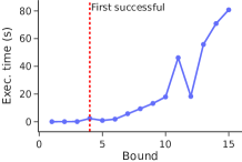
There is an obvious trade-off about the choice of a variability bound (Thm. 3.2): bigger means the search is more extensive, but it incurs greater computational cost.
This tendency is confirmed in our experiments; the result for the benchmark is in Fig. 7 for illustration. Here, synthesis was successful for for the first time.
We also observe in the figure that computational cost is low when trace synthesis is unsuccessful. This suggests the following strategy: we start with small and increment it if trace synthesis is unsuccessful. We might waste time by trying too small ’s; but the wasted time should be small.
| STLts | Breach | ForeSee | bluSTL | STLmc | ||
| 0.1 | (3) | 59.4 | 546.8 | t/o | ||
| 0.3 | (4) | 9.3 | 104.3 | 14.3 | t/o | |
| 0.1 | (3) | 81.3 | 197.4 | t/o | ||
| 32.5 | (17) | 16.5 | ||||
| 2.1 | (11) | 10.0 | ||||
| 0.4 | (3) | 8.9 | t/o | |||
| 0.2 | (2) | t/o | t/o | |||
| 0.4 | (2) | t/o | t/o | |||
| 9.9 | (4) | 31.2 | 435.8 | |||
| 2.4 | (4) | t/o | 58.9 | |||
| 0.6 | (3) | 33.6 | 187.2 | |||
| 1.5 | (3) | 38.8 | t/o | |||
Experimental Results, Overview. Our experimental results are in summarized in Table 2, where the best performers are highlighted by color.
We explain the missing entries. In , the tool is not applicable due to the nondeterminism of the benchmark. In , we did not conduct experiments since the performance comparison with STLts is already clear with simpler benchmarks. In , bluSTL does not support multiple control modes. is because bluSTL (at least its implementation available to us) does not support the until modality.
Overall, our STLts is clearly the best performer in all benchmarks but one. The other tools time out, or takes tens of seconds. For our motivation of illustrating STL specs by trace synthesis in close interaction with users, tens of seconds is prohibitively long. The results adequately demonstrate satisfactory performance of our algorithm, in trace synthesis for complex STL specs.
| Feature | STLts | Breach/ForeSee | bluSTL | STLmc |
| Trace synthesis for analyzing specs | Successful in all benchmarks with large STL formulas | Good for falsifying models but not good with large STL formulas | - Timeout in most of benchmarks | Timeout except for linear dynamics |
| Model checking | Complete up to and | - | Control synthesis with guarantee | Complete up to |
| Parameter mining | By MILP | - | By MILP | By binary search |
| Continuous STL semantics | Variable-interval encoding | - Discretized | - Discretized | Variable-interval encoding |
| Accommodated class of nonlinear dynamics | MILP-encodable, can be nondeterministic | Black-box, deterministic | MILP-encodable, can be nondeterministic | SMT-encodable, can be nondeterministic |
-
•
= full support; = partial support; = very limited support; - = not supported.
RQ2: Comparison with Other Approaches. A summary of comparison is in Table 3. The comparison with optimization-based falsification tools is as we expected—their struggle with complex specs motivated this work (Section 1). Boolean connectives in STL specs have been found problematic in falsification: this is called the scale problem [39, 40]. The results in Table 2 show that our benchmark specs are even beyond the capability of ForeSee, a tool that incorporates Monte Carlo tree search to specifically handle the scale problem. After all, one can say that falsification tools are aimed at complex models, while our STLts is aimed at complex specs.
STLmc has a similar (“dual”) scope and utilizes a similar technique (stable partitioning) to our STLts; the main difference is that STLmc is SMT-based while STLts is MILP-based. Therefore STLts accommodates a smaller class of models, but it can be faster on them exploiting numeric optimization. Table 2 suggests the advantage of STLts for common STL specs in manufacturing.
RQ3: Performance in Real-World Scenarios. For this RQ, we refer to STLts’s performance on the ISO benchmarks. Illustrating the specs by trace synthesis is a real-world problem about safety standards for automated driving (Section 1), and Table 2 shows that STLts has sufficient performance and scalability to handle complex specs there (see 24).
RQ4: Performance in Parameter Mining.
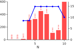
We conducted parameter mining experiments with the benchmark. Its specification has a subformula that requires that SV’s velocity is bigger than POV’s by at least a parameter . We used STLts to solve Thm. 3.3, that is, to find the maximum for which a satisfying trace exists.
Fig. 8 shows the results with varying variability bound . Parameter mining is generally more expensive than trace synthesis. This is because the former has a nontrivial objective function (namely in this example), while the latter does not (it is thus a constraint satisfaction problem). We observe the optimization with resulted in a timeout. The tendency, much like in trace synthesis, is that the result (max ) improves but execution time gets larger as becomes bigger (there are some exceptions such as though). Taking the same strategy as above (incrementing ), it takes roughly 10 minutes to obtain a largely converged value ( for the maximum ). Overall, we believe this is a realistic performance for practical usage.
References
- [1] ForeSee falsification solver (2021), https://github.com/choshina/ForeSee
- [2] Akazaki, T., Hasuo, I.: Time robustness in MTL and expressivity in hybrid system falsification. In: Kroening, D., Pasareanu, C.S. (eds.) Computer Aided Verification - 27th International Conference, CAV 2015, San Francisco, CA, USA, July 18-24, 2015, Proceedings, Part II. Lecture Notes in Computer Science, vol. 9207, pp. 356–374. Springer (2015). https://doi.org/10.1007/978-3-319-21668-3_21
- [3] Alur, R., Feder, T., Henzinger, T.A.: The Benefits of Relaxing Punctuality. Journal of the ACM 43(1), 116–146 (1996). https://doi.org/10.1145/227595.227602
- [4] Asarin, E., Donzé, A., Maler, O., Nickovic, D.: Parametric identification of temporal properties. In: Khurshid, S., Sen, K. (eds.) Runtime Verification - Second International Conference, RV 2011, San Francisco, CA, USA, September 27-30, 2011, Revised Selected Papers. Lecture Notes in Computer Science, vol. 7186, pp. 147–160. Springer (2011). https://doi.org/10.1007/978-3-642-29860-8_12
- [5] Asghari, M., Fathollahi-Fard, A.M., Mirzapour Al-e hashem, S.M.J., Dulebenets, M.A.: Transformation and linearization techniques in optimization: A state-of-the-art survey. Mathematics 10(2) (2022). https://doi.org/10.3390/math10020283
- [6] Atkinson, K.E.: An Introduction to Numerical Analysis. John Wiley & Sons, New York, second edn. (1989), http://www.worldcat.org/isbn/0471500232
- [7] Bae, K., Lee, J.: Bounded model checking of signal temporal logic properties using syntactic separation. Proceedings of the ACM on Programming Languages 3(POPL), 51:1–51:30 (Jan 2019). https://doi.org/10.1145/3290364
- [8] Bartocci, E., Deshmukh, J.V., Donzé, A., Fainekos, G., Maler, O., Nickovic, D., Sankaranarayanan, S.: Specification-based monitoring of cyber-physical systems: A survey on theory, tools and applications. In: Bartocci, E., Falcone, Y. (eds.) Lectures on Runtime Verification - Introductory and Advanced Topics, Lecture Notes in Computer Science, vol. 10457, pp. 135–175. Springer (2018). https://doi.org/10.1007/978-3-319-75632-5_5
- [9] Bartocci, E., Mateis, C., Nesterini, E., Nickovic, D.: Survey on mining signal temporal logic specifications. Inf. Comput. 289(Part), 104957 (2022). https://doi.org/10.1016/J.IC.2022.104957
- [10] Bu, L., Frehse, G., Kundu, A., Ray, R., Shi, Y., Zaffanella, E.: Arch-comp22 category report: Hybrid systems with piecewise constant dynamics and bounded model checking. In: Frehse, G., Althoff, M., Schoitsch, E., Guiochet, J. (eds.) Proceedings of 9th International Workshop on Applied Verification of Continuous and Hybrid Systems (ARCH22). EPiC Series in Computing, vol. 90, pp. 44–57. EasyChair (2022). https://doi.org/10.29007/lnzf
- [11] Donzé, A.: Breach, A toolbox for verification and parameter synthesis of hybrid systems. In: Touili, T., Cook, B., Jackson, P.B. (eds.) Computer Aided Verification, 22nd International Conference, CAV 2010, Edinburgh, UK, July 15-19, 2010. Proceedings. Lecture Notes in Computer Science, vol. 6174, pp. 167–170. Springer (2010). https://doi.org/10.1007/978-3-642-14295-6_17
- [12] Donzé, A., Ferrère, T., Maler, O.: Efficient robust monitoring for stl. In: Sharygina, N., Veith, H. (eds.) Computer Aided Verification. pp. 264–279. Springer Berlin Heidelberg, Berlin, Heidelberg (2013)
- [13] Donzé, A., Maler, O.: Robust satisfaction of temporal logic over real-valued signals. In: Chatterjee, K., Henzinger, T.A. (eds.) Formal Modeling and Analysis of Timed Systems - 8th International Conference, FORMATS 2010, Klosterneuburg, Austria, September 8-10, 2010. Proceedings, Lecture Notes in Computer Science, vol. 6246, pp. 92–106. Springer (2010). https://doi.org/10.1007/978-3-642-15297-9_9
- [14] Donzé, A., Raman, V.: BluSTL: Controller Synthesis from Signal Temporal Logic Specifications. In: ARCH14-15. 1st and 2nd International Workshop on Applied veRification for Continuous and Hybrid Systems. pp. 160–150. https://doi.org/10.29007/g39q
- [15] Duggirala, P.S., Mitra, S.: Abstraction Refinement for Stability. In: 2011 IEEE/ACM Second International Conference on Cyber-Physical Systems. pp. 22–31. IEEE (2011). https://doi.org/10.1109/ICCPS.2011.24
- [16] Ernst, G., Arcaini, P., Bennani, I., Chandratre, A., Donzé, A., Fainekos, G., Frehse, G., Gaaloul, K., Inoue, J., Khandait, T., Mathesen, L., Menghi, C., Pedrielli, G., Pouzet, M., Waga, M., Yaghoubi, S., Yamagata, Y., Zhang, Z.: ARCH-COMP 2021 category report: Falsification with validation of results. In: Frehse, G., Althoff, M. (eds.) 8th International Workshop on Applied Verification of Continuous and Hybrid Systems (ARCH21), Brussels, Belgium, July 9, 2021. EPiC Series in Computing, vol. 80, pp. 133–152. EasyChair (2021). https://doi.org/10.29007/XWL1
- [17] Fainekos, G.E., Pappas, G.J.: Robustness of temporal logic specifications for continuous-time signals. Theoretical Computer Science 410(42), 4262–4291 (Sep 2009). https://doi.org/10.1016/j.tcs.2009.06.021
- [18] Glover, F.: Improved linear integer programming formulations of nonlinear integer problems. Management Science 22, 455–460 (12 1975). https://doi.org/10.1287/mnsc.22.4.455
- [19] Gupte, A., Ahmed, S., Cheon, M.S., Dey, S.: Solving mixed integer bilinear problems using milp formulations. SIAM Journal on Optimization 23(2), 721–744 (2013). https://doi.org/10.1137/110836183
- [20] Gurobi Optimization, LLC: Gurobi Optimizer Reference Manual (2023), https://www.gurobi.com
- [21] Henzinger, T.A., Kopke, P.W.: Discrete-time control for rectangular hybrid automata. In: Degano, P., Gorrieri, R., Marchetti-Spaccamela, A. (eds.) Automata, Languages and Programming, 24th International Colloquium, ICALP’97, Bologna, Italy, 7-11 July 1997, Proceedings. Lecture Notes in Computer Science, vol. 1256, pp. 582–593. Springer (1997). https://doi.org/10.1007/3-540-63165-8_213
- [22] Henzinger, T.A., Kopke, P.W., Puri, A., Varaiya, P.: What’s decidable about hybrid automata? In: Leighton, F.T., Borodin, A. (eds.) Proceedings of the Twenty-Seventh Annual ACM Symposium on Theory of Computing, 29 May-1 June 1995, Las Vegas, Nevada, USA. pp. 373–382. ACM (1995). https://doi.org/10.1145/225058.225162
- [23] Road vehicles — Test scenarios for automated driving systems — Scenario based safety evaluation framework. Standard, International Organization for Standardization, Geneva, CH (Nov 2022)
- [24] Kurtz, V., Lin, H.: A more scalable mixed-integer encoding for metric temporal logic. IEEE Control. Syst. Lett. 6, 1718–1723 (2022). https://doi.org/10.1109/LCSYS.2021.3132839
- [25] Lee, J., Yu, G., Bae, K.: Efficient SMT-Based Model Checking for Signal Temporal Logic. In: 2021 36th IEEE/ACM International Conference on Automated Software Engineering (ASE). pp. 343–354 (Nov 2021). https://doi.org/10.1109/ASE51524.2021.9678719
- [26] Maler, O., Nickovic, D.: Monitoring temporal properties of continuous signals. In: Lakhnech, Y., Yovine, S. (eds.) Formal Techniques, Modelling and Analysis of Timed and Fault-Tolerant Systems, Joint International Conferences on Formal Modelling and Analysis of Timed Systems, FORMATS 2004 and Formal Techniques in Real-Time and Fault-Tolerant Systems, FTRTFT 2004, Grenoble, France, September 22-24, 2004, Proceedings. Lecture Notes in Computer Science, vol. 3253, pp. 152–166. Springer (2004). https://doi.org/10.1007/978-3-540-30206-3_12
- [27] Pedrielli, G., Khandait, T., Cao, Y., Thibeault, Q., Huang, H., Castillo-Effen, M., Fainekos, G.: Part-X: A family of stochastic algorithms for search-based test generation with probabilistic guarantees. IEEE Transactions on Automation Science and Engineering pp. 1–22 (2023). https://doi.org/10.1109/TASE.2023.3297984
- [28] Prabhakar, P., Lal, R., Kapinski, J.: Automatic Trace Generation for Signal Temporal Logic. In: 2018 IEEE Real-Time Systems Symposium (RTSS). pp. 208–217. IEEE, Nashville, TN (Dec 2018). https://doi.org/10.1109/RTSS.2018.00038
- [29] Rabinovich, A.M.: On the Decidability of Continuous Time Specification Formalisms. Journal of Logic and Computation 8(5), 669–678 (Oct 1998). https://doi.org/10.1093/logcom/8.5.669
- [30] Raman, V., Donzé, A., Maasoumy, M., Murray, R.M., Sangiovanni-Vincentelli, A.L., Seshia, S.A.: Model predictive control with signal temporal logic specifications. In: 53rd IEEE Conference on Decision and Control, CDC 2014, Los Angeles, CA, USA, December 15-17, 2014. pp. 81–87. IEEE (2014). https://doi.org/10.1109/CDC.2014.7039363
- [31] Raman, V., Donzé, A., Sadigh, D., Murray, R.M., Seshia, S.A.: Reactive synthesis from signal temporal logic specifications. In: Proceedings of the 18th International Conference on Hybrid Systems: Computation and Control. pp. 239–248. ACM, Seattle Washington (Apr 2015). https://doi.org/10.1145/2728606.2728628
- [32] Reimann, J., Mansion, N., Haydon, J., Bray, B., Chattopadhyay, A., Sato, S., Waga, M., Étienne André, Hasuo, I., Ueda, N., Yokoyama, Y.: Temporal logic formalisation of ISO 34502 critical scenarios: Modular construction with the RSS safety distance. In: Proc. the 39th ACM/SIGAPP Symposium on Applied Computing (SAC 2024) (2024), to appear. Preprint available as arXiv:2403.18764
- [33] Roehm, H., Heinz, T., Mayer, E.C.: Stlinspector: STL validation with guarantees. In: Majumdar, R., Kuncak, V. (eds.) Computer Aided Verification - 29th International Conference, CAV 2017, Heidelberg, Germany, July 24-28, 2017, Proceedings, Part I. Lecture Notes in Computer Science, vol. 10426, pp. 225–232. Springer (2017). https://doi.org/10.1007/978-3-319-63387-9_11, https://doi.org/10.1007/978-3-319-63387-9_11
- [34] Sato, S., An, J., Zhang, Z., Hasuo, I.: Optimization-based model checking and trace synthesis for complex stl specifications (extended version) (Jun 2024)
- [35] Souyris, J., Wiels, V., Delmas, D., Delseny, H.: Formal verification of avionics software products. In: Cavalcanti, A., Dams, D. (eds.) FM 2009: Formal Methods, Second World Congress, Eindhoven, The Netherlands, November 2-6, 2009. Proceedings. Lecture Notes in Computer Science, vol. 5850, pp. 532–546. Springer (2009). https://doi.org/10.1007/978-3-642-05089-3_34
- [36] Wolff, E.M., Topcu, U., Murray, R.M.: Optimization-based trajectory generation with linear temporal logic specifications. In: 2014 IEEE International Conference on Robotics and Automation (ICRA). pp. 5319–5325. IEEE, Hong Kong, China (May 2014). https://doi.org/10.1109/ICRA.2014.6907641
- [37] Yu, G., Lee, J., Bae, K.: Stlmc: Robust STL model checking of hybrid systems using SMT. In: Shoham, S., Vizel, Y. (eds.) Computer Aided Verification - 34th International Conference, CAV 2022, Haifa, Israel, August 7-10, 2022, Proceedings, Part I. Lecture Notes in Computer Science, vol. 13371, pp. 524–537. Springer (2022). https://doi.org/10.1007/978-3-031-13185-1_26
- [38] Zhang, Z., Arcaini, P.: Gaussian process-based confidence estimation for hybrid system falsification. In: Huisman, M., Pasareanu, C.S., Zhan, N. (eds.) Formal Methods - 24th International Symposium, FM 2021, Virtual Event, November 20-26, 2021, Proceedings. Lecture Notes in Computer Science, vol. 13047, pp. 330–348. Springer (2021). https://doi.org/10.1007/978-3-030-90870-6_18
- [39] Zhang, Z., Hasuo, I., Arcaini, P.: Multi-armed bandits for boolean connectives in hybrid system falsification. In: Dillig, I., Tasiran, S. (eds.) Computer Aided Verification - 31st International Conference, CAV 2019, New York City, NY, USA, July 15-18, 2019, Proceedings, Part I. Lecture Notes in Computer Science, vol. 11561, pp. 401–420. Springer (2019). https://doi.org/10.1007/978-3-030-25540-4_23
- [40] Zhang, Z., Lyu, D., Arcaini, P., Ma, L., Hasuo, I., Zhao, J.: Effective hybrid system falsification using monte carlo tree search guided by qb-robustness. In: Silva, A., Leino, K.R.M. (eds.) Computer Aided Verification - 33rd International Conference, CAV 2021, Virtual Event, July 20-23, 2021, Proceedings, Part I. Lecture Notes in Computer Science, vol. 12759, pp. 595–618. Springer (2021). https://doi.org/10.1007/978-3-030-81685-8_29
Appendix 0.A Further Details
Definition 0.A.1 (STL (Boolean) semantics)
Let be a signal and be an STL formula, both over . The satisfaction relation between them is defined as follows; the semantics of the other operators are defined similarly [17].
Definition 0.A.2 (STL robust semantics)
Let be a signal and be an STL formula, both over . STL robust semantics returns a quantity that indicates the satisfaction level of to , defined as follows.
The semantics of the other operators are defined similarly [17].
It is well-known that, by the quantitative robust semantics, one can infer the Boolean semantics: if is positive, it implies that , and if is negative, it implies that .
Definition 0.A.3 (PSTL)
Let and be vectors of syntactic parameters; those in are called magnitude parameters and those in are timing parameters.
The syntax of parametric STL (PSTL) is obtained by extending that of STL (Thm. 2.5) as follows: 1) atomic propositions can also be in the form , having a magnitude parameter on the right-hand side instead of ; and 2) allowing a timing parameter as a bound of the interval that indexes a temporal operator or (i.e. or can be , instead of a constant).
Let and ; these are the value domains of the parameters . Let and be vectors of real numbers from the domains. Given a PSTL formula , by replacing the occurrences of and with and , we obtain an STL formula. It is denoted by .
The following is an easy consequence of Thm. 2.8: is obtained as a common refinement of partitions for subformulas.
Proposition 0.A.4
If is finitely variable with respect to , then there exists a stable partitioning of any interval for and . ∎
Under a stable partitioning for and , one can discretize according to truth values indexed by subformulas of and intervals .
Definition 0.A.5 ([7, Definition 5])
Let be an STL formula, be a partitioning of and be an assignment of Boolean values. A signal matches the pair if 1) is a stable partitioning for and , and 2) for each and , we have if and only if for each .
By Thm. 0.A.4, for any signal that is finitely variable with respect to , there exists that matches it. We note that it is sufficient to decide the value of for atomic propositions in order to identify ; the values for the other subformulas are then determined by the STL semantics.
Appendix 0.B Shorthands for Propositional Connectives
We use the following shorthands in our constraints, where are Boolean variables. They are standard in the MILP community; see e.g. [36].
| (25) |
We can also nest the shorthand expressions by introducing auxiliary variables.
Note that one can represent arbitrary nested relation by introducing auxiliary variable. For example, is a shorthand notation for and with a new auxiliary variable .
Appendix 0.C Rectangular Hybrid Automata (RHAs)
RHAs [22] are restricted hybrid automata and are thus suited to analysis by LP. We briefly review its theory, restricting some definitions for our convenience. We refer to [22, 21] for further details.
Let be a set of (real-valued) variables. A rectangular predicate over is one of the form where are real numbers or . We restrict to closed intervals for simplicity.
A rectangular hybrid automaton (RHA) over a set of variables is a hybrid automaton (HA) where 1) the flow dynamics at each control mode is described by a rectangular predicate over ; 2) the invariant at each control mode is a rectangular predicate over ; and 3) each transition between control modes is labeled with where is a rectangular predicate over , is a rectangular predicate over ( is “ after transition”); and is a subset.
The transition labeled with is enabled only when is true, and when it is taken, only the values of can be altered. The alteration of the values of is fully nondeterministic—the new values can be any reals—although the new values must satisfy .
The rest of the operational semantics is standard for HAs; this allows us to identify an RHA with a system model in the sense of Thm. 2.3, restricting the domain of signals by some . RHAs have no input; thus the input variable set is . The nondeterminism of RHAs is reflected in in the type of .
An example of an RHA is in our navigation case study; see Fig. 6.
An encoding of RHAs to MILP is not hard. For compatibility with the encoding of STL in Section 4, our encoding of RHAs is in a variable-interval style, too, where the time domain is discretized into intervals . Here all ’s are continuous MILP variables. Due to the restriction to rectangular predicates—the slope of dynamics is bounded by constants, in particular—the operational semantics of RHAs can be exactly encoded to MILP.