A three-layer model for the dam-break flow of
particulate suspensions driven by sedimentation

Abstract.

We introduce a system of Saint-Venant-type equations to model laboratory experiments of dam-break particle-laden flows. We explore homogeneous and non-cohesive liquid-solid suspensions of monodispersed glass beads that propagate as single-phase flows, forming a progressively growing deposit of particles at the bottom of a smooth channel and creating a thin layer of pure liquid at the surface. The novelty of this model is twofold. First, we fully characterize the first-order behavior of these flows (mean velocity, runout distances and deposits geometry) through the sole sedimentation process of the grains, thus avoiding the use of any artificial friction to stop the flow. The model remains very simple and turns out to be effective despite the complex nature of interactions involved in these phenomena. Secondly, the sedimentation dynamics of the grains is observed to not being mainly affected by the flow, but remains comparable to that measured in static suspensions. The mathematical model is validated by comparing the experimental kinematics and deposit profiles with the simulations. The results highlight that this simplified model is sufficient to describe the general features of these flows as well as their deposit morphology, provided that the settling rate is adjusted starting from a critical value of the Reynolds number where the flow agitation begins to significantly delay the mean sedimentation velocity.

Keywords: Geophysics; Dam-break particle-laden flows; Sedimentation-dominated dynamics;
                   Multi-layer shallow water model; Hydrostatic upwind finite volume scheme.

AMS Subject Classification: 86-10; 35Q86; 76B99; 76M12.

1. Introduction

Lahars are geophysical mass flows, made with hot volcanic ash and tephra or fluvial sediments suspended into water, that travel down valleys at high velocity under the influence of gravity. During propagation, their general behavior undergoes important modifications in particle concentration [49], thus evolving from slightly concentrated flows (with a solid concentration lower than $20\ \textrm{vol}\%$), to hyperconcentrated flows (with a solid concentration ranged from $20\ \mathrm{vol}\%$ to $50\ \mathrm{vol}\%$) or debris flows (with a solid concentration that exceeds $50\ \mathrm{vol}\%$) [40]. Such large-scale natural phenomena are highly hazardous and commonly drive to important damages [21]. In the aim of providing reliable tools to help local authorities to establish proper risk assessments and take relevant preventing decisions, it appears fundamental to understand the physical processes that govern the flow dynamics and to develop predictive models of their runout time, distance, and deposit geometry. Dam-break experiments involving particulate suspensions consist in the sudden release of a fluidized granular column, of known concentration, down a horizontal plane and provide a simplified way to describe such complex geophysical events. The study of canonical configurations of small-scale collapses thus became largely explored in the last decades, leading to the development of predictive laws guided by two complementary approaches.

The first one is based on a dimensional analysis which allows to identify the main physical parameters governing the flow dynamics, as a mean of deducing empirical laws that involve nondimensional groups and are able to describe the flow propagation (runout time and length, flow velocity) and their deposits. In recent years, small-scale experiments of granular slumping performed under controlled conditions in both axisymmetric and rectangular configurations have highlighted the description of the flow dynamics and deposit geometry in terms of the free fall collapse, described by the gravity time and speed, as well as the initial geometry of the column, described by its aspect ratio [27, 32]. Similar investigations of slightly expanded ($2.5$-$4.5\%$) gas-particles systems have exhibited the water-like behavior of these mixtures dominated by an excess of fluid pressure, and have also shown the dependency on the initial geometry of the slightly fluidized column [47, 46]. Additional experiments on highly expanded (up to $50\%$), fully fluidized, dam-break suspension flows have been conducted, highlighting the effect of the solid concentration on their dynamics dominated by the sedimentation processes that control the emplacement of such experimental and natural flows [16, 20]. In particular, the sedimentation velocity of particles was observed to not being affected by the flow, thus remaining comparable to that inferred from static suspensions that results from simple vertical collapse tests [16, 18]. Afterwards, dam-break avalanches of wet granular materials, involving both unsaturated and saturated mixtures, were developed and underlined the dependency on the particle concentration, as well as on the Bond and Stokes numbers to describe the column collapse and the dynamics [2, 10].

The second approach exploits these dimensional analyses, primarily established for the development of experimental scaling laws, to define the proper physical assumptions underlying the derivation of relevant partial differential equations of mass and momentum conservation, which can be used to model and simulate the flows [28, 14, 22, 23, 33]. Since the dynamics of geophysical mixtures may involve several complex mechanics such as dilatancy effects, inter-particle and fluid-grain friction, sedimentation, resuspension, particle segregation, it is important to identify the main processes of interest, depending on the phenomenon and on the scientific issues under consideration. Many scientific efforts devoted to the mathematical description of such phenomena have been developed in recent years, based on the leading idea that the flow evolves as a thin homogeneous layer in which horizontal motions are much greater than the vertical ones. The resulting models are thus obtained by depth-integrating Navier–Stokes equations in a thin-layer approximation. In particular, we can distinguish between single-phase models [23, 11, 12, 34], quasi single-phase models [24, 44, 25] where two equations are required for the mass conservation of both the mixture and the solid phase, while the relative motion and interactions between the fluid and the solid components are neglected, and two-phase models [41, 39, 37, 42, 26, 7, 8, 30] where a system of four coupled equations for mass and momentum conservation of each phase are needed to describe the evolution of the multi-phase flow. A distinct mention should be made for the multi-component models [35] and [4], which are based on a very general framework that considers the full Navier–Stokes equations for both the fluid and the solid phases, avoiding any depth-averaged approximation.

In this work, we aim at developing a series of small-scale laboratory experiments to study the propagation of homogeneous and non-cohesive suspensions made with monodispersed glass beads and water, down a horizontal channel. The suspensions, whose solid volume fractions range from $0.41$ to $0.53$, are obtained by fluidizing a granular material in a reservoir. Previous experimental investigations highlighted that the flow dynamics is primarily controlled by sedimentation, initiated after the gravitational collapse down the rectangular flume, until all particles have deposited and the flow is at rest, which provides a natural criterion for the stopping phase [18]. The sedimentation velocity appears to not being affected by the propagation, in the sense that it remains mostly constant with time and space and is well approximated by the one measured from the static regime. Starting from this analysis, we aim at proposing relevant simplified mathematical equations to model the experiments. We propose a multi-layer approach for describing the evolution of a suspension that behaves as an idealized equivalent non-turbulent fluid and forms a deposit that thickens with time as well as an upper layer of water originating from the loss of mass due to sedimentation. In particular, the resulting system of shallow water equations is obtained by depth-integrating a coupled incompressible Euler–Navier–Stokes formulation, that carefully accounts for the three evolving physical interfaces between the different layers. As such a system may loose its hyperbolicity due to the presence of different densities between layers [13], leading to possible numerical instabilities, we shall follow the strategy proposed by Berton et al. [5] to design our numerical method, making use of a change of variables that allows to switch into an apparent-depths formulation, where the new system is decoupled and hyperbolic in each apparent layer. Standard finite volume techniques can then be applied to discretize the numerical fluxes and simulate the equations. To predict the particle sedimentation rate from the mixture during propagation, we used a general law valid for suspensions of various concentrations (from the dilute regime to the denser ones) and involving all types of materials and fluids [1], when the fluid inertia remains negligible (i.e. in the case of a Stokes flow regime). This law includes the theoretical formulation of a single particle falling into a homogeneous fluid of equivalent properties (in term of mixture density and viscosity). This approach is thus limited to homogeneous cases that can be described using a one-phase model and does not include particles segregation, turbulent stresses or pore pressure effects [42, 26, 30, 4], which require a more general two-phase flow model to be appropriately characterized. Despite its simplicity, the proposed model can satisfyingly reproduce the first-order features of our dam-break flow experiments, which can be viewed as small-scale hyper-concentrated flows or lahars. In this framework, the model provides an original point of view including a depositional description that controls the general behavior of such suspension flows during their final stage of transport, when dominated by sedimentation.

The work is structured as follows. We first present the experimental device and the laboratory experiments in Section 2. Based on these observations, we formulate the main physical assumptions in Section 3 and we introduce the mathematical model, as well as the numerical strategy for the simulations. Section 4 is devoted to the comparison between numerical results and experiments. We conclude with some final remarks in Section 5.

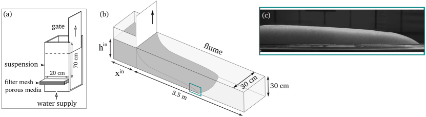
Figure 1.1. Experimental device: (a) Reservoir of the experimental device where suspensions are generated using a fluidization technique. (b) Dam-break flume where suspension flows are generated and explored through the transparent side walls. (c) Picture of a suspension flow made with glass beads and water.

2. Description of the experiments

2.1. Experimental procedure

The experiments consist in generating homogeneous particulate suspensions with fluidization techniques and in exploring their propagation when flowing down a horizontal, impermeable channel (see Figure 1.1). Solid particles of glass beads are first placed into a rectangular reservoir of $10\ \mathrm{cm}$-long, $30\ \mathrm{cm}$-wide and $70\ \mathrm{cm}$-high, where they form a granular column of solid volume fraction $\phi_{pack}$. A fluid (water, here) is then injected uniformly at a velocity $U_{f}$, at the base of the granular pile, passing through a porous medium. Above a threshold fluid velocity $U_{mf}$, particles become fully fluidized, so that the pressure gradient across the bed (fixed by the weight of the particles) becomes independent of $U_{f}$. In this state, the mixture forms a homogeneous, stable suspension of solid volume fraction $\phi_{s}$, whose expansion rate $\phi_{pack}/\phi_{s}$ is proportional to $U_{f}$ [17, 18]. Once obtained, the suspension of controlled density $\rho_{m}=\phi_{s}\rho_{s}+(1-\phi_{s})\rho_{f}$ is released down the flume of $3.5\ \mathrm{m}$-long and $30\ \mathrm{cm}$-wide, made with transparent side walls, as in the manner of a dam-break. This forms a fast-moving, but short-lived, free-surface flow that sediments progressively during its travel and until motion ceases. During its propagation, the flow has been recorded using a semi-fast camera to capture the frontal kinematics and runouts. At the end of the experiments, the deposit geometry has been carefully measured. The series of experiments presented here involves quasi-spherical, smooth glass beads (whose features are presented in Table 2.1) mixed with water taken at room temperature (20${}^{o}C$), of density $\rho_{f}=1000\ \mathrm{kg\cdot m^{-3}}$ and dynamic viscosity $\mu_{f}=10^{-3}\ \mathrm{Pa\cdot s}$.

$Material$	$d\leavevmode\nobreak\ (\mu\mathrm{m})$	$\rho_{s}\leavevmode\nobreak\ (\mathrm{kg\cdot m^{-3}})$	$\phi_{pack}$	$h_{s}\leavevmode\nobreak\ (\mathrm{cm})$	$h_{m}\leavevmode\nobreak\ (\mathrm{cm})$	$\phi_{s}/\phi_{pack}$
$GB$	$337$	$2496$	$0.58$	$19$ - $27$	$27$	$0.7$ - $1$

Table 2.1. Main experimental parameters: Physical properties of glass beads and suspensions involved in the dam-break flow experiments.

2.2. General behavior of the flows

When released, the particulate suspension travels down the flume at a mean velocity of up to $1.5\ \mathrm{m\cdot s^{-1}}$ and with a frontal speed of up to $2\ \mathrm{m\cdot s^{-1}}$. During propagation, the homogeneous mixture progressively sediments and develops an internal flow structure that can be separated into three main vertical layers: a static basal deposit that thickens progressively during the flow; a flowing suspension that thins progressively by expelling water upwards and particles downwards; an upper layer of water formed from particles deposition. As commonly observed in classical dam-break flows, the propagation of the flow front takes place in three phases: (1) a brief gravitational collapse where no sedimentation occurs; (2) a dominant phase of constant velocity where both solid deposition and fluid expel develop; (3) a short decelerating phase (see Figure 2.2). The dam-break flow of such complex suspensions exposes a simple and systematic behavior whose dynamics is mainly controlled by the sedimentation processes, described by the sedimentation velocity $U_{sed}^{\mathsf{static}}$ that strongly depends on the mixture concentration $\phi_{s}/\phi_{pack}$ for a given material. The series of experiments presented here allows us to vary $\phi_{s}/\phi_{pack}$ from $0.7$ to $1$ (with a solid volume fraction $\phi_{s}$ that ranges from $0.4$ to $0.58$) and to explore the spreading of homogeneous and stable suspensions.

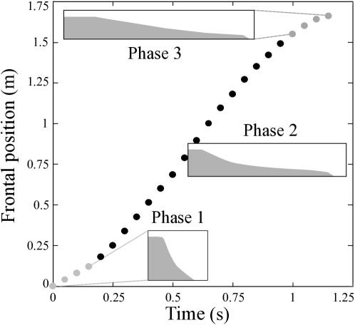
Figure 2.2. Kinematic profile of the flow front: Three main phases of transport observed in experimental dam-break flows.

2.3. The sedimentation law

The sedimentation processes that govern the runout of the dam-break suspension flows have been studied in details inside the reservoir, for cases where the particle inertia is negligible compared to the viscous stresses, i.e. in the Stokes flow regime, with the aim of determining a unified sedimentation law for a wide range of particle concentrations. Different series of experiments were carried out, involving homogeneous mixtures of synthetical materials (glass and PMMA beads, FCC catalysts) or natural ones (sands, volcanic ash) characterized by a mean grain diameter that ranged from $65$ to $350\ \mu\mathrm{m}$ and a solid density that ranged from $1200$ to $2650\ \mathrm{kg\cdot m^{-3}}$ suspended in different types of fluids (air or water) of contrasted density (from $0.8$ to $1000\ \mathrm{kg\cdot m^{-3}}$) and viscosity (from $10^{-3}$ to $10^{-5}\ \mathrm{Pa\cdot s}$).

The sedimentation velocity $U_{sed}^{\mathsf{static}}$ was measured after cutting the fluid supply at a given mixture concentration $\phi_{s}/\phi_{pack}$ [17]. Results analyses revealed that $U_{sed}^{\mathsf{static}}$ is controlled by three independent parameters [1], being the solid volume fraction $\phi_{s}$, the microstructure of interstices $\phi_{s}/\phi_{pack}$ and the Stokes number based on the Stokes velocity $St_{0}=\frac{g(\rho_{s}-\rho_{f})(\rho_{s}+\frac{1}{2}\rho_{f})d^{3}}{18\leavevmode\nobreak\ \mu_{f}^{2}}$, and that it can be approximated by the following general law

$$U_{sed}^{\mathsf{static}}=\frac{g(\rho_{s}-\rho_{f})d^{2}}{18\mu_{f}}(1-\phi_{s})\mathcal{F}_{1}\left(\frac{\phi_{s}}{\phi_{pack}}\right)\mathcal{F}_{2}\left(St_{0}\right),$$ (2.1)

$$\mathcal{F}_{1}(x)=\frac{e^{-3}+0.08}{e^{-3(1-x)}+0.08(1-x)^{-2/3}},$$ (2.2)

$$\mathcal{F}_{2}(x)=\frac{\frac{1}{45}x+1}{\frac{3}{45}x+1},$$ (2.3)

where the two first terms $\frac{g(\rho_{s}-\rho_{f})d^{2}}{18\mu_{f}}(1-\phi_{s})$ of equation (2.1) describe the velocity of a single particle of density $\rho_{s}$, with no inertia ($St_{0}=0$), immersed in a pure fluid ($\phi_{s}=0$) of high viscosity ($Re=0$) and characterized by a density $\rho_{m}=\phi_{s}\rho_{s}+(1-\phi_{s})\rho_{f}$, equivalent to that of the suspension. Note that $(\rho_{s}-\rho_{f})(1-\phi_{s})=\rho_{s}-\rho_{m}$, amounts to include the effect of the mixture density in the Stokes velocity, through the buoyancy acting on each particle. The third and fourth terms $\mathcal{F}_{1}\left(\frac{\phi_{s}}{\phi_{pack}}\right)$ and $\mathcal{F}_{2}\left(St_{0}\right)$ describe the effect of the mixture viscosity $\mu_{m}$ of the equivalent fluid on the particle sedimentation $U_{sed}^{\mathsf{static}}$, by taking into account the mixture concentration described by $\phi_{s}/\phi_{pack}$ and the particle inertia described by $St_{0}$.

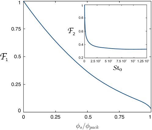
Figure 2.3. Shape of $\bm{\mathcal{F}_{1}}$ and $\bm{\mathcal{F}_{2}}$: Decreasing functions that describe the effect of the particle concentration in the mixture and that of the particle inertia on the sedimentation velocity, respectively expressed by (2.2) and (2.3).

These effects are described by independent decreasing functions, plotted in Figure 2.3. The sedimentation velocity of homogeneous suspensions turns out to be much smaller than that measured in a pure fluid at rest or in a cloud of particles that behaves as a cluster [36], due to the streamlines that pass all around the particles, thus increasing the drag force exerted on them. This unified law, valid for different types of non-cohesive particles and fluids, can be used to describe the sedimentation process in rapid dam-break flows of particulate suspensions in which deposition develops in the Stokes regime, despite the high Reynolds number of the flow based on the mean flow velocity [18, 19].

3. A three-layer depth-averaged model

In this part, we introduce the three-layer depth-averaged model developed to describe laboratory dam-break flows. We first present the main physical assumptions stemming from observations of experiments, then construct the mathematical description and discuss the numerical method used to simulate the physical model, while validating this in the following section through a direct comparison with the measurements.

3.1. Physical assumptions

Based on direct observations made on the general flow behavior, three main physical assumptions can be formulated in order to introduce the mathematical model.

• Structure of the dynamics. The dynamics of the flow is characterized by three phases of transport: an initial slumping phase with no sedimentation, during which the column collapses under the influence of gravity; a dominant propagation phase where the suspension travels down the flume at constant speed, while progressively depositing particles and expelling water; a final stopping phase where the flow decelerates until motion ceases, when all the particles have settled at the bottom of the flume.

• Structure of the flow. We assume that the particulate suspension is incompressible and develops three distinct homogeneous layers during its propagation: at the bottom, a non-moving deposit of volume fraction $\phi_{pack}$ and density $\rho_{d}=\rho_{s}\phi_{pack}+\rho_{f}(1-\phi_{pack})$ that grows over time due to the particles sedimentation from the above layer; a suspension of volume fraction $\phi_{s}$ and density $\rho_{m}=\rho_{s}\phi_{s}+\rho_{f}(1-\phi_{s})$ that travels above the deposit, undergoing a basal friction proportional to $U_{sed}^{\mathsf{static}}$, and which progressively loses particles downwards and water upwards; an upper free-surface pure fluid layer of density $\rho_{f}$ developed from the water expelled by the suspension, that travels without encountering any friction. The process of phase separation into these three layers is represented in Figure 3.4.

• Sedimentation process. The settling of particles develops at a rate $R_{sed}$ uniform in time and space over the moving domain of the flow, which is given explicitly by the formula

  $$R_{sed}=\frac{\rho_{s}}{\rho_{s}-\rho_{f}}\frac{U_{sed}^{\mathsf{dynamic}}}{\frac{\phi_{pack}}{\phi_{s}}-1},$$ (3.4)

  where the dynamical settling speed of the grains $U_{sed}^{\mathsf{dynamic}}=C(Re)U_{sed}^{\mathsf{static}}$ is proportional to the reference sedimentation velocity determined in the quasi-static configuration. In particular, the proportionality coefficient $C(Re)>0$ depends on the flow’s Reynolds number $Re=\frac{\rho_{f}dU_{mean}}{\mu_{f}}$, which is based on the mean flow velocity $U_{mean}$ measured in the experiments, the fluid properties described by $\rho_{f}$ and $\mu_{f}$, and the particle size given by the grain diameter $d$.

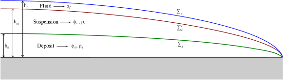
Figure 3.4. Internal flow structures: Vertical stratification developed during propagation, due to the separation of the two phases and leading to the formation of three different layers (basal deposit, flowing suspension and expelled fluid).

3.2. Governing equations

We develop our mathematical model under the above assumptions. Given the dimensions of the flume, we consider depth-averaged equations with negligible boundary effects.

Modeling the slumping phase. When the particulate suspension is released down the flume, the collapse of the initial column is essentially governed by gravitational forces. From experimental analyses, we observed that the main features of this phase corresponds to that observed in classical gravitational collapses. In particular, as the initial aspect ratio of the column $\frac{h^{\mathrm{in}}}{x^{\mathrm{in}}}>1$ (where $h^{\mathrm{in}}$ and $x^{\mathrm{in}}$ represents the column height and length, respectively) plays a major role in the slumping dynamics, simple shallow water models fail to capture the correct acceleration of the front since the thin-layer assumption is not satisfied in this regime. In order to avoid resorting to a full Navier–Stokes formulation which is computationally more expensive, we introduce a suitable model to describe the (short) initial phase in cases where the aspect ratio is high, and then reduce the study to standard shallow water equations as soon as the flow reaches a thin layer regime. The strategy that we follow to solve this problem has been proposed in the work by Larrieu et al. [29], where the collapse of a granular column is considered as free-falling into a moving flow of small aspect ratio $\varepsilon\ll 1$, whose dynamics can be described using shallow water equations.

In practice, we suppose from H1 that the suspension properties are constant in time and space, meaning that the suspension remains homogeneous with a constant volume fraction $\phi_{s}$ and density $\rho_{m}$, and that no sedimentation occurs during the initial collapse. The evolution of the suspension is thus characterized by its height $h=h(t,x)$ and by its mean lateral velocity $\bar{u}=\bar{u}(t,x)$, which both depend on time $t\in(0,t_{ff}]$ and space $x\in\mathbb{R}_{+}$. Then, the collapsing column of initial height $h^{\mathrm{in}}$ can be modeled as the evolution of a thin-layer flow of apparent initial height $h_{app}=\varepsilon x^{\mathrm{in}}$, with $\varepsilon\ll 1$, through the frictionless shallow water equations

$$\begin{split}&\partial_{t}h+\partial_{x}(h\bar{u})=S_{slump},\\[5.69054pt] &\partial_{t}(h\bar{u})+\partial_{x}(h\bar{u}^{2})=S_{slump}\bar{u}-gh\partial_{x}h,\end{split}$$ (3.5)

where the source term $S_{slump}=S_{slump}(t,x)$ is defined as :

$$S_{slump}(t,x)=gt\chi(0<t\leq t_{ff})\chi(0\leq x\leq x^{\mathrm{in}}),$$ (3.6)

and translates the raining of particles into the moving flow, over the spatial domain $x\in[0,x^{\mathrm{in}}]$ and during a time interval $t\in(0,t_{ff}]$. Here, $\chi(I)$ denotes the indicator function of the interval $I\subset\mathbb{R}_{+}$, $x^{\mathrm{in}}$ is the length of the reservoir and $t_{ff}$ is the typical time taken by a particle of density $\rho_{m}$ to fall from the height $h^{\mathrm{in}}$ to the apparent height $h_{app}$, defined as

$$t_{ff}=\left(\frac{2(h^{\mathrm{in}}-h_{app})}{g}\right)^{1/2}.$$ (3.7)

Modeling the layers interfaces. Following hypothesis H2, as soon as the gravitational slumping is over after the critical time $t_{ff}$, the suspension propagates at constant speed down the flume and forms three distinct homogeneous layers. For any $t>t_{ff}$ and $x\in\mathbb{R}_{+}$, we denote with $h_{d}=h_{d}(t,x)$, $h_{m}=h_{m}(t,x)$ and $h_{f}=h_{f}(t,x)$ the heights of the deposit of solid volume fraction $\phi_{pack}$ and density $\rho_{d}$, the height of the homogeneous mixture of solid volume fraction $\phi_{s}$ and density $\rho_{m}$, and that of the pure fluid of density $\rho_{f}$, respectively. Moreover, owing to the assumption that the incompressible flow can be described by the evolution of its longitudinal profile and that particles cease to move after settling, we also need to introduce the velocity fields (horizontal and vertical velocities) of the suspension $(u,w)$ and of the fluid $(U,W)$. Here, $u=u(t,x,z)$ and $w=w(t,x,z)$ are defined for $t>t_{ff}$, $x\in\mathbb{R}_{+}$ and $h_{d}\leq z\leq h_{m}$, while $U=U(t,x,z)$ and $W=W(t,x,z)$ are defined for $t>t_{ff}$, $x\in\mathbb{R}_{+}$ and $h_{m}\leq z\leq h_{f}$.

Then, the moving interfaces that characterize the evolution of each layer surface after the critical time $t_{ff}$ are modeled by the following equations

$$\partial_{t}h_{f}+U|_{z=h_{f}}\partial_{x}h_{f}-W|_{z=h_{f}}=0,$$ (3.8)

$$\partial_{t}h_{m}+u|_{z=h_{m}}\partial_{x}h_{m}-w|_{z=h_{m}}=-\left(\frac{\phi_{pack}}{\phi_{s}}-1\right)S_{sed},$$ (3.9)

$$\partial_{t}h_{d}=S_{sed},$$ (3.10)

where the source term $S_{sed}=S_{sed}(t)$ is defined as

$$S_{sed}(t)=R_{sed}\chi(t>t_{ff}),$$

and accounts for the sedimentation of particles from the suspension over the moving domain of the flow. We stress once more that no velocity field appears in equation (3.10), since the particles stop moving once they have settled to form the deposit. In particular, their sedimentation rate $R_{sed}$ is prescribed by hypothesis H3, using the explicit form (3.4), and is initiated after the initial slumping time $t_{ff}$. Notice that the resulting loss of particles in the overlying suspension is taken into account by the right-hand side of (3.9), which simply stems from a mass-conservation principle. At last, the absence of a source term in the fluid-layer equation (3.8) comes from the free-surface flow modeling.

The full depth-averaged model. We now have all the tools to introduce our model. Under the effect of gravity, the suspension and fluid layers can be described by classical incompressible Navier–Stokes and Euler equations, governing the evolution of their velocity fields $(u,w)$ and $(U,W)$ respectively. This modeling choice is a consequence of hypothesis H2, where the fluid flows is assumed frictionless over the suspension, while the latter undergoes a basal friction when flowing over the deposit. The last property is recovered by imposing a Navier-like condition at the interface with the deposit [15], namely

$$\left(\kappa u-\mu_{m}\partial_{z}u\right)|_{z=h_{d}}=0,\quad t>t_{ff},\ x\in\mathbb{R}_{+},$$

where $\kappa$ and $\mu_{m}$ denote respectively the basal friction coefficient and the dynamic viscosity of the suspension. The additional boundary conditions used to close the resulting Euler–Navier–Stokes system are detailed in Appendix B.

Let us now consider a thin-layer approximation of aspect ratio $\varepsilon=\frac{h_{0}}{L_{0}}$ where $h_{0}$ and $L_{0}$ denote characteristic dimensions for the height and length of the flow. By properly rescaling the Euler–Navier–Stokes system, we look at a particular regime of low friction where $\kappa$ is taken to be $\mathcal{O}(\varepsilon)$. Then, keeping in mind the equations for the three interfaces (3.8)–(3.10), we apply similar arguments to those presented in the work of Gerbeau and Perthame [15] to derive (see Appendix B), for $\varepsilon\ll 1$, the shallow water system

$$\partial_{t}H+\partial_{x}(H\bar{U})=\left(\frac{\phi_{pack}}{\phi_{s}}-1\right)S_{sed},$$ (3.11)

$$\partial_{t}(H\bar{U})+\partial_{x}(H\bar{U}^{2})=\left(\frac{\phi_{pack}}{\phi_{s}}-1\right)S_{sed}\bar{U}-gH\partial_{x}(H+h+h_{d}),$$ (3.12)

$$\partial_{t}h+\partial_{x}(h\bar{u})=S_{slump}-\frac{\phi_{pack}}{\phi_{s}}S_{sed},$$ (3.13)

$$\partial_{t}(h\bar{u})+\partial_{x}(h\bar{u}^{2})=\left(S_{slump}-\frac{\phi_{pack}}{\phi_{s}}S_{sed}\right)\bar{u}-\kappa\bar{u}\chi(t>t_{ff})-gh\partial_{x}\left(\frac{\rho_{f}}{\rho_{m}}H+h+h_{d}\right),$$ (3.14)

where (3.11)–(3.12) and (3.13)–(3.14) expresses the mass and momentum conservation for the fluid and suspension layers respectively, prescribing the evolution of their flows over $t>0$ and $x\in\mathbb{R}_{+}$ through the vertically-averaged quantities of heights $H=H(t,x)$, $h=h(t,x)$, and mean velocities $\bar{U}=\bar{U}(t,x)$, $\bar{u}=\bar{u}(t,x)$. These are defined as $H:=h_{f}-h_{m}$, $h:=h_{m}-h_{d}$, and $\bar{U}:=\frac{1}{H}\int_{h_{m}}^{h_{f}}U(t,x,z)\mathrm{d}z$, $\bar{u}:=\frac{1}{h}\int_{h_{d}}^{h_{m}}u(t,x,z)\mathrm{d}z$.

We first highlight that equations (3.10)–(3.14) are compatible with the modeling of the gravitational slumping, since they reduce to equation (3.5) in the time interval $[0,t_{ff}]$. Indeed, the particles settling does not occur during the initial phase since all source terms depending on $R_{sed}$ are activated after $t_{ff}$, implying that nor deposit or fluid layers are generated during the column collapse. The sedimentation process is also mass-preserving, a property that stems directly from the definition of the layer interfaces (3.8)–(3.10). This is not true for the conservation of momentum, when an additional basal friction $\kappa$ is imposed at the interface with the deposit. In what follows, $\kappa$ is chosen proportional to the sedimentation rate, and in particular $\kappa=R_{sed}/2$. The physical interpretation of this choice lies in the loss of mass by sedimentation which leads to a decrease in velocity, coherently with observations and measurements made from erosion processes in natural flows [43]. Moreover, the flow stratification into distinct sublayers is not considered here for numerical purposes, as in classical multi-layer shallow water systems [3], but is based on experimental observations and is characterized by well-defined physical interfaces. This feature is reflected by the term $g\frac{\rho_{f}}{\rho_{m}}h\partial_{x}H$ in equation (3.14), coming from the pressure balance at the interface between the suspension of density $\rho_{m}$ and the overlying fluid-layer of density $\rho_{f}$. In particular, the model (3.11)–(3.14) is only conditionally hyperbolic, depending on the value of the ratio $\frac{\rho_{f}}{\rho_{m}}$, a typical problematic of two-layer shallow water systems that shall be further discussed in the following section.

3.3. Numerical strategy

The numerical treatment of two-layer shallow water systems is rather delicate. The presence of the non-conservative products $H\partial_{x}h$ and $h\partial_{x}H$ leads to the lack of a conservation form for (3.11)–(3.14) and to the impossibility of properly characterizing discontinuous solutions through the Rankine–Hugoniot relations. Additionally, the system is hyperbolic only in a regime where the density ratio $\frac{\rho_{f}}{\rho_{m}}\ll 1$ is very small [13]. As these issues require the design of sophisticated numerical schemes to deal with the full two-layer model [38], it would be better to approximate equations (3.11)–(3.12) and (3.13)–(3.14) for each layer separately, since they are unconditionally hyperbolic. This would allow in particular to take advantage of standard finite volume solvers. However, using a scheme for each layer independently may lead to instabilities because of the non-conservative products, and thus need the careful development of a suitable decoupling strategy [9, 5]. Here, we shall make use of a splitting strategy based on a hydrostatic upwind scheme recently proposed by Berthon et al. [5], and then combine it with the HLL solver to deal with the resulting numerical fluxes.

The leading idea is to reformulate equations (3.11)–(3.14) in terms of the characteristic heights $h_{1}=H+h+h_{d}$ and $h_{2}=\frac{\rho_{f}}{\rho_{m}}H+h+h_{d}$, naturally arising from a computation of the steady states, and of the corresponding relative heights $X_{1}=\frac{H}{h_{1}}$ and $X_{2}=\frac{h}{h_{2}}$. After some simple algebraic manipulations, we obtain the transformed system

$$\partial_{t}H+\partial_{x}(X_{1}h_{1}\bar{U})=\left(\frac{\phi_{pack}}{\phi_{s}}-1\right)S_{sed},$$

$$\partial_{t}(H\bar{U})+\partial_{x}\left(X_{1}\left(h_{1}\bar{U}^{2}+\frac{g}{2}h_{1}^{2}\right)\right)=\left(\frac{\phi_{pack}}{\phi_{s}}-1\right)S_{sed}\bar{U}$$

$$\hskip 142.26378pt+\frac{g}{2}\partial_{x}\big{(}H(h_{1}-H)\big{)}-gH\partial_{x}(h_{1}-H),$$

$$\partial_{t}h+\partial_{x}(X_{2}h_{2}\bar{u})=S_{slump}-\frac{\phi_{pack}}{\phi_{s}}S_{sed},$$

$$\partial_{t}(h\bar{u})+\partial_{x}\left(X_{2}\left(h_{2}\bar{u}^{2}+\frac{g}{2}h_{2}^{2}\right)\right)=\left(S_{slump}-\frac{\phi_{pack}}{\phi_{s}}S_{sed}\right)\bar{u}$$

$$\hskip 142.26378pt-\kappa\bar{u}\chi(t>t_{ff})+\frac{g}{2}\partial_{x}(h(h_{2}-h))-gh\partial_{x}(h_{2}-h),$$

where the coupling between layers is now taken into account solely through the variables $h_{1}$ and $h_{2}$. In particular, we can rewrite equations (3.10)–(3.14) under the more convenient form

$$\begin{split}&\partial_{t}w_{1}+\partial_{x}\big{(}X_{1}f(W_{1})\big{)}=P(H,h_{1})+S_{1}(\bar{U}),\\[5.69054pt] &\partial_{t}w_{2}+\partial_{x}\big{(}X_{2}f(W_{2})\big{)}=P(h,h_{2})+S_{2}(\bar{u}),\\[5.69054pt] &\partial_{t}h_{d}=S_{sed},\end{split}$$ (3.15)

by using the notations $w_{1}=(H,H\bar{U})^{\intercal}$ and $w_{2}=(h,h\bar{u})^{\intercal}$ for the original shallow water variables $W_{1}=(h_{1},h_{1}\bar{U})^{\intercal}$ and $W_{2}=(h_{2},h_{2}\bar{u})^{\intercal}$ for the new characteristic variables $f(W_{1})=\left(h_{1}\bar{U},h_{1}\bar{U}^{2}+\frac{g}{2}h_{1}^{2}\right)^{\intercal}$ and $f(W_{2})=\left(h_{2}\bar{u},h_{2}\bar{u}^{2}+\frac{g}{2}h_{2}^{2}\right)^{\intercal}$ for the fluxes, $P(H,h_{1})=\left(0,\frac{g}{2}\partial_{x}\big{(}H(h_{1}-H)\big{)}-gH\partial_{x}(h_{1}-H)\right)^{\intercal}$ and $P(h,h_{2})=\left(0,\frac{g}{2}\partial_{x}\big{(}h(h_{2}-h)\big{)}-gh\partial_{x}(h_{2}-h)\right)^{\intercal}$ for the pressure terms (notice that the structure of $f$ and $P$ is the same for the two layers, hence the notation with no dependence on the indices) and finally

$$\begin{split}&S_{1}(\bar{U})=\left(\begin{array}[]{c}\left(\frac{\phi_{pack}}{\phi_{s}}-1\right)S_{sed}\\[8.53581pt] \left(\frac{\phi_{pack}}{\phi_{s}}-1\right)S_{sed}\bar{U}\end{array}\right),\\[11.38109pt] &S_{2}(\bar{u})=\left(\begin{array}[]{c}S_{slump}-\frac{\phi_{pack}}{\phi_{s}}S_{sed}\\[8.53581pt] \left(S_{slump}-\frac{\phi_{pack}}{\phi_{s}}S_{sed}\right)\bar{u}-\kappa\bar{u}\chi(t>t_{ff})\end{array}\right),\end{split}$$

for the source terms involving the slumping process, the sedimentation of particles from the suspension and the friction.

The aim is to design a suitable finite volume scheme to approximate equation (3.15). For this, we introduce a time step $\Delta t>0$ and a space step $\Delta x>0$, and define corresponding uniform meshes $(t^{n})_{n\in\mathbb{N}}$ and $(x_{i+\frac{1}{2}})_{i\in\mathbb{N}}$ of $\mathbb{R}_{+}$, such that $t^{n}=n\Delta t$ and $x_{i+\frac{1}{2}}=\left(i+\frac{1}{2}\right)\Delta x$. Then, at each time $t^{n}$ and on each spatial cell $(x_{i-\frac{1}{2}},x_{i+\frac{1}{2}})$, we consider constant approximations of the original variables $w_{1,i}^{n}=(H_{i}^{n},H_{i}^{n}\bar{U}_{i}^{n})^{\intercal}$ and $w_{2,i}^{n}=(h_{i}^{n},h_{i}^{n}\bar{u}_{i}^{n})^{\intercal}$ and of the new ones, as

$$\begin{split}&h_{1,i}^{n}=H_{i}^{n}+h_{i}^{n}+h_{d,i}^{n}\quad\textrm{with}\quad X_{1,i}^{n}=\frac{H_{i}^{n}}{h_{1,i}^{n}},\\[5.69054pt] &h_{2,i}^{n}=\frac{\rho_{f}}{\rho_{s}}H_{i}^{n}+h_{i}^{n}+h_{d,i}^{n}\quad\textrm{with}\quad X_{2,i}^{n}=\frac{h_{i}^{n}}{h_{2,i}^{n}}.\end{split}$$

Moreover, we also introduce suitable discretizations for the following terms

$$\begin{split}&S_{slump,i}^{n}=gt^{n}\chi({0\leq x_{i}\leq x_{0}})\chi({0<t^{n}\leq t_{ff}}),\\[5.69054pt] &S_{sed}^{n}=R_{sed}\chi{t^{n}>t_{ff}},\end{split}$$

which are activated respectively during the initial slumping phase and during the following sedimentation-driven phase.

From here, the updated states $w_{1,i}^{n+1}$ and $w_{2,i}^{n+1}$ are determined through a two-step scheme in time. We first take into account the fluxes $f$ and the pressure terms $P$ to compute intermediate values $w_{1,i}^{*}$ and $w_{2,i}^{*}$ from the initial conditions $(w_{j,i}^{n})_{j=1,2}$ [5], namely

$$\begin{split}&w_{j,i}^{*}=w_{j,i}^{n}-\frac{\Delta t}{\Delta x}\Big{(}X_{j,i+\frac{1}{2}}^{n}f_{\Delta x}(W_{j,i}^{n},W_{j,i+1}^{n})-X_{j,i-\frac{1}{2}}^{n}f_{\Delta x}(W_{j,i-1}^{n},W_{j,i}^{n})\Big{)}\\[5.69054pt] &\hskip 170.71652pt+\frac{g}{2}\frac{\Delta t}{\Delta x}\left(\begin{array}[]{c}0\\[5.69054pt] h_{j,i-\frac{1}{2}}^{n}h_{j,i+\frac{1}{2}}^{n}(X_{j,i+\frac{1}{2}}^{n}-X_{j,i-\frac{1}{2}}^{n})\end{array}\right),\end{split}$$ (3.16)

for $j=1,2$, where the classical shallow water numerical fluxes $f_{\Delta x}=(f_{\Delta_{x}}^{h},f_{\Delta x}^{hu})^{\intercal}$ are approximated using the HLL solver [6], while the values $(h_{j,i+\frac{1}{2}}^{n})_{i\in\mathbb{N}}$ and $(X_{j,i+\frac{1}{2}}^{n})_{i\in\mathbb{N}}$, $j=1,2$, at the interfaces of the spatial grid are defined through an upwind method, having the form

$$\begin{split}&h_{j,i+\frac{1}{2}}^{n}=\left\{\begin{array}[]{ll}W_{j,i}^{n}&\quad\textrm{if}\ f_{\Delta x}^{h}(W_{j,i}^{n},W_{j,i+1}^{n})>0,\\[5.69054pt] W_{j,i+1}^{n}&\quad\textrm{elsewhere},\end{array}\right.\qquad j=1,2,\\[11.38109pt] &X_{1,i+\frac{1}{2}}^{n}=\left\{\begin{array}[]{ll}\frac{H_{i}^{n}}{h_{1,i}^{n}}&\quad\textrm{if}\ f_{\Delta x}^{h}(W_{1,i}^{n},W_{1,i+1}^{n})>0,\\[5.69054pt] \frac{H_{i+1}^{n}}{h_{1,i+1}^{n}}&\quad\textrm{elsewhere},\end{array}\right.\\[11.38109pt] &X_{2,i+\frac{1}{2}}^{n}=\left\{\begin{array}[]{ll}\frac{h_{i}^{n}}{h_{2,i}^{n}}&\quad\textrm{if}\ f_{\Delta x}^{h}(W_{2,i}^{n},W_{2,i+1}^{n})>0,\\[5.69054pt] \frac{h_{i+1}^{n}}{h_{2,i+1}^{n}}&\quad\textrm{elsewhere}.\end{array}\right.\end{split}$$

In order to avoid possible instabilities and to ensure that the scheme preserves the nonnegativity of the layer heights [5], we also impose here the CFL-like conditions

$$\begin{split}&\frac{\Delta t}{\Delta x}\ \max\limits_{\begin{subarray}{c}j=1,2\\ i\in\mathbb{N}\end{subarray}}\ \left|\lambda^{\pm}(W_{j,i}^{n},W_{j,i+1}^{n})\right|\leq\frac{1}{2},\\[5.69054pt] &\frac{\Delta t}{\Delta x}\Big{(}\max\big{(}0,f_{\Delta x}(W_{j,i}^{n},W_{j,i+1}^{n})\big{)}\\[1.42262pt] &\hskip 51.21504pt-\min\big{(}0,f_{\Delta x}(W_{j,i-1}^{n},W_{j,i}^{n})\big{)}\Big{)}\leq h_{j,i}^{n},\quad j=1,2,\end{split}$$

where $\lambda^{\pm}(W_{j,i}^{n},W_{j,i+1}^{n})$ denote some numerical approximations of the external eigenvalues of system (3.15), associated with the numerical flux $f_{\Delta x}$.

Starting from the initial conditions $(w_{j,i}^{*})_{j=1,2}$, we then consider an explicit discretization of the source terms $S_{1}$ and $S_{2}$, to finally recover

$$\begin{split}&w_{1,i}^{n+1}=w_{1,i}^{*}+\Delta t\left(\begin{array}[]{c}\left(\frac{\phi_{pack}}{\phi_{s}}-1\right)S_{sed}^{n}\\[8.53581pt] \left(\frac{\phi_{pack}}{\phi_{s}}-1\right)S_{sed}^{n}\bar{U}_{i}^{*}\end{array}\right),\\[11.38109pt] &w_{2,i}^{n+1}=w_{2,i}^{*}+\Delta t\left(\begin{array}[]{c}S_{slump,i}^{n}-\frac{\phi_{pack}}{\phi_{s}}S_{sed}^{n}\\[8.53581pt] \left(S_{slump,i}^{n}-\frac{\phi_{pack}}{\phi_{s}}S_{sed}^{n}\right)\bar{u}_{i}^{*}-\kappa\bar{u}_{i}^{*}\chi(t^{n}>t_{ff})\end{array}\right),\\[22.76219pt] &h_{d,i}^{n+1}=h_{d,i}^{n}+\Delta tS_{sed}^{n}.\end{split}$$

To provide some additional remarks, we highlight that the numerical scheme (3.16) is well-balanced and preserves the nonnegativity of the original layer heights $h$ and $H$. The discretization of the sedimenting process then guarantees that we also have preservation of the total suspension mass. In particular, we perform the second step accounting for the sedimentation of particles as long as there is enough mass to add into the deposit. As a direct consequence, the flow naturally stops once all the particles have settled from the suspension. At last, while in this work we only consider a first-order method in time and space (which is enough for such simulations), we mention that more robust MUSCL schemes combined with Heun’s method could be implemented to achieve second-order accuracy [5].

4. Model predictions of dam-break sedimenting suspensions

We consider now a series of experiments involving particulate suspensions, generated in a reservoir, by fluidizing a packed bed of volume fraction $\phi_{pack}$. Each suspension can then be characterized by a specific solid volume fraction $\phi_{s}$, through the expansion rate $E=\frac{\phi_{pack}}{\phi_{s}}$ [19]. We focus on the fully fluidized regime, where the fluid-particles mixture can be considered as homogeneous. Specifically, interaction forces between particles are negligible and water flows within the interstices in a laminar way, so that no clustering of particles is observed, and the suspension can be modeled as a single-phase fluid of density $\rho_{m}=\phi_{s}\rho_{s}+(1-\phi_{s})\rho_{f}$ and volume fraction $\phi_{s}$. This particulate regime is achieved when $E\geq 1.12$, which corresponds to a volume expansion of up to $12\%$. We consider six experiments, corresponding to six different values of $E$ that range from $1.12$ up to $1.42$, for a maximum volume expansion of $42\%$. When suspensions are released down the flume, they behave as classical dam-break flows. In this study, we focus on capturing two main features: the kinematics of the flow through the time-evolution of the frontal position, and the deposits geometry.

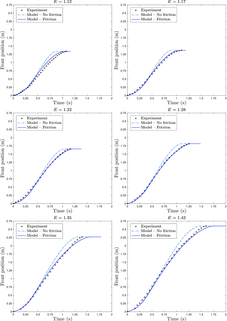
Figure 4.5. Flow kinematics: Temporal evolution of the frontal position for different initial expansions, from $12\%$ to $42\%$. Experimental results are represented by black crosses, numerical predictions with no basal friction are represented in light blue dashed lines, while those with an evolving basal friction given by $\kappa=R_{sed}/2$ are represented in dark blue continuous lines.

4.1. Kinematics of the flow fronts

We exposed in Figure 2.2 the typical kinematics curve of a dam-break flow, including its three main phases of transport. This characteristic profile is also shown in Figure 4.5 where we depict, for each of the six considered expansions, the evolution in time of the frontal position of the experimental flows (black crosses). For increasing expansions (from $E=1.12$ to $E=1.42$), the travelled distance of the flows significantly increases from about $1.25\ \mathrm{m}$ to more than $2.5\ \mathrm{m}$, while their duration increases from about $1.25\ \mathrm{s}$ to $2\ \mathrm{s}$. Furthermore, the profiles exhibit increasing fontal velocities during propagation, that can be better modeled with equations (3.10)–(3.14) (dark blue line).

The gravitational collapse. As the conditions for shallow water flows are not respected during this collapse phase, since the column height ($h{{}^{\mathrm{in}}}=0.27\ \mathrm{m}$) is much larger than its length ($x^{\mathrm{in}}=0.105\ \mathrm{m}$), we transferred the approach of Larrieu et al. [29] to our setting by letting the suspension sedimenting into a flowing layer of apparent height $x^{\mathrm{in}}/10$ at speed $(2gh)^{1/2}$ and during the time interval $[0,t_{ff}]$, where $t_{ff}\approx 0.23s$ denotes the representative free-fall time, which is encoded in the model through the source terms depending on $S_{slump}$ and is defined by (3.6). From Figure 4.5 we can see that this strategy allows us to well reproduce the accelerating behavior in each experiment and to capture, in particular, the correct initial frontal velocity at the beginning of the dominant phase of transport.

The sedimentation-dominated dynamics. A progressive sedimentation takes place in the dominant following phase of transport, where the suspension travels down the flume at constant speed. Despite the high Reynolds number of the flows, the sedimentation may develop independently in the Stokes flow regime where the effects of the fluid inertia are negligible, thus remaining similar to that measured in a static configuration [18, 19]. This means that taking $U_{sed}^{\mathsf{static}}$ from (2.1) as the reference settling velocity represents a reasonable simplification. In practice, we expect that the flow agitation could slightly influence this reference velocity, leading to the modeling assumption on the form of the sedimentation rate $R_{sed}$, that we recall here to be

$$R_{sed}=C(Re)\frac{\rho_{s}}{\rho_{s}-\rho_{f}}\frac{U_{sed}^{\mathsf{static}}}{\frac{\phi_{pack}}{\phi_{s}}-1},$$ (4.17)

as a function of $Re$. This parameter $R_{sed}$ governs the runout distance of the flow modeled by (3.10)–(3.14), and decreases with increasing expansions: the more the suspension is fluidized, the more agitation affects the vertical motion of particles, the more their sedimentation is delayed and thus the distance traveled by the flow is extended. Such feature is encoded here by the coefficient $C(Re)$, which encapsulates the effects of agitation within the suspension depending on the specific Reynolds number. Using $C(Re)$ as a free parameter in our model allows us to fit the runout distance of each experiment. A comparison between the kinematics profiles measured from the experiments (black crosses) and those predicted numerically is exposed in Figure 4.5 in cases where a basal friction at the interface with the deposit is included (dark blue continuous lines) or disregarded (light blue dashed lines). In particular, we fix $\kappa=R_{sed}/2$. We can notice that the model with $\kappa=0$ always underestimates the slope of the experimental profiles, justifying the use of friction for recovering the correct speed of propagation during this phase. This is confirmed by the good approximations provided by the curves in dark blue.

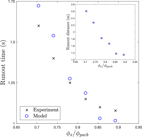
Figure 4.6. Runout time and distance: Duration and traveled distance of experimental flows (black crosses) as functions of the mixture concentration, as well as predictions gained from equations (3.10)–(3.14) by taking $\kappa=R_{sed}/2$ (blue circles).

The stopping phase. At the end of the flow, the suspension experiences a deceleration and motion ceases once all particles have settled, forming the final deposit. We observe in Figure 4.5 that all numerical profiles display a horizontal behavior at the end of the flow. This is related with the fact that once the front has stopped moving, the suspension located at the rear of the flow continues sedimenting on the top of the deposit and expelling water upward, as prescribed by the source terms that depend on $S_{sed}$ in equations (3.10)–(3.14). Conversely, the stopping phase of the experimental flows is characterized by two successive waves of motion: a first one corresponding to the propagation of the suspension which lasts until the front is at rest, and a second one associated with the remobilization of a small volume of suspension at the top of the deposit, forming a secondary front that transports the material forwards and extends the runout length of up to $8\%$ [16]. We speculate that this phenomenon is related to surface instabilities and is caused by a late fluidization (due to the pressure release after the deposit compaction) that develops at the rear part, which leads to a remobilization of a small volume of material and to its subsequent transport. In particular, the second wave is observed to be more significant for greater expansions, while its solid concentration progressively decreases with $E$. Since the present model is not designed to capture such secondary effects, we have chosen to reproduce the experimental kinematic profiles only up to the end of the first wave (meaning that we do not take into account the second wave in the experimental curves of Figure 4.5).

The drawback of this choice is a loss of precision in the model predictions for the flow duration, as shown by Figure 4.6. While the runout distances of the experimental flows are satisfyingly captured by the model, we can observe a discrepancy between the experimental and the predicted runout times, measured at the end of the first wave. This might be explained by the fact that we are not taking into account in equations (3.10)–(3.14) essential information about the dynamics of the second wave, making it difficult to identify the correct physical time and compare it with the numerical one.

4.2. Geometry of the final deposits

The secondary wave can be visualized a posteriori, by analyzing the deposit shapes and comparing them with the numerical predictions. The case of a volume expansion $E=1.28$ offers the best example. In Figure 4.7, we observe the final deposit measured experimentally (black crosses) and that obtained numerically from equations (3.10)–(3.14) (dark/light blue lines, with or without friction), highlighting through brown areas the volume transported by the secondary wave. We notice that the model fails to correctly reproduce the experimental deposit both at the rear and at the front, but the areas appear to compensate, so that the discrepancy may correspond to the remobilized material through the secondary wave (which is not included in the model). The latter flows over the deposit and transports particles forwards, explaining the differences between the predicted deposit geometry and the experimental one.

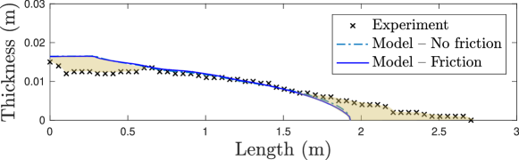
Figure 4.7. Second wave: Visualization of the second wave through its impact on the deposit geometry for $E=1.28$. The predicted excess of particles in the experimental deposit, represented in back, is comparable to that missing at the front (see brown colored areas).

We finally display in Figure 4.8 a similar comparison between experimental and numerical deposits, for the six values of $E$. As the expansion grows, the geometry of the measured deposits becomes more elongated and exhibits a more gentle slope, as well as a lower maximum thickness. This is due to the decrease of the sedimentation rate which acts in promoting the particles transport down the flume. We can also observe how the predictions from equations (3.10)–(3.14) provide more satisfying results for higher expansions, where the volume of particles remobilized by the secondary wave becomes negligible. Nevertheless, this secondary wave does not modify significantly the shape of the primary deposits, leading to global relevant numerical predictions.

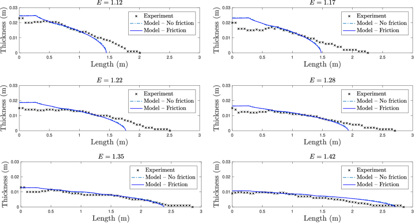
Figure 4.8. Final deposits: Geometry of the final deposits measured at the end of the experiments (black crosses). Comparison with the shapes predicted by the model, with or without basal friction (dark blue continuous line/light blue dashed line).

4.3. Limits of the model

We discuss now the main limitations of the model and the investigations that we plan to carry out in the near future to solve them. These latter involve the measurement of the internal flow structure (namely, the velocity fields) to take into account the development of a basal boundary layer, as well as the modeling strategy to describe the secondary wave after the stop of the primary one.

Statical and dynamical sedimentation velocities. We presented a general law (2.1) which describes the sedimentation velocity $U_{sed}^{\mathsf{static}}$ of solid particles in a low-inertia fluid (gas or water) in static suspensions [17, 1]. This law provides a correction to the theoretical Stokes velocity of a single particle of density $\rho_{s}$, with no inertia ($St_{0}=0$) and falling in a high-viscosity fluid ($Re=0$, in the Stokes flow regime) at rest, by taking into account the mixture density $\rho_{m}$ (through the factor $1-\phi_{s}$) and the mixture viscosity $\mu_{m}$ (through the effect of the particle concentration $\mathcal{F}_{1}(\phi_{s}/\phi_{pack})$ and of the particle inertia $\mathcal{F}_{2}(St_{0})$), which act respectively on the buoyancy force and on the drag force applied to each particle.

In this work, we focused our attention on the sedimentation process developed in flowing suspensions. Comparisons of the settling velocities $U_{sed}^{\mathsf{static}}$ measured in static configurations with those predicted in flowing suspensions $U_{sed}^{\mathsf{dynamic}}$ have highlighted that, from a critical value $Re_{c}=250$ of the Reynolds number $Re\geq Re_{c}$, the flow becomes agitated enough to disturb the vertical motion of the particles and to delay their settling velocity. This effect is taken into account in our model through the coefficients $C(Re)$, that can be approximated by a function $\mathcal{F}_{3}(Re)$ of the form

$$\mathcal{F}_{3}(x)=\frac{0.53}{0.53+e^{0.06(x-2Re_{c})}},$$ (4.18)

which decreases with $Re$ and thus with decreasing mixture concentrations (see Figure 4.9). This means that, when $Re\leq Re_{c}$, the suspension dynamics can be described as a low-viscosity quasi-parallel flow [18] with no significant vertical velocity fluctuations capable of disturbing the falling motion of particles, and therefore $C(Re)\approx 1$. Above this threshold value, fluctuating eddies are likely to develop at the scale of the particles, which may significantly delay their sedimentation. Therefore, additional studies are required to analyze these aspects related to mixtures agitation.

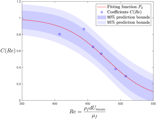
Figure 4.9. Fitting of $C(Re)$ with $\mathcal{F}_{3}$: Best fit of the coefficients $C(Re)$, describing the delay of particles sedimentation velocity due to mixture agitation. The fitting function is given by (4.18) and is plotted along with the corresponding $80\%$ and $95\%$ prediction bounds.

Modeling the secondary wave. We saw that the model is able to reproduce the relevant kinematic evolution of the flow front, for dam-break particulate suspensions initially fully fluidized, as well as their final deposits. It appears however that the model loses precision when predicting the runout duration of the flows and their deposits for low expansion rates, as shown in Figure 4.5 and Figure 4.8 respectively. This can be explained by the presence of a secondary wave of flowing material, observed experimentally, that arises at the surface of the main deposits (from the gas loss induced by their compaction, causing a late fluidization of the surface layer once the general motion has ceased) and continues propagating briefly, thus elongating the final runout lengths and deposits. These phenomena requires more sophisticated multi-dimensional and multi-phase approaches to be captured, which are out of the scope of the present paper, since our primary objective was to capture the mean flows features using a very simple mathematical description, associated with a low computational complexity, that could also constitute a relevant framework for large-scale simulations of natural flows traveling down real topographies.

5. Conclusions

In this work, we conducted laboratory experiments of the dam-break flows of homogeneous suspensions of different concentrations, made of non-cohesive glass beads and water, whose dynamics is mostly dominated by sedimentation. Starting from a coupled Euler–Navier–Stokes formulation, we derived a simple three-layer depth-integrated shallow water model to describe the flows evolution and their deposits. The resulting system of equations includes three source terms built to model respectively the column collapse (during the initial non shallow water phase), the propagation velocity of the suspension front and the sedimentation process that leads to the basal deposit. The first term is obtained through an adaptation of the method of [29] for granular collapses and describes the gravitational slumping as the particles free-fall into a moving apparent thin layer. The second one is given by a laminar-type basal friction for the suspension layer when traveling above the deposit, and is taken proportional to the settling velocity [43]. The last one translates the particles sedimentation rate in flowing suspensions, inferred from the experiments and the model. The next step will be to determine an empirical law for the evolution of these coefficients as a function of the flow Reynolds number, to highlight that the particle deposition can be affected by the flow agitation above a threshold value of $Re$. The equations were solved numerically using a splitting strategy based on a hydrostatic upwind scheme that allows to treat the system in an uncoupled way [5], while the evolution of each layer is separately approximated through a finite volume scheme that uses the HLL solver for the numerical fluxes. The proposed model allows to recover the first order frontal kinematic profiles as well as the deposits geometry, and to capture in particular the relevant flow front velocity after the slumping phase. The development of a secondary wave at the end the flow slightly alter the reproduction of the accurate deposits shape. A possible way to incorporate this effect may be to consider a more elaborated two-phase flow formulation with a time-evolving volume fraction $\phi_{s}$ [35, 8, 4]. These investigations are left for future developments.

Acknowledgements. This study was supported by the Region Centre-Val de Loire through the Contribution of the “Academic Initiative” RHEFLEXES/2019-00134935. A.B. also acknowledges the support from the Austrian Science Fund (FWF), within the Lise Meitner project No. M-3007 (Asymptotic Derivation of Diffusion Models for Mixtures), and from the European Union’s Horizon Europe research and innovation programme, under the Marie Sklodowska-Curie grant agreement No. 101110920 (MesoCroMo - A Mesoscopic approach to Cross-diffusion Modelling in population dynamics).

Appendix A Derivation of the interfaces’ equations

In this first appendix, we focus our attention on the derivation of equations (3.8)–(3.10), describing the evolution of the interfaces that separates the three layers of the flow. Let us take $t>t_{ff}$, where $t_{ff}$ is the critical time (3.7) starting from which these three interfaces form. We begin by considering a fixed control volume $\Omega$ around the three interfaces, as well as four mobile domains that we call $\Omega_{d}^{t}$ for the deposit, $\Omega_{m}^{t}$ for the grains–water mixture, $\Omega_{f}^{t}$ for the pure fluid and $\Omega_{\textrm{air}}^{t}$ for the upper ambient air (see Figure 1.10). Then, assuming incompressibility holds, we may write the continuity equation for the two-dimensional flow inside each layer in the general non-conservative form

$$\partial_{t}\rho+\rho\partial_{x}u+\partial_{z}w=0,$$ (1.19)

where the inhomogeneity of the medium is encoded by a piecewise constant (constant in each of the four domains $\Omega_{d}^{t}$, $\Omega_{m}^{t}$, $\Omega_{f}^{t}$ and $\Omega_{\textrm{air}}^{t}$) density $\rho$ and by a piecewise regular (similarly, regular in each of the four domains) velocity field $v=\left(\begin{array}[]{c}u\\ w\end{array}\right)$, with $u$ and $w$ denoting the horizontal and vertical velocity components respectively. In particular, we characterize the explicit form of the density $\rho$ and of the mass flux $\rho v$ inside the four layers in the following way.

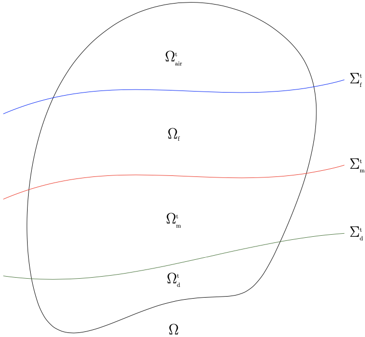
Figure 1.10. Control volume: Sketch of the control volume $\Omega^{t}$ used to determine the evolution equations for the interfaces.

The deposit is characterized by a particles’ volume fraction $\phi_{pack}$, therefore inside $\Omega_{d}$ we have that $\rho$ is given by the effective density $\rho_{d}=\phi_{pack}\rho_{s}+(1-\phi_{pack})\rho_{f}$. Since we have assumed that the particles stop moving when they settle down, it is also natural to consider a zero mass flux $\rho v$ inside the deposit, i.e. we take $\rho v_{d}=\rho_{d}\left(\begin{array}[]{c}0\\ 0\end{array}\right)$. Next, the solid volume fraction associated with the suspension is $\phi_{s}$, and thus the effective density inside $\Omega_{m}$ is given by $\rho_{m}=\phi_{s}\rho_{s}+(1-\phi_{s})\rho_{f}$. Moreover, we assume that the sedimentation of particles onto the underlying deposit takes place in this layer solely in the vertical direction, oriented downward, with a velocity $-U_{sed}^{\mathsf{dynamic}}$. Since the velocity field in non-zero here, we need to account for both the fluid’s and the particles’ velocities. Therefore, we may write the mass flux inside the suspension as $\rho v_{m}=\phi_{s}\rho_{s}\left(\begin{array}[]{c}u\\ w-U_{sed}^{\mathsf{dynamic}}\end{array}\right)+(1-\phi_{s})\rho_{f}\left(\begin{array}[]{c}u\\ w\end{array}\right)$. At last, there are no particles inside the fluid and the ambient air layers, and thus $\Omega_{f}$ and $\Omega_{\textrm{air}}$ can be simply characterized by the densities $\rho_{f}$ and $\rho_{\textrm{air}}$, respectively, and by the mass fluxes $\rho v_{f}=\rho_{f}\left(\begin{array}[]{c}U\\ W\end{array}\right)$ and $\rho v_{\textrm{air}}=\rho_{\textrm{air}}\left(\begin{array}[]{c}u\\ w\end{array}\right)$. Notice that $\rho_{\textrm{air}}\ll\rho_{f}$ and that, in order to avoid any confusion between the velocity of the fluid inside the domains $\Omega_{f}$ and $\Omega_{m}$, we have used the uppercase letters $U$ and $V$ to denote the water’s velocity field in the upper pure fluid layer and the lowercase letters $u$ and $v$ to denote its counterpart in the suspension layer.

Introducing now the vector of moments $J=\left(\begin{array}[]{c}\rho\\ \rho v\end{array}\right)$, we can rewrite the continuity equation (1.19) in a more compact form as $\nabla_{(t,x,z)}\cdot J=0$. Given any test function $\psi:\Omega\to\mathbb{R}\in C_{c}^{1}(\Omega)$, we then pass to a weak formulation of the latter to obtain

$$\int_{\Omega}J\cdot\nabla_{(t,x,z)}\psi\mathrm{d}\Omega=0,$$

and an application of Stokes–Ostrogradsky theorem starting from the divergence of $\psi J$ over $\Omega$ leads to the relation

$$\int_{\Sigma}\psi J\cdot\textbf{n}\mathrm{d}\Sigma=0,$$ (1.20)

where we denote with a general $\Sigma$ the surface identified by the compact support of $\psi$ inside $\Omega$ and with $\mathbf{n}$ the outward normal vector to this boundary. The idea is to study each interface separately using these tools. For the interface $\Sigma_{d}^{t}$ between the deposit and the suspension, identified by the height $h_{d}(t,x)$, one may reduce the support of $\psi$ around $\Sigma_{d}^{t}$ so that we can rule out the influence of the other two interfaces and transform (1.20) into the equivalence

$$\int_{\Sigma_{d}^{t}}\psi J_{m}\cdot\mathbf{n}_{d}\mathrm{d}\Sigma_{d}^{t}-\int_{\Sigma_{d}^{t}}\psi J_{d}\cdot\mathbf{n}_{d}\mathrm{d}\Sigma_{d}^{t}=0,$$

where $\displaystyle\mathbf{n}_{d}=\frac{1}{\sqrt{1+|\partial_{x}h_{d}|^{2}+|\partial_{t}h_{d}|^{2}}}\left(\begin{array}[]{c}\partial_{t}h_{d}\\ \partial_{x}h_{d}\\ -1\end{array}\right)$ is the outward normal vector to $\Sigma_{d}^{t}$, directed from $\Omega_{d}^{t}$ to $\Omega_{m}^{t}$. Choosing a suitable mollified step function $\psi$ such that $\psi\equiv 1$ on $\Sigma_{d}^{t}$, we can finally replace $J_{m}$ and $J_{d}$ with their explicit values to get

$$(\rho_{m}-\rho_{d})\partial_{t}h_{d}+\rho_{m}u|_{z=h_{d}}\partial_{x}h_{d}-\rho_{m}w|_{z=h_{d}}=-\phi_{s}\rho_{s}U_{sed}^{\mathsf{dynamic}}.$$

But $\rho_{m}-\rho_{d}=(\phi_{s}-\phi_{pack})(\rho_{s}-\rho_{f})$ and simple algebraic manipulations lead to

$$\partial_{t}h_{d}+\frac{\rho_{m}}{\rho_{s}-\rho_{f}}\frac{1}{\phi_{s}-\phi_{pack}}\left(u|_{z=h_{d}}\partial_{x}h_{d}-w|_{z=h_{d}}\right)=R_{sed}.$$

By assuming the non-penetration condition $u|_{z=h_{d}}\partial_{x}h_{d}=w|_{z=h_{d}}$ and recalling that $S_{sed}(t)=R_{sed}\chi(t>t_{ff})$, we finally recover equation (3.10) giving the evolution of the deposit’s interface $\Sigma_{d}^{t}$ in terms of the height $h_{d}$. Obviously, the same reasoning can be applied to deal with the other two interfaces and recover equations (3.8)–(3.9), by reducing relation (1.20) to $\Sigma_{m}^{t}$ and $\Sigma_{f}^{t}$ respectively and by using the definitions of $J_{m}$ and $J_{f}$, as done for $\Sigma_{d}^{t}$ and $J_{m}$, $J_{d}$. The only difference in these two cases is that we do not need to impose a non-penetration condition as for the interface $\Sigma_{d}^{t}$. Moreover, since $\rho_{\textrm{air}}\ll\rho_{f}$ it is natural to take $\rho_{f}-\rho_{\textrm{air}}\approx\rho_{f}$ when writing the spatio-temporal evolution of $\Sigma_{f}^{t}$ (this is the reason why we do not see the explicit appearance of the density $\rho_{\textrm{air}}$ in equation (3.8), since the differences $\rho_{f}-\rho_{\textrm{air}}$ have been simply replaced by $\rho_{f}$).

Appendix B Derivation of the two-layer shallow water system

This second part is dedicated to the derivation of our model (3.11)–(3.14). Notice that we still focus on the case when $t>t_{ff}$, since we have assumed that no sedimentation takes place before this critical time and the shallow water system (3.5) accounting for the slumping phase has already been derived and extensively studied in previous works [29, 14]. Starting from the assumptions presented in Section 3, the main idea is to set up Euler- and Navier–Stokes-type equations to describe the evolution of the fluid and suspension layers respectively, and then derive in a suitable thin-layer approximation the expected shallow water system by depth-averaging the equations. Our derivation will follow similar steps and assumptions from the work of Gerbeau and Perthame [15], and is also close in its reasoning to the earlier work of Liu and Mei for Bingham plastic fluids [31]. In what follows, we shall always use the convention that lowercase letters refer to quantities of the suspension layer, while capital letters refer to quantities of the fluid one. In particular, we introduce the horizontal $u=t(t,x,z)$ and vertical $w=w(t,x,z)$ components of the velocity field inside the suspension layer, together with their counterparts $U=U(t,x,z)$ and $W=W(t,x,z)$ inside the fluid layer. Moreover, recall that each of the two layers is contained between two interfaces, identified by lateral heights. In particular, the suspension layer spans from $h_{d}$ to $h_{m}$, while the fluid one spans from $h_{m}$ to $h_{f}$.

Then, the Euler system describing the evolution of the perfect fluid layer writes as

$$\partial_{x}U+\partial_{z}W=0,$$

$$\rho_{f}(\partial_{t}U+U\partial_{x}U+W\partial_{z}U)=-\partial_{x}P,$$ (2.21)

$$\rho_{f}(\partial_{t}W+U\partial_{x}W+W\partial_{z}W)=-\partial_{z}P-\rho_{f}g,$$

while the suspension layer evolves following the Navier–Stokes system

$$\partial_{x}u+\partial_{z}w=0,$$

$$\rho_{m}(\partial_{t}u+u\partial_{x}u+w\partial_{z}u)=-\partial_{x}p+2\mu_{m}\partial_{x}^{2}u+\mu_{m}\partial_{zx}^{2}w+\mu_{m}\partial_{z}^{2}u,$$ (2.22)

$$\rho_{m}(\partial_{t}w+u\partial_{x}w+w\partial_{z}w)=-\partial_{z}p-\rho_{m}g+\mu_{m}\partial_{xz}^{2}u+\mu_{m}\partial_{x}^{2}w+2\mu_{m}\partial_{z}^{2}w.$$

In the above equations, the quantities $P=P(t,x,z)$ and $p=p(t,x,z)$ denote the respective layers’ pressures, while $\mu_{m}$ defines the dynamic viscosity of the suspension. In particular, we may write $\mu_{m}=\rho_{m}\nu_{m}$, with $\nu_{m}$ defining the associated suspension’s kinematic viscosity. We stress here that this kind of approximation is reminiscent of the one proposed by Liu and Mei [31] to model Bingham-type rheologies. Here, the distinction between layers stems from the use of two different densities $\rho_{f}$ and $\rho_{m}$, instead of two separate viscosities.

We complete the coupled systems (2.21)–(2.22) with the equations governing the three interfaces (3.8)–(3.10) and with the following boundary conditions. At the interface with the deposit, we impose the Navier condition

$$\left(\kappa u-\mu_{m}\partial_{z}u\right)|_{z=h_{d}}=0,$$ (2.23)

and the non-penetration condition

$$u|_{z=h_{d}}\partial_{x}h_{d}-w|_{z=h_{d}}=0.$$ (2.24)

Next, we assume continuity of the pressure and of the shear rate at the interface between suspension and fluid, namely

$$p|_{z=h_{m}}=P|_{z=h_{m}},\qquad\partial_{z}u|_{z=h_{m}}=\partial_{z}U|_{z=h_{m}},$$ (2.25)

and we further impose the non-penetration condition

$$u|_{z=h_{m}}\partial_{x}h_{m}-w|_{z=h_{m}}=U|_{z=h_{m}}\partial_{x}h_{m}-W|_{z=h_{m}}.$$ (2.26)

Finally, at the upper interface between the fluid and the ambient air we impose the stress-free boundary condition

$$(\sigma-P\mathbb{I}_{2})\cdot\mathbf{n}_{f}=0,\quad\textrm{at }z=h_{f},$$ (2.27)

where $\sigma=\sigma(t,x,z)$ denotes the perfect fluid’s deviatoric stress tensor

$$\sigma=\left(\begin{array}[]{cc}2\partial_{x}U&\partial_{x}W+\partial_{z}U\\[5.69054pt] \partial_{x}W+\partial_{z}U&2\partial_{z}W\end{array}\right),$$

the vector $\mathbf{n}_{f}$ denotes the outward normal at $z=h_{f}$, namely

$$\mathbf{n}_{f}=\frac{1}{\sqrt{1+|\partial_{x}h_{f}|^{2}}}\left(\begin{array}[]{c}-\partial_{x}h_{f}\\[5.69054pt] 1\end{array}\right),$$

and $\mathbb{I}_{2}$ is the identity matrix in two dimensions.

We proceed to determine the corresponding nondimensionalized form of the previous equations, by looking at a thin-layer regime of small ratio $\varepsilon=\frac{h_{0}}{L_{0}}\ll 1$, where $h_{0}$ and $L_{0}$ denote respectively a characteristic height and length of the flow domain. Let us also introduce a characteristic speed $u_{0}$ of the flow and a unitary measure of dynamic viscosity $\mu$. Then, we consider the following rescaling of our relevant physical quantities

$$x=L_{0}x^{*},\quad z=h_{0}z^{*},\quad t=\frac{L_{0}}{u_{0}}t^{*},\quad h_{d}=h_{0}h_{d}^{*},\quad h_{m}=h_{0}h_{m}^{*},\quad h_{f}=h_{0}h_{f}^{*},$$

$$u=u_{0}u^{*},\quad U=u_{0}U^{*},\quad w=\varepsilon u_{0}w^{*},\quad W=\varepsilon u_{0}W^{*},\quad U_{sed}^{\mathsf{dynamic}}=\varepsilon u_{0}U_{sed}^{*},$$

$$p=\rho_{m}gh_{0}p^{*},\quad P=\rho_{f}gh_{0}P^{*},\quad\sigma=\mu\frac{u_{0}}{h_{0}}\sigma^{*},\quad\kappa=\rho_{m}\varepsilon u_{0}\kappa^{*},$$

and we use the definitions $Re_{m}=\frac{h_{0}u_{0}}{\nu_{m}}$ and $Fr=\frac{u_{0}}{\sqrt{gh_{0}}}$ for the Reynolds and Froude numbers of the flow. Notice that the term $\kappa u$ has the correct dimension of a friction and its rescaling is coherent with our choice of $\kappa$, since $\kappa/\rho_{m}\approx U_{sed}^{\mathsf{dynamic}}=\varepsilon u_{0}U_{sed}^{*}$. The latter rescaling of the basal friction corresponds in particular to the one proposed in [15].

By switching to the above nondimensional variables and by doing simple algebraic manipulations, the fluid layer’s evolution system (2.21) rewrites

$$\partial_{x}U+\partial_{z}W=0,$$

$$\partial_{t}U+U\partial_{x}U+W\partial_{z}U=-\frac{1}{Fr^{2}}\partial_{x}P,$$

$$\varepsilon^{2}(\partial_{t}W+U\partial_{x}W+W\partial_{z}W)=-\frac{1}{Fr^{2}}\partial_{z}P-\frac{1}{Fr^{2}},$$

where we have dropped the starred notation for convenience. Similarly, starting from (2.22), the nondimensionalized system governing the evolution of the suspension layer takes the form

$$\partial_{x}u+\partial_{z}w=0,$$

$$\partial_{t}u+u\partial_{x}u+w\partial_{z}u=-\frac{1}{Fr^{2}}\partial_{x}p+\frac{2\varepsilon}{Re_{m}}\partial_{x}^{2}u+\frac{\varepsilon}{Re_{m}}\partial_{zx}^{2}w+\frac{1}{\varepsilon Re_{m}}\partial_{z}^{2}u,$$

$$\varepsilon^{2}(\partial_{t}w+u\partial_{x}w+w\partial_{z}w)=-\frac{1}{Fr^{2}}\partial_{z}p-\frac{1}{Fr^{2}}+\frac{\varepsilon}{Re_{m}}\partial_{xz}^{2}u+\frac{\varepsilon^{3}}{Re_{m}}\partial_{x}^{2}w+\frac{2\varepsilon^{2}}{Re_{m}}\partial_{z}^{2}w.$$

Next, the structure of the equations for the three interfaces (3.8)–(3.10) does not modify when passing to nondimensional quantities. The Navier condition (2.23) then rewrites as

$$\varepsilon\kappa u-\frac{1}{Re_{m}}\partial_{z}u=0,\quad\textrm{at }z=h_{d},$$ (2.28)

while the non-penetration condition (2.24) is left untouched by the rescaling. The same consideration obviously holds for the other non-penetration relation (2.26) at $z=h_{m}$. We continue with the continuity conditions (2.29) for pressure and shear rate at the suspension-fluid interface, which lead to the following nondimensional relations:

$$\rho_{m}p|_{z=h_{m}}=\rho_{f}P|_{z=h_{m}},\qquad\partial_{z}u|_{z=h_{m}}=\partial_{z}U|_{z=h_{m}}.$$ (2.29)

At last, the rescaling of the stress-free condition (2.27) at the fluid-air interface leads to the relations

$$\partial_{z}U=\left(2\varepsilon^{2}\partial_{x}U-\varepsilon P\right)\partial_{x}h_{f}-\varepsilon^{2}\partial_{x}W,\quad\textrm{at }z=h_{f},$$

and

$$P=2\varepsilon\partial_{z}W-\varepsilon\left(\varepsilon^{2}\partial_{x}W+\partial_{z}U\right)\partial_{x}h_{f},\quad\textrm{at }z=h_{f}.$$

Now, by collecting every term of lower order in $\varepsilon$ in the previous rescaled equations and in the boundary conditions, we end up with an asymptotic regime where the fluid layer evolves through the system

$$\partial_{x}U+\partial_{z}W=0,$$ (2.30)

$$\partial_{t}U+U\partial_{x}U+W\partial_{z}U=-\frac{1}{Fr^{2}}\partial_{x}P,$$ (2.31)

$$\partial_{z}P+1=\mathcal{O}(\varepsilon^{2}),$$ (2.32)

while for the system governing the evolution of the suspension layer we recover the approximation

$$\partial_{x}u+\partial_{z}w=0,$$ (2.33)

$$\partial_{t}u+u\partial_{x}u+w\partial_{z}u=-\frac{1}{Fr^{2}}\partial_{x}p+\frac{1}{\varepsilon Re_{m}}\partial_{z}^{2}u+\mathcal{O}(\varepsilon),$$ (2.34)

$$\partial_{z}p+1=\mathcal{O}(\varepsilon).$$ (2.35)

The Navier condition along the top of the deposit carries over keeping the same structure and the same holds for the non-penetration condition (2.26) and the continuity of pressure and shear stress (2.29) at $z=h_{m}$.

The stress-free condition at the upper surface then provides the approximations

$$\partial_{z}U=\mathcal{O}(\varepsilon^{2}),\quad\textrm{at }z=h_{f},$$ (2.36)

$$P=\mathcal{O}(\varepsilon),\quad\textrm{at }z=h_{f}.$$ (2.37)

At last, recall that the equations for the evolving interfaces are not modified in the rescaling and thus correspond to the original ones (3.8)–(3.10).

Starting from this asymptotic regime, the procedure for deriving the corresponding shallow water equations is standard. First of all, the hydrostatic relation (2.32) tells us that the pressure $P$ does not depend on $x$ up to order $\mathcal{O}(\varepsilon^{2})$. Therefore, from the conservation equation for the vertical velocity (2.31) and from the approximation (2.36) at $z=h_{f}$ we deduce that $\partial_{z}U=\mathcal{O}(\varepsilon^{2})$ inside the whole fluid layer (and in particular at its lower interface $z=h_{m}$). Next, multiplying by $\varepsilon$ both sides of equation (2.34), we find that $\partial_{z}^{2}u=\mathcal{O}(\varepsilon)$. Moreover, the Navier condition (2.28) implies that $\partial_{z}u|_{z=h_{d}}=\mathcal{O}(\varepsilon)$, while the transmission condition for the shear stress (2.29) across $z=h_{m}$ gives $\partial_{z}u|_{z=h_{m}}=\mathcal{O}(\varepsilon^{2})$. All these considerations allow to finally infer that the flow behaves like a plug in both the fluid and the suspension layers, and does not depend on $z$ at the leading order in $\varepsilon^{2}$ and $\varepsilon$ respectively. In particular, we deduce the existence of two velocities $\overline{U}=\overline{U}(t,x)$ and $\overline{u}=\overline{u}(t,x)$ such that

$$U(t,x,z)=\overline{U}(t,x)+\mathcal{O}(\varepsilon^{2}),\quad u(t,x,z)=\overline{u}(t,x)+\mathcal{O}(\varepsilon).$$ (2.38)

We now proceed by integrating in $z$ over $[h_{m},h_{f}]$ the fluid’s incompressibility condition (2.30) and we apply Leibniz integral rule to recover

$$\partial_{x}\int_{h_{m}}^{h_{f}}U(t,x,z)\mathrm{d}z-U|_{z=h_{f}}\partial_{x}h_{f}+W|_{z=h_{f}}+U|_{z=h_{m}}\partial_{x}h_{m}-W|_{z=h_{m}}=0.$$

Using the equations (3.8)–(3.9) for the interfaces $\Sigma_{f}^{t}$ and $\Sigma_{m}^{t}$, together with the non-penetration condition (2.26), we thus recover the mass conservation equation for the fluid layer

$$\partial_{t}H+\partial_{x}(H\bar{U})=\left(\frac{\phi_{pack}}{\phi_{s}}-1\right)R_{sed},$$

where we have defined the height of the fluid layer $H=h_{f}-h_{m}$, which simply implies that $\int_{h_{m}}^{h_{f}}U(t,x,z)\mathrm{d}z=H\bar{U}$ at the leading order. Taking the limit $\varepsilon\to 0$ in the hydrostatic relation (2.32) and integrating over $[z,h_{f}]$, we then use the boundary condition (2.37) for $P$ at $z=h_{f}$ to infer the explicit form of the pressure in the fluid layer, which reads

$$P(t,x,z) =h_{f}-z=H+h+h_{d}-z,\quad z\in[h_{m},h_{f}].$$

where we have further defined the height of the suspension layer $h=h_{m}-h_{d}$. In particular, we find that $\partial_{x}P=\partial_{x}h_{f}=\partial_{x}(H+h+h_{d})$. Therefore, one proceed by integrating in $z$ over $[h_{m},h_{f}]$ the equation for the conservation of horizontal velocity (2.31) to initially obtain

$$\int_{h_{m}}^{h_{f}}\partial_{t}U\mathrm{d}z+\int_{h_{m}}^{h_{f}}2U\partial_{x}U\mathrm{d}z+U|_{z=h_{f}}W|_{z=h_{f}}-U|_{z=h_{m}}W|_{z=h_{m}}=-\frac{1}{Fr^{2}}H\partial_{x}(H+h+h_{d}),$$

where we have integrated by parts the nonlinear term $W\partial_{z}U$ and used the incompressibility condition (2.30) to see that $\partial_{z}W=-\partial_{x}U$. By now applying Leibniz integral rule to both the temporal derivative $\partial_{t}U$ and the nonlinear term $2U\partial_{x}U$, we then recover

$$\partial_{t}\int_{h_{m}}^{h_{f}}U(t,x,z)\mathrm{d}z+\partial_{x}\int_{h_{m}}^{h_{f}}U^{2}(t,x,z)\mathrm{d}z-U|_{z=h_{f}}\left(\partial_{t}h_{f}+U|_{z=h_{f}}\partial_{x}h_{f}-W|_{z=h_{f}}\right)\\[11.38109pt] +U|_{z=h_{m}}\left(\partial_{t}h_{m}+U|_{z=h_{m}}\partial_{x}h_{m}-W|_{z=h_{m}}\right)=-\frac{1}{Fr^{2}}H\partial_{x}(H+h+h_{d}),$$

which finally provides the momentum conservation equation for the fluid layer (going back to dimensional variables)

$$\partial_{t}(H\bar{U})+\partial_{x}(H\bar{U}^{2})=\left(\frac{\phi_{pack}}{\phi_{s}}-1\right)R_{sed}\bar{U}-gH\partial_{x}(H+h+h_{d}),$$

by replacing the expressions for the interfaces’ equations (3.8)–(3.9), combined with the non-penetration condition (2.26) at $z=h_{m}$, and by using the expansion (2.38) for $U$ which tells us that

$$\int_{h_{m}}^{h_{f}}U^{2}(t,x,z)\mathrm{d}z=H\bar{U}^{2},\quad U|_{z=h_{f}}=U|_{z=h_{m}}=\bar{U},$$

We continue with the analysis of the asymptotic system governing the suspension layer. We start by integrating in $z$ over $[h_{d},h_{m}]$ the incompressibility relation (2.33) and using Leibniz rule as before to get

$$\partial_{x}\int_{h_{d}}^{h_{m}}u(t,x,z)\mathrm{d}z-u|_{z=h_{m}}\partial_{x}h_{m}+w|_{z=h_{m}}+u|_{z=h_{d}}\partial_{x}h_{d}-w|_{z=h_{d}}=0,$$

from which we easily derive the mass conservation equation for the suspension layer

$$\partial_{t}h+\partial_{x}(h\bar{u})=-\frac{\phi_{pack}}{\phi_{s}}R_{sed},$$

by using the equations (3.9)–(3.10) for the interfaces $\Sigma_{m}^{t}$ and $\Sigma_{d}^{t}$, and by recalling the definition $h=h_{m}-h_{d}$, so that the expansion (2.38) leads to $\int_{h_{d}}^{h_{m}}u(t,x,z)\mathrm{d}z=h\bar{u}$. We then consider the hydrostatic relation (2.35) and integrate it over $[z,h_{m}]$ to exploit the transmission condition for the pressure (2.29) across the interface $\Sigma_{m}^{t}$ to find an explicit expression for $p$, namely

$$p(t,x,z) =\frac{\rho_{f}(h_{f}-h_{m})+\rho_{m}(h_{m}-z)}{\rho_{m}}=\frac{\rho_{f}}{\rho_{m}}H+h+h_{d}-z,\quad z\in[h_{m},h_{f}].$$

Once again, from the above we infer that $\partial_{x}p=\partial_{x}\left(\frac{\rho_{f}}{\rho_{m}}H+h+h_{d}\right)$, and this relation can be injected in the conservation equation for the suspension’s horizontal velocity (2.34) to recover, after integration in $z$ over $[h_{d},h_{m}]$, the initial approximation

$$\int_{h_{d}}^{h_{m}}\partial_{t}u\mathrm{d}z+\int_{h_{d}}^{h_{m}}u\partial_{x}u\mathrm{d}z+\int_{h_{d}}^{h_{m}}w\partial_{z}u\mathrm{d}z=-\frac{1}{Fr^{2}}h\partial_{x}\left(\frac{\rho_{f}}{\rho_{m}}H+h+h_{d}\right)+\frac{1}{\varepsilon Re_{m}}\int_{h_{d}}^{h_{m}}\partial_{z}^{2}u\mathrm{d}z+\mathcal{O}(\varepsilon).$$

Now, from the Navier condition (2.28) and the continuity of the shear rate (2.29) at $z=h_{m}$, we infer that

$$\frac{1}{\varepsilon Re_{m}}\int_{h_{d}}^{h_{m}}\partial_{z}^{2}u\mathrm{d}z=-\kappa u|_{z=h_{d}}+\mathcal{O}(\varepsilon),$$

and we proceed with the same calculations used previously for the fluid layer, to end up with the following equation:

$$\partial_{t}\int_{h_{d}}^{h_{m}}u(t,x,z)\mathrm{d}z+\partial_{x}\int_{h_{d}}^{h_{m}}u^{2}(t,x,z)\mathrm{d}z-u|_{z=h_{m}}\left(\partial_{t}h_{m}+u|_{z=h_{m}}\partial_{x}h_{m}-w|_{z=h_{m}}\right)\\[11.38109pt] +u|_{z=h_{d}}\left(\partial_{t}h_{d}+u|_{z=h_{d}}\partial_{x}h_{d}-w|_{z=h_{d}}\right)=-\frac{1}{Fr^{2}}h\partial_{x}\left(\frac{\rho_{f}}{\rho_{m}}H+h+h_{d}\right)-\kappa u|_{z=h_{d}}+\mathcal{O}(\varepsilon).$$

From this approximation, one finally deduces the momentum conservation equation (in dimensional form) for the suspension layer

$$\partial_{t}(h\bar{u})+\partial_{x}(h\bar{u}^{2})=-\frac{\phi_{pack}}{\phi_{s}}R_{sed}\bar{u}-\kappa\bar{u}-gh\partial_{x}\left(\frac{\rho_{f}}{\rho_{s}}H+h+h_{d}\right),$$

where we have replaced the expressions for the interfaces’ equations (3.9)–(3.10), together with the non-penetration condition (2.24) at $z=h_{d}$ to get rid of the term $u|_{z=h_{d}}\partial_{x}h_{d}-w|_{z=h_{d}}$, and used once again the expansion (2.38) for $u$ to see that

$$\int_{h_{d}}^{h_{m}}u^{2}(t,x,z)\mathrm{d}z=h\bar{u}^{2},\quad u|_{z=h_{m}}=u|_{z=h_{d}}=\bar{u}.$$

References

- [1] A. Amin, L. Girolami, and F. Risso. On the fluidization/sedimentation velocity of a homogeneous suspension in a low-inertia fluid. Powder Technol., 391:1–10, 2021.
- [2] R. Artoni, A. Santomaso, F. Gabrieli, D. Tono, and S. Cola. Collapse of quasi-two-dimensional wet granular columns. Phys. Rev. E, 87:032205, 2013.
- [3] E. Audusse. A multilayer Saint-Venant model: Derivation and numerical validation. Discrete Contin. Dyn. Syst. Ser. B, 5:189–214, 2005.
- [4] A. Baumgarten and K. Kamrin. A general fluid-sediment mixture model and constitutive theory validated in many flow regimes. J. Fluid Mech., 861:721–764, 2019.
- [5] C. Berthon, F. Foucher, and T. Morales. An efficient splitting technique for two-layer shallow-water model. Numer. Methods Partial Differential Equations, 31:1396–1423, 2015.
- [6] F. Bouchut. Nonlinear stability of finite volume methods for hyperbolic conservation laws and well-balanced schemes for sources. Frontiers in Mathematics. Birkhäuser Verlag, Basel, 2004.
- [7] F. Bouchut, E. D. Fernández-Nieto, A. Mangeney, and G. Narbona-Reina. A two-phase shallow debris flow model with energy balance. ESAIM: M2AN, 49:101–140, 2015.
- [8] F. Bouchut, E. D. Fernández-Nieto, A. Mangeney, and G. Narbona-Reina. A two-phase two-layer model for fluidized granular flows with dilatancy effects. J. Fluid Mech., 801:166–221, 2016.
- [9] F. Bouchut and T. Morales de Luna. An entropy satisfying scheme for two-layer shallow water equations with uncoupled treatment. M2AN Math. Model. Numer. Anal., 42:683–698, 2008.
- [10] A. Bougouin, L. Lacaze, and T. Bonometti. Collapse of a liquid-saturated granular column on a horizontal plane. Phys. Rev. Fluids, 4:124306, 2019.
- [11] P. Brufau, P. Garcia-Navarro, P. Ghilardi, L. Natale, and F. Savi. 1D mathematical modeling of debris flow. J. Hydraul. Res., 38:435–446, 2000.
- [12] Z. Cao, G. Pender, and P. Carling. Shallow water hydrodynamic models for hyperconcentrated sediment-laden floods over erodible bed. Adv. Water Resour., 29:546–557, 2006.
- [13] M. Castro, J. T. Frings, S. Noelle, C. Parés, and G. Puppo. On the hyperbolicity of two- and three-layer shallow water equations, volume 1, pages 337–345. World Sci. Publishing, Singapore, 2012.
- [14] E. E. Doyle, H. E. Huppert, G. Lube, H. M. Mader, and R. S. J. Sparks. Static and flowing regions in granular collapses down channels: Insights from a sedimenting shallow water model. Phys. Fluids, 19:106601, 2007.
- [15] J.-F. Gerbeau and B. Perthame. Derivation of viscous Saint-Venant system for laminar shallow water; Numerical validation. Discrete Contin. Dyn. Syst. - Ser. B, 1:89–102, 2001.
- [16] L. Girolami, T. H. Druitt, O. Roche, and Z. Khrabrykh. Propagation and hindered settling of laboratory ash flows. J. Geophys. Res., 113:B02202, 2008.
- [17] L. Girolami and F. Risso. Sedimentation of gas-fluidized particles with random shape and size. Phys. Rev. Fluids, 4:074301, 2019.
- [18] L. Girolami and F. Risso. Physical modeling of the dam-break flow of sedimenting suspensions. Phys. Rev. Fluids, 5:084306, 2020.
- [19] L. Girolami, F. Risso, A. Amin, L. Rousseau, A. Bondesan, and S. Bonelli. Sedimentation of short-lived fluid-solid suspensions. Submitted, 2024.
- [20] L. Girolami, O. Roche, T. H. Druitt, and T. Corpetti. Particle velocity fields and depositional processes in laboratory ash flows, with implications for the sedimentation of dense pyroclastic flows. Bull. Volcanol., 72:747–759, 2010.
- [21] M. T. Gudmundsson. Hazards from lahars and jökulhlaups, pages 971–984. Academic Press, London, UK, second edition, 2015.
- [22] K. Hutter, B. Svendsen, and D. Rickenmann. Debris flow modeling: A review. Continuum Mech. Thermodyn., 8:1–35, 1996.
- [23] R. M. Iverson. The physics of debris flows. Rev. Geophys., 35:245–296, 1997.
- [24] R. M. Iverson and R. P. Denlinger. Flow of variably fluidized granular masses across three-dimensional terrain: 1. Coulomb mixture theory. J. Geophys. Res., 106:537–552, 2001.
- [25] R. M. Iverson and D. L. George. A depth-averaged debris-flow model that includes the effects of evolving dilatancy. I. Physical basis. Proc. R. Soc. A, 470:20130819, 2014.
- [26] J. Kowalski and J. N. McElwaine. Shallow two-component gravity-driven flows with vertical variation. J. Fluid Mech., 714:434–462, 2013.
- [27] E. Lajeunesse, A. Mangeney-Castelnau, and J. P. Vilotte. Spreading of a granular mass on a horizontal plane. Phys. Fluids, 16:2371, 2004.
- [28] E. Lajeunesse, J. B. Monnier, and M. Homsy. Granular slumping on a horizontal surface. Phys. Fluids, 17:103302, 2005.
- [29] E. Larrieu, L. Staron, and E. Hinch. Raining into shallow water as a description of the collapse of a column of grains. J. Fluid Mech., 554:259–270, 2006.
- [30] J. Li, Z. Cao, K. Hu, G. Pender, and Q. Liu. A depth-averaged two-phase model for debris flows over fixed beds. Int. J. Sediment Res., 33:462–477, 2018.
- [31] K. F. Liu and C. C. Mei. Approximate equations for the slow spreading of a thin sheet of Bingham plastic fluid. Phys. Fluids, 2:30–36, 1990.
- [32] G. Lube, H. E. Huppert, R. S. J. Sparks, and M. Hallworth. Axisymmetric collapse of granular columns. J. Fluid Mech., 508:175–199, 2005.
- [33] V. Manville, J. Major, and S. Fagents. Modeling lahar behavior and hazards, pages 300–330. Cambridge University Press, Cambridge, UK, 2013.
- [34] V. Medina, A. Bateman, and M. Hürlimann. A 2D finite volume model for debris flow and its application to events occurred in the eastern pyrenees. Int. J. Sediment Res., 23:348–360, 2008.
- [35] C. Meruane, A. Tamburrino, and O. Roche. On the role of the ambient fluid on gravitational granular flow dynamics. J. Fluid Mech., 648:381–404, 2010.
- [36] B. Metzger, M. Nicolas, and É. Guazzelli. Falling clouds of particles in viscous fluids. J. Fluid Mech., 580:283–301, 2007.
- [37] M. Pailha and O. Pouliquen. A two-phase flow description of the initiation of underwater granular avalanches. J. Fluid Mech., 633:115–135, 2009.
- [38] C. Parés. Numerical methods for nonconservative hyperbolic systems: a theoretical framework. SIAM J. Numer. Anal., 44:300–321, 2006.
- [39] M. Pelanti, F. Bouchut, and A. Mangeney. A Roe-type scheme for two-phase shallow granular flows over variable topography. ESAIM: M2AN, 42:851–885, 2008.
- [40] T. C. Pierson and K. M. Scott. Downstream dilution of a lahar: transition from debris flow to hyperconcentrated streamflow. Water Resour. Res., 21:1511–1524, 1985.
- [41] E. B. Pitman and L. Le. A two-fluid model for avalanche and debris flows. Phil. Trans. R. Soc. A, 363:1573–1601, 2005.
- [42] S. P. Pudasaini. A general two-phase debris flow model. J. Geophys. Res., 117:F03010, 2012.
- [43] S. P. Pudasaini and M. Krautblatter. The mechanics of landslide mobility with erosion. Nat. Commun., 12:6793, 2021.
- [44] S. P. Pudasaini, Y. Wang, and K. Hutter. Modelling debris flows down general channels. Nat. Hazards Earth Syst. Sci., 5:799–819, 2005.
- [45] J. F. Richardson and W. N. Zaki. Sedimentation and fluidisation: Part I. Trans. Inst. Chem. Eng., 32:35–53, 1954.
- [46] O. Roche. Depositional processes and gas pore pressure in pyroclastic flows: an experimental perspective. Bull. Volcanol., 74:1807–1820, 2012.
- [47] O. Roche, S. Montserrat, Y. Niño, and A. Tamburrino. Experimental observations of water-like behavior of initially fluidized, dam break granular flows and their relevance for the propagation of ash-rich pyroclastic flows. J. Geophys. Res., 113:B12203, 2008.
- [48] J. W. Vallance. Volcanic debris flows, pages 246–274. Springer Praxis, Chichester, UK, 2005.
- [49] J. W. Vallance and R. M. Iverson. Lahars and their deposits, pages 649–664. Academic Press, London, UK, second edition, 2015.