AuToMATo: A Parameter-Free Persistence-Based Clustering Algorithm

Abstract

We present AuToMATo, a novel parameter-free clustering algorithm based on persistent homology. AuToMATo combines the existing ToMATo clustering algorithm with a bootstrapping procedure in order to separate significant peaks of an estimated density function from non-significant ones. We perform a thorough comparison of AuToMATo against many other state-of-the-art clustering algorithms. We find that not only that AuToMATo compares favorably against other parameter-free clustering algorithms, but in many instances also significantly outperforms even the best selection of parameters for other algorithms. AuToMATo is motivated by applications in topological data analysis, in particular the Mapper algorithm, where it is desirable to work with a parameter-free clustering algorithm. Indeed, we provide evidence that AuToMATo performs well when used with Mapper. Finally, we provide an open-source implementation of AuToMATo in Python that is fully compatible with the standard scikit-learn architecture.

1 Introduction

Clustering techniques play a central role in understanding and interpreting data in a variety of fields. The idea is to divide a heterogeneous group of objects into groups based on a notion of similarity. This similarity is often measured with a distance or a metric on a data set. There exist many different clustering techniques [And73, DHS00], including hierarchical, centroid-based and density-based techniques, as well as techniques arising from probabilistic generative models. Each of these methods is proficient at finding clusters of a particular nature. Many of the most commonly used clustering algorithms require a selection of a parameters, a process known as hyperparameter tuning, which poses a considerable challenge when applying clustering to real-world problems.

In this work, we present and implement AuToMATo (Automated Topological Mode Analysis Tool), a novel clustering algorithm that does not require parameters. Our algorithm is based on the topological clustering algorithm ToMATo [CGOS13], which summarizes the prominences of peaks of a density function in a so-called persistence diagram. The user then selects a prominence threshold $\tau$ and retains all peaks whose prominence is above this threshold, which results in the final clustering. A simple heuristic to select $\tau$ is to sort the peaks by decreasing prominence, and to look for the largest gap between two consecutive prominence values [CGOS13]. While yielding reasonable results in general, this procedure is not very robust to small changes in the prominence values.

A more robust and sophisticated method is to perform a bottleneck bootstrap on the persistence diagram produced by ToMATo, which is precisely what AuToMATo does. That is, given a persistence diagram obtained by running ToMATo on a given point cloud, AuToMATo produces a confidence region for that diagram with respect to the bottleneck distance, which translates into a choice of $\tau$ that determines the final clustering. In this work, we describe and experimentally analyze the clustering performance of our algorithm. We find that AuToMATo not only outperforms other parameter-free clustering algorithms, but often also even the best choice of hyperparameters for many state-of-the-art clustering algorithms. Parameter-free alternatives building on ToMATo exist in the literature, for example, in [CSTL21] the final clustering is determined by fitting a curve to the values of prominence, and in [BTO24] significant values are separated from non-significant ones by adapting the process that produces the persistence diagrams. Indeed, the former algorithm is one of those that AuToMATo is shown to outperform. We envision one important application of AuToMATo to be to the Mapper algorithm, introduced in [SMC⁺07]. Mapper constructs a graph that captures the topological structure of a data set. It relies on many parameters, one them being a clustering algorithm applied to various chunks of the data. Algorithms that depend heavily on a a good choice of a tunable hyperparameter are generally not good candidates for usage with Mapper, as the best choice for the hyperparameter can vary significantly over the different chunks, and manually choosing a different hyperparameter for each may not be possible in practice. Thus, most choices of hyperparameter will generally perform badly on some of the subsets, leading to undesired results of the algorithm. Thus AuToMATo can be seen as progress towards finding optimal parameters for Mapper, which is active area of research [CMO18, CZW21, RHW23]. Running examples for Mapper with AuToMATo, we see that it is indeed a good choice for a clustering algorithm in this application when compared to parametric clustering algorithm such as DBSCAN.

2 Background

2.1 Persistence

Both ToMATo and AuToMATo rely on the theory of persistence [ELZ02, ZC05, Car14] to estimate the prominence of density peaks and to build the hierarchy of peaks. The first step towards using this theory is to construct a filtration from the space $X$ equipped with a density function $f$.

Definition 2.1.

Let $X$ be a topological space and let $f\colon X\to\mathbb{R}$ be a continuous function. The superlevelset filtration of $(X,f)$ is a family of superlevelsets $X_{\geq t}=f^{-1}\left([t,\infty)\right)$ together with the inclusion maps $X_{\geq t}\xhookrightarrow{}X_{\geq s}$ for $t\geq s$.

Our goal is to track the evolution of connected components of $X_{\geq t}$ as $t$ ranges from $+\infty$ to $-\infty$. In algebraic topology, connectivity is measured via 0-dimensional homology groups $\textrm{H}_{0}$ [Hat02]. There exist higher dimensional homology groups as well, for example, $\textrm{H}_{1}(X)$ provides information about the loops in $X$, $\textrm{H}_{2}(X)$ about the voids in $X$, etc. Homology groups are in fact functors, and, in addition to assigning vector spaces to topological spaces, they also assign linear maps to continuous maps between them.

Applying the $k$-dimensional homology functor (with coefficients in some field ${\mathbf{k}}$) to the superlevelset filtration yields a linear map

$$\textrm{H}_{k}(i_{t}^{s}):\textrm{H}_{k}(X_{\geq t})\to\textrm{H}_{k}(X_{\geq s})$$

for each $s,t$ with $t\geq s$ and for any $k\geq 0$. The collection of $\{\textrm{H}_{k}(X_{\geq t})\}_{t\in\mathbb{R}}$ together with induced linear maps is an example a persistence module [Car14]. In certain cases a persistence module can be expressed as a direct sum of ‘interval modules’, which can be thought of as the atomic building blocks of the theory.

Definition 2.2.

For an interval $[b,d)$ we denote by $\mathbb{I}_{[b,d)}$ the persistence module

$$(\mathbb{I}_{[b,d)})_{t}=\begin{cases}{\mathbf{k}}&\textrm{ for }t\in[b,d)\\ 0&\textrm{ otherwise}\end{cases}\textrm{ and }\phi_{t}^{s}=\begin{cases}\mathrm{id}_{{\mathbf{k}}}&\textrm{ for }s\leq t,\textrm{ and }s,t\in[b,d)\\ 0&\textrm{ otherwise}\end{cases}.$$

Each interval summand $\mathbb{I}_{[b,d)}$ represents a topological feature that is born at $t=b$ and dies at $s=d$. It can happen that there are features that never die, i.e. that $d=-\infty$. For example, when observing the superlevelset filtration of $(X,f)$ we have at least one connected component that persists to $-\infty$ (provided $X$ is non-empty).

Definition 2.3.

Let $\{(b_{l},d_{l})\}_{l}$ denote the birth and death times of connected components of the superlevelset filtration $\left\{X_{\geq t}\right\}_{t\in\mathbb{R}}$ associated to the density $f\colon X\to\mathbb{R}$. The associated persistence diagram, denoted by $\mathrm{Dgm}(X,f)$, is the multiset in the extended plane $\overline{\mathbb{R}}^{2}:=\mathbb{R}\cup\{\pm\infty\}$ consisting of the points $\left\{(b_{l},d_{l})\right\}_{l}\subset\overline{\mathbb{R}}^{2}$ (counted with multiplicity) and the diagonal $\Delta:=\left\{(x,x)\mid x\in\overline{\mathbb{R}}\right\}$ (where each point on $\Delta$ has infinite multiplicity). For a given local maximum of $f$ with birth time $b_{l}$ and death time $d_{l}$ , we refer to the difference $d_{l}-b_{l}$ as its prominence or lifetime.

The reason for working in the extended plane is that, provided that $f$ has a global maximum, the superlevelset filtration $X_{\geq t}$ will have a connected component that never dies, i.e., has death time equal to $-\infty$. See the red graph in Figure 2 for an illustration.

In the case we are interested in, when $X$ is a topological space and $f\colon X\to\mathbb{R}_{\geq 0}$ a density function, the persistence diagram $\mathrm{Dgm}(X,f)$ provides a summary of $f$: The points of $\mathrm{Dgm}(X,f)$ are in one-to-one correspondence with the local maxima of $f$, and twice the $L^{\infty}$-distance of a point to the diagonal $\Delta$ (i.e., its Euclidean vertical distance) equals its prominence.

Example 2.4.

Consider the function $f\colon\mathbb{R}\to\mathbb{R}$ in Figure 1. The function has two peaks. The first peak appears at $t=q$, and the second at $t=p$. At $t=s$, the connected component corresponding to $p$ is merged with that corresponding to $q$ since the peak $q$ is higher. So to $p$ we associate the point $(p,s)$ in Dgm($X,f$) and to $q$ we associate $(q,-\infty)$ (see Figure 1).

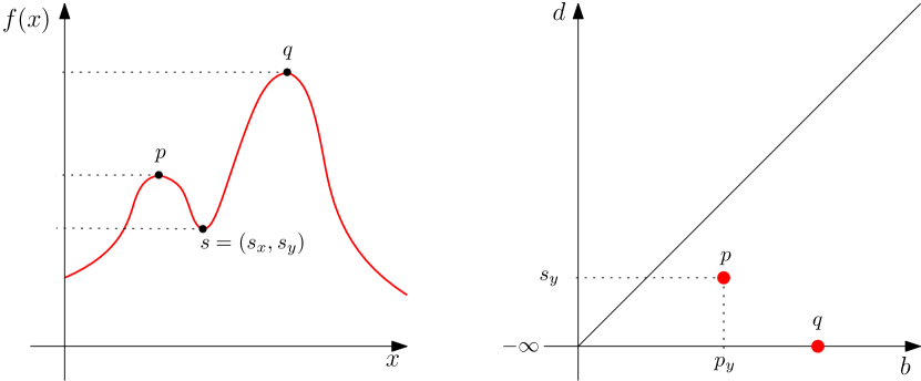
Figure 1: (a) A function $f\colon\mathbb{R}\to\mathbb{R}$ with local peaks $p$ and $q$. (b) Dgm($X,f$) for the function on the left.

A standard measure of similarity between persistence diagrams is the bottleneck distance [EH10, COGDS16].

Definition 2.5.

Let $\mathrm{Dgm}_{1}$ and $\mathrm{Dgm}_{2}$ be two persistence diagrams that have finitely many points off the diagonal. Let $\pi$ denote the set of bijections $\nu\colon\mathrm{Dgm}_{1}\to\mathrm{Dgm}_{2}$. Given points $x=(x_{1},x_{2})$ and $y=(y_{1},y_{2})$ in $\overline{\mathbb{R}}^{2}$, let $\|x-y\|_{\infty}=\max\{|x_{1}-y_{1}|,|x_{2}-y_{2}|\}$ denote their $L^{\infty}$-distance, where we set $(+\infty)-(+\infty)=(-\infty)-(-\infty)=0$. Then, the bottleneck distance between $\mathrm{Dgm}_{1}$ and $\mathrm{Dgm}_{2}$ is defined as

$$W_{\infty}(\mathrm{Dgm}_{1},\mathrm{Dgm}_{2})=\displaystyle\inf_{\nu\in\pi}\sup_{x\in\mathrm{Dgm}_{1}}\|x-\nu(x)\|_{\infty}.$$

Note that a bijection $\nu\colon\mathrm{Dgm}_{1}\to\mathrm{Dgm}_{2}$ is allowed to match an off-diagonal point of $\mathrm{Dgm}_{1}$ to the diagonal of $\mathrm{Dgm}_{2}$, and vice versa.

Persistence diagrams are stable with respect to small perturbations [CSEH07], i.e. for ${f,g\colon X\to\mathbb{R}}$

$$W_{\infty}(\textrm{Dgm}(X,f),\textrm{Dgm}(X,g))\leq\|f-g\|_{\infty}$$

under certain assumptions on $(X,f)$ and $(X,g)$. This holds, for example, if $f,g$ are Morse functions on compact manifolds, piecewise linear functions on simplicial complexes, etc. There are versions of the stability result that hold more generally, for example [CdSO14, CdSMS16, CCSG⁺09].

Example 2.6.

Consider a function $f$ defined on a compact subset of $\mathbb{R}$ and a piecewise linear approximation of $f$, $g$ (Figure 2). Since the functions are close to each other with respect to the $L^{\infty}$ distance, the stability theorem guarantees that the corresponding persistence diagrams are close with respect to the bottleneck distance. Indeed, the number of prominent peaks is the same in both cases.

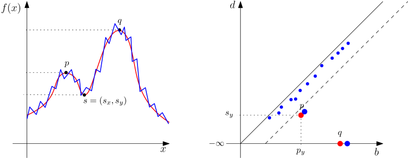
Figure 2: (a) A function $f\colon K\subset\mathbb{R}\to\mathbb{R}$ and an approximation of $f$, $g$. (b) Dgm($X,f$) consists of red dots, while Dgm($X,g$) consists of the blue dots.

2.2 ToMATo: a Persistence-Based Clustering Algorithm

We now briefly recall how the ToMATo clustering algorithm works. Given a point cloud $X$ ToMATo relies on the assumption that the points of $X$ were sampled according to some unknown density function $f$. In a nutshell, ToMATo infers information about the local maxima of $f$ by applying the above procedure to an estimate of $f$. ToMATo takes as input:

• A neighborhood graph $G$ on the points of $X$. Chazal et al. mostly use the $\delta$-Rips graph and the $k$-nearest neighbor graph.

• A density estimator $\hat{f}$. Each vertex $v$ of $G$ is assigned a non-negative value $\hat{f}(v)$ that corresponds to the estimated density at $v$. Chazal et al. propose two possible density estimators: the truncated Gaussian kernel density estimator and the distance-to-measure density, originally introduced in [BCCS⁺11].

• A merging parameter $\tau\geq 0$. This is a threshold that the prominence of a local maximum of the estimated density $\hat{f}$ must clear for that local maximum to be deemed a feature.

Given the inputs above, ToMATo proceeds as follows.

1. Estimate the underlying density function $\hat{f}$ at the points of $X$.

2. Apply a hill-climbing algorithm on $G$. Construct the neighborhood graph $G$ on the points of $X$, and construct a directed subgraph $\Gamma$ of $G$ as follows: at each vertex $v$ of $G$, place a directed edge from $v$ to its neighbor with highest value of $\hat{f}$, provided that that value is higher than $\hat{f}(v)$. If all neighbors of $v$ have lower values, $v$ is a peak of $\hat{f}$. This yields a collection of directed edges that form a spanning forest of the graph $G$, consisting of one tree for each local maximum of $\hat{f}$. In particular, these trees yield a partition of the elements of $X$ into pairwise disjoint sets that serves as a candidate clustering on $X$.

3. Construct the persistence diagram. Construct the persistence diagram $\mathrm{Dgm}(G,\hat{f})$ associated to the superlevelset filtration of $\hat{f}\colon G\to\mathbb{R}$.

4. Merge non-significant clusters. Iteratively merge every cluster of prominence less than $\tau$ of the candidate clustering found in Step 2 into its parent cluster, i.e., into the cluster corresponding to the local maximum that it gets merged into in the superlevelset filtration of $\hat{f}\colon G\to\mathbb{R}$. ToMATo outputs the resulting clustering of points of $X$, in which every cluster has prominence at least $\tau$ by construction.

The reason why we can expect the persistence diagram of the approximated density to be “close” to the original one stems from the stability of persistence diagrams under the bottleneck distance, as explained in Section 2.1 and illustrated in Figure 2.

In practice, the user must run ToMATo twice. First, ToMATo is run with $\tau=+\infty$, which is equivalent to computing the birth and death time of each local maximum of $\hat{f}$ and hence the persistence diagram $\mathrm{Dgm}(G,\hat{f})$. From the diagram $\mathrm{Dgm}(G,\hat{f})$ the user then determines a merging parameter $\tau$ by visually identifying a large gap in $\mathrm{Dgm}(G,\hat{f})$ separating, say, $C$ points corresponding to highly prominent peaks from the rest of the points. Then, ToMATo is run a second time with $\tau$ set to that value, which results in the final clustering of $X$ into $C$ clusters.

2.3 The Bottleneck Bootstrap

We now review the second ingredient of our clustering scheme, a procedure known as the bottleneck bootstrap. Introduced in [CFL⁺17, Section 6], it is used to separate significant features in persistence diagrams from non-significant ones. While it may be used in more general settings, we will restrict ourselves to the scenario of Section 2.2

Suppose that $X$ is a sample consisting of $n$ data points, drawn according to some unknown probability density function $f\colon K\to[0,1]$, $K\subset\mathbb{R}^{n}$, and let $\mathcal{D}:=\mathrm{Dgm}(K,f)$ denote the corresponding (unknown) persistence diagram (we assume the density $f$ and all of its estimates to be normalized here for ease of exposition). We estimate $f$ and the connectivity of $K$ with a density estimator and a neighborhood graph, respectively (as explained in Section 2.2). This allows us to compute $\widehat{\mathcal{D}}:=\mathrm{Dgm}(X,\hat{f})$, where $\hat{f}$ is the estimate of $f$). The diagram $\widehat{\mathcal{D}}$ serves as an estimate for $\mathcal{D}$.

Given a confidence level $\alpha\in(0,1)$ and a number $B\in\mathbb{Z}_{\geq 1}$ of bootstrap iterations, the bottleneck bootstrap gives an estimate $\widehat{q}_{\alpha}$ of $q_{\alpha}$, which is defined by

$$\mathbb{P}(\sqrt{n}W_{\infty}(\mathcal{D},\widehat{\mathcal{D}})\leq q_{\alpha})=1-\alpha.$$ (1)

In order to produce $\widehat{q}_{\alpha}$, we first approximate $f$ with the empirical measure $P_{n}$ on $X$ that assigns the probability mass of $1/n$ to each data point (note that this generally does not coincide with $\hat{f}$). This allows us to estimate the distribution

$$F(z):=\mathbb{P}(\sqrt{n}W_{\infty}(\mathcal{D},\widehat{\mathcal{D}})\leq z)$$

with the distribution

$$\widehat{F}(z):=\mathbb{P}(\sqrt{n}W_{\infty}(\widehat{\mathcal{D}}^{*},\widehat{\mathcal{D}})\leq z),$$

where $\widehat{\mathcal{D}}^{*}:=\mathrm{Dgm}(X^{*},\hat{f}^{*})$ is the persistence diagram corresponding to a sample $X^{*}$ of size $n$ drawn from $P_{n}$, and the density $\hat{f}^{*}$ and the connectivity of $X^{*}$ are estimated using the same estimators as before. Note that $X^{*}$ may be thought of as a sample drawn from $X$ with replacement. The distribution $\widehat{F}$ itself is approximated by Monte Carlo as follows. We draw $B$ samples $X_{1}^{*},\dots,X_{B}^{*}$ of size $n$ from $P_{n}$, and for each of these $B$ samples, we compute the persistence diagram $\widehat{\mathcal{D}}_{i}^{*}:=\mathrm{Dgm}(X_{i}^{*},\hat{f}_{i}^{*})$ and the quantity $T_{i}^{*}:=\sqrt{n}W_{\infty}(\widehat{\mathcal{D}}_{i}^{*},\widehat{\mathcal{D}})$, $i=1,\dots,B$. Finally, we use the function

$$\widetilde{F}(z):=\frac{1}{B}\sum_{i=1}^{B}\mathbf{1}_{[0,z]}(T_{i}^{*})$$

as an approximation of $\widehat{F}$, and hence of $F$. Using this, we set

$$\widehat{q}_{\alpha}:=\inf\{z\mid\widetilde{F}(z)\geq 1-\alpha\}$$

to be our estimate of $q_{\alpha}$. This estimate is asymptotically consistent if $\sup_{z}|\widetilde{F}(z)-F(z)|\xrightarrow{f}0$. If that is the case, it follows from Equation 1 that (asymptotically) the true, unknown persistence diagram $\mathcal{D}$ is at bottleneck distance of at most $\widehat{q}_{\alpha}/\sqrt{n}$ from $\widehat{\mathcal{D}}$. Hence, points of $\widehat{\mathcal{D}}$ that are at $L^{\infty}$-distance at most $\widehat{q}_{\alpha}/\sqrt{n}$ from the diagonal could be matched to the diagonal under the bottleneck distance, and thus a point of $\widehat{\mathcal{D}}$ is declared to be a significant feature iff it is at $L^{\infty}$-distance of at least $\widehat{q}_{\alpha}/\sqrt{n}$ to the diagonal, i.e., iff its prominence is at least $2\cdot\widehat{q}_{\alpha}/\sqrt{n}$.

2.4 Clustering

Clustering is a fundamental technique in unsupervised learning and thus there is a vast body of literature both on the theoretical foundation as well as on various algorithms and applications of clustering [And73, DHS00]. Very roughly, most clustering algorithms fall into one of four categories: centroid-based algorithms, model-based algorithms, hierarchical clustering algorithms, and density-based algorithms.

The most famous algorithm in the first category is $k$-means, see [Boc07] for a historic overview. The $k$-means algorithm and many other centroid-based algorithms take the number of clusters as an input, rendering them irrelevant for many applications such as Mapper. We thus do not compare our new algorithm against $k$-means and similar algorithms. Similarly, we omit comparisons with model-based algorithms since they assume that the data follows some distribution, which is an assumption we do not make.

Hierarchical clustering algorithms start by considering each data point as its own cluster and iteratively join the two currently closest clusters into a single cluster, stopping either when a certain number of clusters is reached or when any two clusters are far enough apart. As such, they use one of the following two as a hyperparameter: the number of clusters or a distance threshold. Depending on how the distance between clusters is defined, one obtains different hierarchical clustering algorithms. We compare our algorithms against several such algorithms. In single linkage clustering the distance between two clusters $A$ and $B$ is defined as $\min_{a\in A,b\in B}d(a,b)$. Replacing the $\min$ by $\max$, we get the distance function for complete linkage clustering. For average linkage clustering, the distance between two clusters $A$ and $B$ is the average distance between the points, that is, $\frac{1}{|A|\cdot|B|}\sum_{a\in A}\sum_{b\in B}d(a,b)$. Finally, in Ward linkage clustering, the distance between two clusters $A$ and $B$ is defined in terms of their centroids $\mu_{A}$ and $\mu_{B}$ by $\frac{|A|\cdot|B|}{|A\cup B|}\lVert\mu_{a}-\mu_{b}\rVert^{2}$. For surveys on different hierarchical clustering algorithms and a comparison between them we refer to [MT13, SB⁺19].

Among the most widely used density-based clustering algorithms are DBSCAN [EKSX96] and its adaptation HDBSCAN [CMS13]. DBSCAN has two hyperparameters, a natural number $\mathrm{minPts}$ and a distance threshold $\varepsilon$. Any data point that contains at least $\mathrm{minPts}$ in its ball of radius $\varepsilon$ is called a core point. DBSCAN then assigns two core points to the same cluster whenever the distance between them is at most $\varepsilon$ and also adds all points in their $\varepsilon$-balls to this cluster. Any (non-core points) that are not assigned to any cluster are labelled as noise. HDBSCAN is an extension of DBSCAN that, roughly speaking, performs the same procedure for a range of values for $\varepsilon$ and computes for each potential cluster a stability value, selecting as final clusters those whose stability is greater than the sum of stability values of its subclusters. We include both DBSCAN and HDBSCAN in our comparison.

A clustering method is parameter-free if it does not depend on a good choice of hyperparameters. Several such methods have been introduced in the literature, often for specialized tasks. There is also some recent work on parameter-free clustering methods that are designed for general settings. Among those we mention some for which there are publicly available implementations, which allows us to compare our new algorithm against them. These are FINCH [SSS19] and the persistence-based clustering algorithm [CSTL21] implemented in the Topology ToolKit [CSTL21]. In a nutshell, FINCH proceeds as follows. The algorithm defines a graph on the data points, connecting two points $a$ and $b$ whenever $a$ is the closest neighbor to $a$ or vice versa, or if the two of them have the same closest neighbor. The initial clusters are then the connected components of this graph. In a second step, some of the clusters get merged in a similar fashion as in hierarchical clustering algorithms until only a previously estimated number of clusters is left. The persistence-based clustering algorithm from from the Topology ToolKit, on the other hand, is similar to AuToMATo insofar as that it produces a persistence diagram of an estimated density function, and then determines how many points in that diagram correspond to “significant" topological features, thus automating the selection of numbers of clusters in ToMATo. Unlike AuToMATo, however, that algorithm does so by making the assumption that the lifetimes of non-significant features roughly follow some exponential, and then declares a point of the estimated persistence diagram to be a feature if it deviates from the estimated exponential curve.

One way of evaluating the clustering performance of an algorithm is to compare the clusterings found by the algorithm to a ground truth clustering. There are many metrics that may be used to that end: for example, set-matching-based, information theoretic, and pair-counting-based metrics [RF16, VEB10]. Set-matching-based metrics rely on finding matches between clusters in the two clusterings. A notable representative of this is the classification error rate, which is often employed in supervised learning. Information-theoretic-based metrics are built upon fundamental concepts from information theory and include the mutual information (MI) score [VEB10], the normalized mutual information score (NMI) etc. Pair-counting-based measures are built upon counting pairs of items on which two clusterings agree or do not agree. Examples of measures that fall into this category are the Rand index [Ran71] and the Fowlkes-Mallows score [FM83], which we use in this paper.

The Fowlkes-Mallows score was originally defined for hierarchical clusterings only, however, it may be defined for general clusterings as follows. Given a clustering $C$ found by an algorithm and a ground truth clustering $G$, one defines the Fowlkes-Mallows score as

$$\mathrm{FMS}:=\sqrt{\frac{\mathrm{TP}}{\mathrm{TP}+\mathrm{FP}}}\cdot\sqrt{\frac{\mathrm{TP}}{\mathrm{TP}+\mathrm{FN}}},$$

where

• $\mathrm{TP}$ is the number of pair of data points which are in the same cluster in $C$ and in $G$;

• $\mathrm{FP}$ is the number of pair of data points which are in the same cluster in $G$ but not in $C$; and

• $\mathrm{FN}$ is the number of data points which are not in the same cluster in $G$ but are in the same cluster in $C$.

In other words, the Fowlkes-Mallows score is defined as the geometric mean of precision and recall of a classifier whose relevant elements are pairs of points that belong to the same cluster in both $C$ and $G$. As such, this score may attain any value between 0 and 1, and these extremal values correspond to the worst and best possible clustering, respectively.

3 Methodology and implementation of AuToMATo

3.1 Methodology of AuToMATo

AuToMATo builds upon the ToMATo clustering scheme introduced in [CGOS13] and implemented in [Gli23]. AuToMATo automates the step of visual inspection of the persistence diagram by means of the bottleneck bootstrap, thus promoting ToMATo to a clustering scheme that does not rely on human input.

More precisely, given a point cloud $X$ to perform the clustering on, AuToMATo takes as input

• an instance of ToMATo with fixed neighborhood graph and density function estimators;

• a confidence level $\alpha\in(0,1)$; and

• a number of bootstrap iterations $B\in\mathbb{Z}_{\geq 1}$.

Remark 3.1.

We point out that our implementation of AuToMATo comes with default values for each of the objects. Each of these values can, of course, be adjusted by the user. For details on these default values, see Section 3.2.

In the present context the bottleneck bootstrap proceeds as follows. AuToMATo generates $B$ bootstrap subsamples $X_{1}^{*},\dots,X_{B}^{*}$ of $X$, each of the same cardinality as $X$. Then, the underlying ToMATo instance with $\tau=+\infty$ and its neighborhood graph and density function estimators is used to compute the persistence diagram for $X$ and each of $X_{1}^{*},\dots,X_{B}^{*}$, yielding persistence diagrams $\widehat{\mathcal{D}}$ and $\widehat{\mathcal{D}}_{1}^{*},\dots,\widehat{\mathcal{D}}_{B}^{*}$, respectively. Using the bootstrapped diagrams $\widehat{\mathcal{D}}_{1}^{*},\dots,\widehat{\mathcal{D}}_{B}^{*}$, a bottleneck bootstrap is performed on $\widehat{\mathcal{D}}$. This yields a value $\widehat{q}_{\alpha}$ that (asymptotically as $n\to\infty$) satisfies

$$\mathbb{P}(\sqrt{n}W_{\infty}(\mathcal{D},\widehat{\mathcal{D}})\leq\widehat{q}_{\alpha})=1-\alpha,$$

where $\mathcal{D}$ denotes the persistence diagram of the true, unknown density function from which $X$ was sampled. Thus, points of $\widehat{\mathcal{D}}$ of prominence at least $2\cdot\widehat{q}_{\alpha}/\sqrt{n}$ are declared to be significant features of $\widehat{\mathcal{D}}$, and AuToMATo outputs its underlying ToMATo instance with prominence threshold set to $\tau=2\cdot\widehat{q}_{\alpha}/\sqrt{n}$.

When computing the values $\sqrt{n}W_{\infty}(\widehat{\mathcal{D}}_{i}^{*},\widehat{\mathcal{D}})$, $i=1,\dots,B$, in the bottleneck bootstrap, we only consider points in $\widehat{\mathcal{D}}_{i}^{*}$ and $\widehat{\mathcal{D}}$ with finite lifetimes. The reason for this choice is that we consider peaks with infinite lifetime to be significant a priori. Moreover, some of the bootstrapped diagrams among the $\widehat{\mathcal{D}}_{1}^{*},\dots,\widehat{\mathcal{D}}_{B}^{*}$ have a different number of points with infinite lifetime than the reference diagram $\widehat{\mathcal{D}}$. In these cases, the bottleneck distance of the bootstrapped diagram to the reference diagram is infinite, which heavily distorts the distribution $\widetilde{F}(z)$. This choice is justified by experiments.

3.2 Implementation of AuToMATo

We implemented AuToMATo in Python, and all of the code with documentation is available on GitHub. For a description of AuToMATo in pseudocode, see Algorithm 1. The algorithm has a worst-case complexity of $O(B(nd+n\log(n)+N^{1.5}\log N))$, where $d$ is the dimensionality of the data and $N$ is the maximal number of off-diagonal points across all relevant persistence diagram (which is generally much smaller than $n$); see Appendix A.1 for details. Note that the factor of $B$ can be significantly decreased through parallelization.

Input: point cloud $X$ of $n$ data points; instance $\mathrm{tom}_{\tau}$ of ToMATo with neighborhood graph and density function estimators, and prominence threshold $\tau$; confidence level $\alpha\in(0,1)$; number of bootstrap iterations $B\in\mathbb{Z}_{\geq 1}$.

$\mathcal{D}\leftarrow\mathrm{Dgm}(\mathrm{tom}_{\infty}(X))$ ;

  // compute persistence diagram of point cloud

for $i=1$ to $B$ do

       Let $X_{i}^{*}$ be a subsample of $X$ of size $n$, sampled with replacement;

       $\mathcal{D}_{i}^{*}\leftarrow\mathrm{Dgm}(\mathrm{tom}_{\infty}(X_{i}^{*}))$ ;

        // compute persistence diagram of subsample

       $d_{i}\leftarrow\sqrt{n}W_{\infty}^{\mathrm{fin}}(\mathcal{D}_{i}^{*},\mathcal{D})$ ;

        // compute bottleneck distance between finite points

      

end for

Sort and reindex $\{\mathcal{D}_{1}^{*},\dots,\mathcal{D}_{B}^{*}\}$ such that $d_{1}\leq\cdots\leq d_{B}$;

$k\leftarrow\lceil(1-\alpha)\cdot B\rceil$;

$\widehat{q}_{\alpha}\leftarrow d_{k}$;

$\tau\leftarrow 2\cdot\widehat{q}_{\alpha}/\sqrt{n}$;

Output: $\mathrm{tom}_{\tau}(X)$ ;

  // copy of initial ToMATo instance with prominence threshold set to $\tau$

Algorithm 1 AuToMATo

While the input parameters may be adjusted by the user, the implementation provides default values whose choices we discuss presently.

Choice of ToMATo parameters:

Our implementation of AuToMATo is such that the user can directly pass parameters to the underlying ToMATo instance. If no such arguments are provided AuToMATo uses the default choices for those parameters, as determined by the implementation of ToMATo given in [Gli23]. In particular, AuToMATo uses the $k$-nearest neighbor graph and the (logarithm of the) distance-to-measure density estimators by default, each with $k=10$. Of course, the persistence diagrams produced by ToMATo, and hence the output of AuToMATo, depend on this choice. This can lead to suboptimal clustering performance of AuToMATo; see Section 6.

Choice of $\alpha$ and $B$:

By default, AuToMATo performs the bootstrap on $B=1000$ subsamples of the input point cloud, and sets the confidence level to $\alpha=0.35$. The choice of this latter parameter means that AuToMATo determines merely a 65% confidence region for the persistence diagram produced by the underlying ToMATo instance. While in bootstrapping the confidence level is often set to e.g. $\alpha=0.05$, the seemingly strange choice of $\alpha=0.35$ in the setting of AuToMATo is justified by experiments. The value of 65% seems to be low enough to offset some of the negative influence of using possibly non-optimized neighborhood graph and density estimators discussed in Section 6, while at the same time being high enough to yield good results when these estimators are chosen suitably. We point out that the value $\alpha=0.35$ (as well as the value $B=1000$) was decided on after running an early implementation of AuToMATo on just a few synthetic data sets. In particular, the choice was made before conducting the experiments in Section 4. AuToMATo is implemented in such a way that the parameter $\alpha$ can be adjusted after fitting and the clustering is automatically updated.

Our Python package for AuToMATo consists of two separate modules; one for AuToMATo itself, and one for the bottleneck bootstrap. Both are compatible with the scikit-learn architecture, and the latter may also be used as a stand-alone module for other scenarios. In addition to the functionality inherited from the scikit-learn API, the implementation of AuToMATo comes with options of

• adjusting the parameter $\alpha$ of a fitted instance of AuToMATo which automatically updates the resulting clustering without repeating the (computationally expensive) bootstrapping;

• plotting the persistence diagram and the prominence threshold found in the bootstrapping;

• setting a seed in order to make the creation of the bootstrap subsamples in AuToMATo deterministic, thus allowing for reproducible results; and

• parallelizing the bottleneck bootstrap for speed improvements.

Finally, our implementation of AuToMATo contains a parameter that allows the algorithm to label points as outliers. In a nutshell, a point is classified as an outlier if it is not among the nearest neighbors of more than a specified percentage of its own nearest neighbors. This feature, however, is currently experimental (and is thus turned off by default).

4 Experiments

4.1 Choice of clustering algorithms for comparison

We chose to compare AuToMATo with its default parameters against

• DBSCAN and its extension HDBSCAN;

• hierarchical clustering with Ward, single, complete and average linkage;

• the FINCH clustering algorithm [SSS19]; and

• a clustering algorithm building on ToMATo stemming from the Topology ToolKit (TTK) suite [TFL⁺18]; in the following, we will refer to this as the TTK-algorithm.

For DBSCAN, HDBSCAN and the hierarchical clustering algorithms mentioned above, we worked with their implementations in scikit-learn. For the FINCH clustering algorithm, we worked with the version available on GitHub. Indeed, we subclassed that version in order to make it compatible with the scikit-learn API. Similarly, we created a scikit-learn compatible version of the TTK-algorithm by combining code from TTK with the description of the algorithm given in [CSTL21, Section 5.2]. While we included DBSCAN and HDBSCAN among the clustering algorithms to compare AuToMATo against because they are standard choices, we chose to include the hierarchical clustering algorithms because they are readily available through scikit-learn. Finally, we chose to include FINCH and the TTK-algorithm because, like AuToMATo, they are parameter-free methods and are thus especially interesting to compare AuToMATo against.

4.2 Choice of data sets

The data sets on which we ran AuToMATo and the above clustering algorithms stem from the Clustering Benchmarks suite. We chose this collection as it comes with a large variety of different data sets, all of which are labeled by one or more ground truths, allowing for a fair and extensive comparison. The collection contains five recommended batteries of data sets from which we selected those (data set, ground truth)-pairs that we deemed reasonable for a general purpose parameter-free clustering algorithm. For instance, we chose not to include the data set named olympic that is part of the wut-battery, but we did include the data set named windows from the same battery. Both of these are illustrated in Figure 3.

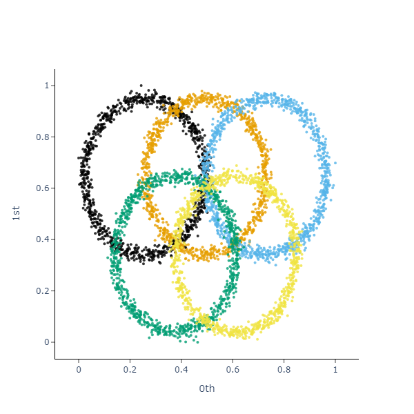
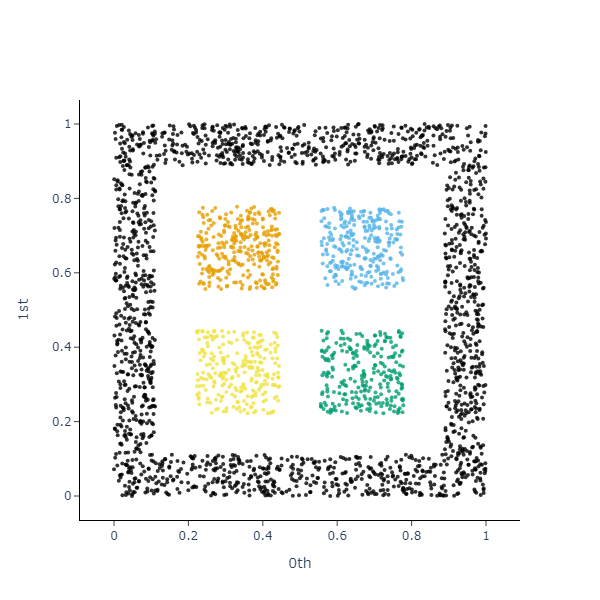
Figure 3: The olympic and windows data sets from the wut-battery.

We chose the wut-battery dataset because AuToMATo is a clustering algorithm that determines clusters depending on connectivity, and topologically speaking, there is only one connected component in the wut-battery dataset.

Finally, we excluded all instances where the ground truth contains data points that are labeled as outliers, as outliers creation is currently an experimental feature in AuToMATo.

4.3 Methodology of the experiments

We min-max scaled each data set, fitted the clustering algorithms to them, and recorded the clustering performance of each result by computing the Fowlkes-Mallows score (see Section 2.4) of the clustering obtained and the respective ground truth. We chose not to use the Rand index or other scores mentioned in Section 2.4 because those have been shown to exhibit biased behaviour depending on whether the clusters in the ground truth are mostly of similar sizes or not, see e.g. [RVBV16]. To the best of our knowledge, the Fowlkes-Mallows score does not suffer from such drawbacks.

Since AuToMATo contains a randomized component (namely, the creation of bootstrap samples), we chose to run it ten times on each dataset and report its average performance. Moreover, we set the hyperparameters of the HDBSCAN, FINCH and the TTK-algorithm to their default values (as per their respective implementations). In contrast to this, we let the distance threshold parameter for the DBSCAN and the hierarchical clustering algorithms vary from 0.05 to 1.00 in increments of 0.05, with the goal of comparing AuToMATo against the best and worst performing version of these clustering algorithms.

While we restricted ourselves to instances where the ground truth does not contain any points labeled as outliers, some of the clustering algorithms in our list (DBSCAN and HDBSCAN) label some data points as outliers. In order to prevent these algorithms from getting systematically low Fowlkes-Mallows scores because of these outliers, we removed all the points labeled as outliers by these algorithms, and only computed the Fowlkes-Mallows score on the remaining points, both for these clustering algorithms and for AuToMATo. This of course gives an advantage to DBSCAN and HDBSCAN over AuToMATo. Finally, since AuToMATo is not entirely deterministic, we ran AuToMATo on each dataset ten times, and recorded the mean of the Fowlkes-Mallows score.

In order to allow reproducibility, we chose a fixed seed for all our experiments, which can be found in our code on GitHub. We ran our experiments on a laptop with a 12th Gen Intel Core i7-1260P processor running at 2.10GHz.

4.4 Results and interpretation

Table LABEL:table:summary_of_results shows the average Fowlkes-Mallows score of each algorithm across all benchmarking data sets. Moreover, in the case of AuToMATo, this table reports the mean and the standard deviation of the Fowlkes-Mallows score across the ten runs. For those benchmarking data sets that come with more than one ground truth, we included only the best score of the respective algorithm. Similarly, we included only the best performing parameter selection for those algorithms that we ran with varying distance thresholds (which, of course, skews the comparison in favor of those algorithms). As Table LABEL:table:summary_of_results shows, AuToMATo outperforms each clustering algorithm on average across all data sets, thus showing that it is indeed a versatile and powerful out-of-the-box clustering algorithm. In particular, AuToMATo outperforms the TTK-algorithm, which also build on ToMATo.

Table 1: Average clustering performance of AuToMATo vs. reference clustering algorithms

Algorithm	Fowlkes-Mallows score
AuToMATo	0.8620±0.0202
DBSCAN	0.8482
Average linkage	0.8349
HDBSCAN	0.8270
Single linkage	0.8191
TTK clustering algorithm	0.8189
Complete linkage	0.7651
Ward linkage	0.5916
FINCH	0.4983

Table 1: Average clustering performance of AuToMATo vs. reference clustering algorithms

Of course, we do not claim that AuToMATo outperforms each of the algorithms above on every single data set. Indeed, seeing that we ran DBSCAN with a wide range of choices for the distance threshold parameter, it is to be expected that the best choice of parameter should often outperform AuToMATo. However, on most data sets where this is the case, the results from AuToMATo are still competitive. In fact, there are a significant number of instances where AuToMATo outperforms DBSCAN for all parameter selections, in some cases by a lot. This is illustrated in Figure 4, where we show the Fowlkes-Mallows score of AuToMATo and each of the best and worst performing parameter choice of DBSCAN across all datasets.

Figure 4: Comparison of AuToMATo and DBSCAN.

The scores of our experiments are reported in Tables LABEL:table:aut_vs_dbscan through LABEL:table:aut_vs_ttk in Appendix A.2, and each of these tables is accompanied by a figure similar to Figure 4.

5 Applications of AuToMATo in Combination with Mapper

The goal of Mapper [SMC⁺07] is to approximate the Reeb graph of a manifold $M$ based on a sample from $M$. The input is a point cloud $P$ with a filter function $P\rightarrow\mathbb{R}$, a collection of overlapping intervals $\mathcal{U}=\{U_{1},\ldots,U_{n}\}$ covering $\mathbb{R}$ and a clustering algorithm. For each $U_{i}\in\mathcal{U}$, Mapper runs the clustering algorithm on the data points in the preimage $f^{-1}(U_{i})$, creating a vertex for each cluster. Two vertices are then connected by an edge if the corresponding clusters (in different preimages) have some data points in common, yielding a graph that represents the shape of the data set.

We ran the Mapper implementation of giotto-tda [TLT⁺20] on a synthetic two-dimensional data set consisting of noisy samples from two concentric circles (see Figure 5(a)) with projection onto the $x$-axis as the filter function. We ran Mapper on the same interval cover with three different choices of clustering algorithms: AuToMATo, DBSCAN, and HDBSCAN (the latter two with their respective default parameters). As can be seen in Figure 5(b), using DBSCAN, we get many unwanted edges in the graph. HDBSCAN performs better, giving two cycles with some extra loops. The output of Mapper with AuToMATo is exactly the Reeb graph of two circles.

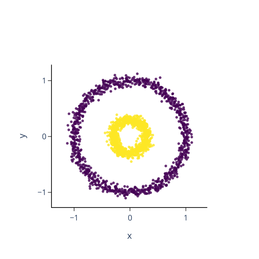
(a)

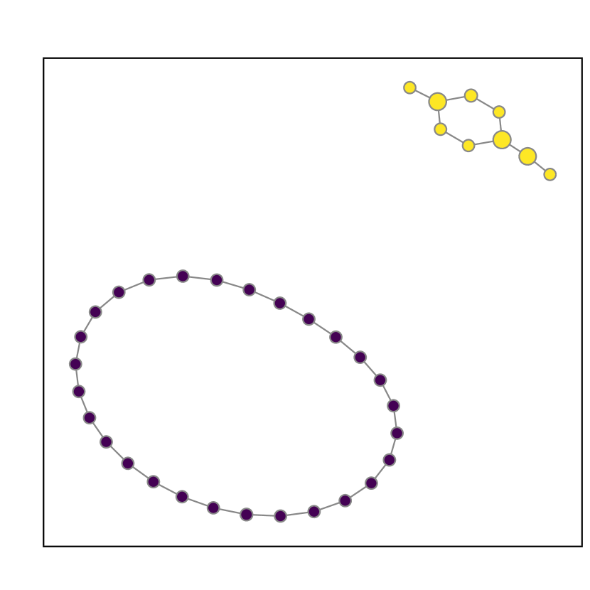
(b)

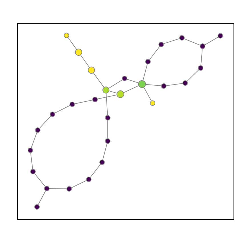
(c)

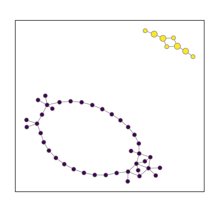
(d)

Figure 5: (a) input data set; result of Mapper with (b) AuToMATo; (c) DBSCAN; (d) HDBSCAN

We further tested the combination of Mapper with AuToMATo on one of the standard applications of Mapper: the Miller-Reaven diabetes data set, where Mapper can be used detect two strains of diabetes that correspond to “flares” in the data set (see [SMC⁺07, Section 5.1] for details). As can be seen in Figure 6, AuToMATo performs well in this task; the graphs show a central core of vertices corresponding to healthy patients, and two flares corresponding to the two strains of diabetes. We were not able to reproduce this using DBSCAN or HDBSCAN; Figure 6 shows the output of Mapper with these algorithms with their respective default parameters.

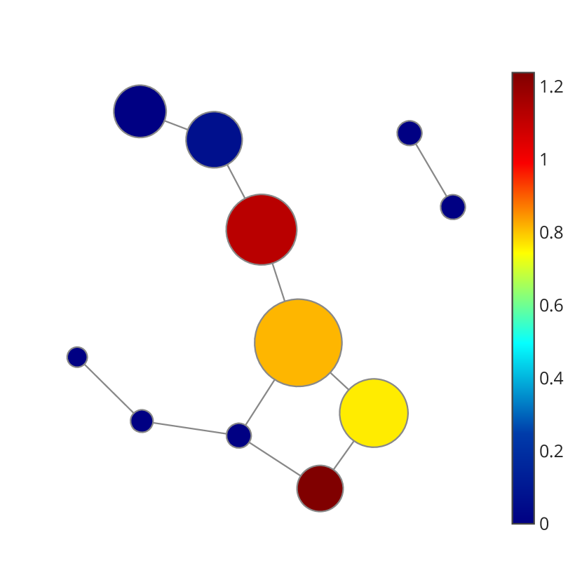
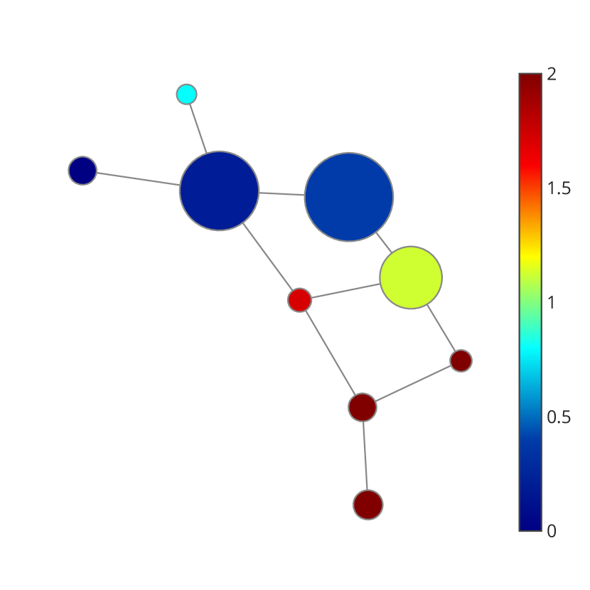
Figure 6: Mapper applied to the diabetes data set with AuToMATo (left); DBSCAN (center); HDBSCAN (right). Labels 0, 1 and 2 stand for “no ”, “chemical” and “overt diabetes”.

6 Discussion

We briefly outline some limitations of AuToMATo. As mentioned in Remark 3.1, AuToMATo comes with a choice of default values for its parameters that make it perform well in experiments. In particular, AuToMATo resorts to the default values as implemented in ToMATo for the choice of neighborhood graph and density estimators. In ToMATo, the options for the neighborhood graph estimators are the $\delta$-Rips graph and the $k$-nearest neighbor graph, relying on parameters $\delta>0$ and $k\geq 1$, respectively; the options for the density estimators are the kernel density estimator and the distance-to-measure density estimator, which in turn rely parameters $h>0$ and $m\in(0,1)$, respectively (see the footnotes in Section 2.2 for their definitions). While for most data sets that we ran our experiments on these default estimators yielded good results, there are cases where adjusting them before running AuToMATo improves the clustering performance. Nevertheless, since finding a priori optimal parameters for the neighborhood graph and density estimators for a given data set is largely an open problem, we chose to stick to the default values for these estimators. Indeed, there are heuristics for the selection of the bandwidth in kernel density estimation (see [CSTL21, Section 4.1]) and the smoothing parameter in distance-to-measure density estimation (see [CFL⁺17, Section 7.1]), but these methods either lack theoretical justification, or would require running AuToMATo multiple times on the same data set with different parameters and selecting the best ones a posteriori, effectively rendering AuToMATo a non-parameter-free clustering algorithm.

Optimizing the choice of the neighborhood graph and density estimators is an aspect of AuToMATo that we plan to pursue in future work. Moreover, we plan to improve the currently experimental feature for outlier creation in AuToMATo discussed at the end of Section 3.2. Finally, it is natural to ask whether the results from [CMO18] on optimal parameter selection in the Mapper algorithm can be adapted to the scenario where Mapper uses AuToMATo as its clustering algorithm.

Appendix A Appendix

A.1 Complexity analysis of Algorithm 1

Recall from [CGOS13, Section 2] that, if an estimated density and a neighborhood graph are provided, ToMATo has a worst-case time complexity in $O(n\log(n)+m\alpha(n))$, where $n$ and $m$ are the number of vertices and edges of the neighborhood graph, respectively, and $\alpha$ denotes the inverse Ackermann function (note that $n$ equals the number of data points). By default, ToMATo (and hence AuToMATo) works with the $k$-nearest neighbor graph and distance-to-measure density estimators, where the latter relies itself on the $k$-nearest neighbor graph (each with $k=10$). Taking into account the known complexity bound $O(nd)$ for the creation of the $k$-nearest neighbor graph (where $d$ is the dimensionality of the data), and using the fact that $m\in O(n)$ for this graph, this leads to a worst-case time complexity in $O(nd+n\log(n))$ for a single run of ToMATo. Creating the bootstrap samples $X_{i}^{*}$, $i=1,\dots,B$, has complexity in $O(Bn)$; computing the values $\sqrt{n}W_{\infty}^{\mathrm{fin}}(\mathcal{D}_{i}^{*},\mathcal{D})$, $i=1,\dots,B$, has worst-case complexity $O(BN^{1.5}\log(N))$ (see e.g. [EIK01]; here $N$ denotes the maximal number of off-diagonal points across all relevant persistence diagram), and sorting them has worst case complexity in $O(B\log(B))$. Combined, this leads to a worst-case complexity for AuToMATo in $O(B(nd+n\log(n)+N^{1.5}\log(N))+B\log(B))$. Using that $B$ is a constant, we obtain the runtime claimed in the main body.

A.2 Benchmarking results

In this subsection we report the Fowlkes-Mallows scores coming from comparing AuToMATo to the other clustering algorithms, as explained in Section 4. For those benchmarking data sets that come with more than one ground truth, we report the scores for each of those, and different ground truths are indicated by the last digit in the data set name. Moreover, each table is sorted according to increasing difference in clustering performance of AuToMATo and the respective clustering algorithm that AuToMATo is being compared against. As is customary, we indicate the score stemming from the best performing clustering algorithm in bold.

Table 2: Fowlkes-Mallows scores of AuToMATo vs. DBSCAN

Dataset	automato_mean	dbscan_max	dbscan_min
sipu_r15_2	0.4867±0.0000	1.0000	0.5607
wut_trajectories_0	0.5038±0.0107	1.0000	0.4999
wut_x3_0	0.5153±0.0000	0.9398	0.5149
wut_x2_0	0.5846±0.0000	0.9483	0.5779
sipu_r15_1	0.5436±0.0000	0.8954	0.5021
fcps_tetra_0	0.6261±0.0000	0.9403	0.0000
sipu_pathbased_0	0.6517±0.0000	0.9569	0.5769
sipu_spiral_0	0.7028±0.0000	1.0000	0.5756
wut_isolation_0	0.7256±0.0113	1.0000	0.5773
sipu_pathbased_1	0.7322±0.0000	0.9620	0.5170
sipu_jain_0	0.7837±0.0000	0.9880	0.7837
graves_dense_0	0.8377±0.1396	0.9970	0.7053
sipu_compound_0	0.8616±0.0000	1.0000	0.4972
fcps_atom_0	0.8694±0.0000	1.0000	0.7067
wut_circles_0	0.8857±0.0000	1.0000	0.4998
fcps_chainlink_0	0.8896±0.0000	1.0000	0.7068
wut_mk4_0	0.9072±0.0234	1.0000	0.5770
wut_mk2_0	0.6356±0.0000	0.7068	0.5778
sipu_compound_4	0.9442±0.0000	1.0000	0.5523
wut_x1_0	0.9483±0.1091	1.0000	0.5846
wut_x3_1	0.6546±0.0000	0.7042	0.6546
graves_zigzag_1	0.6720±0.0000	0.7149	0.4446
wut_smile_1	0.9701±0.0000	1.0000	0.5825
fcps_target_0	0.9850±0.0000	1.0000	0.6963
wut_smile_0	0.9681±0.0000	0.9753	0.5471
wut_mk3_0	0.7720±0.0000	0.7774	0.5764
sipu_compound_1	0.9786±0.0000	0.9825	0.5715
sipu_flame_0	0.7320±0.0000	0.7341	0.5918
sipu_unbalance_0	0.9983±0.0009	1.0000	0.5339
fcps_twodiamonds_0	0.7067±0.0000	0.7067	0.7067
sipu_aggregation_0	0.8652±0.0000	0.8652	0.4653
wut_stripes_0	1.0000±0.0000	1.0000	0.7070
wut_trapped_lovers_0	1.0000±0.0000	1.0000	0.6632
wut_windows_0	1.0000±0.0000	1.0000	0.6753
fcps_hepta_0	1.0000±0.0000	1.0000	0.3727
fcps_lsun_0	1.0000±0.0000	1.0000	0.6111
graves_line_0	1.0000±0.0000	1.0000	0.8238
graves_ring_0	1.0000±0.0000	1.0000	0.7068
graves_ring_outliers_0	1.0000±0.0000	1.0000	0.6863
graves_zigzag_0	1.0000±0.0000	1.0000	0.5328
other_square_0	1.0000±0.0000	1.0000	0.7068
wut_mk1_0	0.9866±0.0000	0.9651	0.5754
wut_twosplashes_0	1.0000±0.0000	0.9649	0.7062
fcps_wingnut_0	0.9805±0.0000	0.8784	0.7068
graves_parabolic_1	0.6916±0.0000	0.5000	0.4999
wut_labirynth_0	0.7884±0.0000	0.5221	0.5221
graves_parabolic_0	0.9802±0.0000	0.7068	0.7068
sipu_d31_0	0.6001±0.0085	0.1846	0.1787
sipu_a1_0	0.7499±0.0000	0.3269	0.2229
sipu_r15_0	0.9258±0.0000	0.4551	0.2552
sipu_s1_0	0.9888±0.0000	0.4890	0.2581
sipu_a2_0	0.7555±0.0000	0.1685	0.1685
sipu_a3_0	0.7434±0.0000	0.1410	0.1410
sipu_s2_0	0.9405±0.0000	0.2581	0.2581

Table 2: Fowlkes-Mallows scores of AuToMATo vs. DBSCAN

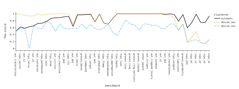
Figure 7: Comparison of AuToMATo and DBSCAN.

Table 3: Fowlkes-Mallows scores of AuToMATo vs. hierarchical clustering with average linkage

Dataset	automato_mean	linkage_average_max	linkage_average_min
sipu_r15_2	0.4867±0.0000	1.0000	0.3971
wut_trajectories_0	0.5038±0.0107	1.0000	0.3115
fcps_tetra_0	0.6261±0.0000	1.0000	0.0651
sipu_r15_1	0.5436±0.0000	0.8954	0.4435
sipu_d31_0	0.6001±0.0085	0.9322	0.1787
wut_x3_0	0.5153±0.0000	0.8389	0.3406
wut_x3_1	0.6546±0.0000	0.9747	0.2741
fcps_twodiamonds_0	0.7067±0.0000	0.9925	0.1287
sipu_a2_0	0.7555±0.0000	0.9432	0.1685
sipu_a1_0	0.7499±0.0000	0.9268	0.2229
sipu_a3_0	0.7434±0.0000	0.8825	0.1410
sipu_aggregation_0	0.8652±0.0000	0.9932	0.1788
sipu_pathbased_1	0.7322±0.0000	0.8564	0.2058
graves_dense_0	0.8377±0.1396	0.9604	0.6633
sipu_pathbased_0	0.6517±0.0000	0.7704	0.1848
wut_x2_0	0.5846±0.0000	0.7001	0.2782
wut_circles_0	0.8857±0.0000	1.0000	0.2369
wut_mk3_0	0.7720±0.0000	0.8771	0.0876
wut_mk2_0	0.6356±0.0000	0.7068	0.1421
sipu_r15_0	0.9258±0.0000	0.9900	0.2552
wut_x1_0	0.9483±0.1091	1.0000	0.3070
graves_zigzag_1	0.6720±0.0000	0.7202	0.4380
sipu_jain_0	0.7837±0.0000	0.7904	0.1736
wut_mk1_0	0.9866±0.0000	0.9933	0.2037
sipu_unbalance_0	0.9983±0.0009	0.9995	0.5339
fcps_hepta_0	1.0000±0.0000	1.0000	0.3727
sipu_flame_0	0.7320±0.0000	0.7320	0.0913
sipu_s1_0	0.9888±0.0000	0.9821	0.2581
sipu_compound_0	0.8616±0.0000	0.8431	0.2237
sipu_compound_4	0.9442±0.0000	0.9224	0.2011
sipu_compound_1	0.9786±0.0000	0.9546	0.1948
sipu_s2_0	0.9405±0.0000	0.9097	0.2581
wut_smile_1	0.9701±0.0000	0.8726	0.4041
fcps_atom_0	0.8694±0.0000	0.7491	0.2555
graves_parabolic_1	0.6916±0.0000	0.5708	0.2135
sipu_spiral_0	0.7028±0.0000	0.5756	0.1908
wut_mk4_0	0.9072±0.0234	0.7714	0.1982
wut_smile_0	0.9681±0.0000	0.8221	0.4303
wut_isolation_0	0.7256±0.0113	0.5773	0.1651
graves_line_0	1.0000±0.0000	0.8238	0.3047
fcps_wingnut_0	0.9805±0.0000	0.8016	0.1101
fcps_chainlink_0	0.8896±0.0000	0.7068	0.1456
fcps_target_0	0.9850±0.0000	0.7986	0.3285
fcps_lsun_0	1.0000±0.0000	0.7896	0.1735
graves_ring_0	1.0000±0.0000	0.7780	0.2638
graves_parabolic_0	0.9802±0.0000	0.7580	0.1598
graves_ring_outliers_0	1.0000±0.0000	0.7767	0.2801
other_square_0	1.0000±0.0000	0.7413	0.1746
wut_labirynth_0	0.7884±0.0000	0.5221	0.2306
wut_stripes_0	1.0000±0.0000	0.7070	0.1082
wut_twosplashes_0	1.0000±0.0000	0.7062	0.4837
wut_windows_0	1.0000±0.0000	0.6753	0.1194
wut_trapped_lovers_0	1.0000±0.0000	0.6632	0.1077
graves_zigzag_0	1.0000±0.0000	0.6616	0.3008

Table 3: Fowlkes-Mallows scores of AuToMATo vs. hierarchical clustering with average linkage

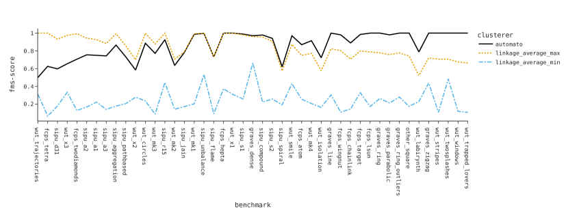
Figure 8: Comparison of AuToMATo and agglomerative clustering with average linkage.

Table 4: Fowlkes-Mallows scores of AuToMATo vs. HDBSCAN

Dataset	automato_mean	automato_std	hdbscan
wut_trajectories_0	0.5038±0.0107	0.0107	1.0000
wut_x3_0	0.5153±0.0000	0.0000	0.8959
wut_x2_0	0.5846±0.0000	0.0000	0.9344
sipu_spiral_0	0.7028±0.0000	0.0000	0.9815
sipu_flame_0	0.7320±0.0000	0.0000	1.0000
sipu_d31_0	0.6001±0.0085	0.0085	0.8234
sipu_jain_0	0.7837±0.0000	0.0000	0.9779
fcps_tetra_0	0.6261±0.0000	0.0000	0.8157
graves_dense_0	0.8377±0.1396	0.1396	0.9894
sipu_pathbased_1	0.7322±0.0000	0.0000	0.8634
fcps_atom_0	0.8694±0.0000	0.0000	1.0000
sipu_pathbased_0	0.6517±0.0000	0.0000	0.7815
fcps_chainlink_0	0.8896±0.0000	0.0000	1.0000
sipu_r15_0	0.9258±0.0000	0.0000	0.9932
sipu_a1_0	0.7499±0.0000	0.0000	0.8082
wut_x1_0	0.9483±0.1091	0.1091	1.0000
wut_x3_1	0.6546±0.0000	0.0000	0.6972
sipu_compound_1	0.9786±0.0000	0.0000	1.0000
sipu_compound_4	0.9442±0.0000	0.0000	0.9656
fcps_target_0	0.9850±0.0000	0.0000	1.0000
sipu_compound_0	0.8616±0.0000	0.0000	0.8751
sipu_unbalance_0	0.9983±0.0009	0.0009	1.0000
graves_zigzag_1	0.6720±0.0000	0.0000	0.6720
sipu_aggregation_0	0.8652±0.0000	0.0000	0.8652
wut_stripes_0	1.0000±0.0000	0.0000	1.0000
wut_trapped_lovers_0	1.0000±0.0000	0.0000	1.0000
wut_windows_0	1.0000±0.0000	0.0000	1.0000
fcps_hepta_0	1.0000±0.0000	0.0000	1.0000
fcps_lsun_0	1.0000±0.0000	0.0000	1.0000
graves_line_0	1.0000±0.0000	0.0000	1.0000
graves_ring_0	1.0000±0.0000	0.0000	1.0000
graves_ring_outliers_0	1.0000±0.0000	0.0000	1.0000
graves_zigzag_0	1.0000±0.0000	0.0000	1.0000
other_square_0	1.0000±0.0000	0.0000	1.0000
wut_mk3_0	0.7720±0.0000	0.0000	0.7719
wut_mk1_0	0.9866±0.0000	0.0000	0.9863
sipu_a2_0	0.7555±0.0000	0.0000	0.7515
sipu_a3_0	0.7434±0.0000	0.0000	0.7388
sipu_r15_2	0.4867±0.0000	0.0000	0.4671
sipu_r15_1	0.5436±0.0000	0.0000	0.5212
sipu_s1_0	0.9888±0.0000	0.0000	0.9117
wut_isolation_0	0.7256±0.0113	0.0113	0.6364
fcps_wingnut_0	0.9805±0.0000	0.0000	0.8715
sipu_s2_0	0.9405±0.0000	0.0000	0.7361
wut_mk4_0	0.9072±0.0234	0.0234	0.6459
wut_labirynth_0	0.7884±0.0000	0.0000	0.5116
graves_parabolic_1	0.6916±0.0000	0.0000	0.3616
fcps_twodiamonds_0	0.7067±0.0000	0.0000	0.2890
wut_mk2_0	0.6356±0.0000	0.0000	0.1575
wut_smile_0	0.9681±0.0000	0.0000	0.4000
wut_smile_1	0.9701±0.0000	0.0000	0.3714
graves_parabolic_0	0.9802±0.0000	0.0000	0.3526
wut_twosplashes_0	1.0000±0.0000	0.0000	0.3074
wut_circles_0	0.8857±0.0000	0.0000	0.1215

Table 4: Fowlkes-Mallows scores of AuToMATo vs. HDBSCAN

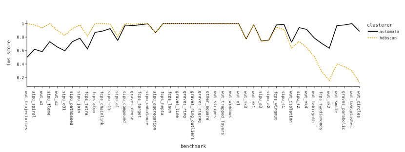
Figure 9: Comparison of AuToMATo and HDBSCAN.

Table 5: Fowlkes-Mallows scores of AuToMATo vs. hierarchical clustering with single linkage

Dataset	automato_mean	linkage_single_max	linkage_single_min
sipu_r15_2	0.4867±0.0000	1.0000	0.5607
wut_trajectories_0	0.5038±0.0107	1.0000	0.4999
sipu_r15_1	0.5436±0.0000	0.8954	0.5021
fcps_tetra_0	0.6261±0.0000	0.9296	0.0829
sipu_spiral_0	0.7028±0.0000	1.0000	0.5756
wut_isolation_0	0.7256±0.0113	1.0000	0.5773
wut_x3_0	0.5153±0.0000	0.7347	0.4951
sipu_jain_0	0.7837±0.0000	0.9510	0.7837
fcps_atom_0	0.8694±0.0000	1.0000	0.7067
wut_circles_0	0.8857±0.0000	1.0000	0.4998
fcps_chainlink_0	0.8896±0.0000	1.0000	0.7068
wut_mk4_0	0.9072±0.0234	1.0000	0.5770
sipu_compound_0	0.8616±0.0000	0.9454	0.4972
sipu_pathbased_0	0.6517±0.0000	0.7337	0.5769
sipu_pathbased_1	0.7322±0.0000	0.8091	0.5170
graves_dense_0	0.8377±0.1396	0.9096	0.6882
wut_mk2_0	0.6356±0.0000	0.7068	0.6007
graves_zigzag_1	0.6720±0.0000	0.7344	0.4446
wut_x2_0	0.5846±0.0000	0.6437	0.5105
wut_x1_0	0.9483±0.1091	0.9920	0.5846
wut_smile_1	0.9701±0.0000	1.0000	0.5825
fcps_target_0	0.9850±0.0000	1.0000	0.6963
wut_smile_0	0.9681±0.0000	0.9748	0.5471
sipu_unbalance_0	0.9983±0.0009	1.0000	0.5339
fcps_twodiamonds_0	0.7067±0.0000	0.7067	0.7067
wut_x3_1	0.6546±0.0000	0.6546	0.6140
sipu_aggregation_0	0.8652±0.0000	0.8652	0.4653
wut_stripes_0	1.0000±0.0000	1.0000	0.7070
wut_trapped_lovers_0	1.0000±0.0000	1.0000	0.6632
wut_windows_0	1.0000±0.0000	1.0000	0.6753
fcps_hepta_0	1.0000±0.0000	1.0000	0.3727
graves_line_0	1.0000±0.0000	1.0000	0.8238
graves_ring_0	1.0000±0.0000	1.0000	0.7068
graves_ring_outliers_0	1.0000±0.0000	1.0000	0.6863
graves_zigzag_0	1.0000±0.0000	1.0000	0.5381
sipu_flame_0	0.7320±0.0000	0.7320	0.4598
other_square_0	1.0000±0.0000	0.9990	0.7068
fcps_lsun_0	1.0000±0.0000	0.9983	0.6111
wut_twosplashes_0	1.0000±0.0000	0.9850	0.7062
sipu_compound_1	0.9786±0.0000	0.9180	0.5715
sipu_compound_4	0.9442±0.0000	0.8824	0.5523
wut_mk1_0	0.9866±0.0000	0.8866	0.5754
fcps_wingnut_0	0.9805±0.0000	0.8087	0.7068
graves_parabolic_1	0.6916±0.0000	0.5000	0.4979
wut_mk3_0	0.7720±0.0000	0.5764	0.5314
wut_labirynth_0	0.7884±0.0000	0.5221	0.5221
graves_parabolic_0	0.9802±0.0000	0.7068	0.7040
sipu_d31_0	0.6001±0.0085	0.1846	0.1787
sipu_a1_0	0.7499±0.0000	0.3269	0.2229
sipu_r15_0	0.9258±0.0000	0.4551	0.2552
sipu_a2_0	0.7555±0.0000	0.1685	0.1685
sipu_a3_0	0.7434±0.0000	0.1410	0.1410
sipu_s1_0	0.9888±0.0000	0.3695	0.2581
sipu_s2_0	0.9405±0.0000	0.2581	0.2579

Table 5: Fowlkes-Mallows scores of AuToMATo vs. hierarchical clustering with single linkage

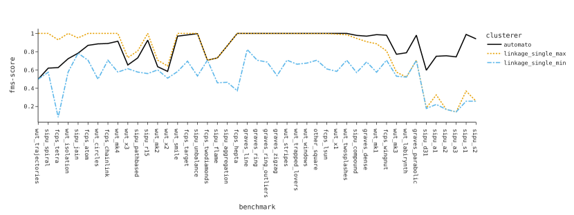
Figure 10: Comparison of AuToMATo and agglomerative clustering with single linkage.

Table 6: Fowlkes-Mallows scores of AuToMATo vs. TTK clustering algorithm

Dataset	automato_mean	automato_std	ttk
wut_trajectories_0	0.5038±0.0107	0.0107	0.8682
fcps_tetra_0	0.6261±0.0000	0.0000	0.9043
wut_x3_0	0.5153±0.0000	0.0000	0.7818
wut_isolation_0	0.7256±0.0113	0.0113	0.9416
sipu_a1_0	0.7499±0.0000	0.0000	0.9143
wut_x2_0	0.5846±0.0000	0.0000	0.7283
fcps_atom_0	0.8694±0.0000	0.0000	1.0000
sipu_flame_0	0.7320±0.0000	0.0000	0.8562
wut_mk3_0	0.7720±0.0000	0.0000	0.8852
sipu_aggregation_0	0.8652±0.0000	0.0000	0.9692
graves_zigzag_1	0.6720±0.0000	0.0000	0.7698
fcps_chainlink_0	0.8896±0.0000	0.0000	0.9464
sipu_jain_0	0.7837±0.0000	0.0000	0.8182
graves_dense_0	0.8377±0.1396	0.1396	0.8615
sipu_r15_0	0.9258±0.0000	0.0000	0.9374
wut_mk4_0	0.9072±0.0234	0.0234	0.9146
wut_labirynth_0	0.7884±0.0000	0.0000	0.7884
wut_smile_0	0.9681±0.0000	0.0000	0.9681
wut_stripes_0	1.0000±0.0000	0.0000	1.0000
wut_trapped_lovers_0	1.0000±0.0000	0.0000	1.0000
fcps_hepta_0	1.0000±0.0000	0.0000	1.0000
graves_ring_outliers_0	1.0000±0.0000	0.0000	1.0000
wut_smile_1	0.9701±0.0000	0.0000	0.9701
sipu_unbalance_0	0.9983±0.0009	0.0009	0.9951
sipu_s1_0	0.9888±0.0000	0.0000	0.9843
sipu_s2_0	0.9405±0.0000	0.0000	0.9311
wut_x3_1	0.6546±0.0000	0.0000	0.6312
sipu_d31_0	0.6001±0.0085	0.0085	0.5667
graves_parabolic_1	0.6916±0.0000	0.0000	0.6473
wut_x1_0	0.9483±0.1091	0.1091	0.8960
sipu_r15_2	0.4867±0.0000	0.0000	0.4322
sipu_pathbased_0	0.6517±0.0000	0.0000	0.5947
sipu_spiral_0	0.7028±0.0000	0.0000	0.6422
sipu_r15_1	0.5436±0.0000	0.0000	0.4827
sipu_pathbased_1	0.7322±0.0000	0.0000	0.6668
fcps_target_0	0.9850±0.0000	0.0000	0.9185
wut_twosplashes_0	1.0000±0.0000	0.0000	0.9140
wut_mk2_0	0.6356±0.0000	0.0000	0.5302
graves_parabolic_0	0.9802±0.0000	0.0000	0.8653
sipu_compound_4	0.9442±0.0000	0.0000	0.8145
fcps_wingnut_0	0.9805±0.0000	0.0000	0.8497
wut_circles_0	0.8857±0.0000	0.0000	0.7543
wut_mk1_0	0.9866±0.0000	0.0000	0.8148
fcps_twodiamonds_0	0.7067±0.0000	0.0000	0.5248
sipu_compound_0	0.8616±0.0000	0.0000	0.6728
sipu_compound_1	0.9786±0.0000	0.0000	0.7892
graves_line_0	1.0000±0.0000	0.0000	0.7917
fcps_lsun_0	1.0000±0.0000	0.0000	0.7897
other_square_0	1.0000±0.0000	0.0000	0.7774
graves_zigzag_0	1.0000±0.0000	0.0000	0.7686
graves_ring_0	1.0000±0.0000	0.0000	0.7278
sipu_a2_0	0.7555±0.0000	0.0000	0.4641
wut_windows_0	1.0000±0.0000	0.0000	0.5853
sipu_a3_0	0.7434±0.0000	0.0000	0.1882

Table 6: Fowlkes-Mallows scores of AuToMATo vs. TTK clustering algorithm

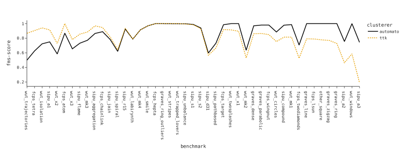
Figure 11: Comparison of AuToMATo and the TTK-algorithm.

Table 7: Fowlkes-Mallows scores of AuToMATo vs. hierarchical clustering with complete linkage

Dataset	automato_mean	linkage_complete_max	linkage_complete_min
sipu_r15_2	0.4867±0.0000	1.0000	0.2256
wut_trajectories_0	0.5038±0.0107	1.0000	0.1706
sipu_r15_1	0.5436±0.0000	0.8954	0.2516
wut_x3_1	0.6546±0.0000	0.9740	0.2004
fcps_tetra_0	0.6261±0.0000	0.9356	0.0651
wut_x3_0	0.5153±0.0000	0.7988	0.2477
sipu_d31_0	0.6001±0.0085	0.8733	0.2717
sipu_a3_0	0.7434±0.0000	0.8979	0.2294
wut_mk3_0	0.7720±0.0000	0.9207	0.0711
wut_x2_0	0.5846±0.0000	0.7298	0.1964
sipu_a2_0	0.7555±0.0000	0.8992	0.2642
sipu_jain_0	0.7837±0.0000	0.9116	0.1288
wut_circles_0	0.8857±0.0000	1.0000	0.1761
sipu_r15_0	0.9258±0.0000	0.9799	0.3372
sipu_a1_0	0.7499±0.0000	0.8040	0.3092
wut_x1_0	0.9483±0.1091	1.0000	0.2326
graves_zigzag_1	0.6720±0.0000	0.7119	0.3039
sipu_aggregation_0	0.8652±0.0000	0.8867	0.1243
sipu_unbalance_0	0.9983±0.0009	0.9988	0.5774
fcps_hepta_0	1.0000±0.0000	1.0000	0.4321
fcps_twodiamonds_0	0.7067±0.0000	0.7060	0.0916
sipu_flame_0	0.7320±0.0000	0.7276	0.0834
sipu_compound_0	0.8616±0.0000	0.8472	0.1567
sipu_compound_4	0.9442±0.0000	0.9224	0.1408
sipu_compound_1	0.9786±0.0000	0.9546	0.1366
sipu_s1_0	0.9888±0.0000	0.9516	0.3611
sipu_pathbased_0	0.6517±0.0000	0.6022	0.1384
sipu_pathbased_1	0.7322±0.0000	0.6709	0.1539
graves_parabolic_1	0.6916±0.0000	0.6168	0.1482
graves_dense_0	0.8377±0.1396	0.7584	0.3538
wut_mk1_0	0.9866±0.0000	0.8950	0.1591
wut_smile_1	0.9701±0.0000	0.8697	0.3562
graves_parabolic_0	0.9802±0.0000	0.8610	0.1088
wut_mk2_0	0.6356±0.0000	0.5032	0.1096
fcps_atom_0	0.8694±0.0000	0.7278	0.1364
wut_smile_0	0.9681±0.0000	0.8206	0.3793
sipu_s2_0	0.9405±0.0000	0.7642	0.3114
wut_mk4_0	0.9072±0.0234	0.7282	0.1297
fcps_wingnut_0	0.9805±0.0000	0.7883	0.0816
fcps_target_0	0.9850±0.0000	0.7881	0.1934
fcps_lsun_0	1.0000±0.0000	0.7668	0.1377
graves_ring_0	1.0000±0.0000	0.7589	0.1849
graves_ring_outliers_0	1.0000±0.0000	0.7528	0.1995
wut_labirynth_0	0.7884±0.0000	0.4893	0.1426
fcps_chainlink_0	0.8896±0.0000	0.5889	0.0919
sipu_spiral_0	0.7028±0.0000	0.3436	0.1362
wut_isolation_0	0.7256±0.0113	0.3397	0.1153
graves_line_0	1.0000±0.0000	0.5972	0.1909
other_square_0	1.0000±0.0000	0.5846	0.1142
graves_zigzag_0	1.0000±0.0000	0.5505	0.2042
wut_twosplashes_0	1.0000±0.0000	0.5310	0.2771
wut_stripes_0	1.0000±0.0000	0.5136	0.0706
wut_trapped_lovers_0	1.0000±0.0000	0.4790	0.0579
wut_windows_0	1.0000±0.0000	0.4349	0.0781

Table 7: Fowlkes-Mallows scores of AuToMATo vs. hierarchical clustering with complete linkage

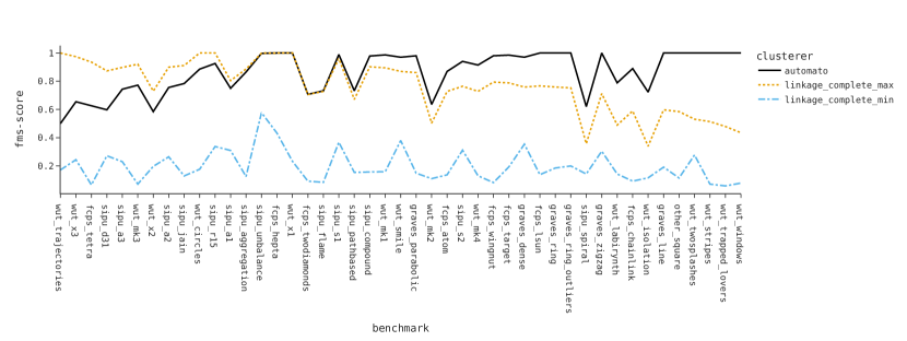
Figure 12: Comparison of AuToMATo and agglomerative clustering with complete linkage.

Table 8: Fowlkes-Mallows scores of AuToMATo vs. hierarchical clustering with Ward linkage

Dataset	automato_mean	linkage_ward_max	linkage_ward_min
wut_x3_0	0.5153±0.0000	0.8537	0.2187
sipu_d31_0	0.6001±0.0085	0.9223	0.2766
sipu_a3_0	0.7434±0.0000	0.9377	0.2892
sipu_a2_0	0.7555±0.0000	0.9360	0.2653
sipu_a1_0	0.7499±0.0000	0.9166	0.2464
wut_x2_0	0.5846±0.0000	0.7219	0.2076
sipu_r15_2	0.4867±0.0000	0.5893	0.1868
graves_zigzag_1	0.6720±0.0000	0.7358	0.2693
sipu_r15_0	0.9258±0.0000	0.9832	0.4072
sipu_r15_1	0.5436±0.0000	0.5993	0.2082
wut_x3_1	0.6546±0.0000	0.7090	0.1783
wut_x1_0	0.9483±0.1091	1.0000	0.2429
sipu_unbalance_0	0.9983±0.0009	1.0000	0.2099
fcps_hepta_0	1.0000±0.0000	1.0000	0.4314
sipu_s1_0	0.9888±0.0000	0.9844	0.2447
sipu_pathbased_0	0.6517±0.0000	0.6251	0.1370
sipu_s2_0	0.9405±0.0000	0.9085	0.2177
sipu_pathbased_1	0.7322±0.0000	0.6844	0.1523
fcps_tetra_0	0.6261±0.0000	0.5622	0.0651
graves_dense_0	0.8377±0.1396	0.7454	0.2684
wut_trajectories_0	0.5038±0.0107	0.3965	0.0980
fcps_atom_0	0.8694±0.0000	0.7272	0.1016
graves_parabolic_1	0.6916±0.0000	0.5260	0.1301
fcps_target_0	0.9850±0.0000	0.7759	0.1503
sipu_aggregation_0	0.8652±0.0000	0.6026	0.1214
sipu_flame_0	0.7320±0.0000	0.4555	0.0819
sipu_compound_0	0.8616±0.0000	0.5846	0.1524
wut_mk3_0	0.7720±0.0000	0.4911	0.0711
fcps_twodiamonds_0	0.7067±0.0000	0.3967	0.0861
sipu_jain_0	0.7837±0.0000	0.4668	0.1201
wut_mk1_0	0.9866±0.0000	0.6564	0.1473
fcps_lsun_0	1.0000±0.0000	0.6659	0.1270
sipu_compound_4	0.9442±0.0000	0.5793	0.1369
sipu_spiral_0	0.7028±0.0000	0.3123	0.1384
wut_labirynth_0	0.7884±0.0000	0.3749	0.0961
sipu_compound_1	0.9786±0.0000	0.5648	0.1329
wut_twosplashes_0	1.0000±0.0000	0.5817	0.2046
wut_smile_1	0.9701±0.0000	0.5246	0.2352
wut_smile_0	0.9681±0.0000	0.5179	0.2505
wut_mk2_0	0.6356±0.0000	0.1814	0.0997
graves_zigzag_0	1.0000±0.0000	0.5448	0.1809
wut_isolation_0	0.7256±0.0113	0.2309	0.0800
graves_line_0	1.0000±0.0000	0.5045	0.1667
wut_circles_0	0.8857±0.0000	0.3696	0.1323
fcps_chainlink_0	0.8896±0.0000	0.3407	0.0894
wut_mk4_0	0.9072±0.0234	0.3557	0.1079
graves_parabolic_0	0.9802±0.0000	0.4184	0.0935
graves_ring_0	1.0000±0.0000	0.4135	0.1427
graves_ring_outliers_0	1.0000±0.0000	0.4082	0.1515
fcps_wingnut_0	0.9805±0.0000	0.3176	0.0727
other_square_0	1.0000±0.0000	0.3347	0.1007
wut_windows_0	1.0000±0.0000	0.2847	0.0663
wut_trapped_lovers_0	1.0000±0.0000	0.2552	0.0471
wut_stripes_0	1.0000±0.0000	0.1922	0.0552

Table 8: Fowlkes-Mallows scores of AuToMATo vs. hierarchical clustering with Ward linkage

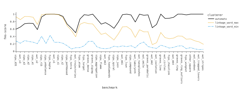
Figure 13: Comparison of AuToMATo and agglomerative clustering with Ward linkage.

Table 9: Fowlkes-Mallows scores of AuToMATo vs. FINCH

Dataset	automato_mean	automato_std	finch
wut_x3_0	0.5153±0.0000	0.0000	0.7970
sipu_d31_0	0.6001±0.0085	0.0085	0.8657
sipu_a3_0	0.7434±0.0000	0.0000	0.8306
wut_x2_0	0.5846±0.0000	0.0000	0.6671
wut_mk3_0	0.7720±0.0000	0.0000	0.8503
sipu_a2_0	0.7555±0.0000	0.0000	0.7635
wut_x3_1	0.6546±0.0000	0.0000	0.6619
sipu_unbalance_0	0.9983±0.0009	0.0009	0.9998
sipu_r15_0	0.9258±0.0000	0.0000	0.9083
wut_mk1_0	0.9866±0.0000	0.0000	0.9655
sipu_a1_0	0.7499±0.0000	0.0000	0.7124
sipu_r15_2	0.4867±0.0000	0.0000	0.4156
graves_zigzag_1	0.6720±0.0000	0.0000	0.5965
graves_dense_0	0.8377±0.1396	0.1396	0.7615
sipu_r15_1	0.5436±0.0000	0.0000	0.4641
sipu_s1_0	0.9888±0.0000	0.0000	0.8728
fcps_hepta_0	1.0000±0.0000	0.0000	0.8794
fcps_atom_0	0.8694±0.0000	0.0000	0.7319
fcps_tetra_0	0.6261±0.0000	0.0000	0.4680
wut_x1_0	0.9483±0.1091	0.1091	0.7607
sipu_s2_0	0.9405±0.0000	0.0000	0.7282
graves_parabolic_1	0.6916±0.0000	0.0000	0.4446
sipu_flame_0	0.7320±0.0000	0.0000	0.4717
sipu_pathbased_0	0.6517±0.0000	0.0000	0.3440
sipu_compound_0	0.8616±0.0000	0.0000	0.5365
sipu_pathbased_1	0.7322±0.0000	0.0000	0.3828
wut_trajectories_0	0.5038±0.0107	0.0107	0.1506
fcps_lsun_0	1.0000±0.0000	0.0000	0.6206
sipu_compound_4	0.9442±0.0000	0.0000	0.5536
sipu_jain_0	0.7837±0.0000	0.0000	0.3828
sipu_compound_1	0.9786±0.0000	0.0000	0.5397
sipu_spiral_0	0.7028±0.0000	0.0000	0.2477
wut_mk4_0	0.9072±0.0234	0.0234	0.4331
wut_mk2_0	0.6356±0.0000	0.0000	0.1478
sipu_aggregation_0	0.8652±0.0000	0.0000	0.3679
fcps_twodiamonds_0	0.7067±0.0000	0.0000	0.1837
wut_smile_0	0.9681±0.0000	0.0000	0.4452
wut_smile_1	0.9701±0.0000	0.0000	0.4181
fcps_target_0	0.9850±0.0000	0.0000	0.4297
wut_labirynth_0	0.7884±0.0000	0.0000	0.2209
wut_isolation_0	0.7256±0.0113	0.0113	0.1433
wut_twosplashes_0	1.0000±0.0000	0.0000	0.4162
graves_zigzag_0	1.0000±0.0000	0.0000	0.4094
graves_parabolic_0	0.9802±0.0000	0.0000	0.3343
graves_line_0	1.0000±0.0000	0.0000	0.3379
fcps_chainlink_0	0.8896±0.0000	0.0000	0.2224
fcps_wingnut_0	0.9805±0.0000	0.0000	0.3094
graves_ring_0	1.0000±0.0000	0.0000	0.2770
wut_trapped_lovers_0	1.0000±0.0000	0.0000	0.2767
other_square_0	1.0000±0.0000	0.0000	0.2393
graves_ring_outliers_0	1.0000±0.0000	0.0000	0.2248
wut_circles_0	0.8857±0.0000	0.0000	0.0975
wut_windows_0	1.0000±0.0000	0.0000	0.1166
wut_stripes_0	1.0000±0.0000	0.0000	0.0868

Table 9: Fowlkes-Mallows scores of AuToMATo vs. FINCH

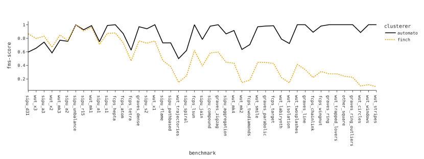
Figure 14: Comparison of AuToMATo and FINCH.

References

- [And73] Michael R. Anderberg. Index. In Cluster Analysis for Applications, Probability and Mathematical Statistics: A Series of Monographs and Textbooks, pages 355–359. Academic Press, 1973.
- [BCCS+11] Gérard Biau, Frédéric Chazal, David Cohen-Steiner, Luc Devroye, and Carlos Rodríguez. A weighted k-nearest neighbor density estimate for geometric inference. Electronic Journal of Statistics, 5(none):204 – 237, 2011.
- [Boc07] Hans-Hermann Bock. Clustering methods: a history of k-means algorithms. Selected contributions in data analysis and classification, pages 161–172, 2007.
- [BTO24] Alexandre Bois, Brian Tervil, and Laurent Oudre. Persistence-based clustering with outlier-removing filtration. Frontiers in Applied Mathematics and Statistics, 10, 2024.
- [Car14] Gunnar Carlsson. Topological pattern recognition for point cloud data. Acta Numerica, 23:289–368, 2014.
- [CCSG+09] Frédéric Chazal, David Cohen-Steiner, Leonidas J. Guibas, Facundo Mémoli, and Steve Y. Oudot. Gromov-hausdorff stable signatures for shapes using persistence. Computer Graphics Forum, 28(5):1393–1403, 2009.
- [CdSMS16] F. Chazal, V. de Silva, Glisse M., and Oudot S. The Structure and Stability of Persistence Modules. Springer, 2016.
- [CdSO14] F. Chazal, V. de Silva, and S. Oudot. Persistence stability for geometric complexes. Geometriae Dedicata, 173:193–214, 2014. https://doi.org/10.1007/s10711-013-9937-z.
- [CFL+17] Frédéric Chazal, Brittany Fasy, Fabrizio Lecci, Bertrand Michel, Alessandro Rinaldo, and Larry A. Wasserman. Robust topological inference: Distance to a measure and kernel distance. J. Mach. Learn. Res., 18:159:1–159:40, 2017.
- [CGOS13] Frédéric Chazal, Leonidas J Guibas, Steve Y Oudot, and Primoz Skraba. Persistence-based clustering in riemannian manifolds. Journal of the ACM (JACM), 60(6):1–38, 2013.
- [CMO18] Mathieu Carrière, Bertrand Michel, and Steve Oudot. Statistical analysis and parameter selection for mapper. Journal of Machine Learning Research, 19(12):1–39, 2018.
- [CMS13] Ricardo JGB Campello, Davoud Moulavi, and Jörg Sander. Density-based clustering based on hierarchical density estimates. In Pacific-Asia conference on knowledge discovery and data mining, pages 160–172. Springer, 2013.
- [COGDS16] Frédéric Chazal, Steve Y. Oudot, Marc Glisse, and Vin De Silva. The Structure and Stability of Persistence Modules. SpringerBriefs in Mathematics. Springer Verlag, 2016.
- [CSEH07] David Cohen-Steiner, Herbert Edelsbrunner, and John Harer. Stability of persistence diagrams. Discrete & Computational Geometry, 37(1):103–120, Jan 2007.
- [CSTL21] Ryan Cotsakis, Jim Shaw, Julien Tierny, and Joshua A. Levine. Implementing persistence-based clustering of point clouds in the topology toolkit. In Ingrid Hotz, Talha Bin Masood, Filip Sadlo, and Julien Tierny, editors, Topological Methods in Data Analysis and Visualization VI, pages 343–357, Cham, 2021. Springer International Publishing.
- [CZW21] Nithin Chalapathi, Youjia Zhou, and Bei Wang. Adaptive covers for mapper graphs using information criteria. In 2021 IEEE International Conference on Big Data (Big Data), pages 3789–3800, 2021.
- [DHS00] Richard O. Duda, Peter E. Hart, and David G. Stork. Pattern Classification (2nd Edition). Wiley-Interscience, USA, 2000.
- [EH10] H. Edelsbrunner and J. Harer. Computational Topology: An Introduction. Applied Mathematics. American Mathematical Society, 2010.
- [EIK01] A. Efrat, A. Itai, and M. J. Katz. Geometry helps in bottleneck matching and related problems. Algorithmica, 31(1):1–28, Sep 2001.
- [EKSX96] Martin Ester, Hans-Peter Kriegel, Jörg Sander, and Xiaowei Xu. A density-based algorithm for discovering clusters in large spatial databases with noise. In Proceedings of the Second International Conference on Knowledge Discovery and Data Mining, KDD’96, page 226–231. AAAI Press, 1996.
- [ELZ02] Edelsbrunner, Letscher, and Zomorodian. Topological persistence and simplification. Discrete & Computational Geometry, 28(4):511–533, Nov 2002.
- [FM83] Edward B Fowlkes and Colin L Mallows. A method for comparing two hierarchical clusterings. Journal of the American statistical association, 78(383):553–569, 1983.
- [Gli23] Marc Glisse. persistence-based clustering. In GUDHI User and Reference Manual. GUDHI Editorial Board, 3.9.0 edition, 2023. Available under MIT license.
- [Hat02] Allen Hatcher. Algebraic topology. Cambridge University Press, 2002.
- [Loa24] Catherine Loader. locfit: Local Regression, Likelihood and Density Estimation, 2024. R package version 1.5-9.9.
- [MT13] Krishna K Mohbey and GS Thakur. An experimental survey on single linkage clustering. International Journal of Computer Applications, 76(17):6–11, 2013.
- [Ran71] William M. Rand. Objective criteria for the evaluation of clustering methods. Journal of the American Statistical Association, 66(336):846–850, 1971.
- [RF16] Mohammad Rezaei and Pasi Fränti. Set matching measures for external cluster validity. IEEE Transactions on Knowledge and Data Engineering, 28(8):2173–2186, 2016.
- [RHW23] P. Rosen, M. Hajij, and B. Wang. Homology-preserving multi-scale graph skeletonization using mapper on graphs. In 2023 Topological Data Analysis and Visualization (TopoInVis), pages 10–20, Los Alamitos, CA, USA, oct 2023. IEEE Computer Society.
- [RVBV16] Simone Romano, Nguyen Xuan Vinh, James Bailey, and Karin Verspoor. Adjusting for chance clustering comparison measures. Journal of Machine Learning Research, 17(134):1–32, 2016.
- [SB+19] Shweta Sharma, Neha Batra, et al. Comparative study of single linkage, complete linkage, and ward method of agglomerative clustering. In 2019 international conference on machine learning, big data, cloud and parallel computing (COMITCon), pages 568–573. IEEE, 2019.
- [SMC+07] Gurjeet Singh, Facundo Mémoli, Gunnar E Carlsson, et al. Topological methods for the analysis of high dimensional data sets and 3d object recognition. PBG@ Eurographics, 2:091–100, 2007.
- [SSS19] M. Saquib Sarfraz, Vivek Sharma, and Rainer Stiefelhagen. Efficient parameter-free clustering using first neighbor relations. In Proceedings of the IEEE Conference on Computer Vision and Pattern Recognition (CVPR), pages 8934–8943, 2019.
- [TFL+18] Julien Tierny, Guillaume Favelier, Joshua A. Levine, Charles Gueunet, and Michael Michaux. The topology toolkit. IEEE Transactions on Visualization and Computer Graphics, 24(1):832–842, January 2018. Funding Information: This work is partially supported by the Bpifrance grant “AVIDO” (Programme d’Investissements d’Avenir FSN2, reference P112017-2661376/DOS0021427) and by the National Science Foundation IIS-1654221. We would like to thank the reviewers for their thoughtful remarks and suggestions. We would also like to thank Attila Gyulassy, Julien Jomier and Joachim Pouderoux for insightful discussions and Will Schroeder, who encouraged us to write this manuscript. Publisher Copyright: © 1995-2012 IEEE.
- [TLT+20] Guillaume Tauzin, Umberto Lupo, Lewis Tunstall, Julian Burella Pérez, Matteo Caorsi, Anibal Medina-Mardones, Alberto Dassatti, and Kathryn Hess. giotto-tda: A topological data analysis toolkit for machine learning and data exploration, 2020.
- [VEB10] Nguyen Xuan Vinh, Julien Epps, and James Bailey. Information theoretic measures for clusterings comparison: Variants, properties, normalization and correction for chance. J. Mach. Learn. Res., 11:2837–2854, dec 2010.
- [ZC05] Afra Zomorodian and Gunnar Carlsson. Computing persistent homology. Discrete & Computational Geometry, 33(2):249–274, Feb 2005.